Manipulating Deformable Objects by Interleaving Prediction, Planning, and Control
Abstract
We present a framework for deformable object manipulation that interleaves planning and control, enabling complex manipulation tasks without relying on high-fidelity modeling or simulation. The key question we address is when should we use planning and when should we use control to achieve the task? Planners are designed to find paths through complex configuration spaces, but for highly underactuated systems, such as deformable objects, achieving a specific configuration is very difficult even with high-fidelity models. Conversely, controllers can be designed to achieve specific configurations, but they can be trapped in undesirable local minima due to obstacles. Our approach consists of three components: (1) A global motion planner to generate gross motion of the deformable object; (2) A local controller for refinement of the configuration of the deformable object; and (3) A novel deadlock prediction algorithm to determine when to use planning versus control. By separating planning from control we are able to use different representations of the deformable object, reducing overall complexity and enabling efficient computation of motion. We provide a detailed proof of probabilistic completeness for our planner, which is valid despite the fact that our system is underactuated and we do not have a steering function. We then demonstrate that our framework is able to successfully perform several manipulation tasks with rope and cloth in simulation which cannot be performed using either our controller or planner alone. These experiments suggest that our planner can generate paths efficiently, taking under a second on average to find a feasible path in three out of four scenarios. We also show that our framework is effective on a 16 DoF physical robot, where reachability and dual-arm constraints make the planning more difficult.
1 Introduction
Examples of deformable object manipulation range from domestic tasks like folding clothes to time and safety critical tasks such as robotic surgery. One of the challenges in planning for deformable object manipulation is the high number of degrees of freedom involved; even approximating the configuration of a piece of cloth in 3D with a 4 4 grid results in a 48 degree of freedom configuration space. In addition, the dynamics of the deformable object are difficult to model (Essahbi et al. 2012); even with high-fidelity modeling and simulation, planning for an individual task can take hours (Bai et al. 2016). Local controllers on the other hand are able to very efficiently generate motion, however, they are only able to successfully complete a task when the initial configuration is in the “attraction basin” of the goal (Berenson 2013; McConachie and Berenson 2018).


The central question we address in this work is how can we combine the strengths of global planning with the strengths of local control while mitigating the weakness of each? We propose a framework for interleaving planning and control which uses global planning to generate gross motion of the deformable object, and a local controller to refine the configuration of the deformable object within the local neighborhood. By separating planning from control we are able to use different representations of the deformable object, each suited to efficient computation for their respective roles. In order to determine when to use each component, we introduce a novel deadlock prediction algorithm that is inspired by topologically-based motion planning methods (Bhattacharya et al. 2012; Jaillet and Siméon 2008). By answering the question “Will the local controller get stuck?” we can predict if the local controller will be unable to achieve the task from the current configuration. If we predict that the controller will get stuck we can then invoke the global planner, moving the deformable object into a new neighbourhood from which the local controller may be able to succeed. The key to our efficient prediction is forward-propagating only the stretching constraint, assuming the object will otherwise comply to contact.
We seek to solve problems for one-dimensional and two-dimensional deformable objects (i.e. rope and cloth) where we need to arrange the object in a particular way (e.g. covering a table with a tablecloth) but where there is also complex environment geometry preventing us from directly completing the task. While we cannot claim to solve all problems in this class (in particular in environments where the deformable object can be snagged), we can still solve practical problems where the path of the deformable object is obstructed by obstacles. In this work we restrict our focus to controllers of the form described in Sec. 4.1, and tasks suited to these controllers. Examples of these types of tasks are shown in Fig. 1. In our experiments we show that this iterative method of interleaving planning and control is able to successfully perform several interesting tasks where our planner or controller alone are unable to succeed.
Our contributions are: (1) A novel deadlock prediction algorithm to determine when a global planner is needed; (2) An efficient and probabistically-complete global planner for rope and cloth manipulation tasks; and (3) A framework to combine local control and global motion planning to leverage the strengths of each while mitigating their weaknesses. We present experiments in both a simulated environment and on a physical robot (Fig. 1). Our results suggest that our planner can efficiently find paths, taking under a second on average to generate a feasible path in three out of four simulated scenarios. The physical experiment shows that our framework is able to effectively perform tasks in the real world, where reachability and dual-arm constraints make the planning more difficult.
A preliminary version of this work was presented in McConachie et al. 2017. This paper extends this work by adding an additional experiment on a physical robotic system as well as a proof of the probabilistic completeness of our planning method. We have also improved planning times with an improved goal bias method. We also include additional related work and an expanded discussion.
2 Related Work
Robotic manipulation of deformable objects has been studied in many contexts ranging from surgery to industrial manipulation (see Khalil and Payeur 2010 and Sanchez et al. 2018 for extensive surveys). Below we discuss the most relevant methods to the work presented here, starting with methods of simulating and planning for deformable objects. We then discuss visual servoing and learning-based methods for similar tasks. In addition to previous work in deformable object manipulation, we also discuss related work in planning/control for robot arms and ways to consider topology in planning, which we draw from for our framework. We end with a discussion of probabilistic completeness and describe why previous methods to show this property do not apply, motivating our proof method.
Much work in deformable object manipulation relies on simulating an accurate model of the object being manipulated. Motivated by applications in computer graphics and surgical training, many methods have been developed for simulating string-like objects (Bergou et al. 2008; Rungjiratananon et al. 2011) and cloth-like objects (Baraff and Witkin 1998; Goldenthal et al. 2007). The most common simulation methods use Mass-Spring models (Gibson and Mirtich 1997; Essahbi et al. 2012), which are generally not accurate for large deformations (Maris et al. 2010), and Finite-Element (FEM) models (Müller et al. 2002; Irving et al. 2004; Kaufmann et al. 2008). FEM-based methods are widely used and physically well-founded, but they can be unstable when subject to contact constraints, which are especially important in this work. They also require significant tuning and are very sensitive to the discretization of the object. Furthermore, such models require knowledge of the physical properties of the object, such as it’s Young’s modulus and friction parameters, which we do not assume are known.
Motion planning for manipulation of deformable objects is an active area of research (Jiménez 2012). Saha et al. 2008 present a Probabilistic Roadmap (PRM) (Kavraki et al. 1996) that plans for knot-tying tasks with rope. Rodriguez and Amato 2006 study motion planning in fully deformable simulation environments. Their method, based on Rapidly-exploring Random Trees (RRTs) (LaValle 2006), applies forces directly to an object to move it through narrow spaces while using the simulator to compute the resulting deformations. Frank et al. 2011 presented a method that pre-computes deformation simulations in a given environment to enable fast multi-query planning. Other sampling-based approaches have also been proposed (Anshelevich et al. 2000; Burchan Bayazit et al. 2002; Gayle et al. 2005; Lamiraux and Kavraki 2001; Moll and Kavraki 2006; Roussel et al. 2015). However, all the above methods either disallow contact with the environment or rely on potentially time-consuming physical simulation of the deformable object, which is often very sensitive to physical and computational parameters that may be difficult to determine. In contrast our method uses simplified models for control and motion planning with far lower computational cost. In addition, the use of a local controller is not considered in the above methods, instead relying on a global planner (and thus implicitly the accuracy of the simulator) to generate a path that completes the entire task.
Model-based visual servoing approaches bypass planning entirely, and instead use a local controller to determine how to move the robot end-effector for a given task (Hirai and Wada 2000; Smolen and Patriciu 2009; Wada et al. 2001). Our recent work (Berenson 2013; McConachie and Berenson 2018) as well as Navarro-Alarcon et al. 2014; Navarro-Alarcon et al. 2016; Navarro-Alarcon and Liu 2018 bypass the need for an explicit deformable object model, instead using approximations of the Jacobian to drive the deformable object to the attractor of the starting state. More recent work by Hu et al. 2018 has enabled the use of Gaussian process regression while controlling a deformable object. Rather than using only a planner or only a controller, our framework uses both components, each when appropriate.
Approaches based on learning from demonstration avoid planning and deformable object modelling challenges entirely by using offline demonstrations to teach the robot specific manipulation tasks (Huang et al. 2015; Schulman et al. 2016); however, when a new task is attempted a new training set needs to be generated. In our application we are interested in a way to manipulate a deformable object without a high-fidelity model or training set available a priori. For instance, imagine a robot encountering a new piece of clothing for a new task. While it may have models for previously-seen clothes or training sets for previous tasks, there is no guarantee that those models or training sets are appropriate for the new task.
Park et al. 2014 considered interleaving planning and control for arm reaching tasks in rigid unknown environments. In their method, they assume an initially unknown environment in which they plan a path to a specific end-effector position. This path is then followed by a local controller until the task is complete, or the local controller gets stuck. If the local controller gets stuck, then a new path is planned and the cycle repeats. In contrast, our controller is performing the task directly rather than following a planned reference trajectory, incorporating deadlock prediction into the execution loop, while our global planner is planning for both the robot motion as well as the deformable object stretching constraint.
Our planning method has some similarity to topological (Bhattacharya et al. 2012; Jaillet and Siméon 2008) and tethered robot (Brass et al. 2015; Kim and Likhachev 2015) planning techniques; these methods use the topological structure of the space to define homotopy classes, either as a direct planning goal, or as a way to help inform planning in the case of tethered robots. Planning for some deformable objects, in particular rope or string, can be viewed as an extension of the tethered robot case where the base of the tether can move. This extension, however, requires a very different approach to homotopy than is commonly used, particularly when working in three-dimensional space instead of a planar environment. In our work we use visiblity deformations from Jaillet and Siméon 2008 as a way to encode homotopy-like classes of configurations.
Previous approaches to proving probabilistic completeness for efficient planning of underactuated systems rely on the existence of a steering function to move the system from one region of the state space to another, or choosing controls at random (LaValle and Kuffner 2001; Karaman and Frazzoli 2013; Kunz and Stilman 2015; Li et al. 2016). For deformable objects, a computationally-efficient steering function is not available, and using random controls can lead to prohibitively long planning times. Roussel et al. 2015 bypass this challenge by analyzing completeness in the submanifold of quasi-static contact-free configurations of a extensible elastic rods. In contrast, we show that our method is probabilistically complete even when contact between the deformable object and obstacles is considered along the path. Note that it is especially important to allow contact at the goal configuration of the object to achieve coverage tasks. Li et al. 2016 present an efficient asymptotically-optimal planner which does not need a steering function, however, they do rely on the existence of a contact free trajectory where every point in the trajectory is in the interior of the valid configuration space. Our proof of probabilistic completeness is based on Li et al. 2016, but we allow for the deformable object to be in contact with obstacles along a given trajectory.
3 Problem Statement
Define the robot configuration space to be . We assume that the robot configuration can be measured exactly. Denote an individual robot configuration as . This set can be partitioned into a valid and invalid set. The valid set is referred to as , and is the set of configurations where the robot is not in collision with the static geometry of the world. The invalid set is referred to as .
We assume that our model of the robot is purely kinematic, with no higher order dynamics. We assume that the robot has two end-effectors that are rigidly attached to the object. The configuration of a deformable object is a set of points. We assume that we have a method of sensing . The rest of the environment is denoted and is assumed to be both static, and known exactly. We assume that the robot moves slowly enough that we can treat the combined robot and deformable object as quasi-static. Let the function map the system configuration and robot movement to the corresponding deformable object movement . We assume that the deformable object will be damaged if it is stretched beyond a factor from the relaxed state. Let be the symmetric matrix of pairwise distances between all points of in its relaxed state. We assume that there are no other deformable object properties (such as bending energy) that are relevant to the task.
We define a task based on a set of target points , a function , which measures the alignment error between and , and a termination function which indicates if the task is finished. Let a robot controller be a function 11 1 A specific controller may have additional parameters (such as gains in a PID controller), but we do not include such parameters here to keep in a more general form. which maps the system state and alignment targets to a desired robot motion . In this work we restrict our discussion to tasks and controllers of the form introduced in our previous work (Berenson 2013; McConachie and Berenson 2018); these controllers are local, i.e. at each time they choose an incremental movement which reduces the alignment error as much as possible at time .
The problem we address in this work is how to find a sequence of robot commands such that each motion is feasible, i.e. it should not bring the grippers into collision with obstacles, should not cause the object to stretch excessively, and should not exceed the robot’s maximum velocity . Let these feasibility constraints be represented by . Then the problem we seek to solve is:
| (1) | ||||||
where is the configuration of the deformable object after executing .
Solving this problem directly is impractical in the general case for two major reasons. First, modeling a deformable object accurately is very difficult in the general case, especially if it contacts other objects or itself. Second, even given a perfect model, computing precise motion of the deformable object requires physical simulation, which can be very time consuming inside a planner/controller where many potential movements need to be evaluated. We seek a method which does not rely on high-fidelity modelling and simulation; instead we present a framework combining both global planning and local control to leverage the strengths of each in order to efficiently perform the task.
4 Interleaving Planning and Control
Global planners are effective at finding paths through complex configuration spaces, but for highly underactuated systems such as deformable objects achieving a specific configuration is very difficult even with high-fidelity models; this means that we cannot rely on them to complete a task independent of a local controller. In order for the local controller to complete the task, the system must be in the correct basin of attraction. From this point of view it is not the planner’s responsibility to complete a task but rather to move the system into the right basin for the local controller to finish the task. By explicitly separating planning from control we can use different representations of the deformable object for each component; this allows us to use a highly-simplified model of the deformable object for global planning to generate gross motion of the deformable object, while using an independent local approximation for the controller. The key question then is when should we use global planning versus local control?
Our framework can be broken down into three major components: (1) A global motion planner to generate gross motion of the deformable object; (2) A local controller for refinement of the configuration of the deformable object; and (3) A novel deadlock prediction algorithm to determine when to use planning versus control. Fig. 2 shows how these components are connected, switching between a local controller loop and planned path execution loop as needed. In the following sections we describe each component in turn, starting with the local controller.
4.1 Local Control
The role of the local controller is not to perform the whole task, but rather to refine the configuration of the deformable object locally. For our local controller we use a controller of the form introduced in Berenson 2013 and McConachie and Berenson 2018. These controllers locally minimize error while avoiding robot collision and excessive stretching of the deformable object.
An outline of how these controllers function is shown in Alg. 1; first, for every target point we define a workspace navigation function pointing towards using Dijkstra’s algorithm. This gives us the shortest collision-free path between any point in the workspace and the target point, as well as the distance travelled along that path. These navigation functions are used to define the best direction to move the deformable object and the relative importance of each part of the motion in order to locally reduce error as much as possible at each timestep (Lines 1 and 2). These error reduction terms are then combined using relative importance weight with stretching avoidance terms to define the desired manipulation direction and importance weights at each timestep (Lines 3 and 4). If these terms conflict, then stretching correction takes precedence. We then find the best robot motion to achieve the desired deformable object motion, while preventing collision between the robot and obstacles (Line 5).
Given the current system state FindBestRobotMotion is solving the following problem:
| (2) | ||||||
How Eq. (2) is solved depends on the particular robot; details for each function in Alg. 1 are in Appendix A.
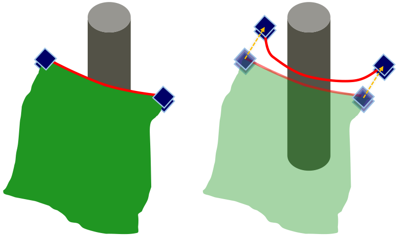
An important limitation of this approach is that the individual navigation functions are defined and applied independently of each other; this means that the navigation functions that are combined to define the direction to move the deformable object can cause the controller to move the end effectors on opposite sides of an obstacle, leading to poor local minima, i.e. becoming stuck. Figure 3 shows our motivating example of this type of situation. Other examples of this kind of situation are shown in Section 7. In addition, while this local controller prevents collision between the robot and obstacles, it does not explicitly have any ability to go around obstacles.
In order to address these limitations we introduce a novel deadlock prediction algorithm to detect when the system is in a state that will lead to deadlock (i.e. becoming stuck) if we continue to use the local controller.
4.2 Predicting Deadlock
Predicting deadlock is important for two reasons; first we do not want to waste time executing motions that will not achieve the task. Second, we want to avoid the computational expense of planning our way out of a cul-de-sac after reaching a stuck state. By predicting deadlock before it happens we address both of these concerns. The key idea is to detect situations similar to Figure 3 where the local controller will wrap the deformable object around an obstacle without completing the task. We also need to detect situations where no progress can be made due to an obstacle directly in the path of the desired motion of the robot.
Let be the true motion of the robot when is executed for unit time; in this section we will be predicting the future state of the system, thus it is not sufficient to consider only , we must also consider . Modelling inaccuracies as well as the deformable object being in contact can lead to meaningful differences between and . Specifically, when a deformable object is in contact with the environment, tracking perfectly may lead to a constraint violation (i.e. overstretch or tearing of the deformable object).
We consider a controller to be deadlocked if the commanded motion produces (nearly) no actual motion, and the task termination condition is not met:
| (3) |
In general we cannot predict if the system will get stuck in the limit; to do so would require a very accurate simulation of the deformable object. Instead we predict if the system will get stuck within a prediction horizon timesteps. We divide our deadlock prediction algorithm into three parts and discuss each in turn: 1) estimating gross motion; 2) predicting overstretch; and 3) progress detection.
4.2.1 Estimating Gross Motion:
The idea central to our prediction (Alg. 2) is that while we may not be able to determine precisely how a given controller will steer the system, we can capture the gross motion of the system and estimate if the controller will be deadlocked. We split the prediction into two parts; first we assume that controller is able to manipulate the deformable object with a reasonable degree of accuracy within a local neighborhood of the current state. This allows us to approximate the motion of the deformable object by following the task-defined navigation functions for each . Examples of this approximation are shown in Figure 4.
Next we use a simplified version of LocalController() which omits the stretching avoidance terms (Alg. 1 lines 3 and 4) to predict the commands sent to the robot. These terms are omitted as they can be sensitive to the exact configuration of the deformable object, which is not considered in this approximation. If we are executing a path then we can use the planned path directly to predict overstretch.
| do |
| Path | then |
| PredictOverstretch or | |
| NoProgressConfigHistory, ErrorHistory | then |
4.2.2 Predicting Overstretch:
Next we introduce the notion of a virtual elastic band between the robot’s end-effectors. This elastic band represents the shortest path through the deformable object between the end-effectors. The band approximates the constraint imposed by the deformable object on the motion of the robot; if the end-effectors move too far apart, then the elastic band will be too long, and thus the deformable object is stretched beyond a task-specified maximum stretching factor . Similarly, if the elastic band gets caught on an obstacle and becomes too long, then the deformable object is also overstretched. By considering only the geodesic between the end-effectors, we are assuming that the rest of deformable object will comply to the environment, and does not need to be considered when predicting overstretch. The elastic band representation allows us to use a fast prediction method, but does not account for the part of the material that is slack. We discuss this trade-off further in Section 9. This virtual elastic band is based on Quinlan’s path deformation algorithm Quinlan 1994 and is used both in deadlock prediction as well as global planning (Sec. 4.3 and Sec. 5)
Denote the configuration of an elastic band at time as a sequence of points . The number of points used to represent an elastic band can change over time, but for any given environment and deformable object there is an upper limit on the number of points used. Define to be the straight line interpolation of all points in . Define the length of a band to be the length of this straight line interpolation. At each timestep the elastic band is initialized with the shortest path between the end effectors through the deformable object, and then “pulled” tight using the internal contraction force described in Quinlan 1994 §5, and a hard constraint for collision avoidance. The endpoints of the band track the predicted translation of the end effectors (Alg. 3). This band represents the constraint that must be satisfied for the object not to tear. By considering only this constraint on the object in prediction, we are implicitly relying on the object to comply to contact as it is moved by the robot. We discuss the limitations of this assumption in the discussion (Sec. 9).
Let be the length of the path defined by the virtual elastic band at timestep in the future, and be the longest allowable band length. To use this length sequence to predict if the controller will overstretch the deformable object, we perform three filtering steps: an annealing low-pass filter, a filter to eliminate cases where the band is in freespace, and the detector itself which predicts overstretch. We use a low-pass annealing filter with annealing constant to mitigate the effect of numerical and approximation errors which could otherwise lead to unnecessary planning:
| (4) |
Second, we discard from consideration any bands which are not in contact with an obstacle; we can eliminate these cases because our local controller includes an overstretch avoidance term which will prevent overstretch in this case in general. Last we compare the filtered length of any remaining band predictions to ; if after filtering, there is an estimated band length that is larger than then we predict that the local controller will be stuck. An example of this type of detection is shown in Figure 5, where the local controller will wrap the cloth around the pole, eventually becoming deadlocked in the process.


4.2.3 Progress Detection:
Last, we track the progress of the robot and task error to estimate if the controller is making progress towards the task goal. This is designed to detect cases when the robot is trapped against an obstacle. Naively we could look for instances when however due to sensor noise, actuation error, and using discrete math in a computer, we need to use a threshold instead. At the same time we want to avoid false positives, where the robot is moving slowly but task error is decreasing. To address these concerns we record the configuration of the robot (stored in ConfigHistory) and the task error (stored in ErrorrHistory) every time we check for deadlock, and introduce three parameters to control what it means to be making progress: history window , error improvement threshold , and configuration distance threshold . If over the last timesteps, the improvement in error is less than , and the robot has moved less than , then we predict that the controller will not be able to reach the goal from the current state and trigger global planning.
4.3 Setting the Global Planning Goal
In order to enable efficient planning, we need to approximate the configuration of the deformable object in a way that captures the gross motion of the deformable object without being prohibitively expensive to use. We use the same approach from Sec. 4.2.2, but the interpretation in this use is slightly different; the virtual elastic band is a proxy for the leading edge of the deformable object. To define the leading edge, we again use the geodesic between the grippers. In this way we can plan to move the deformable object to a different part of the workspace without needing to simulate the entire deformable object, instead the deformable object conforms to the environment naturally.
In order to make progress towards achieving the task, we want to set the goal for the global planner to be a configuration that we have not explored with the local controller. We do so in two parts; we find the set of all target points which are contributing to task error, split these points into two clusters, and use the cluster centers to define the goal region of the end effectors, ; any end-effector position within a task-specified distance is considered to have reached the end-effector goal (Alg. 4 lines 1-3). Second, we set the goal configuration of the virtual elastic band to be any configuration that is not similar to a blacklist of virtual elastic bands. This blacklist is the set of all band configurations from which we predicted that the local controller would be deadlocked in the future (Sec. 4.2).
To define similarity we use Jaillet and Siméon’s visibility deformation definition to compare two virtual elastic bands (Jaillet and Siméon 2008). Intuitively two virtual elastic bands are similar if you can sweep a straight line connecting the two bands from the start points to the end points of the two bands without intersecting an obstacle. Unlike the original use, we do not constrain the start and end points of each path to match, but the algorithm is identical. We use this as a heuristic to find states that are dissimilar from states where we have already predicted that the local controller would be deadlocked. Let VisCheck denote this visibility deformation check, returning if is similar to a band in the blacklist and otherwise. Then
| (5) |
is the set of all virtual elastic bands that are dissimilar to the Blacklist.
Combined, , and define what it means for the planner to have found a path to the goal (Alg. 5); the end-effectors must be in the right region, and the virtual elastic band must be dissimilar to any band in the Blacklist.
| Path Failure | then |
| do |
| and | |
| and | then |
The combination of local control, deadlock prediction, and global planning are shown in the MainLoop function (Alg. 6). Because the virtual elastic band is an approximation we need to predict deadlock while executing the planned path. We use the same prediction method for path execution as for the local controller. To set the maximum band length used by the global planner and the deadlock prediction algorithms, we calculate the geodesic distance between the grippers through the deformable object in its “laid-flat” state and scale it by the task specified maximum stretching factor .
5 Global Planning
The purpose of the global planner is not to find a path to a configuration where the task is complete, but rather to move the system into a state from which the local controller can complete the task. Planning directly in configuration space of the full system is not practical for two important reasons. First, this space is very high-dimensional and the system is highly underactuated. More importantly, to accurately know the state of the deformable object after a series of robot motions one would need a high-fidelity simulation that has been tuned to represent a particular task. We seek to plan paths very quickly without knowing the physical properties of a deformable object a priori. The key idea that allows us to plan paths quickly is to consider only the constraint on robot motion that is imposed by the deformable object; i.e. the robot motion shall not tear or cause excessive stretching of the deformable object. We represent this constraint using a virtual elastic band and enforce the constraint that the band’s length cannot exceed .
5.1 Planning Setup
Denote the planning configuration space as . In order to split into valid and invalid sets, we first define what it means for a band to be valid. A band is considered valid if the band is not overstretched and the path defined by does not penetrate an obstacle:
| (6) |
Then the invalid set is . Similarly define and .
| do |
| PredictDeadlock | |
| then |
| Path = Failure | then |
| Path | then |
| PathFinished(Path) | then |
and are imbued with distance metrics and , respectively. We define distances in robot configuration space and band space to be additive. I.e.
| (7) |
for some scaling factor . To measure distances in , we first upsample each band using linear interpolation to use the maximum number of points for the given task, then measure the Euclidean distance between the upsampled points when considered as a single vector (Alg. 7).
For a given planning problem, we are given a query which describes the initial configuration of the robot and band, as well as a goal region for the system to reach. Note that is defined implicitly via the GoalCheck() function and the parameters rather than any explicit enumeration.
We now establish a relationship between a path in robot configuration space and one in the full configuration space by making the following assumption.
Assumption 1 (Deterministic Propagation).
Given an initial configuration in full space and the corresponding robot configuration , a path in robot configuration space with uniquely defines a single path in full space , where . Specifically, define
| (8) |
Eq. (8) implicitly defines an underactuated system where the only way we can change the state of the band is by moving the robot; for a path in the full configuration space to be achievable there must be a robot configuration space path , which when propagated using Eq. (8), produces . Let be the function that maps a given robot configuration space path and full space initial configuration to the full space path defined by Eq. (8).
5.2 Planning Problem Statement
For a given planning instance, the task is to find a path starting from through to any point in , while obeying the constraints implied by Eq. (8).
For a sequence of robot configurations , let be the path defined by linearly interpolating between each point in order. Then, formally, the problem our planner addresses is the following:
| (9) | ||||||
where .
5.3 RRT-EB
| MaxTimeEllapsed() | do |
| GoalCheck | then |
| then |
| GoalCheck | then |
| then |
Our planner, RRT for Elastic Bands (RRT-EB), (Alg. 8) is based on an RRT with changes to account for a virtual elastic band in addition to the robot configuration. Lines 5-12 perform random exploration with lines 13-23 biasing the tree expansion towards the goal region. The key variations are the BestNearest function (Alg. 9) and the goal bias method.
BestNearest is based on the selection method used by Li et al. 2016, selecting the node of smallest cost within a radius if one exists, falling back to standard nearest neighbour behaviour if no node in the tree is within of the random sample. We use path length in robot configuration space as a cost function in our implementation. This helps reduce path length and ensures that we can specify lower bounds in Sec. 6.2. In order to avoid calculating distances in the full configuration space when it is not necessary, our method for finding the nearest neighbor is split into two parts, first searching in robot space, then searching in the full configuration space (see Fig. 6). Sec. 6.1 shows that this method is equivalent to searching in the full configuration space directly. is an additional parameter compared to a standard RRT; it controls how much focus is placed on path cost versus exploration. The smaller , the less impact it has as compared to a standard RRT. The larger is, the harder it is to find narrow passages. We discuss further constraints on in Section 6.2.1.
To sample , we sample the robot and band configurations independently, then combine the samples. For typical robot arms is generated by sampling each joint independently and uniformly from the joint limits. To sample from , we draw a sequence of points from the bounded workspace. For our example tasks, workspace is a rectangular prism, and we sample each axis independently and uniformly.
Due to the fact that our system is highly underactuated, and the goal region is defined implicitly by a function call rather than an explicit set of configurations, we cannot sample from the goal set directly as is typically done for a goal bias. Instead we precompute a finite set of robot configurations such that the end-effectors of the robot are at . Then, as a goal bias mechanism, percent of the time, we attempt to connect to a potential goal configuration starting from the last configuration created by a call to the Connect function (or the last node selected by BestNearest if ). A connection is then attempted between and the nearest configuration in . This allows us to bias exploration toward the robot component of the goal region, which we are able to define explicitly.
6 Probabilistic Completeness of Global Planning
Proving probablistic completeness in is challenging due to the multi-modal nature of the problem. Specifically, as the virtual elastic band moves in and out of contact the dimensionality of the manifold that the system is operating in can change. In addition, the virtual elastic band forward propagation function (Alg. 3) can allow the band to “snap tight” as the grippers move past the edge of an obstacle, changing the number of points in the band representation as it does so. By leveraging the assumptions from Sec. 6.0.1, we are able to bypass most of these challenges by focusing on the portion of that can be analyzed; i.e. .
This section proves the probabilistic completeness of the planning approach in two major steps. First, it will show that the approach for selecting the nearest node in the tree for expansion is equivalent to performing a nearest-neighbor query in the full space. Second, it proves that our algorithm will eventually return a path that is -similar to an optimal -robust solution to the planning problem with probability 1 (if it exists), or it will terminate early having found an alternate path to the goal region. Recall that we do not require an optimal path, only a feasible one.
6.0.1 Assumptions and Definitions:
Our problem allows for the virtual elastic band to be in contact with the surface of an obstacle, both during execution and as part of the goal set; this means that common assumptions regarding the expansiveness (Hsu et al. 1999) of the planning problem may not hold. Instead of relying on expansiveness, we will define a series of alternate definitions and assumptions which are sufficient to ensure the completeness of our method.
First, in line with prior work, we will be assuming properties of the problem instance in regards to robustness. In particular, we will be assuming the existence of a solution to a given query which has several robustness properties. This solution is called a reference path.
To begin describing the properties of the reference path, we assume has robustness properties in the robot configuration space. That is, the corresponding path in robot configuration space has strong -clearance under distance metric for some .
Definition 2 (Strong -clearance).
A path has strong -clearance under distance metric if , for .
Given our assumption about the -clearance of the reference path in robot space, there exists a set of -similar paths to the reference path which are also collision-free.
Definition 3 (-similar path).
Two paths and are -similar if the Fréchet distance between the paths is less than or equal to .
Informally the Fréchet distance is described as follows (Alt and Godau 1995): Suppose a man is walking a dog. The man is walking on one curve while the dog on another curve. Both walk at any speed but are not allowed to move backwards. The Fréchet distance of the two curves is then the minimum length of leash necessary to connect the man and the dog.
Given the relationship between robot-space and full-space paths, we can define a full-space equivalent to as
| (10) |
Given these assumptions and definitions, we are ready to define an acceptable -robust path:
Definition 4 (Acceptable -Robust Path).
A path is acceptable -robust if the following hold:
- 1.
The robot-space reference path has strong -clearance for some ;
- 2.
The final state for every path is in .
We assume there exists a reference path which satisfies this property and answers our given planning query:
Assumption 5 (Solvable Problem).
There exists some such that the planning problem admits an acceptable -robust path.
If a planning problem does not yield a reference path with this property, then it would be practically impossible for a sampling-based approach to solve it, as this would require sampling on a lower-dimensional manifold in robot space. Given that our planner is able to find paths, we believe this assumption is true except in special cases where the band must achieve a singular configuration to reach the goal.
While the focus of this paper is not on asymptotic optimality, we will make use of a cost function of a path in Sec. 6.2.1. Our cost function is path length in robot configuration space. With a cost function of this form we then assume from here onward that the reference path in question is optimal under the following definition.
Definition 6 (Optimal -Robust Path).
Let be the set of all acceptable -robust paths. A path is optimal -robust if
| (11) |
Finally, we also assume that workspace is bounded. This will be true for any practical task and is rarely mentioned in the literature, but we will use this assumption in our analysis in Sec. 6.1.
6.1 Proof of Nearest-Neighbors Equivalence
Lemma 7.
If the maximum distance between any two points in workspace is bounded by , then under distance metric , the maximum distance between any two points in virtual elastic band space is bounded. I.e. such that .
Proof. From the definition of in Sec. 4.2.2, the number of points used to represent a virtual elastic band is bounded by . Let be two virtual elastic band configurations, and let and be their upsampled versions as described in Alg. 7. Then
| (12) |
∎
Lemma 8.
Proof. The upper bound of and our additive distance metric (Eq. (7)) ensures that the distance between any two configurations in full space can be bounded using only the distance in robot configuration space:
| (13) |
Next, consider that in Line 5 of the algorithm, the nearest neighbor to under distance metric is found. Let this nearest neighbor be denoted , keeping in mind that it belongs to a vertex in the tree . Let the (squared) distance between these points under be . From Eq. (13), we can bound the distance between the random sample and under as .
In Line 7 of the algorithm, a radius nearest-neighbors query of radius is performed, returning a set . By construction if there is a node that is closer to than , then (Fig. 6). Then, the method selects as the true nearest neighbor in full space . ∎
6.2 Construction of a -similar Path
The objective here is to show with probability approaching , the planner generates a -similar path to some robustly-feasible solution given enough time. If an alternate path is found and the algorithm terminates before generating a -similar path then this is still sufficient for probabilistic completeness. This analysis is similar to Li et al. 2016, and is based on a covering ball sequence of the optimal -robust path . The key differences are in Sec. 6.2.2 where we show that using a straight line to connect points in is sufficient to get a lower bound on the probability of covering the next ball, while Li et. al. used a random control action.
Definition 9 (Covering Ball Sequence).
Given a path , robust clearance , a BestNearest distance , and a distance value ; the covering ball sequence is defined as a set of hyper-balls of radius , where are defined such that:
- •
;
- •
;
- •
for .
Denote to be the center of the covering hyper-ball for the reference path . Fig. 7 shows an example of a covering ball sequence.
The objective is to show that the vertex set of the planning tree after iterations probabilistically contains a node within the goal set, i.e.
| (14) |
To do this, the analysis examines subsegments of the reference path , based on the covering ball sequence for the reference path. If we can generate a robot path that is similar to , then given Assumption 5 and the properties of the reference path, the corresponding full space path will be a solution to the given planning problem.
Let be the event that on the iteration of the algorithm, it generates a -similar path to the subsegment of . This of course requires two events to occur: the node generated from the prior propagation covering segment must be selected for expansion, and the expansion must then produce a -similar path to the current segment. Then, let be the event that for segment , has occurred for some , i.e. indicates whether the algorithm has constructed the -similar edge for subsegment . From these definitions, the goal then is to show that
| (15) |
We start by considering the probability of failing to generate an arbitrary segment . Then
| (16) |
Note the definition of is what allows us to collapse the product into a concise form.
The probability that happens given is equivalent to the probability that we have not yet generated a -similar path for segment (i.e. ) plus the probability that the previous segment has been generated, but we fail to generate the current segment:
| (17) |
which we can rewrite in terms of instead of :
| (18) |
Then multiplying out the last term we get
| (19) |
Finally, summing the first two terms, we arrive at
| (20) |
Two events need to happen in order to generate a path to the next hyperball; an appropriate node must be selected for expansion, and Connect must generate a -similar path segment, assuming that the appropriate node has already been selected. Denote the probability of these events at iteration as and respectively. Then
| (21) |
As we are examining this probability in the limit, we will instead draw a bound on this probability to put it in a form we can easily examine the limit for. To do so, we must carefully consider the values of and . In Section 6.2.1, it will be shown that is a generally decreasing function, but converges to a finite value in the limit. Therefore we let be a lower bound of . Then in Section 6.2.2, will similarly be shown to be positive and lower-bounded; in particular . Taking as constant, we can bound Eq. (21) as
| (22) |
Combining equations (22) and (16) we have
| (23) |
Denote . Then
| (24) |
We will show using induction over , that Eq. (24) tends to 0 as , and thus
Base case :
Note that because the start node always exists. Then
| (25) |
Induction hypothesis:
| (26) |
Note that this implies for .
Induction step ():
Consider the log of the bound on :
| (27) |
Denote . Given that , and writing the Taylor series expansion of centered at we have
| (28) |
Substituting Eq. (28) back into Eq. (27) we get
| (29) |
Dropping all but the first term in the infinite sum we get the bound
| (30) |
Rearranging terms yields
| (31) |
We now use the induction hypothesis. We know that as , thus . Then
| (32) |
Taking the log of Eq. (24) and combining with Eq. (32) we get
| (33) |
and therefore
| (34) |
which completes the induction step.
Thus, given that as for any
| (35) |
6.2.1 Selection of an appropriate node ():
First, we define the following restriction on the definition of :
Definition 10 ( Restriction).
For a reference path with robustness , is defined such that .
The proof that follows directly from the related work of Li et al. 2016 (proof of Lemma 23). To summarize, due to best-nearest neighbors selection, there exists a positive-measure region around the minimum cost vertex which observes the optimal reference path in which its cost dominates all other nearby nodes, and therefore, when is drawn in this volume, is guaranteed to be selected (Fig. 8). Since our approach follows an equivalent sampling and nearest neighbor method to Li et al. 2016 Alg. 6 (as shown in Sec. 6.1),
| (36) |
follows directly.
To show that , we need only consider the case when there are at least 2 nodes in .
6.2.2 -similar Propagation ():
Given that our nearest neighbor method is non-standard, and operating in the full configuration space , we need to carefully consider how this affects the propagation probability . Given the kinematic model of our robot system, it is straightforward to show that the system in robot space is Small-Time Locally Controllable (STLC), i.e. can be instantaneously moved in any direction, barring the presence of obstacles or configuration space limits.
Then, based on the construction of the covering ball sequence and the restriction, the following lemma holds.
Lemma 11.
If is within the minimum domination region as described in Li et al. 2016 Lemma 23 (Fig. 8), then and Connect() will generate a segment that is -similar to segment of the reference path.
Proof. Assume that . Then we have
Then by construction of the covering ball sequence, we have that and thus . In addition, we have that the straight line between as selected by is entirely contained in , and thus is also in as the reference path is optimal -robust. We then have that the path generated by Connect is -similar to the segment of the reference path. ∎
Lemma 12.
The probability of covering segment at iteration , given that we have not yet covered segment but we have covered segment
is lower-bounded by .
Proof. Consider two possible events. First, that is within the minimum domination region (Fig. 8) of . If is within the minimum domination region of , then by Lemma 11, Connect() will generate a -similar segment with probability 1. Denote this event as . Second, the event that is somewhere else. Denote this event as . Then we can bound by considering only :
∎

7 Simulation Experiments and Results
We now present four example tasks to demonstrate our algorithm, two with cloth, and two with rope. These tasks are designed to show that our framework is able to handle non-trivial tasks which cannot be performed using either our controller or planner alone. In Sec. 8 we demonstrate that our method can also be applied to a physical robot.
For these simulation tasks – i.e. there are two free flying grippers. In the first and second tasks, two grippers manipulate the cloth so that it covers a table. In the first task the cloth is obstructed by a pillar while in the second task the grippers must pass through a narrow passage before the table can be covered. The third and fourth scenarios require the robot to navigate a rope through a three-dimensional maze before aligning the rope with a line traced on the floor (see Figure 1). The video accompanying this paper shows the task executions.
All experiments were conducted in the open-source Bullet simulator (Coumans 2010), with additional wrapper code developed at UC Berkeley (Robot Learning Lab 2012). The cloth is modeled as a triangle mesh using 1500 vertices with a total size of . The rope is modeled as a series of small capsules linked together by springs. In the first rope experiment we use 39 capsules for a 0.78m long rope, and 47 capsules for a 0.94m rope in the last experiment. We emphasize that our method does not have access to the model of the deformable object or the simulation parameters. The simulator is used as a “black box” for testing. We set the maximum stretching factor to 1.17 for the cloth and 1.15 for the rope. All tests are performed using an i7-8700K 3.7 GHz CPU with 32 GB of RAM. We use the same deadlock prediction and planner parameters for all tasks, shown in Tables 1 and 2. For the purpose of the planner we treat the grippers as spheres, reducing the planning space from to . To lift the planned path back into we copy the starting orientation of the grippers to each gripper configration in the plan.
To smooth the path returned by the planner, at each iteration we randomly select either a single gripper or both grippers and two configurations in the path. To smooth between the configurations we use the same forward-propagation method for the virtual elastic band as used in the planning process. If we have selected only one gripper for smoothing, we do not change the configuration of the second gripper during that smoothing iteration. We also forward-propagate the virtual elastic band to the end of the path to ensure that the band at the end of the smoothed path is dissimilar from the blacklist. We perform 500 smoothing iterations for experiments 1, 2, and 4; and 1500 for experiment 3 due to the larger environment.
7.1 Single Pillar
In the first example task, the objective is to spread the cloth across a table that is on the far side of a pillar (see Figure 9). We uniformly discretize the surface of the table to create the target points , with each discretized point creating a navigation function that pulls the closest point on the deformable object towards the target. These target points are set slightly above the surface to allow for collision margins within the simulator. A single point on the cloth can have multiple “pulls” or none. Task error is defined as the sum of the Dijkstra’s distances from each target point to the closest point on the cloth. If a target point in is within a small-enough threshold of their nearest neighbors in , then these points are considered “covered” and do not influence task error or any other calculation. Our results show that even though the global planner is only planning using the gripper positions and a virtual elastic band between them, it is able to find the correct neighbourhood for the local controller to complete the task. On average we are able to find and smooth a path in 3.0 seconds (Table 3), with the majority of the planning time spent on forward propagation of the virtual elastic band as part of the validity check for a potential movement of the grippers. In all 100 trials the global planner is only invoked once, with the local controller completing the task after the plan finishes.
7.2 Double Slit
The second experiment uses the same setup as the first, with the only change being that the single pillar obstacle is replaced by a wide wall with two narrow slits (Figure 10). This adds a narrow passage problem and also demonstrates the utility of the progress detection filter. In this example the local controller is trying to move the deformable object straight forward, but with the wall in the way it is unable to make progress; the local controller cannot explicitly go around obstacles. This experiment shows comparable planning time, but it takes longer to smooth the resulting path (as expected given that the virtual elastic band forward propagation takes longer near obstacles). The local controller is again able to complete the task after invoking the planer a single time on all 100 trials.
| Prediction Horizon | 10 | |
| Band Annealing Factor | 0.3 | |
| History Window | 100 | |
| Error Improvement Threshold | 1 | |
| Configuration Distance Threshold | 0.03 |
| Goal Bias | 0.1 | |
| Workspace Goal Radius | 0.02 | |
| Best Nearest Radius | 0.001 | |
| Band Distance Scaling Factor | ||
| Maximum Band Points | 500 |
7.3 Moving a Rope Through a Maze
In the third task, the robot must navigate a rope through a three-dimensional maze before aligning the rope with a line traced on the floor (Figure 11). This scenario is meant to represent tasks such as moving a heavy cable through a construction zone without crane access. In this task, the correspondences between the target points and the deformable object points are fixed in advance, thus the CalculateCorrespondences() function does not have to do any work, as shown in Table 4. Task error is defined in the same way as in the first two experiments. Again the planner is invoked a single time per trial, but planning and smoothing times are longer than the previous tasks. This is a function of the size of the environment rather than any particular difference in the difficulty of performing the planning or smoothing. The planner finds a feasible path in 4.2s on average, suggesting that our method can maintain fast planning times, even in larger environments with many more obstacles.

| RRT Planning | Smoothing | ||||||||
| Samples | States | NN Time (s) | Validity Checking Time (s) | Total Time (s) | Iterations | Validity Checking Time (s) | Visibility Deformation Time (s) | Total Time (s) | |
| Single Pillar | 158 [121] | 1182 [804] | 0.0 [0.0] | 0.6 [0.5] | 0.6 [0.5] | 500 | 0.8 [1.2] | 1.6 [0.2] | 2.4 [1.2] |
| Double Slit | 478 [353] | 2124 [1428] | 0.0 [0.0] | 0.7 [0.8] | 0.7 [0.8] | 500 | 2.5 [2.6] | 0.0 [0.0] | 2.5 [2.6] |
| Rope Maze | 4796 [1613] | 9926 [3760] | 0.1 [0.0] | 4.0 [1.7] | 4.2 [1.8] | 1500 | 6.4 [3.9] | 0.0 [0.0] | 6.5 [3.9] |
| Repeated Planning | 54 [46] | 153 [147] | 0.0 [0.0] | 0.1 [0.1] | 0.1 [0.1] | 500 | 1.4 [0.9] | 0.0 [0.0] | 1.4 [0.9] |


7.4 Repeated Planning
The fourth task is a variant of the third, with the start configuration of the rope moved near the goal region on the top layer of the maze and a longer rope. This task has the most potential for a planned path to move the deformable object into a configuration from which the local controller cannot finish the task by wrapping the rope around an obstacle near the goal. For this experiment we reduce the size of the planning arena to only the goal area, and the immediate surroundings on the top layer (Figure 12). From this starting position, the planner is more likely to find the incorrect neighborhood for the local controller, which corresponds to placing the rope into the wrong homotopy class, on the first attempt. We emphasize that the correct homotopy class is unknown, as we assume no information is given about the connectivity of the target points. Thus our method must discover the correct homotopy class by trail-and-error, invoking the planner when the deadlock prediction determines the controller will be stuck.
In 71 of the 100 trials, the planner was invoked twice, in 13 other trials it was invoked three times, and in 2 trials it was invoked four times. These additional planning and smoothing stages took on average an additional 6.6 seconds, but the task was completed successfully in all 100 trials. This experiment suggests that our framework is able to effectively explore different band neighborhoods until the correct one is found, enabling the local controller to finish the task, even when the initial configuration is adversarial.
7.5 Computation Time
To verify the practicality of our deadlock prediction algorithm and virtual elastic band approximation, we gathered data comparing computation time for these components to the local controller by itself, and to using the Bullet simulator. Table 4 shows the average times per iteration for the local controller and deadlock prediction algorithms, averaged across all trials of all experiments. As expected, adding in the deadlock prediction step does increase computation time, but the overall control loop is still fast enough for practical use.
| Calculate Correspondences() Time (s) | Predict Deadlock() Time (s) | Local Controller Time (s) | |
| Cloth | 0.0114 | 0.0077 | 0.0126 |
| Rope | 0 | 0.0119 | 0.0023 |
| Bullet Simulation Time (ms) | Virtual Elastic Band Propagation Time (ms) | |
| Cloth | 36.12 | 0.19 |
| Rope | 3.19 | 0.58 |
Table 5 shows a comparison between the average time needed to compute the virtual elastic band propagation for a gripper motion and the time needed to reliably simulate a gripper motion with the Bullet simulator. Note that the amount of time required for the simulator to converge to a stable estimate depends on many conditions, including what object is being simulated. Through experimentation we determined that 4 simulation steps were adequate for rope and 10 for cloth. Comparing the time needed to do this simulation to the time needed to forward propagate a virtual elastic band, we see that our approximation is indeed faster by an order of magnitude for rope, and by two orders of magnitude for cloth. This result reinforces the importance of using a simplified model, such as the virtual elastic band, within the planner—this model, while not as accurate as a simulation, allows us to evaluate motions much faster.

8 Physical Robot Experiment and Results
In order to show that our method is practical for a physical robotic system, not only free floating end-effectors, we set up a task similar to the single pillar task (Sec. 7.1) with a dual-arm robot. It also shows that while our methods strong assumptions about the ability to perceive the deformable object in Sec. 3 (in particular no occlusions and no sensor noise), our framework is still able to perform meaningful tasks when those assumptions are violated. In this task the robot must align a cloth placemat inside of the pink rectangle, going around an obstacle in the process (Fig. 13).
8.1 Experiment Setup
8.1.1 Robotic Platform:
Val is a stationary robotic platform with a 2-DOF torso, two 7-DOF arms, and a rotary pincer per arm. As in the simulated environments it is assumed that Val is already holding the cloth, leaving 16 DOF to be controlled and planned for (.
8.1.2 Cloth Perception:
The placemat is which we discretize into a grid. As tracking of deformable objects is a difficult problem, and out of scope of this paper, we instead use fiducials to track the configuration of the cloth. Two of the points are tracked using the position of the grippers; the other 7 points are tracked with AprilTags (Olson 2011) and a Kinect V2 RGB-D sensor (Wiedemeyer 2014 – 2015).
In order to address occlusions and noisy data, we filter the raw observations using a set of objective terms, and a set of constraints (see Fig. 14). Denote as the last observed position of point , and denote as the last time point was observed. Then we add objective terms to pull the cloth estimate towards the observations, combined with constraints between each pair of points to ensure that the estimate is plausible:
| (37) | ||||||
and are task defined scale factors which we set to and respectively for this task.
8.2 Experiment Results
We use the same deadlock, distance, and planner parameters as used in the simulation experiments, performing 500 smoothing iterations once a path is found. We constrain the rotation of the end-effectors to stay within 1.6 radians of their starting orientation during the planning process as well as constrain the grippers to stay close to the table. This forces the planner to move the placemat around the obstacle rather than over the obstacle. Last, we also introduce planning restarts (Wedge and Branicky 2008) into the planning process in order to address the greater complexity added by using a 16-DOF robot and the relatively strict workspace constraints; the restart timeout we set is 60 seconds.
| RRT Planning | Smoothing | ||||||||
| Samples | States | NN Time (s) | Validity Checking Time (s) | Random Restarts | Total Time (s) | Iterations | Validity Checking Time (s) | Visibility Deformation Time (s) | Total Time (s) |
| 83041 [83677] | 8438 [6182] | 4.5 [4.9] | 44.1 [44.5] | 0.5 [0.9] | 50.0 [50.9] | 500 | 3.6 [1.1] | 0.1 [0.0] | 3.6 [1.1] |
Table 6 shows the planning statistics across 100 planning trials with identical starting configurations, but different random seeds. On average planning and smoothing takes less than 60 seconds, with forward kinematics and collision checking dominating the planning time. The restart timeout was unused in 68 out of 100 trials, with the other 32 trials requiring a total of 50 restarts between them. Fig. 15 shows that the planning time follows a “heavy tail” distribution typical of sampling-based planners.
Our overall framework is able to complete this task as shown in Fig. 13. As in the simulated version of this task, we are able to predict deadlock before the robot gets stuck, plan and execute a path to a new neighbourhood, and then use the local controller to finish the task.
9 Discussion and Conclusion
We have presented a method to interleave global planning and local control for deformable object manipulation that does not rely on high-fidelity modeling or simulation of the object. Our method combines techniques from topologically-based motion planning with a sampling-based planner to generate gross motion of the deformable object. The purpose of this gross motion is not to achieve the task alone, but rather to move the object into a position from which the local controller is able to complete the task. This division of labor enables each component to focus on their strengths rather than attempt to solve the entire problem directly. We also presented a probabilistic completeness proof for our planner which does not rely on either a steering function or choosing controls at random, and addresses our underactuated system. As part of our framework, we introduced a novel deadlock prediction algorithm to determine when to use the local controller and when to use the global planner.
Our experiments demonstrate that our framework is able to be applied to several interesting tasks for rope and cloth, including an adversarial case where we set up the planner to fail on the first attempt. For the simulated tasks, our framework is able to succeed at each task 100/100 times, with average planning and smoothing time under 4 seconds for 3 tasks, and under 11 seconds for the larger environment. The physical robot experiment shows that our framework can be used for practical tasks in the real world, with planning and smoothing taking less than 60 seconds on average. This experiment also shows that our methods can function despite noisy and occluded perception of the deformable object.
9.1 Parameter Selection
There are several parameters in both the local controller and the global planner that can have a large impact on the performance of our method. In particular, if the local controller is prone to oscillations (Sec. A.4), this can cause the deadlock prediction algorithm to incorrectly predict that the local controller will get stuck, leading to an unnecessary planning phase. In the worse case, this can cause the global planner to be unable to find an acceptable path due to the blacklisting procedure. One interesting direction of future research is how to perform reachability analysis for deformable objects in general, in particular when a high-fidelity model of the deformable object is not available. In practice we found that increasing the prediction horizon and prediction annealing factor was not useful as the prediction accuracy degrades quickly. We did have to tune the history window and thresholds , against each other. Error improvement threshold needs to be set relative to the definition of task error , while is more sensitive to oscillations. If is too small, then the system will fail to detect that the controller is stuck in a poor local minima. If these thresholds are too high or is too low, then false positives were common near the end of the table coverage tasks.

For the global planner, we found that the goal bias has a similar effect on planning time as a standard RRT; values in the range produced similar planning times for our experiments. In addition, if is not small, then nearest neighbour checks can become very expensive. In practice distances in band space are used to disambiguate between nodes that are at nearly identical configurations in robot configuration space. This happens when multiple nodes connect to the position goal , but their bands are similar to a blacklisted band. One potential way to make distances in band space more informative would be to develop a way to sample interesting band configurations.
9.2 Limitations
We made a choice to favor speed over model accuracy. As a consequence, there are several issues that our method does not address. In particular environments with “hooks” can cause problems due to our approximation methods; the virtual elastic band we use for constraint checking and planning assumes (1) that there is no minimum length of the deformable object and (2) there are no holes in the deformable object. These assumptions mean that our planner cannot detect cases where the slack material or a hole can get snagged on corners or hooks, preventing the motion plan from being executed. One way this can be mitigated is by using a more accurate model (at the cost of speed and task-specific tuning). Other potential solutions include online modeling methods such as Hu et al. 2018, or learning which features of the workspace can lead to highly inaccurate approximations and planning paths that avoid those areas. In addition we have no explicit method to avoid twisting or knot-tying behavior. While shortcut smoothing can potentially mitigate the worst effects, avoiding such cases is not something that is within the scope of this work. Similarly, we don’t have any explicit consideration for achieving a task that requires knot-tying or twisting; while some other local controller may be able to perform these tasks from a suitable starting state, we have not investigated this option. Last, we cannot guarantee that we can achieve any given task in general; while our blacklisting method is designed to encourage exploration of the state space, it also has the potential to block regions of the state space from which the local controller can achieve the task. Defining a set of tasks which our framework can successfully perform is not practical given the limited set of assumptions we are making about the deformable object. Despite these limitations we find that our framework is able to reliably perform complex tasks where neither planning nor control alone are sufficient. In future work we plan to address these weaknesses, in particular the snagging and twisting limitations which are artifacts of our approximation methods. We also seek to extend our framework to a broader range of tasks, beyond coverage and point matching applications.
References
- Alt and Godau (1995) Alt H and Godau M (1995) Computing the Fréchet distance between two polygonal curves. International Journal of Computational Geometry & Applications 05(01-02): 75–91.
- Anshelevich et al. (2000) Anshelevich E, Owens S, Lamiraux F and Kavraki L (2000) Deformable volumes in path planning applications. In: IEEE International Conference on Robotics and Automation (ICRA). pp. 2290–2295.
- Bai et al. (2016) Bai Y, Yu W and Liu CK (2016) Dexterous Manipulation of Cloth. Computer Graphics Forum 35(2): 523–532.
- Baraff and Witkin (1998) Baraff D and Witkin A (1998) Large steps in cloth simulation. In: Proceedings of the 25th annual conference on Computer graphics and interactive techniques - SIGGRAPH ’98. ACM Press, pp. 43–54.
- Berenson (2013) Berenson D (2013) Manipulation of deformable objects without modeling and simulating deformation. In: Proceedings of the IEEE International Conference on Intelligent Robots and Systems (IROS). pp. 4525–4532.
- Bergou et al. (2008) Bergou M, Wardetzky M, Robinson S, Audoly B and Grinspun E (2008) Discrete elastic rods. ACM Transactions on Graphics 27(3): 1.
- Bhattacharya et al. (2012) Bhattacharya S, Likhachev M and Kumar V (2012) Topological constraints in search-based robot path planning. Autonomous Robots 33(3): 273–290.
- Brass et al. (2015) Brass P, Vigan I and Xu N (2015) Shortest path planning for a tethered robot. Computational Geometry 48(9): 732–742.
- Burchan Bayazit et al. (2002) Burchan Bayazit O, Jyh-Ming Lien and Amato N (2002) Probabilistic roadmap motion planning for deformable objects. In: Proceedings of the IEEE International Conference on Robotics and Automation (ICRA), volume 2. pp. 2126–2133.
- Coumans (2010) Coumans E (2010) Bullet physics library. Open source: bulletphysics.org .
- Essahbi et al. (2012) Essahbi N, Bouzgarrou BC and Gogu G (2012) Soft Material Modeling for Robotic Manipulation. In: Applied Mechanics and Materials, volume 162. pp. 184–193.
- Frank et al. (2011) Frank B, Stachniss C, Abdo N and Burgard W (2011) Efficient motion planning for manipulation robots in environments with deformable objects. In: Proceedings of the IEEE International Conference on Intelligent Robots and Systems (IROS). pp. 2180–2185.
- Gayle et al. (2005) Gayle R, Lin M and Manocha D (2005) Constraint-Based Motion Planning of Deformable Robots. In: Proceedings of the IEEE International Conference on Robotics and Automation (ICRA). pp. 1046–1053.
- Gibson and Mirtich (1997) Gibson SFF and Mirtich B (1997) A survey of deformable modeling in computer graphics. Technical report, Mitsubishi Electric Research Laboratories.
- Goldenthal et al. (2007) Goldenthal R, Harmon D, Fattal R, Bercovier M and Grinspun E (2007) Efficient Simulation of Inextensible Cloth. ACM Transactions on Graphics (Proceedings of SIGGRAPH) 26(3).
- Gurobi (2016) Gurobi (2016) Gurobi optimization library. Proprietary: gurobi.com .
- Hirai and Wada (2000) Hirai S and Wada T (2000) Indirect simultaneous positioning of deformable objects with multi-pinching fingers based on an uncertain model. Robotica 18(1): 3–11.
- Hsu et al. (1999) Hsu D, Latombe J and Motwani R (1999) Path planning in expansive configuration spaces. International Journal of Computational Geometry & Applications 09(04n05): 495–512.
- Hu et al. (2018) Hu Z, Sun P and Pan J (2018) Three-dimensional deformable object manipulation using fast online gaussian process regression. IEEE Robotics and Automation Letters 3(2): 979–986.
- Huang et al. (2015) Huang SH, Pan J, Mulcaire G and Abbeel P (2015) Leveraging appearance priors in non-rigid registration, with application to manipulation of deformable objects. In: Proceedings of the IEEE International Conference on Intelligent Robots and Systems (IROS). pp. 878–885.
- Irving et al. (2004) Irving G, Teran J and Fedkiw R (2004) Invertible finite elements for robust simulation of large deformation. ACM Transactions on Graphics (Proceedings of SIGGRAPH) : 131–140.
- Jaillet and Siméon (2008) Jaillet L and Siméon T (2008) Path deformation roadmaps: Compact graphs with useful cycles for motion planning. The International Journal of Robotics Research 27(11-12): 1175–1188.
- Jiménez (2012) Jiménez P (2012) Survey on model-based manipulation planning of deformable objects. Robotics and Computer-Integrated Manufacturing 28(2): 154–163.
- Karaman and Frazzoli (2013) Karaman S and Frazzoli E (2013) Sampling-based optimal motion planning for non-holonomic dynamical systems. In: Proceedings of the IEEE International Conference on Robotics and Automation (ICRA). pp. 5041–5047.
- Kaufmann et al. (2008) Kaufmann P, Martin S, Botsch M and Gross M (2008) Flexible simulation of deformable models using discontinuous Galerkin FEM. In: SIGGRAPH.
- Kavraki et al. (1996) Kavraki LE, Svestka P, Latombe JC and Overmars MH (1996) Probabilistic roadmaps for path planning in high-dimensional configuration spaces. IEEE Transactions on Robotics and Automation 12(4): 566–580.
- Khalil and Payeur (2010) Khalil F and Payeur P (2010) Dexterous robotic manipulation of deformable objects with multi-sensory feedback – a review. In: Robot Manipulators, Trends and Development, chapter 28. InTech, pp. 587–621.
- Kim and Likhachev (2015) Kim S and Likhachev M (2015) Path planning for a tethered robot using Multi-Heuristic A* with topology-based heuristics. In: Proceedings of the IEEE International Conference on Intelligent Robots and Systems (IROS). pp. 4656–4663.
- Kunz and Stilman (2015) Kunz T and Stilman M (2015) Kinodynamic RRTs with Fixed Time Step and Best-Input Extension Are Not Probabilistically Complete. In: Algorithmic foundations of robotics XI. Springer, Cham, pp. 233–244.
- Lamiraux and Kavraki (2001) Lamiraux F and Kavraki LE (2001) Planning Paths for Elastic Objects under Manipulation Constraints. The International Journal of Robotics Research 20(3): 188–208.
- LaValle and Kuffner (2001) LaValle S and Kuffner J (2001) Randomized kinodynamic planning. International Journal of Robotics Research 20.
- LaValle (2006) LaValle SM (2006) Planning Algorithms. Cambridge, U.K.: Cambridge University Press.
- Li et al. (2016) Li Y, Littlefield Z and Bekris KE (2016) Asymptotically optimal sampling-based kinodynamic planning. International Journal of Robotics Research (IJRR) 35: 528–564.
- Maris et al. (2010) Maris B, Botturi D and Fiorini P (2010) Trajectory planning with task constraints in densely filled environments. In: Proceedings of the IEEE International Conference on Intelligent Robots and Systems (IROS). pp. 2333–2338.
- Moll and Kavraki (2006) Moll M and Kavraki LE (2006) Path Planning for Deformable Linear Objects. IEEE Transactions on Robotics 22(4): 625–636.
- McConachie and Berenson (2018) McConachie D and Berenson D (2018) Estimating model utility for deformable object manipulation using multiarmed bandit methods. IEEE Transactions on Automation Science and Engineering 15(3): 967–979.
- McConachie et al. (2017) McConachie D, Ruan M and Berenson D (2017) Interleaving planning and control for deformable object manipulation. In: Proceedings of the International Symposium on Robotics Research (ISRR).
- Müller et al. (2002) Müller M, Dorsey J, McMillan L, Jagnow R and Cutler B (2002) Stable real-time deformations. ACM Transactions on Graphics (Proceedings of SIGGRAPH) : 49–54.
- Navarro-Alarcon and Liu (2018) Navarro-Alarcon D and Liu Y (2018) Fourier-based shape servoing: A new feedback method to actively deform soft objects into desired 2-d image contours. IEEE Transactions on Robotics 34(1): 272–279.
- Navarro-Alarcon et al. (2014) Navarro-Alarcon D, Liu Yh, Romero JG and Li P (2014) On the visual deformation servoing of compliant objects: Uncalibrated control methods and experiments. The International Journal of Robotics Research 33(11): 1462–1480.
- Navarro-Alarcon et al. (2016) Navarro-Alarcon D, Yip HM, Wang Z, Liu Y, Zhong F, Zhang T and Li P (2016) Automatic 3-d manipulation of soft objects by robotic arms with an adaptive deformation model. IEEE Transactions on Robotics 32(2): 429–441.
- Olson (2011) Olson E (2011) AprilTag: A robust and flexible visual fiducial system. In: Proceedings of the IEEE International Conference on Robotics and Automation (ICRA). pp. 3400–3407.
- Park et al. (2014) Park D, Kapusta A, Hawke J and Kemp CC (2014) Interleaving planning and control for efficient haptically-guided reaching in unknown environments. Proceedings of IEEE-RAS International Conference on Humanoid Robots (Humanoids) : 809–816.
- Quinlan (1994) Quinlan S (1994) Real-time Modification of Collision-free Paths. PhD Thesis, Department of Computer Science, Stanford University.
- Robot Learning Lab (2012) Robot Learning Lab (2012) Simulation environment with Bullet physics. https://github.com/rll/bulletsim. Accessed July 2, 2012.
- Rodriguez and Amato (2006) Rodriguez S and Amato N (2006) An obstacle-based rapidly-exploring random tree. In: Proceedings of the IEEE International Conference on Robotics and Automation (ICRA). pp. 895–900.
- Roussel et al. (2015) Roussel O, Borum A, Taïx M and Bretl T (2015) Manipulation planning with contacts for an extensible elastic rod by sampling on the submanifold of static equilibrium configurations. In: Proceedings of the IEEE International Conference on Robotics and Automation (ICRA). pp. 3116–3121.
- Rungjiratananon et al. (2011) Rungjiratananon W, Kanamori Y, Metaaphanon N, Bando Y, Chen BY and Nishita T (2011) Twisting, Tearing and Flicking Effects in String Animations. In: Allbeck JM and Faloutsos P (eds.) Motion in Games, Lecture Notes in Computer Science, volume 7060. Berlin, Heidelberg: Springer Berlin Heidelberg, pp. 192–203.
- Saha et al. (2008) Saha M, Isto P and Latombe JC (2008) Motion planning for robotic manipulation of deformable linear objects. In: Proceedings of the International Symposium on Experimental Robotics (ISER). Berlin, Heidelberg: Springer Berlin Heidelberg, pp. 23–32.
- Sanchez et al. (2018) Sanchez J, Corrales JA, Bouzgarrou BC and Mezouar Y (2018) Robotic manipulation and sensing of deformable objects in domestic and industrial applications: a survey. International Journal of Robotics Research (IJRR) 37(7): 688–716.
- Schulman et al. (2016) Schulman J, Ho J, Lee C and Abbeel P (2016) Learning from demonstrations through the use of non-rigid registration. In: Springer Tracts in Advanced Robotics, volume 114. Springer International Publishing, pp. 339–354.
- Smolen and Patriciu (2009) Smolen J and Patriciu A (2009) Deformation Planning for Robotic Soft Tissue Manipulation. In: 2009 Second International Conferences on Advances in Computer-Human Interactions. pp. 199–204.
- Wada et al. (2001) Wada T, Hirai S, Kawarnura S and Karniji N (2001) Robust manipulation of deformable objects by a simple PID feedback. In: Proceedings of the IEEE International Conference on Robotics and Automation (ICRA). pp. 85–90.
- Wedge and Branicky (2008) Wedge NA and Branicky MS (2008) On heavy-tailed runtimes and restarts in rapidly-exploring random trees. In: Proceedings of the National Conference on Artificial Intelligence (AAAI). pp. 127–133.
- Wiedemeyer (2014 – 2015) Wiedemeyer T (2014 – 2015) IAI Kinect2. https://github.com/code-iai/iai_kinect2. Accessed July 1, 2018.
Appendices
Appendix A Local Controller
This appendix provides the details of each component of the local controller (Alg. 1). The three main sections determine: (1) Which direction to manipulate the deformable object in order to reduce task error; (2) Adjustments to help avoid overstretch of the deformable object; and (3) Determining the best direction to move the robot to achieve (1) and (2). We discuss each section in turn.
A.1 Reducing error
Detrmining which direction to manipulate the deformable object in order to reduce task error is done in three steps (Algorithms 10 and 11).
Each task defines a navigation function for every target point using Dijkstra’s algorithm. In general there is not a one to one mapping between and ; at every timestep, for every target point , we recalculate which point on the deformable object is closest, using the results from Dijkstra’s algorithm to measure distance (Alg. 10). These individual results are then aggregated in Algorithms 11 to define the best direction to manipulate the deformable object in order to reduce error, and the relative importance of doing so for each point on the deformable object. The directions each navigation function indicates are added together to define the overall direction to manipulate a point (Alg. 11 line 5). For the importance factors , we take only the largest distance that would have to move as a way to mitigate discretization effects (Alg. 11 line 6).
| do |
| do |
| do |
A.2 Stretching correction
(adapted from McConachie and Berenson 2018
| do |
| do |
| then |
(adapted from McConachie and Berenson 2018
| do |
Our algorithm for stretching correction is similar to that found in Berenson 2013, with the addition of a weighting term , and a change in how we combine error correction and stretching correction. We use the StretchingCorrection() function (Alg. 12) to compute and based on a task-defined stretching threshold . First we compute the distance between every two points on the object and store the result in . We then compare to which contains the relaxed lengths between every pair of points. If any two points are stretched by more than a factor of , we attempt to move the points closer to each other. We use the same strategy for setting the importance of this stretching correction as we use for error correction. When combining stretching correction and error correction terms (Alg. 13) we prioritize stretching correction, accepting only the portion of the error correction that is orthogonal to the stretching correction term for each point. is used to define the relative scale of the importance factors and
| Simulated Cloth Trials | Simulated Rope Trials | Physical Robot | ||
| Servoing max gripper velocity | 0.2 | 0.2 | 0.3 | |
| Obstacle avoidance max gripper velocity | 0.2 | 0.2 | - | |
| Max robot velocity | - | - | 1.5 | |
| Obstacle avoidance scale factor | 200 | 1000 | - | |
| Max stretching factor | 1.15 | 1.17 | 1.01 | |
| Stretching correction weight factor | 2000 | 2000 | 2000 | |
| Obstacle avoidance buffer | - | - | 0.08 | |
| Workspace discretization (m) | 0.02 | 0.05 | 0.02 |
A.3 Finding the best robot motion
Given a desired deformable object velocity and relative importance weights , we want to find the robot motion that best achieves . I.e.
| (38) | ||||||
In general, is not known. For our controllers we use a Jacobian based approximation
| (39) |
from McConachie and Berenson 2018 §V-C.
Our method for ensuring the robot stays in is different, depending on which robot we are using.
A.3.1 Simulated experiments:
For the simulated experiments, we first solve Eq. (38) using our Jacobian approximation:
| (40) | ||||||
where is the maximum velocity for each individual end-effector (Alg. 14).
In order to guarantee that the grippers do not collide with any obstacles, we use the same strategy from Berenson 2013, smoothly switching between collision avoidance and other objectives (see Alg. 15). For every gripper and an obstacle set we find the distance to the nearest obstacle, a unit vector pointing from the obstacle to the nearest point on the gripper, and a Jacobian between the gripper’s DoF and the point on the gripper as shown in Alg. 16. We then project the servoing motion from Eq. (40) into the null space of the avoidance motion using the null space projector . sets the rate at which we change between servoing and collision avoidance objectives. is an internal parameter that sets how quickly we move the robot away from obstacles.
(adapted from McConachie and Berenson 2018)
| do |
(adapted from McConachie and Berenson 2018)
| do |
| then |
A.3.2 Physical experiments:
For the physical robot, instead of handling collision avoidance in a post-processing step, we build the collision constraints directly into the optimization function (Alg. 17). To do so, we define a set of points on the robot that must stay at least away from obstacles. In our implementation, this is the end-effectors, wrists, and elbows of each arm of the robot. We then use the same Proximity() function (Alg. 16) as the simulated robot to define an extra constraint that must be satisfied:
| (41) | ||||||
In addition, we constrain the velocity of the robot both in joint configuration space
and the velocity of the end-effectors in
To solve Equations (40) and (41) we use the Gurobi optimizer (Gurobi 2016). Table 7 shows the parameters we use for each experiment.
A.4 Parameter Selection
While this controller is able to perform multiple coverage tasks successfully, it can be prone to oscillations in three circumstances in particular. First, If the gripper velocity is too high, or the obstacle avoidance scale factor is too small, the grippers can oscillate between servoing to decrease task error, and moving away from obstacles. This effect is most pronounced when the linearizations used inside the controller don’t model the local environment well. The second case is when the task is nearly done; in this case if the discretization level of the deformable object or the target points is too coarse, this can lead to rapid changes in the task error gradient, which can cause the controller to oscillate. Last, if stretching correction is directly opposing task progress this will lead to oscillation as the controller switches between the two objectives. The choice of workspace discretization is not critical so long as it is sufficient to capture any relevant details of obstacle geometry.