Boundary treatment of high order Runge-Kutta methods for hyperbolic conservation lawsJournal: Journal of Computational Physics
Abstract
In [4], we developed a boundary treatment method for implicit-explicit (IMEX) Runge-Kutta (RK) methods for solving hyperbolic systems with source terms. Since IMEX RK methods include explicit ones as special cases, this boundary treatment method naturally applies to explicit methods as well. In this paper, we examine this boundary treatment method for the case of explicit RK schemes of arbitrary order applied to hyperbolic conservation laws. We show that the method not only preserves the accuracy of explicit RK schemes but also possesses good stability. This compares favourably to the inverse Lax-Wendroff method in [5, 6] where analysis and numerical experiments have previously verified the presence of order reduction [5, 6]. In addition, we demonstrate that our method performs well for strong-stability-preserving (SSP) RK schemes involving negative coefficients and downwind spatial discretizations. It is numerically shown that when boundary conditions are present and the proposed boundary treatment is used, that SSP RK schemes with negative coefficients still allow for larger time steps than schemes with all nonnegative coefficients. In this regard, our boundary treatment method is an effective supplement to SSP RK schemes with/without negative coefficients for initial-boundary value problems for hyperbolic conservation laws.
Keywords:
Hyperbolic conservation laws , high order RK methods , boundary treatment , downwind spatial discretization , inverse Lax-Wendroff1 Introduction
To approximate time-dependent partial differential equations (PDEs), it is common to first discretize the spatial derivatives to obtain a large system of time-dependent ordinary differential equations (ODEs). These ODEs are then discretized by suitable time-stepping techniques such as multistep or Runge-Kutta (RK) methods. For hyperbolic conservation laws, strong-stability-preserving (SSP) methods are often applied to maintain desired monotonicity properties of the underlying flow, particularly in the case of nonsmooth solutions [2, 1, 3]. The basic idea of SSP methods is to assume that the forward Euler method is strongly stable under a suitable time stepping restriction for some norm or semi-norm, and then to construct higher order RK schemes as convex combinations of forward Euler steps with various step sizes. Thanks in part to the provable SSP property, these methods have found substantial use in the time discretization of PDEs.
Many SSP RK schemes are composed exclusively of nonnegative coefficients and the most widely used one is perhaps the three-stage third-order RK method in [2, 1]. However, it is proved in [7] that there are no four-stage fourth-order SSP RK schemes with all nonnegative coefficients. More seriously, it is impossible to construct an explicit SSP RK method of order greater than four with all nonnegative coefficients [8]. To address this issue, more stages or negative coefficients are taken into consideration. Research along this line can be found in, e.g. [7, 9, 10, 11, 12]. For RK schemes with negative coefficients, the SSP property can also be achieved if the spatial derivatives corresponding to the negative coefficients are approximated by a so-called downwind spatial discretization [2, 12]. Notably, RK schemes involving negative coefficients may allow larger SSP coefficients and consequently can be even more efficient than those with all nonnegative coefficients [7, 9, 10, 11, 12].
This paper is concerned with the boundary treatment of general SSP RK schemes with/without negative coefficients for hyperbolic conservation laws. For SSP RK schemes with negative coefficients, [17] applies the Navier-Stokes characteristic boundary conditions (NSCBC) method [16] to the boundary treatment of hyperbolic conservation systems. For SSP RK schemes with nonnegative coefficients, a popular boundary treatment method is to impose consistent boundary conditions for each intermediate stage [13]. Unfortunately, these boundary conditions are derived only for RK schemes up to third order. This is remedied for fourth-order schemes in [14, 15], however, the methods therein only apply to one-dimensional (1D) scalar equations or systems with all characteristics flowing into the domain at the boundary. Different from this, we propose in our previous work [4] to use the RK schemes themselves at the boundary. This idea, combined with an inverse Lax-Wendroff (ILW) procedure in [5, 6], preserves the accuracy and good stability of implicit-explicit (IMEX) RK schemes solving hyperbolic systems with source terms. Since IMEX RK methods include explicit ones as special cases, the method in [4] naturally applies to explicit methods as well.
In this paper, we examine the boundary treatment method in [4] for explicit high-order SSP RK schemes of hyperbolic conservation laws. Specifically, we use finite difference WENO schemes on a Cartesian mesh for the spatial discretization, where the corresponding downwind scheme is applied in the case of negative coefficients. We show that our method applies to general SSP RK schemes with/without negative coefficients. Furthermore, we show that it preserves the accuracy of the RK schemes and that it has good stability. These nice properties are verified on a selection of linear and nonlinear problems and third- and fourth-order RK schemes with and without negative coefficients. Additionally, when boundary conditions are present and the proposed boundary treatment is used, the SSP RK schemes with negative coefficients still allow larger time steps than those with all nonnegative coefficients. In this regard, the boundary treatment method in [4] is an effective supplement to the SSP RK schemes with/without negative coefficients for initial-boundary value problems for conservation laws.
In addition, we demonstrate that there exists some order reduction phenomena for the ILW approach in [5, 6]. In that method [5, 6], it is assumed that the numerical solutions in intermediate stages all satisfy the PDE and the corresponding consistent boundary conditions [5, 6]. However, this assumption is expected to result in some error since the solutions at intermediate stages of RK methods are generally not high-order accurate. By contrast, we use the fact that solutions at intermediate stages satisfy a semi-discrete scheme instead of the PDE and then apply the ILW procedure. We analyze the difference between our boundary treatment method and that given in [5, 6] for the problem of imposing intermediate boundary conditions for the three-stage third-order SSP RK scheme. Our analysis shows the equivalence of the two methods for linear problems. However, for nonlinear equations there exist difference terms of between the two methods. As a consequence, the convergence order is only for the method in [5, 6] if using a seventh-order WENO scheme in space and the third-order SSP RK scheme in time with a time step-size . This is less than the expected seventh-order that we obtain with our boundary treatment method. These interesting findings are verified through numerical experiments as well.
This paper is organized as follows. In Section 2, we introduce the SSP RK schemes and the WENO scheme. In Section 3, we use the one-dimensional case to illustrate our idea of boundary treatment appearing in [4]. The method is compared with that in [5, 6] for linear and nonlinear problems in Section 4. Numerical tests are presented in Section 5 to demonstrate the stability and accuracy of our method as well as the order reduction of the method in [5, 6]. Finally, Section 6 concludes the paper. This paper also includes an appendix which gives some details of the boundary treatment.
2 Scheme formulation
2.1 RK methods for conservation laws
Consider a one-dimensional hyperbolic system of conservation laws for
| (2.1) |
on a bounded domain subject to appropriate boundary conditions and initial data. We assume that the Jacobian matrix always has positive eigenvalues and thus independent relations among incoming and outgoing modes are given at the left boundary :
| (2.2) |
Similarly, the boundary conditions at are also imposed properly.
A general -stage explicit SSP RK scheme for the hyperbolic system (2.1) is written as [1, 2]
| (2.3a) | ||||
| (2.3d) | ||||
where all the and only if . Here both and approximate , and the forward Euler method applied to is strongly stable under a certain time-step restriction, i.e., for all . Similarly, the backward-in-time Euler method applied to is strongly stable under a suitable time-step restriction, i.e., for all . In practice, is formed using a reversal in the upwinding direction relative to , or, in other words, using downwinding (see [2, 10, 12] for more details). For convenience, we refer to such discretizations as downwind spatial discretizations (cf. [10, 12] ). It is shown in [10, 12] that RK methods with negative coefficients may allow larger time steps (or CFL numbers) and even better efficiency than those with all nonnegative coefficients.
2.2 WENO scheme
For the spatial discretization, we use the finite difference WENO scheme with the Lax-Friedrichs flux splitting [18]. Denote by the -th grid point of a uniform mesh and by the corresponding point value. Define and . The finite difference WENO scheme for the spatial derivative at will take the conservative form
where is the numerical flux. Namely, in (2.3) for is given by
| (2.4) |
We use the global Lax-Friedrichs splitting
where with being the -th eigenvalue of the Jacobian matrix . The maximum is taken over all the grid points at time level . Let and be the left and right eigenvector matrix of evaluated at . These satisfy . Here is some average of and , and we simply take . The finite difference WENO scheme is formulated as follows.
At each fixed :
1. Transform the cell average for all in a neighborhood of to the local characteristic field by setting
2. Perform the WENO reconstruction for each component of to obtain the value of at on the left side and denote it as . Similarly, perform the WENO reconstruction for each component of to obtain the value of at on the right side and denote it as .
3. Transform back to the physical space by
4. Form the flux using
2.3 Downwind space discretization
To implement the downwind spatial discretization for in the case of , we only need to define [12]
| (2.5) |
Using these expressions, the procedure to compute the flux is the same as that of the WENO scheme above. For convenience, we provide the details as well. At each fixed :
1. Transform the cell average for all in a neighborhood of to the local characteristic field by setting
2. Perform the WENO reconstruction for each component of to obtain the value of at on the left side and denote it as . Similarly, perform the WENO reconstruction for each component of to obtain the value of at on the right side and denote it as .
3. Transform back to the physical space by
4. Form the flux using
With the above flux , in (2.3) for is computed as
| (2.6) |
3 Boundary treatment
In this section, we introduce the boundary treatment method in [4] with the fifth-order finite difference WENO scheme. Here we take .
3.1 Computation of solutions at ghost points
We focus on the left boundary of the problem (2.1); the method can be similarly applied to the right boundary. Following the notations in [6], we discretize the interval by a uniform mesh
| (3.1) |
and set as three ghost points near the left boundary (note that the boundary can be arbitrarily located). Denote by the numerical solution of at position and time . Assume that the interior solutions , have been updated from time level to time level . Since the spatial discretization is fifth-order, we use a fifth-order Taylor approximation to construct the values at the ghost points,
| (3.2) |
where denotes a -th order approximation of the spatial derivative at the boundary point . With this formula, at the ghost points can be obtained once are provided. Full details on this procedure appear in [5, 6] (see also the next subsection). Having found the ghost values, we can obtain at the interior points via the RK scheme (2.3).
The next task is to compute , which is a key point of our method. Similar to the above procedure, we compute using the fifth-order Taylor expansion at the boundary point :
| (3.3) |
where denotes a -th order approximation of the spatial derivative . Next, we compute for . To this end, we apply the first stage of the RK solver (2.3) for at the boundary point :
| (3.4) |
Notice that and are already known. Substituting these into (3.4), we obtain an approximation of and denote it by . Observe that the error between and defined by (3.4) is .
Taking derivatives with respect to on both sides of (3.4) yields
| (3.5) |
Here and . With these approximations, can be computed with (3.5) and the resulting solution is a fourth-order approximation of .
By taking higher order derivatives on both sides of (3.4), one can also compute for . However, this procedure is quite complicated as it involves the Jacobian of a Jacobian. Here we simply approximate for by using a -th order extrapolation with at interior points. In this way, we obtain for with accuracy of order . Then, for can be computed by (3.3) with fifth-order accuracy. Having at the ghost points, we can then evolve from to using the interior difference scheme.
Repeating the same procedure for each , we can compute the solution at the ghost points in the -th intermediate stage. Following this, we can update the solution at all interior points in the -th stage. Finally, we obtain , i.e., the solution at the end of a complete RK cycle. For clarity, we provide the computation of at ghost points in the Appendix.
3.2 Computation of at the boundary
For the sake of completeness, we provide the method in [6] for computing , i.e., the -th order approximation of at the boundary .
3.2.1
We first do a local characteristic decomposition to determine the inflow and outflow boundary conditions as in [6]. Denote the Jacobian matrix of the flux evaluated at by
and assume that it has positive eigenvalues and negative eigenvalues with and the corresponding left eigenvectors, respectively. Define by the -th component of the local characteristic variable at grid point , i.e.,
| (3.6) |
We extrapolate the outgoing characteristic variable to the boundary (for smooth solutions, we use Lagrangian extrapolation, otherwise the WENO type extrapolation in [5, 6] can be used to avoid possible oscillations), and denote the extrapolated -th order derivative by
| (3.7) |
With and the boundary condition (2.2), at the boundary can be determined from the following equations
| (3.8) |
3.2.2
Having , we proceed to compute with the ILW procedure proposed in [5, 6]. To do this, we differentiate the boundary condition (2.2) with respect to
which can be written as
with . In addition, multiplying the equation (2.1) with from the left yields
With the above two equations and obtained by the extrapolation, can be determined by solving
| (3.9a) | ||||
| (3.9b) | ||||
3.2.3
Following [6], we simply extrapolate for all , a procedure that will not affect the stability [6]. First, note that we have already obtained the characteristic variables at grid points near the boundary in (3.6). Based on these characteristic variables, Lagrangian extrapolation (for smooth solutions) or the WENO type extrapolation (for nonsmooth solutions) is employed to compute the derivatives for each . Following this step, the approximation of is given by
| (3.10) |
where is the local left eigenvector matrix composed of .
Our boundary treatment for the general RK scheme (2.3) is summarized as follows:
Step 1: Compute , the -th order approximation of at the boundary for as in subsection 3.2. Next, impose grid values at the ghost points using the Taylor expansion (3.2). This step is the same as that in [6]. With prescribed at the ghost points, we can evolve from to with the interior difference scheme.
Step 2: Compute , the -th order approximation of at the boundary for , as in subsection 3.1. Specifically, and are obtained from the RK solver via (3.4) and (3.5), respectively, and , are simply extrapolated. Next, impose grid values at the ghost points with the Taylor expansion (3.3). Having at the ghost points, we can update at all interior points.
Step 3: Repeat the same procedure as in Step 2 for each to compute the solution at the ghost points in the -th intermediate stage. We can then update the solution at all interior points in the -th stage. Finally, we obtain , i.e., the solution at the end of a complete RK cycle.
4 Comparison with the method in [6]
In this section, we analyze the difference between our method and that in [6], where the intermediate boundary conditions in [13] are employed. To this end, we consider the scalar conservation law
| (4.1) |
with boundary condition
| (4.2) |
Here is assumed. We solve the problem with the third-order SSP RK scheme [1, 2]
| (4.3a) | ||||
| (4.3b) | ||||
| (4.3c) | ||||
where .
The method in [6] assumes that , and all satisfy the PDE (4.1) together with the boundary conditions [13]
| (4.4a) | ||||
| (4.4b) | ||||
| (4.4c) | ||||
Then, the first-order derivatives , and at the boundary are obtained by the ILW procedure:
| (4.5) |
| (4.6) |
| (4.7) |
4.1 Linear case
We first consider the linear case with . Here, the derivatives (4.5)–(4.7) for the method in [6] reduce to
| (4.8a) | ||||
| (4.8b) | ||||
| (4.8c) | ||||
Instead of imposing intermediate boundary conditions, our method directly uses the RK scheme (4.3) at the boundary. This means
which is the same as (4.8b). Taking one more derivative gives
and thereby
which is the same as (4.8c). Thus, our method and that in [6] are equivalent for linear equations.
4.2 Nonlinear case
Next, we consider the nonlinear case. Since our boundary treatment of is the same as that in [6], we have
| (4.12) |
| (4.13) |
For , the value at the boundary in our method is determined by the RK scheme (4.3a) (instead of (4.4b)). Thus
| (4.14) |
It follows from (4.12)–(4.14) that the first order derivative is
We make a subtraction between the above and that in (4.6):
It is clear that there exists a difference of between the values of used by the two methods. This implies that the solutions at ghost points computed by Taylor expansion will differ by . Similarly, we can show that the difference between values of is also and that the solutions at ghost points will differ by as well.
The differences computed above show that if we use a seventh-order spatial discretization and take , then values of (and also ) at ghost points will differ by between the two methods. Consequently, order reduction will arise for the method in [6]: the convergence order is only which is less than the expected seventh-order. Numerical verification of these results appears in the next section.
5 Numerical validations
This section is devoted to the validation of our boundary treatment method. Unless otherwise stated, we use the fifth-order WENO scheme [1] for the spatial discretization. Fifth-order Lagrangian extrapolation is employed except for the blast wave problem of the Euler equations. For time-stepping, four RK schemes are considered: the three-stage third-order SSP RK scheme in [1], the optimal five-stage fourth-order RK scheme with all nonnegative coefficients [11], and the three-stage third-order and five-stage fourth-order RK schemes with negative coefficients proposed in [12]. These four schemes are referred to as SSP(3,3), SSP(5,4), and , respectively [11, 12]. The coefficients defining the schemes and the corresponding SSP coefficients are given in Table 5.1. It should be noted that and are optimal under the restriction that both and arise simultaneously at one level only, i.e., can be positive or negative (or zero) while for .
| scheme | coefficients | SSP coefficient |
|---|---|---|
| SSP(3,3) | 1 | |
| 1.3027756 | ||
| SSP(5,4) | 1.5081800 | |
| 2.0312031 |
With these four RK schemes, we approximate three 1D problems from [5] to test the accuracy and stability of our boundary treatment method. The order reduction of the method in [6] is verified as well.
5.1 1D linear scalar equation
The first problem we consider is the linear scalar hyperbolic equation [5] where a boundary condition is prescribed at :
| (5.1) | |||||
No boundary condition is needed at . As in [5], we first take
| (5.2) |
so that the initial-boundary value problem (5.1) has the exact solution
| (5.3) |
With this analytical solution, we conduct a numerical convergence study for our boundary treatment method with different RK schemes. Using a fixed CFL number of 0.6, the and errors at are computed; see Table 5.2. We observe that the desired third-order convergence is obtained for both the SSP(3,3) and schemes. For the fourth-order RK schemes, the convergence orders are about five, an effect which may be due to the error of the spatial discretization dominating over that of the time discretization.
Next, we use the seventh-order WENO scheme and the SSP(3,3) scheme with to investigate the accuracy of our method and that in [6]. As shown in Table 5.3, the errors of the two methods are very close to each other for different and the convergence order is about seven for both methods. These results agree with our earlier analysis showing that the method in [6] is equivalent to ours for linear equations. It should be noted that we use the ideal weights, which are also called the linear weights, for the seventh-order WENO scheme; using the original ones in [19], it seems difficult to achieve the intended seventh-order accuracy in practice [20].
| SSP(3,3) | ||||||||
| error | order | error | order | error | order | error | order | |
| 1/20 | 3.45e-5 | 7.44e-5 | 3.83e-5 | 8.24e-5 | ||||
| 1/40 | 3.51e-6 | 3.30 | 7.39e-6 | 3.33 | 3.63e-6 | 3.40 | 7.62e-6 | 3.43 |
| 1/80 | 4.16e-7 | 3.08 | 8.71e-7 | 3.08 | 4.20e-7 | 3.11 | 8.78e-7 | 3.11 |
| 1/160 | 5.12e-8 | 3.02 | 1.07e-7 | 3.03 | 5.14e-8 | 3.03 | 1.07e-7 | 3.04 |
| 1/320 | 6.39e-9 | 3.00 | 1.34e-8 | 3.00 | 6.39e-9 | 3.00 | 1.34e-8 | 3.00 |
| SSP(5,4) | ||||||||
| error | order | error | order | error | order | error | order | |
| 1/20 | 1.02e-5 | 2.58e-5 | 1.12e-5 | 2.87e-5 | ||||
| 1/40 | 3.23e-7 | 4.98 | 7.82e-7 | 5.04 | 3.56e-7 | 4.98 | 9.05e-7 | 4.99 |
| 1/80 | 1.02e-8 | 4.98 | 2.43e-8 | 5.01 | 1.13e-8 | 4.98 | 2.78e-8 | 5.02 |
| 1/160 | 3.28e-10 | 4.96 | 7.18e-10 | 5.08 | 3.64e-10 | 4.96 | 8.39e-10 | 5.05 |
| 1/320 | 1.09e-11 | 4.91 | 2.12e-11 | 5.08 | 1.21e-11 | 4.91 | 2.49e-11 | 5.07 |
| our method | method in [6] | |||||||
|---|---|---|---|---|---|---|---|---|
| error | order | error | order | error | order | error | order | |
| 1/10 | 1.10e-5 | 3.56e-5 | 1.17e-5 | 3.79e-5 | ||||
| 1/20 | 9.33e-8 | 6.88 | 3.38e-7 | 6.72 | 9.53e-8 | 6.94 | 3.53e-7 | 6.75 |
| 1/40 | 9.54e-10 | 6.95 | 3.77e-9 | 6.49 | 7.64e-10 | 6.96 | 3.88e-9 | 6.51 |
| 1/80 | 7.67e-12 | 6.62 | 5.97e-11 | 5.98 | 7.81e-12 | 6.61 | 6.01e-11 | 6.01 |
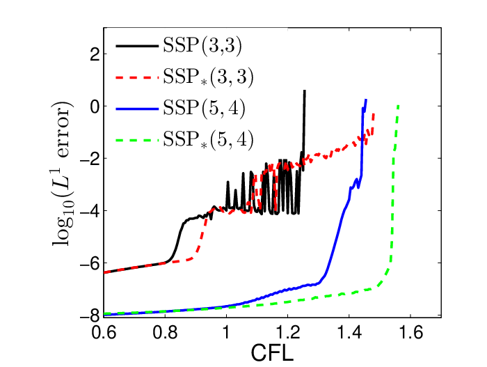
Fixing , we plot in Fig. 5.1 the error with respect to the CFL number. We see from the figure that, with our boundary treatment method, the errors for all the RK schemes remain small until a critical CFL number is reached, after which the error grows sharply. As expected, the RK schemes with negative coefficients give better stability than those without negative coefficients.
Next we take [5]
| (5.4) |
for which the exact solution is
| (5.5) |
For this definition of , the exact solution has a slope discontinuity for . A second discontinuity (this time in the solution) enters the computational domain from the inflow boundary at and persists until . It can be observed from Fig. 5.2 (left) that both types of discontinuities are well captured by our method for different RK methods. These results are comparable to those of the method in [5]. Note that the computational results remain good after the slope discontinuity passes through the right boundary; see Fig. 5.2 (right).


5.2 1D Burgers equation
The second problem is the Burgers equation
| (5.6) |
on the domain . For , this equation has the nonsmooth solution
| (5.7) |
In our computations, initial and boundary data are assigned according to this exact solution. Note that boundary conditions should be prescribed at both sides here since and .
With our boundary treatment method used at both boundaries, the computational results of the four RK schemes all agree well with the exact solution. To illustrate, solutions of the scheme with CFL=0.6 are presented in Fig. 5.3 for and . It can be seen that good results are obtained even after the discontinuity has entered from the right-hand boundary.


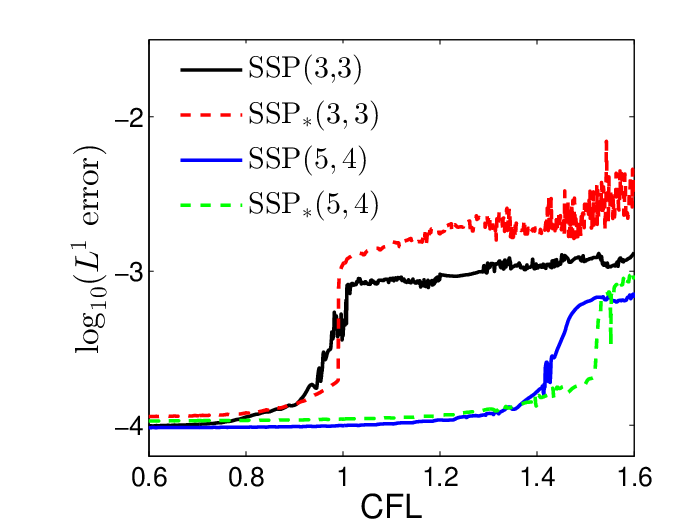
Next, we compare the errors at of the four RK schemes as the CFL number is varied. For this discontinuous, nonlinear problem, the plots in Fig. 5.4 show that the RK schemes with negative coefficients still give better stability than those without negative coefficients, though the advantage is not as pronounced as that for the smooth solution of the linear equation.
5.3 1D Euler equations
To conclude our experiments in 1D, we consider the 1D Euler equations
| (5.8) |
where and are the fluid density, velocity, pressure and total energy, respectively. The equation of state has the form
where is the specific heat ratio. The eigenvalues of the Jacobian matrix of the flux are and with giving the sound speed.
5.3.1 Accuracy test
We first test the accuracy of our method for a smooth solution on the domain [5]:
| (5.9) |
The initial condition is obtained by setting in the above solution. It can be directly verified that , and at both boundaries. Thus, two boundary conditions are needed at and one is required at . As in [5], we prescribe and at the left boundary:
and is given at the right boundary:
The errors and convergence orders of different RK schemes using a fixed CFL number of 0.6 are listed in Table 5.4 for this example. We see that for the third-order RK schemes, the convergence order is much larger than three for coarse meshes and that third-order convergence is achieved by taking very small -values. Similar to the linear problem, the convergence order is about five for the fourth-order RK schemes. As before, we conjecture that this is due to the error of the space discretization dominating over that of the time discretization.
| SSP(3,3) | ||||||||
| error | order | error | order | error | order | error | order | |
| 5.56e-6 | 1.62e-5 | 8.33e-6 | 2.31e-5 | |||||
| 1.89e-7 | 4.88 | 5.61e-7 | 4.85 | 2.75e-7 | 4.92 | 7.88e-7 | 4.87 | |
| 8.85e-9 | 4.42 | 2.38e-8 | 4.56 | 1.15e-8 | 4.58 | 3.06e-8 | 4.69 | |
| 6.42e-10 | 3.79 | 1.53e-9 | 3.96 | 7.26e-10 | 3.99 | 1.73e-9 | 4.14 | |
| 6.57e-11 | 3.29 | 1.51e-10 | 3.34 | 6.82e-11 | 3.41 | 1.56e-10 | 3.47 | |
| 7.75e-12 | 3.08 | 1.81e-11 | 3.06 | 7.82e-12 | 3.12 | 1.81e-11 | 3.11 | |
| SSP(5,4) | ||||||||
| error | order | error | order | error | order | error | order | |
| 5.33e-6 | 1.57e-5 | 7.02e-6 | 2.00e-5 | |||||
| 1.59e-7 | 5.07 | 4.91e-7 | 5.00 | 2.11e-7 | 5.06 | 6.31e-7 | 4.99 | |
| 5.00e-9 | 4.99 | 1.48e-8 | 5.05 | 6.61e-9 | 4.99 | 1.90e-8 | 5.05 | |
| 1.56e-10 | 5.00 | 4.13e-10 | 5.16 | 2.07e-10 | 5.00 | 5.32e-10 | 5.16 | |
| 5.01e-12 | 4.96 | 1.26e-11 | 5.03 | 6.33e-12 | 5.03 | 1.53e-11 | 5.12 |
5.3.2 Comparison with the method in [5]
We now verify our analysis of Section 4 where it was shown that order reduction arises when the method in [5] is applied to the nonlinear equations. To this end, we apply the SSP(3,3) RK method and the seventh-order WENO scheme to the 1D Euler equations with smooth solution (5.9). As in the computation for the linear scalar equation, the ideal WENO weights are used. Applying a fixed , we compare in Table 5.5 the errors of our method and that in [5]. It is clear that the designed seventh-order convergence is obtained for our method while the convergence order of the method in [5] is only about . This agrees with our analysis: our boundary treatment method maintains the accuracy of the interior spatial and time discretizations while the method in [5] introduces order reduction.
| our method | method in [6] | |||||||
|---|---|---|---|---|---|---|---|---|
| error | order | error | order | error | order | error | order | |
| 5.09e-6 | 1.31e-5 | 1.41e-5 | 4.52e-5 | |||||
| 4.36e-8 | 6.87 | 1.23e-7 | 6.73 | 2.16e-7 | 6.03 | 8.04e-7 | 5.81 | |
| 3.34e-10 | 7.03 | 1.00e-9 | 6.94 | 4.06e-9 | 5.73 | 1.49e-8 | 5.75 | |
| 3.54e-12 | 7.04 | 7.37e-12 | 7.08 | 7.62e-11 | 5.73 | 2.88e-10 | 5.69 |
5.3.3 Stability test
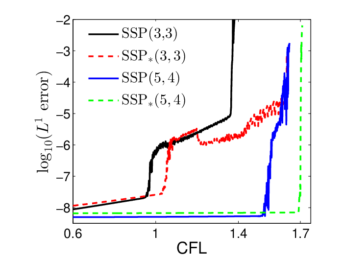
We conduct another test of the stability of our boundary treatment method for the Euler equations with smooth solution (5.9) by fixing and varying the CFL number. The corresponding errors are plotted in Fig. 5.5. Similar to the case of the linear equation, we see that the RK schemes with negative coefficients give better stability than those without negative coefficients. Furthermore, with our boundary treatment method, the error for all RK schemes remains small until a critical CFL number is reached, after which the error grows sharply.
5.3.4 Performance for shock interactions
To conclude, we test our method for the Euler equations on a problem with shocks that arise through the interaction of two blast waves [21, 5]. In this problem, the initial data are given by
| (5.10) |
and the boundaries are solid walls, namely, at and . As time evolves, there are multiple reflections of shocks and rarefactions off the walls. The shocks and rarefactions also interact with each other and with contact discontinuities. Similar to [5], we use second-order Taylor expansion at the boundary. The WENO type extrapolation in [5] is employed to avoid oscillations.
Fig. 5.6 gives a plot of our numerical solutions at . We see that the results of the and schemes coincide with each other. They also agree well with those of the method in [5]. These good results demonstrate the ability of our boundary treatment method to compute solutions to problems with complex shock interactions.


5.4 2D Euler equations
Though our method is illustrated only for 1D equations in Section 3, it can be directly extended to 2D problems [4]. In the following we examine our method for the 2D Euler equations
| (5.11) |
with
and equation of state . Here is the density, and are the velocities in and directions, is the total energy, is the pressure, and is the specific heat ratio. Specifically, we simulate the vortex problem with analytical solutions to the above 2D Euler equations as in [5]. In this problem, the mean flow is initially imposed with an isentropic vortex perturbation centered at in and in the temperature , no perturbation in the entropy :
Here , and is the vortex strength. The exact solution of this problem is a passive convection of the vortex with the mean velocity, i.e., . As in [5], we set the spatial domain and , and take boundary conditions from the exact solution whenever needed.
In the computation, we use the fifth-order WENO scheme [1] for the spatial discretization. The tangential derivative at the boundary is given by the exact solution and are computed by numerical differentiation. We take so that the signs of the eigenvalues at the boundary, and thereby the number of boundary conditions, do not change before the terminal time . The recently proposed method in [22] may be used to deal with the situation where the signs of the eigenvalues vary at the boundary. In this case, the errors are given in Table 5.6. It can be seen that the convergence orders of the computational results are generally larger than those of the four RK schemes. This may be due to the error of the spatial discretization dominating over that of the time discretization. These results verify the effectiveness of our method for 2D problems.
| SSP(3,3) | ||||||||
| error | order | error | order | error | order | error | order | |
| 6.17e-7 | 6.09e-6 | 1.00e-6 | 1.62e-5 | |||||
| 2.11e-8 | 4.87 | 3.94e-7 | 3.95 | 3.35e-8 | 4.91 | 1.69e-6 | 3.25 | |
| 7.83e-10 | 4.75 | 1.62e-8 | 4.61 | 1.61e-9 | 4.38 | 3.65e-7 | 2.21 | |
| 4.83e-11 | 4.02 | 1.76e-10 | 6.52 | 5.71e-11 | 4.82 | 8.21e-9 | 5.47 | |
| SSP(5,4) | ||||||||
| error | order | error | order | error | order | error | order | |
| 5.89e-7 | 4.71e-6 | 7.58e-7 | 8.38e-6 | |||||
| 1.93e-8 | 4.93 | 2.62e-7 | 4.17 | 2.42e-8 | 4.97 | 6.37e-7 | 3.72 | |
| 6.04e-10 | 5.00 | 7.52e-9 | 5.12 | 7.55e-10 | 5.00 | 4.87e-8 | 3.71 | |
| 2.82e-11 | 4.42 | 1.99e-10 | 5.24 | 3.06e-11 | 4.62 | 2.75e-10 | 7.47 |
6 Conclusions and remarks
In this paper, we examine the finite difference boundary treatment method proposed in our previous work [4] for the case of explicit high-order SSP RK schemes applied to hyperbolic conservation laws. Our spatial discretization uses a WENO scheme on a Cartesian mesh where the corresponding downwind scheme is applied in the case of negative coefficients. We show that our method applies to general SSP RK schemes with/without negative coefficients. Our method preserves the accuracy of the RK schemes and has good stability. These nice properties are verified on linear and nonlinear problems using third- and fourth-order RK schemes with and without negative coefficients. In addition, when boundary conditions are present and our boundary treatment method is used, the SSP RK schemes with negative coefficients still allow for larger time steps than those with all nonnegative coefficients. In this regard, the boundary treatment method in [4] is an effective supplement to SSP RK schemes with/without negative coefficients for initial-boundary value problems of conservation laws.
It should be remarked that the key point of our method is to use the RK scheme itself at the boundary, instead of imposing intermediate boundary conditions as in [5, 6]. The boundary conditions in those previous works [5, 6] are derived only for RK schemes up to third order while our method applies to RK schemes of arbitrary order. In addition, we show the equivalence of our method and that in [5, 6] for linear problems and the case of the third-order SSP RK scheme. On the other hand, for nonlinear equations, there exist difference terms of between the two methods, which result in order reduction for the method in [5, 6]. These results have been numerically verified as well.
Acknowledgements
This work was supported by the National Foreign Experts Project of China (No. G20190001349) and the National Natural Science Foundation of China (No. 11801030, No. 11861131004).
Appendix
This appendix gives the computation of at ghost points . As for , is approximated with the fifth-order Taylor expansion at the boundary point :
| (6.1) |
where denotes a -th order approximation of the spatial derivative . Next, we compute for . To this end, we apply the second stage of the RK solver (2.3) for at the boundary point :
| (6.2) |
Notice that
Substituting these into (6.2), we obtain an approximation of and denote it by . Observe that the error between and defined by (6.2) is .
Taking derivatives with respect to on both sides of (6.2) yields
| (6.3) |
With approximations
can be computed with (6.3) and the resulting solution is a fourth-order approximation of .
Furthermore, we simply approximate for by using a -th order extrapolation with at interior points. In this way, we obtain for with accuracy of order . Then, for can be computed by (6.1) with fifth-order accuracy. Having at the ghost points, we can then evolve from to using the interior difference scheme.
References
- [1] C.-W. Shu and S. Osher. Efficient implementation of essentially nonoscillatory shockcapturing schemes. J. Comput. Phys., 77(2):439–471, 1988.
- [2] C.-W. Shu. Total-variation-diminishing time discretizations. SIAM J. Sci. Statist. Comput., 9(6):1073–1084, 1988.
- [3] S. Gottlieb, C.-W. Shu, and E. Tadmor. Strong stability-preserving high-order time discretization methods. SIAM Review, 43(1):89–112, 2001.
- [4] W. Zhao and J. Huang. Boundary treatment of implicit-explicit Runge-Kutta method for hyperbolic systems with source terms. arXiv preprint arXiv:1908.01027, 2019.
- [5] S. Tan and C.-W. Shu. Inverse Lax-Wendroff procedure for numerical boundary conditions of conservation laws. Journal of Computational Physics, 229(21):8144–8166, 2010.
- [6] S. Tan, C. Wang, C.-W. Shu, and J. Ning. Efficient implementation of high order inverse Lax-Wendroff boundary treatment for conservation laws. J. Comput. Phys., 231(6):2510–2527, 2012.
- [7] S. Gottlieb and C.-W. Shu. Total variation diminishing Runge-Kutta schemes. Math. Comp., 67:73–85, 1998.
- [8] S. J. Ruuth and R. J. Spiteri. Two barriers on strong-stability-preserving time discretization methods. J. Sci. Comput., 17(1-4):211–220, 2002.
- [9] R. J. Spiteri and S. J. Ruuth. A new class of optimal high-order strong-stability-preserving time discretization methods. SIAM J. Numer. Anal., 40(2):469–491, 2002.
- [10] S. J. Ruuth and R. J. Spiteri. High-order strong-stability-preserving Runge-Kutta methods with downwind-biased spatial discretizations. SIAM J. Numer. Anal., 42(3):974–996, 2004.
- [11] S. J. Ruuth. Global optimization of explicit strong-stability-preserving Runge-Kutta methods. Math. Comput., 75(253):183–207, 2005.
- [12] S. Gottlieb and S. J. Ruuth. Optimal strong-stability-preserving time-stepping schemes with fast downwind spatial discretizations. J. Sci. Comput., 27(1-3):289–303, 2006.
- [13] M. H. Carpenter, D. Gottlieb, S. Abarbanel, and W.-S. Don. The theoretical accuracy of Runge-Kutta time discretizations for the initial boundary value problem: A study of the boundary error. SIAM Journal on Scientific Computing, 16(6):1241–1252, 1995.
- [14] S. Abarbanel, D. Gottlieb, and M. H. Carpenter. On the removal of boundary errors caused by Runge–Kutta integration of nonlinear partial differential equations. SIAM Journal on Scientific Computing, 17(3):777–782, 1996.
- [15] D. Pathria. The correct formulation of intermediate boundary conditions for Runge–Kutta time integration of initial boundary value problems. SIAM Journal on Scientific Computing, 18(5):1255–1266, 1997.
- [16] T. J. Poinsot and S. K. Lele. Boundary conditions for direct simulations of compressible viscous flows. J. Comput. Phys., 101:104–129, 1992.
- [17] Y. Hadjimichael. Perturbed Strong Stability Preserving Time-Stepping Methods For Hyperbolic PDEs. PhD thesis, King Abdullah University of Science and Technology, 2017.
- [18] G.-S. Jiang and C.-W. Shu. Efficient implementation of weighted ENO schemes. J. Comput. Phys., 126:202–228, 1996.
- [19] D. S. Balsara and C.-W. Shu. Monotonicity preserving weighted essentially non-oscillatory schemes with increasingly high order of accuracy. J. Comput. Phys., 160:405–452, 2000.
- [20] Y. Shen and G. Zha. A robust seventh-order WENO scheme and its applications. 46th AIAA Aerospace Sciences Meeting and Exhibit, doi:10.2514/6.2008-757, 2008.
- [21] P. Woodward and P. Colella. The numerical simulation of two-dimensional fluid flow with strong shocks. J. Comput. Phys., 54:115–173, 1984.
- [22] J. Lu, C.-W. Shu, S. Tan, and M. Zhang. An inverse Lax-Wendroff procedure for hyperbolic conservation laws with changing wind direction on the boundary. preprint, http://www.dam.brown.edu/people/shu/pub.html.