Predicting novel superconducting hydrides using machine learning approaches
Abstract
The search for superconducting hydrides has, so far, largely focused on finding materials exhibiting the highest possible critical temperatures (). This has led to a bias towards materials stabilised at very high pressures, which introduces a number of technical difficulties in experiment. Here we apply machine learning methods in an effort to identify superconducting hydrides which can operate closer to ambient conditions. The output of these models informs subsequent crystal structure searches, from which we identify stable metallic candidates prior to performing electron-phonon calculations to obtain . Hydrides of alkali and alkaline earth metals are identified as especially promising; of particular note, a of up to 115 K is calculated for RbH12 at 50 GPa, which extends the operational pressure-temperature range occupied by hydride superconductors towards ambient conditions.
I Introduction
While hydrogen is predicted to be a room-temperature superconductor at very high pressures Ashcroft 1968, metal hydrides, in which the hydrogen atoms are “chemically pre-compressed”, are predicted to exhibit similar behaviour in experimentally-accessible regimes Gilman 1971; Ashcroft 2004. In recent years, potential superconductivity has been investigated in many compressed hydrides, including scandium Durajski and Szczesniak 2014, sulfur Duan et al. 2014; Drozdov et al. 2015; Errea et al. 2015, yttrium Kim et al. 2009; Li et al. 2015; Liu et al. 2017a; Peng et al. 2017; Heil et al. 2019; Troyan et al. 2019; Kong et al. 2019; Shipley et al. 2020, calcium Wang et al. 2012, actinium Semenok et al. 2018a, thorium Kvashnin et al. 2018a, pnictogen Fu et al. 2016, praseodymium Zhou et al. 2019a, cerium Salke et al. 2019; Li et al. 2019, neodymium Zhou et al. 2019b, lanthanum Liu et al. 2017a; Peng et al. 2017; Somayazulu et al. 2019; Drozdov et al. 2019; Shipley et al. 2020; Kruglov et al. and iron hydrides Majumdar et al. 2017; Kvashnin et al. 2018b; Heil et al. 2018. Several reviews summarising recent developments in the field are available Duan et al. 2017; Zurek and Bi 2019; Flores-Livas et al. 2019; Boeri and Bachelet 2019; Pickard et al. 2020; Bi et al. 2019. Inspired by known superconductors, researchers have also attempted to increase by chemical means; replacing atoms in known structures and assessing stability and superconductivity Chang et al. 2019, doping known binaries with more electronegative elements to make ternary hydrides Sun et al. 2019, and mapping alchemical phase diagrams Heil and Boeri 2015.
Experimental measurements of superconductivity in high-pressure hydrides have helped to address several misconceptions about conventional superconductivity, fuelling hope that it may be achieved at ambient temperature and waving a definitive farewell to the Cohen-Anderson limit Cohen and Anderson 1972. The associated theoretical studies have demonstrated that the crystal structures and superconducting properties of real materials can now be accurately predicted from first principles.
In this work, we train machine learning models on a set of literature data for superconducting binary hydrides. Machine learning has previously been used in modelling hydride superconductors, with a focus on predicting the maximum obtainable critical temperature for a given composition Semenok et al. 2018b. However, on examination of the literature (see Fig. 1), it becomes apparent that the pursuit of superconductivity close to ambient conditions is as much about reducing the required pressure as it is about increasing the critical temperature. This is especially important given that working at high pressure can often present a far greater experimental challenge than working at low temperature. In this work, we therefore model critical temperature and operational pressure on an equal footing. Our models are used to inform the choice of composition for crystal structure searches and subsequent electron-phonon calculations, with the aim of extending the operation of hydride superconductors towards ambient conditions.
II Trends in Hydrides

A large amount of computational - and some experimental - data for the binary hydrides is available in the literature Geballe et al. 2018; Troyan et al. 2019; Errea et al. 2019; Heil et al. 2019; Kong et al. 2019; Xie et al. 2014; Zhou et al. 2012; Yu et al. 2014; Lonie et al. 2013; Tse et al. 2009; Semenok et al. 2018a; Kvashnin et al. 2018a; Wang et al. 2012; Zemła et al. 2019; Kruglov et al. 2018; Feng et al. 2015; Gu et al. 2017; Durajski and Szczesniak 2014; Esfahani et al. 2017; Wei et al. 2016; Zhou et al. 2019a; Liu et al. 2017b; Semenok et al. 2019; Peng et al. 2017; Liu et al. 2017a; Zarifi et al. 2018; Shanavas et al. 2016; Li et al. 2017a; Kresin 2018; Semenok et al. 2018b; Liu et al. 2015; Ohlendorf and Wicke 1979; Chen et al. 2014; Gao et al. 2013; Zhuang et al. 2017a; Yu et al. 2015; Spitsyn et al. 1982; Li et al. 2017b; Kvashnin et al. 2018b; Liu et al. 2016; Liu et al. 2015; Ye et al. 2018; Skoskiewicz et al. 1974; Li and Peng 2017; Errea et al. 2014; Tanaka et al. 2017; Hu et al. 2013; Wei et al. 2013; Hou et al. 2015; Li et al. 2016; Szczesniak and Durajski 2013; Hooper et al. 2013; Liu et al. 2015; Yao et al. 2007; Zhuang et al. 2017b; Eremets et al. 2008; Li et al. 2010; Jin et al. 2010; Liu et al. 2018; Drozdov et al. 2018; Somayazulu et al. 2019; Drozdov et al. 2019; Li et al. 2015 (values from these references form our dataset, shown in Fig. 1). In some subsets of hydrides certain material properties show a simple dependence on the properties of the non-hydrogen element. For example, in the alkaline earth hydrides the van der Waals radius of the ion is well correlated with the metallization pressure Zhang et al. 2010. However, obtaining strong electron-phonon coupling at low pressures is, in general, a more complicated process; simple correlations between composition and operational pressure or critical temperature are therefore absent in the dataset as a whole. We look at more complicated trends by constructing machine learning models of critical temperature and operational pressure which take as input a set of easily-obtained material descriptors. For a particular element E and corresponding binary hydride EHn these descriptors are
- •
hydrogen content ()
- •
van der Waals radius of E
- •
atomic number of E
- •
mass number of E
- •
numbers of , , and electrons in the (atomic) electron configuration of E
Once constructed, we apply the model to all materials with the chemical composition EHn, where E is any element in the periodic table and 11 1 A maximum of 31 hydrogens per atom was chosen to avoid over-extrapolation from the dataset (where the maximum is 16).. From these, the materials which are predicted to exhibit superconductivity closest to ambient conditions serve as a guide for searches for new binary hydrides.
II.1 Neural network
We train a fully-connected neural network (using the Keras frontend to the Tensorflow machine-learning library Chollet et al. 2015; Abadi et al. 2015), with the topology shown in Fig. 2, on the dataset shown in Fig. 1. The squared absolute error between the predicted and literature values serves as our cost function, which we minimize using the Adam stochastic optimizer Kingma and Ba 2014. The input (and expected output) data is positive definite and therefore has a non-zero mean and is not normally distributed, prompting the use of self-normalizing activation functions Klambauer et al. 2017; Clevert et al. 2015 to improve training behaviour. Since the number of data points is comparable to the number of parameters in our network, the risk of over-fitting becomes significant. To mitigate this, we split the data into a randomly selected validation set (consisting of 25% of the initial data points) and a training set (consisting of the other 75%). Once the model starts over-fitting to the training data the validation set error starts to increase, allowing us to choose the model parameters from the training epoch for which the validation set error is minimal. We cross-validate the results by repeating this process 64 times and averaging the predictions - this is an approximation of leave--out cross-validation with of the dataset. We also apply regularization to the parameters in the intermediate dense nodes to decrease the propensity for over-fitting, improving the convergence of this cross-validation scheme.
II.2 Model behaviour
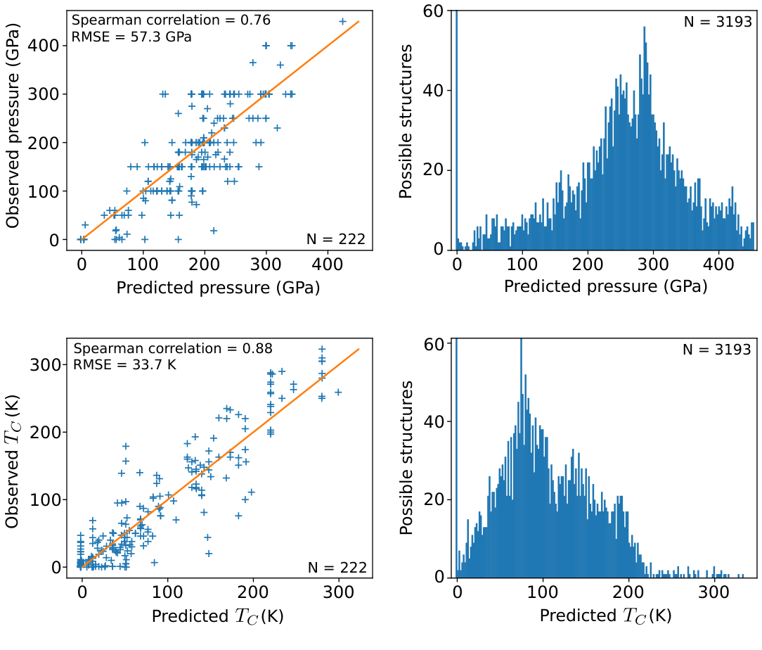
The basic behaviour of the machine learning model is shown in Fig. 3. We see that it achieves reasonable correlation with the literature values and predicts sensible pressures and temperatures for unseen materials. To gain insight into properties which favour ambient-condition superconductivity we define a measure of distance . This distance decreases as we move towards ambient conditions from the pressure-temperature region containing the known hydrides (see Fig. 1). In Fig. 4 we plot the distribution of material properties for the 10% of hydrides predicted to exhibit superconductivity closest to ambient conditions (i.e., the 10% with lowest ). We can see that the model predicts the heavy alkali and alkaline earth metal hydrides to be the best candidates, with the number of close-to-ambient materials then decreasing as we go across each period. The distribution of the number of hydrogen atoms is more uniform, suggesting it is necessary to consider a range of different stoichiometries for each composition. These conclusions are reinforced by the construction of a simple linear regression model sup, which reproduces the general trends exhibited by the machine learning model (but, unsurprisingly, exhibits worse correlation with the literature values). The predicted optimal (minimum ) hydride compositions from the machine learning model are shown for each element of the periodic table in Fig. 5.
We note that the points included in our dataset will be of varying quality, come from different research groups, and are of both experimental and theoretical origin. The majority are theoretical and calculated within the harmonic approximation. Although it has been shown that anharmonicity can affect the calculated critical temperature for hydrides Errea et al. 2013; Errea et al. 2015, there is insufficient data in the literature to build a model exclusively from anharmonic results. However, since we only seek to extract general trends, which will serve simply to inform areas of focus for structure searching, the dataset is sufficient for our purposes.

III Structure searching
The models constructed in the previous section point towards the alkali and alkaline earth metal hydrides as some of the best candidates for superconductivity near ambient conditions. From these, we studied caesium and rubidium hydrides; these systems were chosen due to their predicted proximity to superconductivity at ambient conditions (see Figs. 4 and 5) and the fact that they have not been studied extensively in the past, unlike the hydrides of other elements in these two groups. Caesium and rubidium polyhydrides have been studied previously using structure searching methods in Refs. Shamp et al. 2012 and Hooper and Zurek 2012, respectively, although potential superconductivity was not investigated in either case.
Our structure searching calculations were performed using ab initio random structure searching (AIRSS) Pickard and Needs 2011; Needs and Pickard 2016 and the plane-wave pseudopotential code castep Clark et al. 2005. Since our models suggest that a wide range of stoichiometries should be considered, convex hulls were constructed using AIRSS and qhull Barber et al. 1996 in order to identify those which are stable at 50, 100 and 200 GPa sup. The Perdew-Burke-Ernzerhof (PBE) generalised gradient approximation Perdew et al. 1996, castep QC5 pseudopotentials, a 400 eV plane-wave cut-off and a -point spacing of 0.05 Å-1 were used in all searches. The Cs-H convex hulls calculated in this work at 100 and 200 GPa both partially agree with the hull calculated at 150 GPa in Ref. Shamp et al. 2012. Once stable stoichiometries had been identified, additional AIRSS searches for RbH3, RbH5, RbH9, RbH11, RbH12, CsH5, CsH7, CsH13 and CsH15 using the same parameters and pseudopotentials were performed at 100 and 200 GPa.
IV Selecting candidate structures
For each selected stoichiometry, the enthalpy was calculated as a function of pressure for the most stable structures arising from the AIRSS search. These geometry optimisations were performed using quantum espresso Giannozzi et al. 2009; Giannozzi et al. 2017, the PBE functional, a 950 eV cut-off, ultrasoft pseudopotentials sup and a -point spacing of 0.02 Å-1. The electronic density of states (DOS) at the Fermi energy was also evaluated for each structure at 50 GPa and 150 GPa in order to identify metallic structures. We were then able to limit our interest to structures which were both energetically competitive (according to the enthalpy plots) and had a considerable DOS at the Fermi energy in the low-pressure region (25-125 GPa). Full lists of the competitive structures predicted here are available, along with the enthalpy plots and DOS values, in the supplementary material sup. The remaining candidates, for which electron-phonon coupling calculations were performed, include -RbH12, -RbH12, and various CsH7 and RbH3 structures (see Table 1).
V Electron-phonon coupling and superconductivity
The Hamiltonian of a coupled electron-phonon system is given by
| (1) |
In this work, we calculate the electronic Kohn-Sham eigenvalues , phonon frequencies , and electron-phonon coupling constants appearing in from first-principles using density functional perturbation theory (DFPT) as implemented in the quantum espresso code Giannozzi et al. 2009; Giannozzi et al. 2017. The resulting Hamiltonian is then treated within Migdal-Eliashberg theory Migdal 1958; Eliashberg 1960; Sanna et al. 2018 where we solve the Eliashberg equations using the elk code elk. This gives us the superconducting gap as a function of temperature, from which we obtain a prediction for .
To carry out these calculations, we use the PBE functional, the same ultrasoft pseudopotentials as in the geometry optimisations, an 820 eV plane-wave cut-off, and a -point grid with a spacing of Å-1 (e.g., a grid for a 26-atom unit cell of RbH12). Two separate -point grids are used (of and times the size of the -point grid, respectively), allowing us to determine the optimal double-delta smearing width necessary to calculate the critical temperature Wierzbowska et al. 2005; Shipley et al. 2020.
Electron-phonon calculations were performed for a range of competitive RbH12, CsH7 and RbH3 structures predicted in this work and the results are shown in Table 1. The highest- results arise from structures with a cage-like arrangement of hydrogen atoms surrounding a central non-hydrogen element. The electronic states that originate from these cages are near the Fermi level, and are strongly coupled together by cage vibrations. This provides the phonon-mediated pairing mechanism necessary for conventional superconductivity. Combined with a high average phonon frequency, owing to the light mass of the hydrogen atoms, this results in a high critical temperature (c.f the Allen-Dynes equation Allen and Dynes 1975). This can be seen directly by looking at the Eliashberg function, shown in Fig. 6, for two illustrative structures from Table 1. The enhanced high-frequency portion of the Eliashberg function for the high- cage-like RbH12 structure is apparent. In contrast, strong electron-phonon coupling is absent at high phonon frequencies for states near the Fermi level in the layered RbH3 structure, leading to a negligible . It is perhaps unsurprising that our machine learning model suggests such compositions, despite their resulting unfavorable structures, as it is trained on mostly cage-like structures. As a result, the model may implicitly assume that compositions it is given will behave as if they adopt cage-like arrangements, leading to an overestimation of . Despite this, most of the structures found are high- cage-like superconductors, of which -RbH12 is particularly interesting due to its location in Fig. 1.
Supplementing structure searching techniques with predictions from machine learning has allowed us to target novel regions of pressure-temperature space. We have therefore been able to identify low-pressure hydride superconductors without having to perform a large number of expensive electron-phonon calculations. It can be seen from Fig. 1 that the hydrides predicted in this work are biased towards ambient conditions when compared to the dataset as a whole.
| Stoichiometry | Space group | Pressure (GPa) | (K) |
|---|---|---|---|
| RbH12 | 50 | 108 | |
| RbH12 | 100 | 129 | |
| RbH12 | 150 | 133 | |
| RbH12 | 100 | 82 | |
| RbH12 | 50 | 115 | |
| RbH12 | 100 | 119 | |
| RbH12 | 150 | 126 | |
| CsH7 | 100 | 90 | |
| CsH7 | 100 | 34 | |
| CsH7 | 100 | 33 | |
| CsH7 | 100 | 10 | |
| CsH7 | 100 | 5 | |
| CsH7 | 100 | 89 | |
| RbH3 | 100 | 0 | |
| RbH3 | 100 | 0 |

VI Testing potential screening techniques for high- candidates
In this work we also tested two potential methods for cheaply estimating ordering between structures. Good superconductivity in hydrides generally requires hydrogenic states close to the Fermi level, which (as exemplified by the findings of this work) often means favouring cage-like structures and avoiding structures with molecular-character H2 units. It is therefore possible that the hydrogen-derived DOS normalised by the total DOS at the Fermi energy, , may give some indication of whether a particular structure will exhibit high- superconductivity. Here we also consider the hydrogen-derived electron-phonon coupling estimates () from Gaspari-Gyorffy theory Gaspari and Gyorffy 1972 and test whether these two quantities could provide a method for ranking different structures (of the same stoichiometry and at the same pressure) before performing expensive electron-phonon calculations. We implemented Gaspari-Gyorffy theory within the elk code elk. The basics of this theory and its use here are explained in Appendix A.
The calculated values for the structures predicted and studied in this work allowed us to directly assess these potential screening methods. We observe that correctly predicts the ordering for the RbH12 structures at fixed pressure, as was the case for the LaH10 and YH10 systems on which preliminary tests were performed sup. The two quantities tested here often predict the same general trends, but the DOS ratio is cheaper to calculate since it can be obtained using a pseudopotential code. Unfortunately, appears to be much less predictive for the CsH7 structures and the performance of is also mixed sup. The use of these quantities for screening applications therefore requires further investigation and testing in a wider variety of systems.
VII Conclusions
Having identified the need to reduce the operational pressure of hydride superconductors, we searched for crystal structures which would exhibit superconductivity in novel regions of pressure-temperature space. We found that guiding structure searching techniques using a machine learning model allowed us to target the most promising regions. Specifically, we constructed models of critical temperature and operational pressure trained on the available theoretical and experimental results for binary hydride superconductors. Several novel systems were identified as promising superconductors closer to ambient conditions; here we focused on Cs and Rb hydrides, using AIRSS to identify stable stoichiometries and predict crystal structures. Other promising candidates included Ca, Sr, Ba, Ra, Ac, Th, La and Sc hydrides, most of which had already been theoretically studied to some extent Wang et al. 2012; Tanaka et al. 2017; Bi et al. 2019; Hooper et al. 2013; Semenok et al. 2018a; Kvashnin et al. 2018a; Semenok et al. 2019; Liu et al. 2017a; Peng et al. 2017; Liu et al. 2018; Kruglov et al.; Durajski and Szczesniak 2014. Critical temperatures of energetically-competitive candidate structures were then calculated from first principles using DFPT. A of up to 115 K was calculated for RbH12 at 50 GPa, which represents a significant extension towards ambient-condition superconductivity from our dataset.
Acknowledgements
We thank Po-Hao Chang for useful discussions regarding Gaspari-Gyorffy theory. M.J.H. acknowledges the EPSRC Centre for Doctoral Training in Computational Methods for Materials Science for funding under grant number EP/L015552/1. A.M.S. acknowledges funding through an EPSRC studentship. R.J.N. is supported by EPSRC under Critical Mass Grant EP/P034616/1 and the UKCP consortium grant EP/P022596/1. We are grateful for computational support from the UK national high performance computing service, ARCHER, for which access was obtained via the UKCP consortium and funded by EPSRC grant ref EP/P022561/1. This work was also performed using resources provided by the Cambridge Service for Data Driven Discovery (CSD3) operated by the University of Cambridge Research Computing Service ( www.csd3.cam.ac.uk), provided by Dell EMC and Intel using Tier-2 funding from the EPSRC (capital grant EP/P020259/1), and DiRAC funding from the STFC (www.dirac.ac.uk).
Appendix A Gaspari-Gyorffy theory
McMillan McMillan 1968 showed that for strong-coupled superconductors the electron-phonon coupling constant, , can be expressed as
| (2) |
can also be reformatted as
where is the so-called Hopfield parameter. Hopfield was one of the first to stress the importance of the local environment in determining Hopfield 1969. In situations where we have nearly perfect separation of vibrational modes into those of different atomic character (such as we may see in hydrides) we can write
| (3) |
where is the atom type.
The quantity appearing in Eq. 2 can be approximated using Gaspari-Gyorffy (GG) theory Gaspari and Gyorffy 1972. Recent work has emerged using this theory for metal hydrides under high pressure Papaconstantopoulos et al. 2015; Chang et al. 2019 despite it originally being designed for elemental transition metals. The theory, based on the rigid muffin-tin approximation (RMTA), relies on several approximations Papaconstantopoulos et al. 2015 and allows us to reformulate the electron-phonon interaction in terms of phase shifts for a scattering potential. A self-consistent DOS calculation is thus all that is required to calculate for each atom type and hence obtain . The GG equation is
| (4) |
where is the free-scatterer DOS given by
| (5) |
and the are the scattering phase shifts. Here is the muffin-tin radius associated with atom type and is the scattering solution of the Schrödinger equation. The phase shifts, which characterise the long-distance behaviour of the wavefunction, can be written in terms of the logarithmic derivative of the radial wavefunction
| (6) |
where , is the logarithmic derivative, are spherical Bessel functions and are Neumann functions. We can therefore directly calculate the logarithmic derivative and use Eq. 6 to obtain the phase shifts Sakurai and Napolitano 2017.
Since is often considerably smaller for hydrogen than for the other components, it is clear from Eq. 3 that the hydrogen atoms can provide a considerable fraction of even if the Hopfield parameter of the other atom type is similar in magnitude. Calculating can therefore, in some cases, provide a cheap screening method for identifying potential high- hydrides. In particular, the average phonon frequencies for different structures are often similar when considering the same stoichiometry at the same pressure. If the average phonon frequencies are assumed to be exactly equivalent in such cases, we then arrive at a potential way of estimating ordering between structures, simply by considering . It is in this context that we assess the utility of GG theory in this work.
References
- Ashcroft (1968) N. W. Ashcroft, Phys. Rev. Lett. 21, 1748 (1968).
- Gilman (1971) J. Gilman, Physical Review Letters 26, 546 (1971).
- Ashcroft (2004) N. W. Ashcroft, Phys. Rev. Lett. 92, 187002 (2004).
- Durajski and Szczesniak (2014) A. P. Durajski and R. Szczesniak, Supercond. Sci. and Tech. 27, 115012 (2014).
- Duan et al. (2014) D. Duan, Y. Liu, F. Tian, D. Li, X. Huang, Z. Zhao, H. Yu, B. Liu, W. Tian, and T. Cui, Nature - Scientific Reports 4, 6968 (2014).
- Drozdov et al. (2015) A. P. Drozdov, M. I. Eremets, I. A. Troyan, V. Ksenofontov, and S. I. Shylin, Nature 525, 73 (2015).
- Errea et al. (2015) I. Errea, M. Calandra, C. J. Pickard, J. Nelson, R. J. Needs, Y. Li, H. Liu, Y. Zhang, Y. Ma, and F. Mauri, Phys. Rev. Lett. 114, 157004 (2015).
- Kim et al. (2009) D. Y. Kim, R. H. Scheicher, and R. Ahuja, Phys. Rev. Lett. 103, 077002 (2009).
- Li et al. (2015) Y. Li, J. Hao, H. Liu, J. S. Tse, Y. Wang, and Y. Ma, Scientific Reports 5, 9948 (2015).
- Liu et al. (2017a) H. Liu, I. I. Naumov, R. Hoffmann, N. W. Ashcroft, and R. J. Hemley, Proc. Nat. Acad. Sci. 114, 6990 (2017a).
- Peng et al. (2017) F. Peng, Y. Sun, C. J. Pickard, R. J. Needs, Q. Wu, and Y. Ma, Phys. Rev. Lett. 119, 107001 (2017).
- Heil et al. (2019) C. Heil, S. di Cataldo, G. B. Bachelet, and L. Boeri, Phys. Rev. B 99, 220502(R) (2019).
- Troyan et al. (2019) I. A. Troyan, D. V. Semenok, A. G. Kvashnin, A. G. Ivanova, V. B. Prakapenka, E. Greenberg, A. G. Gavriliuk, I. S. Lyubutin, V. V. Struzhkin, and A. R. Oganov, arXiv preprint arXiv:1908.01534 (2019).
- Kong et al. (2019) P. P. Kong, V. S. Minkov, M. A. Kuzovnikov, S. P. Besedin, A. P. Drozdov, S. Mozaffari, L. Balicas, F. F. Balakirev, V. B. Prakapenka, E. Greenberg, D. A. Knyazev, and M. I. Eremets, arXiv preprint arXiv:1909.10482 (2019).
- Shipley et al. (2020) A. M. Shipley, M. J. Hutcheon, M. S. Johnson, C. J. Pickard, and R. J. Needs, arXiv:2001.05305 (2020).
- Wang et al. (2012) H. Wang, J. S. Tse, K. Tanaka, T. Iitaka, and Y. Ma, Proc. Nat. Acad. Sci. 109, 6463 (2012).
- Semenok et al. (2018a) D. V. Semenok, A. G. Kvashnin, I. A. Kruglov, and A. R. Oganov, J. Phys. Chem. Lett. 9, 1920 (2018a).
- Kvashnin et al. (2018a) A. G. Kvashnin, D. V. Semenok, I. A. Kruglov, I. A. Wrona, and A. R. Oganov, ACS Appl. Mater. Interfaces 10, 43809 (2018a).
- Fu et al. (2016) Y. Fu, X. Du, L. Zhang, F. Peng, M. Zhang, C. J. Pickard, R. J. Needs, D. J. Singh, W. Zheng, and Y. Ma, Chem. Mater. 28, 1746 (2016).
- Zhou et al. (2019a) D. Zhou, D. Semenok, D. Duan, H. Xie, X. Huang, W. Chen, X. Li, B. Liu, A. R. Oganov, and T. Cui, arXiv preprint arXiv:1904.06643 (2019a).
- Salke et al. (2019) N. P. Salke, M. M. D. Esfahani, Y. Zhang, I. A. Kruglov, J. Zhou, Y. Wang, E. Greenberg, V. B. Prakapenka, J. Liu, A. R. Oganov, and J.-F. Lin, Nature Communications 10, 1 (2019).
- Li et al. (2019) X. Li, X. Huang, D. Duan, C. J. Pickard, D. Zhou, H. Xie, Q. Zhuang, Y. Huang, Q. Zhou, B. Liu, and T. Cui, Nature Communications 10, 3461 (2019).
- Zhou et al. (2019b) D. Zhou, D. V. Semenok, H. Xie, A. I. Kartsev, A. G. Kvashnin, X. Huang, D. Duan, A. R. Oganov, and T. Cui, arXiv preprint arXiv:1908.08304 (2019b).
- Somayazulu et al. (2019) M. Somayazulu, M. Ahart, A. K. Mishra, Z. M. Geballe, M. Baldini, Y. Meng, V. V. Struzhkin, and R. J. Hemley, Phys. Rev. Lett. 122, 027001 (2019).
- Drozdov et al. (2019) A. P. Drozdov, P. P. Kong, V. S. Minkov, S. P. Besedin, M. A. Kuzovnikov, S. Mozaffari, L. Balicas, F. F. Balakirev, D. E. Graf, V. B. Prakapenka, E. Greenberg, D. A. Knyazev, M. Tkacz, and M. I. Eremets, Nature 569, 528 (2019).
- (26) I. A. Kruglov, D. V. Semenok, H. Song, R. Szczesniak, I. A. Wrona, R. Akashi, M. M. D. Esfahani, D. Duan, T. Cui, A. G. Kvashnin, and A. R. Oganov, .
- Majumdar et al. (2017) A. Majumdar, J. S. Tse, M. Wu, and Y. Yao, Phys. Rev. B 96, 201107 (2017).
- Kvashnin et al. (2018b) A. G. Kvashnin, I. A. Kruglov, D. V. Semenok, and A. R. Oganov, J. Phys. Chem. C 122, 4731 (2018b).
- Heil et al. (2018) C. Heil, G. B. Bachelet, and L. Boeri, Physical Review B 97, 214510 (2018).
- Duan et al. (2017) D. Duan, Y. Liu, Y. Ma, Z. Shao, B. Liu, and T. Cui, Natl. Sci. Rev 4, 121 (2017).
- Zurek and Bi (2019) E. Zurek and T. Bi, J. Chem. Phys. 150, 050901 (2019).
- Flores-Livas et al. (2019) J. A. Flores-Livas, L. Boeri, A. Sanna, G. Profeta, R. Arita, and M. I. Eremets, arXiv preprint arXiv:1905.06693 (2019).
- Boeri and Bachelet (2019) L. Boeri and G. B. Bachelet, J. Phys: Condens. Matt. 31, 234002 (2019).
- Pickard et al. (2020) C. J. Pickard, I. Errea, and M. I. Eremets, Annual Review of Condensed Matter Physics 11, 57 (2020).
- Bi et al. (2019) T. Bi, N. Zarifi, T. Terpstra, and E. Zurek (Elsevier, 2019).
- Chang et al. (2019) P.-H. Chang, S. Silayi, D. Papaconstantopoulos, and M. Mehl, Journal of Physics and Chemistry of Solids , 109315 (2019).
- Sun et al. (2019) Y. Sun, J. Lv, Y. Xie, H. Liu, and Y. Ma, Phys. Rev. Lett. 123, 097001 (2019).
- Heil and Boeri (2015) C. Heil and L. Boeri, Phys. Rev. B 92, 060508 (2015).
- Cohen and Anderson (1972) M. L. Cohen and P. W. Anderson, in AIP Conference Proceedings, Vol. 4 (AIP, 1972) pp. 17–27.
- Semenok et al. (2018b) D. V. Semenok, I. A. Kruglov, A. G. Kvashnin, and A. R. Oganov, arXiv preprint arXiv:1806.00865 (2018b).
- Geballe et al. (2018) Z. M. Geballe, H. Liu, A. K. Mishra, M. Ahart, M. Somayazulu, Y. Meng, M. Baldini, and R. J. Hemley, Angewandte Chemie International Edition 57, 688 (2018).
- Errea et al. (2019) I. Errea, F. Belli, L. Monacelli, A. Sanna, T. Koretsune, T. Tadano, R. Bianco, M. Calandra, R. Arita, F. Mauri, and J. A. Flores-Livas, arXiv preprint arXiv:1907.11916 (2019).
- Xie et al. (2014) Y. Xie, Q. Li, A. R. Oganov, and H. Wang, Acta Crystallographica Section C 70, 104 (2014).
- Zhou et al. (2012) D. Zhou, X. Jin, X. Meng, G. Bao, Y. Ma, B. Liu, and T. Cui, Phys. Rev. B 86, 014118 (2012).
- Yu et al. (2014) S. Yu, Q. Zeng, A. R. Oganov, C. Hu, G. Frapper, and L. Zhang, AIP Advances 4, 107118 (2014), https://doi.org/10.1063/1.4898145 .
- Lonie et al. (2013) D. C. Lonie, J. Hooper, B. Altintas, and E. Zurek, Phys. Rev. B 87, 054107 (2013).
- Tse et al. (2009) J. S. Tse, Z. Song, Y. Yao, J. S. Smith, S. Desgreniers, and D. D. Klug, Solid State Communications 149, 1944 (2009).
- Zemła et al. (2019) T. P. Zemła, K. M. Szcześniak, A. Z. Kaczmarek, and S. V. Turchuk, Modern Physics Letters B , 1950169 (2019).
- Kruglov et al. (2018) I. A. Kruglov, A. G. Kvashnin, A. F. Goncharov, A. R. Oganov, S. S. Lobanov, N. Holtgrewe, S. Jiang, V. B. Prakapenka, E. Greenberg, and A. V. Yanilkin, Science advances 4, eaat9776 (2018).
- Feng et al. (2015) X. Feng, J. Zhang, G. Gao, H. Liu, and H. Wang, RSC Adv. 5, 59292 (2015).
- Gu et al. (2017) Q. Gu, P. Lu, K. Xia, J. Sun, and D. Xing, Physical Review B 96, 064517 (2017).
- Esfahani et al. (2017) M. M. D. Esfahani, A. R. Oganov, H. Niu, and J. Zhang, Physical Review B 95, 134506 (2017).
- Wei et al. (2016) Y.-K. Wei, J.-N. Yuan, F. I. Khan, G.-F. Ji, Z.-W. Gu, and D.-Q. Wei, RSC Adv. 6, 81534 (2016).
- Liu et al. (2017b) L.-L. Liu, H.-J. Sun, C. Z. Wang, and W.-C. Lu, Journal of Physics: Condensed Matter 29, 325401 (2017b).
- Semenok et al. (2019) D. V. Semenok, A. G. Kvashnin, A. G. Ivanova, V. Svitlyk, V. Y. Fominski, A. V. Sadakov, O. A. Sobolevskiy, V. M. Pudalov, I. A. Troyan, and A. R. Oganov, Materials Today (2019).
- Zarifi et al. (2018) N. Zarifi, T. Bi, H. Liu, and E. Zurek, The Journal of Physical Chemistry C 122, 24262 (2018).
- Shanavas et al. (2016) K. V. Shanavas, L. Lindsay, and D. S. Parker, Scientific Reports 6, 28102 (2016).
- Li et al. (2017a) X.-F. Li, Z.-Y. Hu, and B. Huang, Phys. Chem. Chem. Phys. 19, 3538 (2017a).
- Kresin (2018) V. Z. Kresin, Journal of Superconductivity and Novel Magnetism 31, 3391 (2018).
- Liu et al. (2015) Y. Liu, D. Duan, F. Tian, H. Liu, C. Wang, X. Huang, D. Li, Y. Ma, B. Liu, and T. Cui, Inorganic Chemistry 54, 9924 (2015).
- Ohlendorf and Wicke (1979) D. Ohlendorf and E. Wicke, Journal of Physics and Chemistry of Solids 40, 721 (1979).
- Chen et al. (2014) C. Chen, F. Tian, D. Duan, K. Bao, X. Jin, B. Liu, and T. Cui, The Journal of Chemical Physics 140, 114703 (2014), https://doi.org/10.1063/1.4866179 .
- Gao et al. (2013) G. Gao, R. Hoffmann, N. W. Ashcroft, H. Liu, A. Bergara, and Y. Ma, Phys. Rev. B 88, 184104 (2013).
- Zhuang et al. (2017a) Q. Zhuang, X. Jin, T. Cui, Y. Ma, Q. Lv, Y. Li, H. Zhang, X. Meng, and K. Bao, Inorganic Chemistry 56, 3901 (2017a).
- Yu et al. (2015) S. Yu, X. Jia, G. Frapper, D. Li, A. R. Oganov, Q. Zeng, and L. Zhang, Scientific Reports 5, 17764 (2015).
- Spitsyn et al. (1982) V. I. Spitsyn, V. E. Antonov, O. A. Balakhovskii, I. T. Belash, E. G. Ponyatovskii, V. I. Rashchupkin, and V. S. Shekhtman, 260, 795 (1982).
- Li et al. (2017b) F. Li, D. Wang, H. Du, D. Zhou, Y. Ma, and Y. Liu, RSC Adv. 7, 12570 (2017b).
- Liu et al. (2016) Y. Liu, D. Duan, F. Tian, C. Wang, Y. Ma, D. Li, X. Huang, B. Liu, and T. Cui, Phys. Chem. Chem. Phys. 18, 1516 (2016).
- Ye et al. (2018) X. Ye, N. Zarifi, E. Zurek, R. Hoffmann, and N. Ashcroft, The Journal of Physical Chemistry C 122, 6298 (2018).
- Skoskiewicz et al. (1974) T. Skoskiewicz, A. W. Szafranski, W. Bujnowski, and B. Baranowski, Journal of Physics C: Solid State Physics 7, 2670 (1974).
- Li and Peng (2017) X. Li and F. Peng, Inorganic chemistry 56, 13759 (2017).
- Errea et al. (2014) I. Errea, M. Calandra, and F. Mauri, Phys. Rev. B 89, 064302 (2014).
- Tanaka et al. (2017) K. Tanaka, J. Tse, and H. Liu, Physical Review B 96, 100502 (2017).
- Hu et al. (2013) C.-H. Hu, A. R. Oganov, Q. Zhu, G.-R. Qian, G. Frapper, A. O. Lyakhov, and H.-Y. Zhou, Phys. Rev. Lett. 110, 165504 (2013).
- Wei et al. (2013) Y.-K. Wei, N.-N. Ge, G.-F. Ji, X.-R. Chen, L.-C. Cai, S.-Q. Zhou, and D.-Q. Wei, Journal of Applied Physics 114, 114905 (2013), https://doi.org/10.1063/1.4821287 .
- Hou et al. (2015) P. Hou, X. Zhao, F. Tian, D. Li, D. Duan, Z. Zhao, B. Chu, B. Liu, and T. Cui, RSC Adv. 5, 5096 (2015).
- Li et al. (2016) X. Li, H. Liu, and F. Peng, Physical Chemistry Chemical Physics 18, 28791 (2016).
- Szczesniak and Durajski (2013) R. Szczesniak and A. P. Durajski, Superconductor Science and Technology 27, 015003 (2013).
- Hooper et al. (2013) J. Hooper, B. Altintas, A. Shamp, and E. Zurek, The Journal of Physical Chemistry C 117, 2982 (2013).
- Yao et al. (2007) Y. Yao, J. S. Tse, Y. Ma, and K. Tanaka, Europhysics Letters (EPL) 78, 37003 (2007).
- Zhuang et al. (2017b) Q. Zhuang, X. Jin, T. Cui, Y. Ma, Q. Lv, Y. Li, H. Zhang, X. Meng, and K. Bao, Inorganic chemistry 56, 3901 (2017b).
- Eremets et al. (2008) M. I. Eremets, I. A. Trojan, S. A. Medvedev, J. S. Tse, and Y. Yao, Science 319, 1506 (2008).
- Li et al. (2010) Y. Li, G. Gao, Y. Xie, Y. Ma, T. Cui, and G. Zou, Proceedings of the National Academy of Sciences 107, 15708 (2010), https://www.pnas.org/content/107/36/15708.full.pdf .
- Jin et al. (2010) X. Jin, X. Meng, Z. He, Y. Ma, B. Liu, T. Cui, G. Zou, and H.-k. Mao, Proceedings of the National Academy of Sciences 107, 9969 (2010), https://www.pnas.org/content/107/22/9969.full.pdf .
- Liu et al. (2018) H. Liu, I. I. Naumov, Z. M. Geballe, M. Somayazulu, J. S. Tse, and R. J. Hemley, Phys. Rev. B 98, 100102(R) (2018).
- Drozdov et al. (2018) A. P. Drozdov, V. S. Minkov, S. P. Besedin, P. P. Kong, M. A. Kuzovnikov, D. A. Knyazev, and M. I. Eremets, arXiv preprint arXiv:1808.07039 (2018).
- Zhang et al. (2010) C. Zhang, X.-J. Chen, R.-Q. Zhang, and H.-Q. Lin, J. Phys. Chem. C 114, 14614 (2010).
- (88) A maximum of 31 hydrogens per atom was chosen to avoid over-extrapolation from the dataset (where the maximum is 16).
- Chollet et al. (2015) F. Chollet et al., “Keras,” https://keras.io (2015).
- Abadi et al. (2015) M. Abadi, A. Agarwal, P. Barham, E. Brevdo, Z. Chen, C. Citro, G. S. Corrado, A. Davis, J. Dean, mMatthieu Devin, S. Ghemawat, I. Goodfellow, A. Harp, G. Irving, M. Isard, Y. Jia, R. Jozefowicz, L. Kaiser, M. Kudlur, J. Levenberg, D. Mané, R. Monga, S. Moore, D. Murray, C. Olah, M. Schuster, J. Shlens, B. Steiner, I. Sutskever, K. Talwar, P. Tucker, V. Vanhoucke, V. Vasudevan, F. Viégas, O. Vinyals, P. Warden, M. Wattenberg, M. Wicke, Y. Yu, and X. Zheng, “TensorFlow: Large-scale machine learning on heterogeneous systems,” (2015), software available from tensorflow.org.
- Kingma and Ba (2014) D. P. Kingma and J. Ba, “Adam: A method for stochastic optimization,” (2014), arXiv:1412.6980 .
- Klambauer et al. (2017) G. Klambauer, T. Unterthiner, A. Mayr, and S. Hochreiter, Advances in Neural Information Processing Systems (NIPS) 30 (2017), arXiv:1706.02515 .
- Clevert et al. (2015) D. A. Clevert, T. Unterthiner, and S. Hochreiter, “Fast and accurate deep network learning by exponential linear units (ELUs),” (2015), arXiv:1511.07289 .
- (94) See supplementary information.
- Errea et al. (2013) I. Errea, M. Calandra, and F. Mauri, Phys. Rev. Lett. 111, 177002 (2013).
- Shamp et al. (2012) A. Shamp, J. Hooper, and E. Zurek, Inorganic chemistry 51, 9333 (2012).
- Hooper and Zurek (2012) J. Hooper and E. Zurek, Chemistry–A European Journal 18, 5013 (2012).
- Pickard and Needs (2011) C. J. Pickard and R. J. Needs, J. Phys: Condens. Matt. 23, 053201 (2011).
- Needs and Pickard (2016) R. J. Needs and C. J. Pickard, APL Materials 4, 053210 (2016).
- Clark et al. (2005) S. J. Clark, M. D. Segall, C. J. Pickard, P. J. Hasnip, M. I. J. Probert, K. Refson, and M. C. Payne, Zeitschrift für Kristallographie-Crystalline Materials 220, 567 (2005).
- Barber et al. (1996) C. B. Barber, D. P. Dobkin, and H. T. Huhdanpaa, ACM Trans. on Mathematical Software 22, 469 (1996).
- Perdew et al. (1996) J. P. Perdew, K. Burke, and M. Ernzerhof, Phys. Rev. Lett. 77, 3865 (1996).
- Giannozzi et al. (2009) P. Giannozzi, S. Baroni, N. Bonini, M. Calandra, R. Car, C. Cavazzoni, D. Ceresoli, G. L. Chiarotti, M. Cococcioni, I. Dabo, A. Dal Corso, S. de Gironcoli, S. Fabris, G. Fratesi, R. Gebauer, U. Gerstmann, C. Gougoussis, A. Kokalj, M. Lazzeri, L. Martin-Samos, N. Marzari, F. Mauri, R. Mazzarello, S. Paolini, A. Pasquarello, L. Paulatto, C. Sbraccia, S. Scandolo, G. Sclauzero, A. P. Seitsonen, A. Smogunov, P. Umari, and R. M. Wentzcovitch, Journal of Physics: Condensed Matter 21, 395502 (19pp) (2009).
- Giannozzi et al. (2017) P. Giannozzi, O. Andreussi, T. Brumme, O. Bunau, M. B. Nardelli, M. Calandra, R. Car, C. Cavazzoni, D. Ceresoli, M. Cococcioni, N. Colonna, I. Carnimeo, A. D. Corso, S. de Gironcoli, P. Delugas, R. A. D. Jr, A. Ferretti, A. Floris, G. Fratesi, G. Fugallo, R. Gebauer, U. Gerstmann, F. Giustino, T. Gorni, J. Jia, M. Kawamura, H.-Y. Ko, A. Kokalj, E. Küçükbenli, M. Lazzeri, M. Marsili, N. Marzari, F. Mauri, N. L. Nguyen, H.-V. Nguyen, A. O. de-la Roza, L. Paulatto, S. Poncé, D. Rocca, R. Sabatini, B. Santra, M. Schlipf, A. P. Seitsonen, A. Smogunov, I. Timrov, T. Thonhauser, P. Umari, N. Vast, X. Wu, and S. Baroni, Journal of Physics: Condensed Matter 29, 465901 (2017).
- Migdal (1958) A. B. Migdal, Sov. Phys. JETP 7, 996 (1958).
- Eliashberg (1960) G. M. Eliashberg, Sov. Phys. JETP 11, 696 (1960).
- Sanna et al. (2018) A. Sanna, J. A. Flores-Livas, A. Davydov, G. Profeta, K. Dewhurst, S. Sharma, and E. K. U. Gross, Journal of the Physical Society of Japan 87, 041012 (2018).
- (108) http://elk.sourceforge.net/, the elk fp-lapw code.
- Wierzbowska et al. (2005) M. Wierzbowska, S. de Gironcoli, and P. Giannozzi, arXiv:cond-mat/0504077 (2005).
- Allen and Dynes (1975) P. B. Allen and R. C. Dynes, Physical Review B 12, 905 (1975).
- (111) Input files for the structures predicted in this work can be found at https://doi.org/10.17863/CAM.48347.
- Gaspari and Gyorffy (1972) G. D. Gaspari and B. L. Gyorffy, Phys. Rev. Lett. 28, 801 (1972).
- McMillan (1968) W. L. McMillan, Physical Review 167, 331 (1968).
- Hopfield (1969) J. J. Hopfield, Physical Review 186, 443 (1969).
- Papaconstantopoulos et al. (2015) D. A. Papaconstantopoulos, B. Klein, M. J. Mehl, and W. E. Pickett, Phys. Rev. B 91, 184511 (2015).
- Sakurai and Napolitano (2017) J. J. Sakurai and J. Napolitano, “Scattering theory,” in Modern Quantum Mechanics (Cambridge University Press, 2017) p. 386–445, 2nd ed.