Guaranteed lower eigenvalue bounds for Steklov operators using conforming finite element methods
Abstract
For the eigenvalue problem of the Steklov differential operator, an algorithm based on the conforming finite element method (FEM) is proposed to provide guaranteed lower bounds for the eigenvalues.The proposed lower eigenvalue bounds utilize the a priori error estimation for FEM solutions to non-homogeneous Neumann boundary value problems,
which is obtained by constructing the hypercircle for the corresponding FEM spaces and boundary conditions.
Numerical examples demonstrate the efficiency of our proposed method.
Keywords: Steklov eigenvalue problems; Non-homogeneous Neumann problems; Finite element methods, Hypercircle; Guaranteed lower eigenvalue bounds.
1 Introduction
To evaluate bounds of the eigenvalues for differential operators is a fundamental problem in numerical analysis. There are many approaches proposed to deal with the eigenvalue bounds, for example, the eigenvalue perturbation theories of Kato, the Lehamnn–Maehly–Goerisch theorem, the intermediate method, the homotopy method, etc.; Refer to [8, 44] for surveys of FEM approaches to eigenvalue problems and [40, Chapter 10] for a survey of methods with the purposes of explicit eigenvalue bounds.
For the study of lower eigenvalue bounds using the finite element method (FEM), there are two new approaches in the past decade.
- (1)
The asymptotic analysis of lower eigenvalue bounds tells that, for many nonconforming FEMs, the approximate eigenvalues tend to the exact eigenvalues from below if the mesh is fine enough; see, e.g., [49, 34, 23, 51] and the references therein. However, since it is difficult to validate that the mesh size is small enough or not, one cannot obtain the lower eigenvalue bounds through the asymptotic lower bounds directly.
- (2)
Another approach aims to provide explicit bounds for the eigenvalues. Early results of Carstensen et al. [16, 17] and other groups [43, 46] require some a priori information of eigenvalues, for example, the separation condition or rough eigenvalue bounds for certain eigenvalues. Fully computable explicit eigenvalue bounds without any additional conditions are proposed under different approaches. In [36, 37, 38, 50], Liu utilizes the projection error-based technique to obtain explicit eigenvalue bounds. Such ideas trace back to the work of Birkhoff [7], Kikuchi [25] and Kobayashi [26, 27], and are applied to solving various eigenvalue problems [47, 24, 33, 39, 52, 21]. Cancès et al. utilizes the residue error-based technique to bound the eigenvalues and the eigenfunctions [12, 13, 14]. Recently, Carstensen et al. proposes new FEM schemes to provide direct lower eigenvalue bounds [19, 15, 18].
The Steklov eigenvalue problem is one of the important eigenvalue problems for differential operators; see [4, 5, 28] for a systematic introduction of background and applications. Below is a short review of the numerical approaches to the eigenvalues of Steklov eigenvalue problems. The qualitative error estimation by conforming FEM for Steklov eigenvalue problems are discussed in [9, 11, 29, 35], based on which [6, 32, 45] study more efficient algorithms such as two-grid and multilevel methods to solve Steklov eigenvalue problems. The a posteriori error estimates with conforming FEM and nonconforming Crouzeix-Raviart FEM are discussed in [2] and [41], respectively. Especially, in [30, 48], the asymptotic lower bounds for Steklov eigenvalue problems are discussed along with nonconforming finite elements. In [50], explicit lower bounds for the Steklov eigenvalues are obtained by using the Crouzeix-Raviart finite element along with an extension of the lower bound theorem of [37].
This paper considers the explicit eigenvalue bounds for the Steklov differential operator by using conforming FEMs. Since the positive semi-definite bilinear form appears in the eigenvalue problem formulation , we follow the theorem proposed in [50] to handle the kernel space induced by . In [50], the following lower eigenvalue bound is proposed:
Here, ’s are the non-infinity approximate eigenvalues obtained through the Galerkin method and is the quantity for the Galerkin projection error estimation. Different from the approach of [50], which utilized the nonconforming Crouzeix–Raviart FEM, this paper estimates and by using the -conforming FEM along with an explicit a priori error estimation for the projection operator. Since the Neumann boundary condition is involved in the boundary value problem and the a priori error estimation has to deal with the worst case of the solution regularity, the obtained estimation of has the convergence rate as ; see detailed discussion in Remark 2. The efficiency of proposed lower eigenvalue bounds is compared with the one of [50] through numerical results. Since the conforming FEM is used in solving the eigenvalue problem, the approximate eigenvalue gives upper bound of directly.
The rest of the paper is organized as follows. In section 2, we discuss the basic knowledge of the objective eigenvalue problem, its conforming linear finite element approximation and the lower eigenvalue bound theorem. In section 3, we show the details of the utilization of Hypercircle method in obtaining the explicit a priori error estimation, e.g., the value of . In section 4, numerical results are shown to verify the theorem’s results. We draw a conclusion in the last section.
2 Objective eigenvalue problem and lower eigenvalue bounds
Let be a bounded polygonal domain. Throughout this paper, we use the standard notation (see, e.g. [3, 8]) for the Sobolev spaces (). Denote by or the norm of ; and the seminorm and norm in , respectively. Symbol denotes the inner product in or . The space is defined by
We are concerned with the following model Steklov eigenvalue problem:
| (1) |
where is the outward normal derivative on boundary ; is a non-negative number.
For a positive , we take . In case , the eigenvalue problem (1) has the zero eigenvalue and the eigenfunctions associated to the non-zero eigenvalues have zero integral on the boundary of the domain. Upon this property of the eigenfunctions, let us take when .
A weak formulation of the above problem is as follows: Find and such that and
| (2) |
where
Evidently the bilinear form is symmetric, continuous and coercive over . The norm induced by is denoted by .
Let us consider the operator such that for , satisfies the variational equation
As a compatibility condition for the definition of , it is required that in case . Let be the trace operator . Under the current assumption that the domain has a polygonal boundary, is a compact operator [20]. The operator has the zero eigenvalue, for which the associated eigenspace is just . The rest eigenvalues of form a sequence as follows:
In the rest of the paper, the trace operator will be omitted if there is no ambiguity. The weak formulation of the eigenvalue problem for is given by: Find and such that,
| (3) |
The eigenfunctions of (3) form a complete orthonormal basis of .
As for the relation between the eigenvalue problem of and the one defined in (2), we have that the non-zero eigenvalues ’s are given by the reverse of , i.e., .
From the above argument, the eigenvalue problem (2) has an eigenvalue sequence
Finite element approximations Let be a shape regular triangulation of the domain . For each element , denote by the longest edge length of and define the mesh size by the maximal value of . Particularly, it is assumed that, at corners of the domain, each boundary edge of the triangulation is only shared by one triangle. Such an assumption is utilized in the proof of Lemma 3 to have a sharper error estimation.
The piecewise linear -conforming finite element space is defined by
where is the space of polynomials of degree 1 on .
The conforming finite element approximation of (2) is defined as follows: Find and such that and
| (4) |
Let and . The eigenvalue problem (4) has positive eigenvalues
Define the projection by
Below is the result from [50] that provides lower eigenvalue bounds.
Theorem 1.
The algorithm to determine the quantity with an explicit value is provided in the next section.
3 Finite element approximation of the Neumann boundary value problem
The following boundary value problem and its FEM approach will play an important role in bounding the eigenvalues of the Steklov operator.
Note that in case , is further required to satisfy .
The weak formulation of the above problem is to find such that
| (6) |
The conforming finite element approximation of (6) is defined as follows: Find such that
| (7) |
In this section, the following classical finite element spaces will be used in constructing the a priori error estimate for the FEM solution. Let be the set of edges of the triangulation, and the set of edges on the boundary of the domain. Let be the set of elements of having at least one edge on .
- (i)
Piecewise function spaces and :
where is the space of polynomials of degree 1 on the edge . In case that , we further assume that for .
- (ii)
The Raviart–Thomas FEM space with order one ([10]):
The freedoms of the Raviart-Thomas FEM space can be defined by the normal trace of on the edges of the triangulation. Hence, . The space is a subset of corresponding to :
In particular,
Under current space settings, the following relations are available.
3.1 The hypercircle method
In this subsection, we introduce the hypercircle to be used to facilitate the error estimate in solving the eigenvalue problem. Let us introduce the following semi-norm (or norm if ) for :
Theorem 2.
Given , let be the solution of (6) with . For and satisfying , the following hypercircle holds:
| (9) |
Proof.
Rewriting by , we have
Furthermore, the Green theorem and the Neumann boundary conditions setting lead to
Noticing that , we obtain the hypercircle in (9). ∎
Next, let us introduce the quantity such that
| (10) |
Lemma 1.
Given , let and be the solutions to the following variational problems, respectively,
| (11) | |||
Then, the following error estimate holds:
| (12) |
Proof.
Remark 1.
In Theorem 3.3 of [31], a general case such that is discussed, for which the formulation of is little complicated with a free parameter to be adjusted properly. Since the Raviart–Thomas space in this paper has a higher order, one can find such that holds for . As a defect of the current setting, the Raviart–Thomas space with a higher order will cause larger matrices in the computation. In (21) of §3.3, a new quantity , which can be solved with improved computation efficiency, is proposed to produce a reasonable upper bound of .
3.2 Explicit a priori error estimates
We first quote an explicit bound for the constant in trace theorem. A direct estimation of with FEM approximations is also provided in §4.4.
Lemma 2 ([50]).
Let be an edge of triangle element . Define function space
Given , we have the following inequality related to the trace theorem:
| (14) |
Here, denotes the height of triangle with respect to edge .
Given an element of with as one of its edges, let be the linear operator that takes the average of a function on edge . Let be the identity operator. Note that is defined over the element . For function , is regarded as a shift of , that is,
Since has zero integral on the boundary edge , the following error estimation holds:
| (15) |
Let us introduce a piecewise projection operator on the boundary faces: Given , satisfies
It is easy to see that on a boundary edge of ,
Lemma 3.
Proof.
Setting in (6) and (11), we have
| (17) | |||||
By applying the estimation (15), we have
| (18) |
Note that, the first inequality of the above estimation holds under the assumption that each boundary edge of the triangulation is only shared by one triangle. For a general mesh without such an assumption, the coefficient in the estimation should be doubled. The estimations (17) and (18) lead to the estimation (16). The convergence rate of as for regular meshes is obvious from the estimation (14).
∎
Now, we are ready to propose the explicit a priori error estimation.
Theorem 3.
Proof.
Take and consider the decomposition . Let be the one defined in Lemma 3 corresponding to . The minimization principle for the FEM solution tells that . By further applying (12) of Lemma 1 and (16) of Lemma 3, we have
The error estimate (19) can be obtained by applying the standard Aubin–Nitsche duality technique. ∎
Remark 2.
The analysis of tells that , and numerical results in §4.1 imply that has the convergence rate as even for convex domains and high-order FEM spaces. Hence, the proposed a priori error estimation with the quantity has the convergence rate as , which will lead to a lower eigenvalue bound given by (5) with a degenerated convergence rate as . From classical discussions of the solution regularity of Neumann boundary condition, it is known that the solution has the regularity as for a general with ; see, e.g., [42, Theorem 4] and [22, Theorem 31.34]. Therefore, such a convergence rate of is reasonable, as the a priori error estimation has to manipulate the worst case of the solution regularity. Meanwhile, the FEM approximations of the leading eigenvalues over the unit square domain demonstrate the convergence rate (see the discussion in Section 4). Thus, as the defect of the proposed lower eigenvalue bounds in this paper, the estimation (5) using is sub-optimal for smooth eigenfunctions.
Remark 3.
It is worth pointing out that Theorem 3 is also available for general spaces by providing explicit values for the involved quantities. The value of can be computed by using the hypercircle for standard FEM spaces on domain. For the constant appearing in Lemma 2, the method used in [50] to evaluate can be easily extended to a simplex; see such a discussion in, e.g., the corrigendum of [1, Lemma 1].
3.3 Computation of
This section is dedicated to a description of the algorithm to evaluate defined in (10).
First, for a fixed , we consider the following minimization problem:
The above problem is reformulated as finding the stationary point for the following objective function: for ,
Then, stationary point satisfies
| (20) |
for all .
To confirm the existence and uniqueness of of the system (20), we cite the following result from [10]. Note that the notation below is restricted to the discussion of Proposition 1 in the rest of current subsection.
Proposition 1 (Proposition 1.1 of [10], p.38).
Let and be Hilbert spaces, the dual spaces of which are denoted by and , respectively. Let be an linear operator. Let and let the bilinear form be coercive on , that is, there exists such that
Then, given , there exists a unique solution of the equations:
To apply Proposition 1, we consider a reformulation of (20). Let be a fixed function of and introduce . The equations in (20) becomes
Let us consider the following function settings.
The inner product of is defined by
which induces the norm as . Since the involved spaces are finite dimensional, is the closed subspace of . The positive-definiteness and boundedness of are easy to confirm.
The coercivity of over can be confirmed by the following equality: for , by applying Green’s formula,
Therefore, Proposition 1 makes certain that the functional has a unique saddle point in , giving a solution to the problem. The evaluation of can be done by further considering the maximization of for all .
In the practical computation, we propose an efficient way that provides an upper bound for . Given an , let us consider the following formulation that determines and subsequently.
- (a)
Find s.t.
- (b)
Let be the solution of (a). Find and , s.t.
For each given , there exist unique solution and to the sub-problems (a) and (b). By using the mapping from to and , let us introduce the quantity , which works as an upper bound of :
| (21) |
According to the definition of , it is required to find that maximizes the value of , which can be achieved by solving an eigenvalue problem for matrices. Since and are determined subsequently, the matrices involved in setting up the linear system will has a quite smaller size than the ones in solving (3.3). For detailed description of the evaluation of and , refer to ([38]), where an analogous problem is considered.
Remark 4.
The introduction of variable in the setting of problem (b) is to make certain a regular matrix in solving the linear systems. By setting in the problem (a), we have
The above relation implies that has a kernel space with constant function.
4 Numerical Examples
In this section, we apply the eigenvalue estimation (5) along with the explicit a priori error estimation solve the eigenvalue problem (1) on both the unit square domain and the L-shaped domain . Here, we select appearing in (1) as 1. Also, the existing method of [50] based on the nonconforming FEM is utilized to compare the efficiency with each other.
4.1 Evaluation of and
We adopt two different methods in subsection 3.3 to evaluate and and display the computation results in Tab. 1-2. It is observed that the gives very close upper bound of ; for the square domain, the leading significant digits of and are the same to each other. Thus, will be utilized instead of in the following computation examples. It is worth to point out that the value of has a convergence rate, denoted by in the tables, as for both the square domain and the L-shaped domain. To confirm the dependency of the convergence rate of on the order of FEM spaces, the hypercircle using FEM spaces (i.e., ) of order 2 is used to evaluate , denoted by , is also displayed in Table 1. Numerical results tell that is still .
| 0.2891 | 0.2042 | 0.1443 | 0.1021 | |
| - | 0.50 | 0.50 | 0.50 | |
| 0.2891 | 0.2042 | 0.1443 | 0.1021 | |
| - | 0.50 | 0.50 | 0.50 | |
| 0.2291 | 0.1621 | 0.1146 | 0.0811 | |
| - | 0.50 | 0.50 | 0.50 |
| 0.5075 | 0.3624 | 0.2588 | 0.1846 | |
| - | 0.49 | 0.49 | 0.49 | |
| 0.5106 | 0.3633 | 0.2591 | 0.1847 | |
| - | 0.49 | 0.49 | 0.49 |
It is of great interest when the worst case of the projection error happens. To confirm for which the value of is reached, we draw the figures of such an and its corresponding conforming FEM solution . Since is defined on the boundary of domain, let us introduce a parameter to measure the arc length from the vertex located at the origin point; see Fig. 1. The graphs of and the contour lines of for the square domain and the L-shaped domain are displayed in Fig. 2 and 3, respectively. Note that is normalized by the norm in each figure. The numerical results imply that when the value of is concentrated at the corner of the domain, the worst case of the projection error happens. For the square domain, there is large variation of both and the conforming FEM solution around the four corners, while for the L-shaped domain, the variation of both and is concentrated at the re-entry corner. A theoretical investigation of the worst cases for the Neumann boundary conditions is of interest and will be considered in the future work.


4.2 Preparation for eigenvalue estimation


The explicit values of the exact eigenvalues for both domains are not available. For the unit square domain, the following high-precision estimation with reliable significant digits are used as a nice approximation to true eigenvalues ([48]).
In case of the L-shaped domain, the cubic conforming FEM with the mesh size provides a high-precision approximation to eigenvalues:
For both domains, the uniform meshes are adopted. The eigenvalue estimation (5) provides a guaranteed lower eigenvalue bound:
| (22) |
where denotes the -th approximate eigenvalue from the conforming FEM and the quantity in estimating is given by
Note that . The eigenvalue estimation from Theorem 3.8 of [50] has the formula as follows.
| (23) |
where denotes the -th approximate eigenvalue from the Crouzeix-Raviart FEM. Particularly, for the uniform mesh used here, is estimated by
4.3 Computation results for two domains
Sample uniform triangular meshes for two domains are displayed in Fig. 4, where the mesh size for the unit square is and the one for the L-shaped domain is .
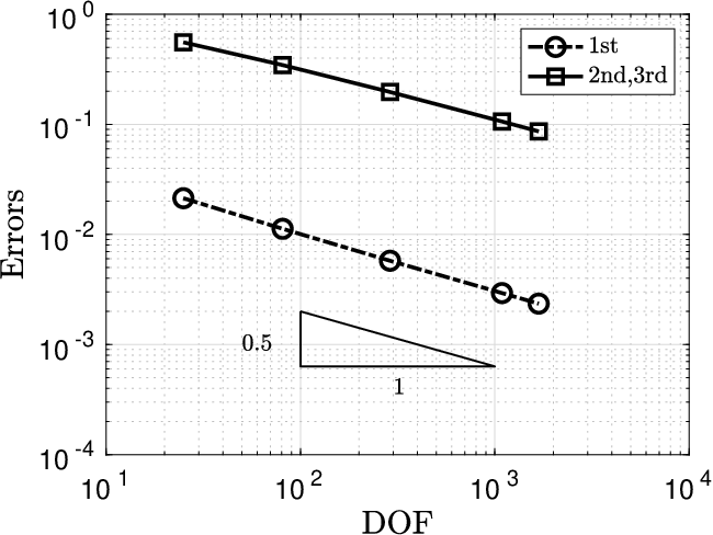
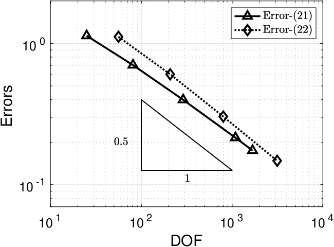
For the unit square domain, the eigenvalue estimations (5) for the leading eigenvalues are displayed in Tab. 3, while the results based on the nonconforming FEM ([50]) are displayed in Tab. 4. The results for the L-shaped domain are displayed in Tab. 5 and 6. Fig. 5 and Fig. 6 describe the relation between the absolute errors and the degrees of freedom (DOF) over the unit square and L-shaped domains, respectively. Here, the DOF of (5) is counted as the the dimension of the linear conforming FEM space , while the one for [50] is the dimension of the Crouzeix-Raviart FEM space.
Let us also introduce the total errors by
| Error-(23) |
The relation between the total errors and the degrees of freedom is displayed in Fig. 7.
Different from the nonconforming FEM in [50] which merely provide the guaranteed lower eigenvalue bounds, the conforming FEM produces both the upper bounds and the lower bounds of the eigenvalues. From the computational results for two domains and the comparison between the bound (5) and the one from [50], we draw the conclusion that
- (1)
Both the lower eigenvalue bounds proposed in this paper and the one in [50] have a sub-optimal convergence rate for the leading Steklov eigenvalues, compared with the convergence rate estimated by the numerical results themselves.
- (2)
| 0.2891 | 0.2042 | 0.1443 | 0.1021 | 0.51 | |
| 0.5740 | 0.4059 | 0.2870 | 0.2029 | 0.50 | |
| 0.6427 | 0.4544 | 0.3208 | 0.2272 | 0.51 | |
| 0.2404841 | 0.2401798 | 0.2401042 | 0.2400854 | 2.01 | |
| 0.218753 | 0.228833 | 0.2343144 | 0.2371468 | 0.95 | |
| 1.527151 | 1.502305 | 1.494918 | 1.492966 | 1.92 | |
| 0.936415 | 1.146662 | 1.295596 | 1.386153 | 0.72 |
(Note: , )
| 0.6110176 | 0.4038323 | 0.2714162 | 0.1848489 | 0.61 | |
|---|---|---|---|---|---|
| 0.2404829 | 0.2401793 | 0.2401041 | 0.2400853 | 2.0 | |
| 0.2206705 | 0.2311264 | 0.235931 | 0.2381318 | 1.13 | |
| 1.460229 | 1.483297 | 1.489892 | 1.491678 | 1.88 | |
| 0.9450309 | 1.19438 | 1.342541 | 1.419335 | 0.95 |
(Note: , )

| 0.5106 | 0.3633 | 0.2591 | 0.1847 | 0.48 | |
| 0.8118 | 0.5740 | 0.4059 | 0.2870 | 0.50 | |
| 0.9590 | 0.6793 | 0.4815 | 0.3413 | 0.50 | |
| 0.3443305 | 0.3421498 | 0.3416010 | 0.3414626 | 2.06 | |
| 0.2615119 | 0.2954914 | 0.3165279 | 0.3283997 | 0.93 | |
| 0.6513041 | 0.6299816 | 0.6217140 | 0.6186763 | 1.45 | |
| 0.4073133 | 0.4880800 | 0.5433766 | 0.5770854 | 0.89 | |
| 1.0278736 | 0.9968693 | 0.9876317 | 0.9851393 | 2.02 | |
| 0.5283698 | 0.6827630 | 0.8035932 | 0.8837230 | 0.85 |
| 0.8997886 | 0.5890361 | 0.3928155 | 0.2659045 | 0.63 | |
|---|---|---|---|---|---|
| 0.3425959 | 0.3416846 | 0.3414799 | 0.3414316 | 2.08 | |
| 0.2682036 | 0.3054704 | 0.3243874 | 0.3333834 | 1.07 | |
| 0.5829704 | 0.6039094 | 0.6120116 | 0.6150436 | 1.42 | |
| 0.3960439 | 0.4992908 | 0.5592028 | 0.5894119 | 0.99 | |
| 0.9608929 | 0.9769290 | 0.9821661 | 0.9837098 | 1.76 | |
| 0.5404476 | 0.7296185 | 0.8529063 | 0.9197389 | 0.88 |



4.4 Comparison with the optimal and proposed bound in (14)
In this subsection, we estimate the trace constant over several triangle ’s directly, and compare with its bound in (14). For , denote the th edge of by . Let us introduce the function space after in Lemma 2.
The trace constant is the quantity that makes certain the following estimation holds.
The determination of reduces to finding the minimal positive eigenvalue of the following Steklov eigenvalue problem:
| (24) |
By taking , the weak formulation of (24) is given as follows:
The strict lower eigenvalue bound for the above eigenvalue problem can be obtained by an analogous argument as performed in this paper, the detail of which is omitted here.
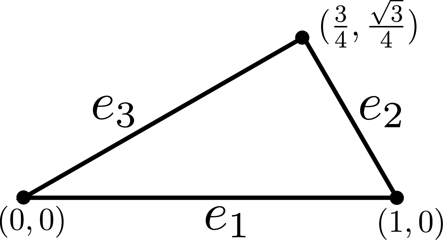
We consider three types of triangles (see Fig. 8) and evaluate by solving the corresponding Steklov eigenvalue problems using the linear conforming FEM. The results are shown in Tab. 7. It is observed that the bound in (14) is not too rough and a direct estimation of by solving the Steklov eigenvalue problem can obtain a sharper bound for the constant.


| Approximation of | Upper bound of | Upper bound in (14) | |||||||
|---|---|---|---|---|---|---|---|---|---|
| 0.7071 | 0.5516 | 0.5516 | 0.7198 | 0.5571 | 0.5571 | 1.1481 | 0.9654 | 0.9654 | |
| 0.6361 | 0.6361 | 0.6361 | 0.6446 | 0.6446 | 0.6446 | 0.8723 | 0.8723 | 0.8723 | |
| 0.7700 | 0.4285 | 0.7071 | 0.7843 | 0.4320 | 0.7169 | 1.2337 | 0.8723 | 1.1480 | |
5 Conclusion
In this paper, we propose a method to obtain the guaranteed lower bound of the Steklov eigenvalue by using the conforming FEM, where the hypercircle method plays an important role in obtaining the a priori error estimation. The proposed eigenvalue bounds have a degenerated convergence rate as , when the FEM approximations of the leading eigenvalues demonstrate the convergence rate. Such a degenerated convergence rate of our propose method cannot be improved, because the involved projection error estimate has to handle the worst case when the solution to boundary value problem does not have the regularity. In future work, the authors will apply the Lehmann–Goerisch’s theorem to obtain lower eigenvalue bounds with optimal convergence rates.
Funding: The first author is supported by JST SPRING, Grant Number JPMJSP2121. The second author has been supported by the National Natural Science Foundation of China (No.11426039,12061057,11571023). The last author is supported by Japan Society for the Promotion of Science: Fund for the Promotion of Joint International Research (Fostering Joint International Research (A)) 20KK0306, Grant-in-Aid for Scientific Research (B) 20H01820, 21H00998. This work also received support from the Research Institute for Mathematical Sciences, an International Joint Usage/Research Center located in Kyoto University.
References
- [1] M. Ainsworth and T. Vejchodský, Robust error bounds for finite element approximation of reaction–diffusion problems with non-constant reaction coefficient in arbitrary space dimension, Comput. Methods Appl. Mech. Eng., 281 (2014), pp. 184–199.
- [2] M.G. Armentano and C. Padra, A posteriori error estimates for the Steklov eigenvalue problem, Appl. Numer. Math., 58 (2008), no. 5, pp. 593–601.
- [3] I. Babuška and J. Osborn, Eigenvalue Problems, Finite Element Methods (Part 1), Handbook of Numerical Analysis, Vol. II, Elsevier Science Publishers B.V., North-Holland, 1991.
- [4] S. Bergman and M. Schiffer, Kernel functions and elliptic differential equations in mathematical physics, Academic Press, New York, 1953.
- [5] A. Bermúdez, R. Rodríguez, and D. Santamarina, A finite element solution of an added mass formulation for coupled fluid-solid vibrations, Numer. Math., 87 (2000), no. 2, pp. 201–227.
- [6] H. Bi, Y. Zhang, and Y. Yang, Two-grid discretizations and a local finite element scheme for a non-selfadjoint Stekloff eigenvalue problem, Comput. Math. Appl., (2018).
- [7] G. Birkhoff, C. De Boor, B. Swartz, and B. Wendroff, Rayleigh-Ritz approximation by piecewise cubic polynomials, SIAM J. Numer. Anal., 3 (1966), no. 2, pp. 188–203.
- [8] D. Boffi, Finite element approximation of eigenvalue problems, Acta Numer., 19 (2010), pp. 1–120.
- [9] J.H. Bramble and J. Osborn, Approximation of Steklov eigenvalues of non-selfadjoint second order elliptic operators, The mathematical foundations of the finite element method with applications to partial differential equations, Elsevier, 1972, pp. 387–408.
- [10] F. Brezzi and M. Fortin, Mixed and Hybrid Finite Element Methods, Springer Series in Computational Mathematics, vol. 15, Springer, 1991.
- [11] F. Cakoni, D. Colton, S. Meng, and P. Monk, Stekloff eigenvalues in inverse scattering, SIAM J. Appl. Math., 76 (2016), no. 4, pp. 1737–1763.
- [12] E. Cancès, G. Dusson, Y. Maday, B. Stamm, and M. Vohralík, Guaranteed and robust a posteriori bounds for Laplace eigenvalues and eigenvectors: conforming approximations, SIAM J. Numer. Anal., 55 (2017), no. 5, pp. 2228–2254.
- [13] , Guaranteed and robust a posteriori bounds for Laplace eigenvalues and eigenvectors: a unified framework, Numer. Math., 140 (2018), no. 4, pp. 1033–1079.
- [14] , Guaranteed a posteriori bounds for eigenvalues and eigenvectors: Multiplicities and clusters, Math. Comp., 89 (2020), no. 326, pp. 2563–2611.
- [15] C. Carstensen, A. Ern, and S. Puttkammer, Guaranteed lower bounds on eigenvalues of elliptic operators with a hybrid high-order method, Numer. Math, 149 (2021), no. 2, pp. 273–304.
- [16] C. Carstensen and D. Gallistl, Guaranteed lower eigenvalue bounds for the biharmonic equation, Numer. Math., 126 (2014), no. 1, pp. 33–51.
- [17] C. Carstensen and J. Gedicke, Guaranteed lower bounds for eigenvalues, Math. Comput., 83 (2014), no. 290, pp. 2605–2629.
- [18] C. Carstensen and S. Puttkammer, Direct guaranteed lower eigenvalue bounds with optimal a priori convergence rates for the bi-Laplacian, arXiv preprint arXiv:2105.01505, (2021).
- [19] C. Carstensen, Q. Zhai, and R. Zhang, A skeletal finite element method can compute lower eigenvalue bounds, SIAM J. Numer. Anal., 58 (2020), no. 1, pp. 109–124.
- [20] F. Demengel, G. Demengel, and translated by R. Erné, Functional spaces for the theory of elliptic partial differential equations, Springer, 2012.
- [21] D. Gallistl and V. Olkhovskiy, Computational lower bounds of the Maxwell eigenvalues, arXiv preprint arXiv:2110.02605, (2021).
- [22] J.L. Guermond and A. Ern, Finite Elements II: Galerkin Approximation, Elliptic and Mixed PDEs, Springer, 2021.
- [23] J. Hu, Y. Huang, and Q. Lin, Lower bounds for eigenvalues of elliptic operators: by nonconforming finite element methods, J. Sci. Comput., 61 (2014), no. 1, pp. 196–221.
- [24] J. Hu, Y. Huang, and R. Ma, Guaranteed lower bounds for eigenvalues of elliptic operators, J. Sci. Comput., 67 (2016), no. 3, pp. 1181–1197.
- [25] F. Kikuchi and X. Liu, Estimation of interpolation error constants for the P0 and P1 triangular finite elements, Comput. Method Appl. M., 196 (2007), no. 37-40, pp. 3750–3758.
- [26] K. Kobayashi, On the interpolation constants over triangular elements (in Japanese), Kyoto University Research Information Repository, 1733 (2011), pp. 58–77.
- [27] K. Kobayashi, On the interpolation constants over triangular elements, Appl. Math., (2015), pp. 110–124.
- [28] N. Kuznetsov, T. Kulczycki, M. Kwaśnicki, A. Nazarov, S. Poborchi, I. Polterovich, and B. Siudeja, The legacy of Vladimir Andreevich Steklov, Notices of the AMS, 61 (2014), no. 1, pp. 190.
- [29] M. Li, Q. Lin, and S. Zhang, Extrapolation and superconvergence of the Steklov eigenvalue problem, Adv. Comput. Math., 33 (2010), no. 1, pp. 25–44.
- [30] Q. Li, Q. Lin, and H. Xie, Nonconforming finite element approximations of the Steklov eigenvalue problem and its lower bound approximations, Appl. Math., 58 (2013), no. 2, pp. 129–151.
- [31] Q. Li and X. Liu, Explicit finite element error estimates for nonhomogeneous Neumann problems, Appl. Math., 63 (2018), no. 3, pp. 367–379.
- [32] Q. Li and Y. Yang, A two-grid discretization scheme for the Steklov eigenvalue problem, J. Appl. Math. Comput., 36 (2011), no. 1-2, pp. 129–139.
- [33] S. Liao, Y. Shu, and X. Liu, Optimal estimation for the Fujino–Morley interpolation error constants, Jpn. J. Ind. Appl. Math., 36 (2019), no. 2, pp. 521–542.
- [34] Q. Lin, H. Xie, F. Luo, Y. Li, and Y. Yang, Stokes eigenvalue approximations from below with nonconforming mixed finite element methods, Math. Pract. Theory, 40 (2010), no. 19, pp. 157–168.
- [35] J. Liu, J. Sun, and T. Turner, Spectral indicator method for a non-selfadjoint Steklov eigenvalue problem, J. Sci. Comput., 79 (2019), no. 3, pp. 1814–1831.
- [36] X. Liu and S. Oishi, Verified eigenvalue evaluation for Laplace operator on arbitrary polygonal domain max and max-min principle, RIMS Kokyuroku, 1733 (2011), pp. 31–39.
- [37] X. Liu, A framework of verified eigenvalue bounds for self-adjoint differential operators, Appl. Math. Comput., 267 (2015), pp. 341–355.
- [38] X. Liu and S. Oishi, Verified eigenvalue evaluation for the Laplacian over polygonal domains of arbitrary shape, SIAM J. Numer. Anal., 51 (2013), no. 3, pp. 1634–1654.
- [39] X. Liu and C. You, Explicit bound for quadratic Lagrange interpolation constant on triangular finite elements, Appl. Math. Comput., 319 (2018), pp. 693–701.
- [40] M.T. Nakao, M. Plum, and Y. Watanabe, Numerical verification methods and computer-assisted proofs for partial differential equations, Springer, 2019.
- [41] A.D. Russo and A.E. Alonso, A posteriori error estimates for nonconforming approximations of Steklov eigenvalue problems, Comput. Math. Appl., 62 (2011), no. 11, pp. 4100–4117.
- [42] G. Savaré, Regularity results for elliptic equations in Lipschitz domains, J. Funct. Anal., 152 (1998), no. 1, pp. 176–201.
- [43] I. Sebestová and T. Vejchodský, Two-sided bounds for eigenvalues of differential operators with Applications to Friedrichs, Poincaré, trace, and similar constants, SIAM J. Numer. Anal., 52 (2014), no. 1, pp. 308–329.
- [44] J. Sun and A. Zhou, Finite element methods for eigenvalue problems, Chapman and Hall/CRC, 2016.
- [45] H. Xie, A type of multilevel method for the Steklov eigenvalue problem, IMA J. Numer. Anal., 34 (2014), no. 2, pp. 592–608.
- [46] H. Xie, M. Xie, X. Yin, and M. Yue, Computable error estimates for a nonsymmetric eigenvalue problem, East Asian J. Appl. Math., 7 (2017), no. 3, pp. 583–602.
- [47] M. Xie, H. Xie, and X. Liu, Explicit lower bounds for Stokes eigenvalue problems by using nonconforming finite elements, Japan J. Indust. Appl. Math., 35 (2018), no. 1, pp. 335–354.
- [48] Y. Yang, Q. Li, and S. Li, Nonconforming finite element approximations of the Steklov eigenvalue problem, Appl. Numer. Math., 59 (2009), no. 10, pp. 2388–2401.
- [49] Y. Yang, Z. Zhang, and F. Lin, Eigenvalue approximation from below using non-conforming finite elements, Sci. China Math., 53 (2010), no. 1, pp. 137–150.
- [50] C. You, H. Xie, and X. Liu, Guaranteed eigenvalue bounds for the Steklov eigenvalue problem, SIAM J. Numer. Anal., 57 (2019), no. 3, pp. 1395–1410.
- [51] Y. Zhang, H. Bi, and Y. Yang, Asymptotic lower bounds for eigenvalues of the Steklov eigenvalue problem with variable coefficients, Appl. Math., 66 (2021), no. 1, pp. 1–19.
- [52] Y. Zhang and Y. Yang, Guaranteed lower eigenvalue bounds for two spectral problems arising in fluid mechanics, Comput. Math. Appl., 90 (2021), pp. 66–72.