Crossing the phantom divide line as an effect of quantum transitions
Abstract
We consider the Chiral cosmological model consisting of two scalar fields minimally coupled to gravity. In the context of a Friedmann–Lemaître–Robertson–Walker (FLRW) spacetime, and for massless fields in the presence of a cosmological constant, we present the general solution of the field equations. The minisuperspace configuration that possesses maximal symmetry leads to scenarios which - depending on the admissible value of the parameters - correspond to a quintessence, quintom or phantom case. The canonical quantization of the model retrieves this distinction as different families of quantum states. The crossing of the phantom line is related to the existence of free or bound states for the Casimir operator of the symmetry algebra of the fields. The classical singularity, which is present in the quintessence solution, is also resolved at the quantum level.
Keywords:
Scalar field; cosmology; exact solutions; quantum cosmologyAugust 11, 2026
I Introduction
Scalar fields play an important role in cosmological studies because they provide processes with the means to explain the recent cosmological observations Teg; Kowal; Komatsu; planck; planck18. Specifically, the obtained cosmological data indicate that our universe has gone through two acceleration phases in its evolutionary history. The late accelerated expansion, which appears to continue until today, and an early acceleration phase known as inflation.
In order to expain the observed isotropization of the universe at large scales it has been suggested that the universe has gone through an expansion era known as inflation. The main theoretical mechanism which has been proposed to describe the inflationary era is based on the existence of a scalar field known as the inflaton guth. The latter dominates for a short period the dynamics which drive the evolution of the universe so that, at large scales, it appears to be isotropic and homogeneous.
For the recent acceleration era of the universe, scalar fields can also assume the role of the dark energy Ratra; BarrowSF. To this end, cosmologists consider a contribution in the Einstein field equations with the property that the resulting effective fluid has an equation of state parameter . The pure cosmological constant model is the simplest dark energy model in terms of dynamics and its behaviour. The corresponding equation of state parameter for the fluid source described by the cosmological constant is and does not vary during the evolution of the universe. However, because of its simplicity in terms of dynamics, the cosmological constant cannot explain the complete cosmological history and suffers from two major drawbacks, known as the fine tuning and the coincidence problem Weinberg1; Padmanabhan1. Consequently, the models proposed by cosmologists to overpass these difficulties, made the scalar field important in the study of the cosmological evolution.
Recently in bavacu, the authors used a classical scalar field, called the “vacuumon”, in the description of running vacuum models. It was demonstrated that the scalar field description is very helpful for the explanation of the physical mechanisms of the running vacuum models during both the early universe and the late time cosmic acceleration bavacu. This was not the first attempt where scalar fields were used for the depiction of various dark energy models: In sol1v a scalar field configuration was used as a representative model for the description of a running vacuum theory. The scalar field representation of a matter creation model was presented in spn1, while a realization of the generalized Chaplygin gas was given in cg1; we refer the reader in inf1 and references therein for a scalar field description of the modified Chaplygin gas.
Furthermore, scalar fields can be used as new degrees of freedom to obtain analogous results to those obtained from modified theories of gravity, which generalize Einstein’s theory of General Relativity bd; fr1; fr2; fr3; ft1; ft2; fg1; fg2; Oik. Indeed, the supergravity inflationary model aastar, known as Starobinsky inflation can be described by a scalar field, where the potential of the inflaton is constructed by the supergravity model by using a Lagrange multiplier and a conformal transformation oo0; a standard approach which relates the Jordan and the Einstein frames of scalar field models oo1; oo2; oo3; oo4.
Quintessence is the simplest scalar field proposed by Ratra et al. Ratra. The energy density of the scalar field is always positive while the parameter for the equation of state, namely , is bounded as . In the limit , only the kinetic part of the scalar field contributes in the evolution of the universe. On the other hand, when , the scalar field mimics the cosmological constant. One of the main characteristics of the quintessence is the unstable tracker solution, for more details on the dynamics of the quintessence we refer the reader in qui1; qui2; qui3; qui4; qui5; qui6; qui7.
The cosmological observations does not provide a lower limit for the value of . While it has a value close to , the values in the range are not excluded by the cosmological observations ph1; ph2; ph3; ph4; ph5; ph6. Hence, scalar fields with phantom kinetic energy have been introduced in the literature sph1; sph2. The phantom cosmological models generally lead to a big rip, however - as it has been shown by various studies - this can be overpassed, for details see br01; br02; br03; br04.
It has been proposed that the equation of state parameter may have crossed the phantom divide line more than once, leading to the quintom scalar field cosmology qq1; qq2; qq3. The latter theory consists of two-scalar fields (one quintessence and one phantom) which interact, not necessarily in the potential term. In quintom cosmology, the second scalar field introduces new degrees of freedom, which provide more possibilities towards the cosmological evolution. Therefore, multi-scalar field models have been introduced by cosmologists for the description of the various eras of the universe mmf1; mmf2; mmf4.
In this work, we are interested in a two-scalar field cosmology known as Chiral cosmology chir3. In this gravitational theory, the two scalar fields are minimally coupled to gravity; however they are necessarily interacting in the kinetic part. This cosmological model is related to the non-linear sigma cosmological model sigm0; sigm1. This specific theory is also linked to the attractor model which has been used as an alternative for the description of inflation and also as a dark energy model al1; al2; al3; al4; al5; al6; all7; al8.
For the latter gravitational theory and for a homogeneous Friedmann–Lemaître–Robertson–Walker (FLRW) spacetime we present a set of analytic solutions which can describe the phantom and the quintessence epochs of the universe. Additionally, we demonstrate how these two distinct cosmological solutions correspond to different sets of quantum states. Thus, making the passing of the phantom divide line a matter of quantum transitions (e.g. bound to free states).
Specifically, because the gravitational theory of our consideration admits a minisuperspace description, we apply the canonical quantization which leads to the Wheeler-DeWitt equation DeWitt. At the quantum level we define, from the classical conservation laws of the field equations, quantum operators which are used as supplementary conditions over the Wheeler-DeWitt equation. This approach has been applied before and has lead to various interesting results in cosmological and gravitational models qu2; qu3; Pailas where it can be seen that in the semiclassical limit the curvature singularities can be avoided qu4. The novelty of this approach is that quantum observables and their eigenvalues can be related to classical constants of integration appearing in the metric qu5; qu6; qu7. In this work, we see that the Chiral cosmology, which classically may lead to either quintessence or a phantom field(s), at the quantum level brings about different sets of eigenvalues depending on the classical equivalent of the system. Thus connecting different quantum states to distinct classical behaviours.
In Section II, we present the cosmological model of our consideration which is that of Chiral cosmology in a FLRW spacetime. For the scalar field potential we consider the simplest case, which requires the latter to be constant, such that only the kinetic part of the scalar fields is a time-varying function. In other words, we assume the two scalar fields to be massless. We calculate the conservation laws of the field equation which are generated by the elements of the Lie algebra. The classical solution of the field equations for the cases with or without spatial curvature is presented in Section III. For the spatially flat spacetime and for a specific value of one of the free parameters of the model we are able to write the analytic solution in closed form functions. We observe that for different values of the integration constants we are able to recover distinct solutions which we call quintessence () or phantom () epochs.
The quantization method that is followed is presented in Section IV. We calculate the wave function of the universe for the generic model of our consideration. In Section V we present, for the specific values of the parameters examined at the classical level, an extended analysis where we show how the two different classical behaviours, i.e. the quintessence and the phantom epochs, are represented by different families of quantum states. Finally, our discussion on the results in given in Section VI and in the appendices some mathematical calculations which are necessary for our analysis are presented.
II The cosmological model
We consider two massless scalar fields minimally coupled to Einstein’s gravity in the presence of a cosmological constant
| (1) |
with the two scalar fields, and , interacting in the kinetic part. The two-dimensional space, which is defined by the kinetic term of the scalar fields, is a space of constant curvature. Such an Action Integral is invariant under the group Maharana1; Maharana2; Cordero. The appearing in (1) is a nonzero free parameter associated to the scalar constant curvature of the two-dimensional field space.
Variation of the Action Integral (1) with respect to the metric tensor and the scalar fields leads to the gravitational field equations which are:
| (2) | ||||
| (3) | ||||
| (4) |
where , are the Ricci scalar and tensor corresponding to the spacetime metric . Moreover, the energy momentum tensor consisted by the two scalar fields is given by the following formula:
| (5) |
We assume that the spacetime is described by the FLRW line element
| (6) |
where denotes the spatial curvature. Unless we want the fields and to have mutually cancelling contributions in (1), leading to , we need to set (for the consistency of Einstein’s equations) and .
By freezing out the spatial coordinates in the original action (1) we are led to a minisuperspace Lagrangian which reads
| (7) |
The Euler-Lagrange equations are generated by varying Lagrangian (7) with respect to the kinematic quantities , and can be expressed as
| (8) |
| (9) | ||||
| (10) | ||||
| (11) |
these are completely equivalent to the reduced system which is obtained from the field equations (2)-(4), under the ansatz (6) for the spacetime and a pure time dependence of the fields.
Due to invariance of the action under the group, the system admits the point symmetries with generators
| (12) |
which can be used to construct conservation laws for the field equations by using the method of variational symmetries. For example, we observe that from equation (4) we get the conserved quantity
| (13) |
which is generated by the symmetry vector field .
III Classical solution
For the convenience of our analysis, we perform a reparametrization of the lapse : that leads to the equivalent point-like Lagrangian for the field equations
| (14) |
where . In the case of a spatially flat spacetime , Lagrangian describes the motion of a free relativistic particle of mass in the minisuperspace of characterized by the metric which reads
| (15) |
The corresponding Ricci scalar of the minisuperspace is calculated to be
| (16) |
The three , , of (12) are Killing vectors of . For the particular values the minisuperspace metric describes a three dimensional flat space and admits three additional Killing vectors. This case is the one which is going to be of most interest in our analysis. Let us begin however with some general remarks regarding the generic situation.
The three Killing vectors of - since they also leave invariant the potential term of (14) - define integrals of motion of the form
| (17) |
where are the momenta associated with the velocities and .
By utilizing the three equations , where are constants; it is easy to obtain
| (18) | ||||
| (19) |
where we reparametrized the constants and in terms of the new parameters .
Substitution of the above expressions into the equations of motion (8)-(11) leaves us only to solve the constraint (8), which reduces to
| (20) |
The previous equation can be easily integrated to give in terms of . The latter remains an arbitrary function due to the fact that we did not adopt some specific time gauge for the system. The resulting expression is quite complicated and given in terms of an elliptic integral of the third type, which we refrain from giving here. Nevertheless, in the particular cases where , and the solution can be written in terms of elementary functions:
(II) The case leads to
| (22) |
where is the constant of integration.
(III) Finally, when the resulting expression for the scale factor is
| (23) |
where the constant is introduced and is again the integration constant.
III.1 The spatially flat universe with
We mentioned that, for the spatially flat universe, i.e. , and when , the resulting Lagrangian (14) describes a free relativistic particle moving in a three dimensional flat space. Thus, for these values of the parameters the system admits three additional linear in the momenta integrals of motion11 1 The generators of the three additional conserved charges are those of the typical translations, when the minisuperspace is in coordinates where . on top of the conserved charges (17) which are produced by the group whose generators are given by (12). In this sense it is a system of maximal symmetry in what regards the minisuperspace description.
Depending on the admissible values of the parameters involved in the solution, various gravitational behaviours can be obtained. It is possible to reparametrize the constants of integration so that the solution reads (for the detailed derivation please see the appendix A)
| (24) |
| (25) |
| (26) |
where we have chosen the time gauge in which essentially the field becomes the time variable.
Note that the above form of solution is minimal in the sense that we have eradicated integration constants that can be absorbed by means of reparametrizations and diffeomorphisms (for details see appendix A). The constant in (24) is of course absorbable by a constant scaling in the variable in the metric (6). However we choose to keep it because it can serve to maintain real under different choices for the rest of the parameters.
Expressions (24)-(26) satisfy the field equations (9)-(11), while the constraint equation (8) yields the following relation among constants
| (27) |
As we may observe from (24)-(26), the solution is periodic and the region of for which you can have real and depends on the free parameters of the solution. We note that the parameters involved in (24) and (25) may assume any value as long as the end result has some real domain of definition. For example, it can be easily seen, that we can set and to be simultaneously imaginary and have both (24) and (25) as real functions for some interval of . In the following section we treat separately two distinct cases which give interesting behaviours that are related with the rate of the expansion of the universe.
III.2 The quintessence epoch
Here we study the solution (24)-(26) when the related parameters assume such values, so that it describes a universe whose equation of state parameter, , of the relevant effective fluid ranges from to . Thus, characterizing what we shall refer to as a “quintessence epoch”. The and are the energy density and the pressure of the effective cosmological perfect fluid that produces the same energy-momentum tensor as the of (5).
Let us study the functional behaviour of the solution assuming , and , while are both real.22 2 The range of values of and have been assumed in this manner so that we obtain an expansive behaviour for the scale factor. In order for the latter to be true - and given the restriction we set on - we need to have . Under these conditions and assuming , (24) and (25) are real in the interval . A behaviour that is being repeated with a period of .
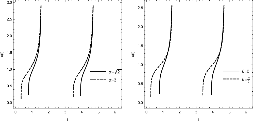
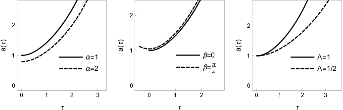
In figure 1 we demonstrate how the scale factor is affected by different values of the parameters and . In order to obtain a more physical insight of the solution we need to express the result in terms of the cosmological (or cosmic) time in which . Thus, we introduce a new time variable given by
| (28) |
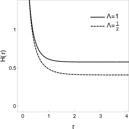
The application of its inverse however in the analytic solution of the problem, cannot in general result in expressions given in terms of elementary functions. Nevertheless, we are able, in figures 2 and 3 to give some parametric plots for the scale factor and the Hubble function as functions of the cosmological time defined by (28). We need to note that in the plots, the choice of the values of the parameters is made so as to demonstrate in a simple manner how they affect the behaviour of the functions, it is not with reference to observational values.
As we see in figure 2 the values of and affect the “steepness” of the expansion in an opposite manner. Larger values of lead to a milder expansion, while in what regards this happens for smaller values. On the other hand just translates the graph in time, which is unimportant if you consider that transformation (28) already has the freedom of adding an arbitrary constant and thus shifting in time the whole graph. In figure 3 we see how the Hubble parameter is affected by , which dominates the value towards which asymptotically tends. Recall that in the time gauge of (24) and (25) the Hubble function is given by .
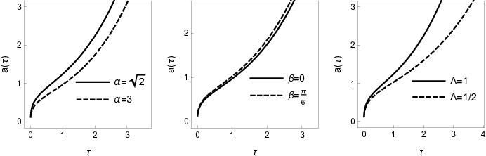
It is interesting to note that the finite region corresponds through the inverse of (28) to a cosmological time . What it is more, the limit (or equivalently in cosmological time) corresponds to a curvature singularity for the spacetime whose metric is characterized by (24) and (25).
The effective fluid energy density and pressure that we can read from the energy momentum tensor (5) are
| (29) |
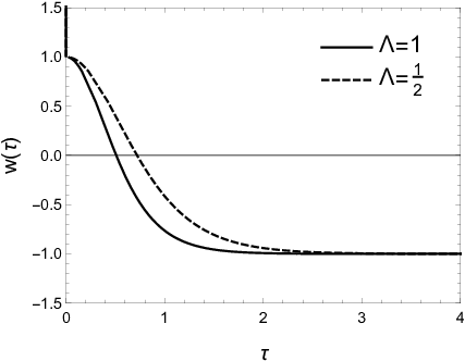
In the particular case that we study, where and the analytical solution is given by (24) under the constraint (27), we calculate the equation of state function to be
| (30) |
From (30) we observe that for , that is, only the cosmological constant contributes in the universe in this limit. However, the latter is not true near the cosmological singularity, i.e. . In this case . We remark that for the general solution reduces exactly to that of the de Sitter universe.
Although does not depend on , when the function is expressed in terms of the cosmological time , the corresponding does. Because the transformation (28), through (25) and (27) involves in the process. In this manner we are able to plot what we see in figure 4.
III.3 The phantom epoch ()
As we previously observed, the gravitational part of the solution remains real if we take and to be imaginary. We thus start by assuming, and , where . With the help of this substitution, the analytic solution (24)-(26) can be brought to the form
| (31) | ||||
| (32) | ||||
| (33) |
with the constraint (27) among the constants becoming
| (34) |
We observe that this parameterization results in an imaginary field , which - by looking at the action (1) - signifies that both and become phantom fields. Of course, we expect that this allows to cross the phantom divide line and to take values smaller than . Because of the latter property, we call that era “phantom epoch”.
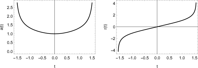
Let us assume once more a phase . Then, and as given by (31), (32) are real in the region , assuming , with the same behaviour being repeated with a period of . In figure 5 we present the plot of the scale factor as function of the cosmological time defined by (28). We observe that at the origin, , the scale factor obtains a finite non-zero value. It is also easy to verify, by looking at the Ricci and Kretschmann scalars, and respectively, that the spacetime characterized by (31) and (32) has no curvature singularity. For example, by using (31), (32) and (34), the Ricci scalar becomes
| (35) |
which is finite for the values of the parameters considered, i.e. . The numerator consists of trigonometric functions which are bounded, while the denominator cannot be zero. The same is true for the Kretschmann scalar, whose expression however is quite more complicated and which we avoid to present here. We see thus that in this case no curvature singularity occurs and, as we demonstrate below, a bounce solution is obtained.
In order to expose the bouncing solution we need to write an extension of what we see in Fig. 5 for times before . Due to the arbitrariness of a multiplicative constant in and because is invariant in an overall sign (see eqs. (31) and (32) respectively) we can construct a smooth extension of the solution for . In order to do so we require to have a real expression for the scale factor throughout the region . The latter is achieved by the function
| (36) |
In other words we take to be constituted of two branches: For we consider (31) with , while for we use the same relation but with (remember that we consider ). Note that expression (36) for the scale factor is continuous at the limit and the same is true for its derivatives with respect to . The latter does not hold for the expresion without the absolute value. In a similar fashion we need to construct a smooth expression for . The arbitrariness of the overall sign in (32) is enough for that matter, hence we take
| (37) |
The cosmological time which is related to through (28) is calculated to be
| (38) |
For this function, the zero of the cosmological time, , is placed at
| (39) |
which is also the time for which the of (36) assumes its minimum value. It is an easy task to verify that and . As an illustrative example, in Fig. 6, we plot the functions (36) and (38) for some specific values of the parameters.
As far as the scalar fields are concerned regarding the continuity: It is straightforward that of (33) is continuous since it is effectively the time parameter itself. For in (33) a similar process as for the can be followed due to the arbitrariness of the solution in the sign. We can thus take
| (40) |
which makes the a continuous function throughout . We notice that the calculated from (40) possesses a discontinuity in . Specifically we obtain, while on the other hand we have . However, this creates no particular problem since what enters the Lagrangian and the physically relevant quantities, like the effective energy density and the pressure is the which is continuous in all its domain of definition. The aforementioned discontinuity in defined by (40) is present in all odd derivatives of , the even derivatives like remain continuous.
From the moment that the scale factor does not become zero and stays positive we know that non-spacelike geodesics are past-complete Lam. Thus, unlike to what we obtain in the quintessence case, where such a construction is not possible, here the spacetime has no initial singularity and describes a bouncing universe. We also note that there is no big rip in the future since the scale factor does not go to infinity in some finite time . It is for that .
In what regards the description of the effective perfect fluid and the equation of state parameter , we can straightforwardly set in (30) to obtain
| (41) |
which obviously is lesser that for all values of . At the limit , the parameter assumes its maximum value .
An important remark is that a similar behaviour of expansion for can be obtained by assuming only to be imaginary, while . In order to keep real the solution expressed by (31) we need to set . The plus or minus in the exponent depends on the branch we need to consider, or respectively. We can thus state, that needs to be imaginary; from there we have two paths that we may follow depending on the possible values we may assign to and .
It is quite interesting to observe that in the case where we take only to be imaginary, the result is obtained with just one of the two fields turning phantom, namely the . The becomes complex, but with a constant imaginary part of . As a result its derivative is real and the corresponding kinetic term in (1) does not change sign. On the other hand, the in front of becomes negative since , which explains how the line is crossed.
III.4 The de Sitter limit
Until now we studied the behaviour of the classical solution for the field equations of the model with Action Integral (1). We found that there can be an exact solution which describes a quintessence era and another solution which describes a bounced universe with at least one phantom field. While the two models are distinct and they have different analytic solutions and behaviour, it is important to mention that the two different solutions have as an attractor the de Sitter universe with . However, they reach the attractor from different directions. In the case of the quintessence, decreases and reach the value , while in the case of the phantom field, increases and the value plays the role of an upper wall. This can be seen from equations (30) and (41). The limit is the asymptotic future of the spacetimes since in the cosmic time gauge, i.e. when , it corresponds to . In that limit both (30) and (41) tend to the value . In the first case the limit is reached from values , while in the latter from .
Another way to observe the same effect is through the energy momentum tensor. A simple substitution of either (24)-(26) or (31)-(33) leads to all the components of the mixed tensor to be proportional to . As a result, the limit leads to and the cosmological constant in (2) to dominate the future of both spacetimes. The de Sitter solution becomes the asymptotic future in both cases.
Similarly, at the level of the metric, we may consider an expansion of either solution (24), (25) or (31), (32) when . In both of these cases the leading terms in the expansion around are
| (42) |
where the relations (27) and (34) have also been applied in each of the corresponding solution. With the help of the transformation (28) we see that is related to through
| (43) |
We write the resulting approximate line element at the limit (or equivalently at ) as
| (44) |
which is the de Sitter solution with cosmological constant . Note that in the above line element we ignored the multiplicative constant appearing in coming from (42) since it is absorbable with a diffeomorphism (in particular a constant scaling) in the radial distance .
Having studied the classical aspects of each case we may now proceed to the quantum description of the system. In the following section we shall see how we can pass from one solution to another through quantum processes. The analysis is performed under the scope of canonical quantum cosmology and the use of the Wheeler-DeWitt equation.
IV Quantization of the general model
The quantization of the system described by Lagrangian (14) is straightforward. We apply the Dirac-Bergmann Dirac; AndBer algorithm for constrained systems in order to pass to the Hamiltonian formulation. We sketch the basic steps here, but for more details we refer the interested reader to textbooks on constrained systems Dirac2; Sund.
The starting point is Lagrangian as seen in (14). Obviously there is no velocity for the degree of freedom , which makes the corresponding momenta to be zero and at the same time the Legendre transformation non-invertible. In such cases the Dirac-Bergmann algorithm is used to pass to the Hamiltonian description of the system. In our case is the primary constraint of the theory, with “’’ denoting a weak equality33 3 Having a quantity being weakly zero roughly signifies, that it is not to be set to zero prior to any Poisson bracket calculation. Only the end result is to be projected on the constrained surface where the constraints vanish. For example, means that , but , i.e. the zero value of cannot be substituted when the latter is inside a Poisson bracket.. The primary constraint is added in the Hamiltonian through a multiplier which is denoted here by . The can be seen as the missing velocity of . Thus, the total Hamiltonian is defined as
| (45) |
where the momenta are given by and is the inverse of the minisuperspace metric (15). The is called the quadratic (or Hamiltonian) constraint. It results as such due to the consistency requirement that any of the constraints must be (at least through a weak equality) preserved in time. Thus, for , we need to have , which leads to
| (46) |
Hence, becomes the secondary constraint of the theory. No tetriary constraint is derived since the consistency condition is satisfied identically. As a result our theory has two constraints, namely and . They additionally commute with each other , which categorizes them as first class constraints and signifies that the multiplier , as well as , in (45) remain arbitrary functions of the theory. The total Hamiltonian results in being a linear combination of constraints.
Since at this level we deal with a simple quantum mechanics problem, we follow the canonical quantization procedure. We thus choose the typical representation where the positions act multiplicatively while the momenta are first order linear operators (in what follows we work in units)
| (47) |
We put in use Dirac’s procedure for quantizing constrained systems and thus we require that the constraints impose the following conditions upon the wave function
| (48) | ||||
| (49) |
The first relation simply states that cannot depend on and the second defines the well known Wheeler-DeWitt equation.
In order to address the factor ordering problem of the Hamiltonian constraint operator, whose classical equivalent is (46), we choose the conformal Laplacian in order to express its kinetic term. The reason for this is twofold tczan: a) The wave functions that result as solutions of can give an invariant probability amplitude under transformations in the configuration space, where is the corresponding volume element and , with , the natural measure. b) The conformal Laplacian is invariant under conformal transformations of the minisuperspace metric ConfLap. The latter is compatible with the scaling the lapse function that we have used at the classical level. It is the freedom which we exploited in order to pass from to and to the minisuperspace metric (15). Hence we have
| (50) |
where is the Ricci scalar of the minisuperspace given in (16) and its dimension.
The two additional operators that we need in order to distinguish a complete set of states solving (48) are given by considering the quantization of the algebra. First we express the classical observables of (17) as operators. To this end we adopt the most general expression for a linear first order Hermitian operator under a measure
| (51) |
The fact that we use the physical measure , together with the being Killing vector fields of , reduces the generic expression (51) to just tchriSw. In our case the vectors are those presented in (12). By construction, the commute with the Hamiltonian constraint operator of (50).
In this setting the inner product between two states, which are characterized by the wavefunctions and , is given by
| (52) |
where we have substituted as the determinant of the minisupermetric (15). There is an overall numerical factor in the determinant which without loss of generality we can ignore. When we later construct the orthonormal states such a numerical factor can always be absorbed inside the normalization constant. Only the functional dependence of on the configuration space variables is effectively important. As we mentioned before, this choice of measure, together with the operators we adopted, results in the inner product being invariant under diffeomorphisms of the minisuperspace metric tczan. We thus carry a geometric property of the classical minisuperspace - the fact that the latter is invariant under diffeomorphisms - to the quantum level of the inner product and subsequently to the definition of the probability. In what follows below we perform various transformations in the variables depending on which offers in each case a better simplification of the results. With the adoption of the square root of the determinant of the minisuperspace metric as a measure we have guaranteed that this does not affect the quantization process.
In order to proceed with the quantization, we need to use , the Casimir invariant of the algebra and of course as a constraint on the wave function. We already know that the algebra - which is closely related to the Pöschl-Teller problem in quantum mechanics - results in states characterized by two eigenvalues , with
| (53) |
where the constant factor (the same appearing in the starting action (1)) has been introduced at the right hand side for simplification reasons. Alternatively - in what regards these two equations - we could also absorb it inside and .
The main difference with the typical angular momentum quantization of is that may also assume negative values. The significance of the algebra in the quantum cosmology of the axion - dilaton system, has already been observed in Maharana1; Maharana2; Cordero, where a specific coupling inspired by string theory is assumed in the field kinetic terms in the context of a positive spatial curvature FLRW spacetime without cosmological constant. The algebra quantization has also been connected with systems obtained in a minisuperspace procedure Dimakis1; Kara.
We start from the general case and present the solutions that we derive, but restrain our in depth analysis for the maximal symmetry case of , (as we also did at the classical level). Nevertheless, a large part of what follows remains true for a generic as well.
More analytically, the three equations that need to be solved in order to derive the wave function are , and , where and are the eigenvalues of and the Casimir operator respectively. The explicit form of the three equations is:
| (54) | ||||
| (55) | ||||
| (56) |
Due to the symmetry structure of the problem, the solution can be extracted by splitting variables .
The situation is quite simple in what regards (54) since it implies the solution
| (57) |
The constant needs to be an integer due to the product being a periodic variable, which leads us to impose the boundary condition: .
In what regards (55), after the splitting of variables, we obtain
| (58) |
which has the general solution
| (59) |
where and are the associated Legendre functions of the first and the second kind respectively, while are integration constants.
The last equation to be addressed is (56) which, by virtue of (57) and (59), becomes
| (60) |
Linear ordinary differential equations of this form, involving polynomial coefficients, are solved by holonomic functions. The latter can be defined by the equation itself together with a set of boundary conditions. For specific values of the parameter involved we can obtain well known functions; for example:
In the case the function reads
| (61) |
where is the modified Bessel function of the first kind and are integration constants.
When we consider a spatially flat universe, that is, , we get
| (62) |
where this time is the Bessel function of the first kind and again signify arbitrary integration constants.
As we previously mentioned we are interested to make a study in the special case , which exhibits the highest level of symmetry.
V Quantum analysis for ,
We noticed that the eigenvalue can assume negative and non-negative values. We shall refer to both cases separately in what follows. But first it is useful to stress that, on mass shell, the value that the classical counterparts of and are
| (63) |
| (64) |
Again we note that the arithmetic value of is irrelevant. At the classical level, and given that , it can be normalized to with a diffeomorphism in , which is the radial variable in line element (6). We need only use it appropriately so as to keep the expression (24) for real when necessary.
V.1 The case
By looking at (64), we conclude that positive values for correspond to the phantom epoch, , of our classical analysis. The latter can be reproduced under two conditions: (A) By assuming both and to be imaginary (then, as we saw in the classical bouncing solution, is normalized to or ) or (B) by considering only to be imaginary, but (which requires ). We separately study these two possibilities that belong to the same class of having .
- 1.
We start with the first case, which can be seen as a direct analogy to what happens in the typical angular momentum quantization. Truly, the consequence of being imaginary is that the expression for also becomes imaginary. If we take this fact in account at the quantum level by introducing the variable , in (59), the first branch of the solution is written as
(65) which is what one obtains from the quantization. This is a normal consequence of the fact that at the classical level, the change signifies that the minisuperspace metric (15) becomes Euclidean (with an overall minus sign). Thus, if we consider the properties of the classical solution the part of the wave function involving the (or the under our substitution) dependence is given by which is well known that satisfies the orthogonality relation
(66) Note that the natural measure adopted in (52) is what is needed here in order to obtain the correct weight function in the above orthogonality relation. If we consider that , we obtain
(67) The overall constant factor resulting from the transformation is of course absorbable in the normalization constant.
- 2.
In the second case, where only is imaginary, the classical behaviour of the system implies that has a constant imaginary part, , depending on whether is negative or positive.
In the analysis that follows the sign of the constant imaginary part plays no role, so we choose only one sign and perform the transformation in equation (58) together with a reparametrization of the function . This turns equation (58) into
(68) where we recognize a special case of the general hyperbolic Pöschl - Teller potential Poschl. A complete analysis can be found in Landau; Poschl2 but, for the sake of completeness, we provide a brief description of the problem. In the case of a particle of mass moving under the influence of the Pöschl - Teller potential, the one dimensional, time independent Schrödinger equation reads
(69) where is the energy of the particle and , constants characterizing the breadth and the depth of the potential respectively. In Fig. 7 we give a graphic representation of the potential. For positive values of the energy the spectrum is continuous, while for negative it becomes discrete since the particles’s motion is now constrained by the potential. What is more, the number of the energy levels is bounded. In particular it can be shown that the bounded spectrum is given by
(70) where and at the same time , with
(71) 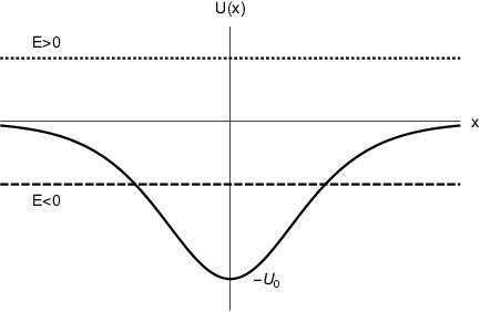
Figure 7: The Pöschl - Teller potential. If the particle has positive energy its motion is unbounded, else () the spectrum of the energy becomes discrete. By comparing (68) and (69), the analogy is obvious. The constants , are all set to unity, while and the “energy” of the particle of our case becomes . It is negative and thus it results in a finite number of bound states. Additionally we have and the eigenvalues follow the restriction
(72) The wave function solving (68) is given in terms of the associated Legendre polynomials Poschl3; SDong, which satisfy the normalization condition
(73) The weight factor inside the integral of (73) is exactly what we obtain from the measure choice we did in (52). If we concentrate on the dependent part we have
(74) where in the above the subsequent changes , and have been used.
In what regards both of the previous cases, the dependence of the wave function from the scale factor is decided from the remaining Wheeler-DeWitt equation (56) and its solution (62), which for and under a change of variables , it can be written as
| (75) |
where and are linear combinations of the integration constants and of (62) respectively. We remind here the basic formulas connecting the Bessel functions, , , , for being generally complex variables.
For the wave function we choose the first branch of the solution, since it is well known that the spherical Bessel function of the first kind satisfies the orthogonality relation
| (76) |
In our case which is allowed a continuous set of values. Notice that again the natural measure of (52) is the one resulting in the needed weight in the integral (76) since, by concentrating on the dependence, we have
| (77) |
Once more the overall multiplicative numerical factor is irrelevant since it can be absorbed in the normalization constant.
In order to sum the above results we write final wavefunctions. In the first case where we have
| (78) |
where the quantum numbers follow the restrictions
| (79) |
and the normalization constant is
| (80) |
The measure used is and it differs from what we introduced in (52) by a multiplicative constant. We remind here that the variable is related to through . For simplicity we use directly in order to have a simpler expression for , i.e. not having to include in it an additional numerical factor.44 4 Another reason for not using directly the of (52) is because the latter was written given a real variable . In the two cases considered in this section is taken to be complex, thus we could not have adopted exactly the same expression. Nevertheless the difference is just an overall constant.
The second case in which leads to a wave function
| (81) |
where the following relations hold
| (82) |
and the normalization constant is
| (83) |
Notice that due to the (82), the in the above relation is also a natural number. For the measure in this case we have and as previously the difference with the of (52) is once more a multiplicative constant.
We have thus demonstrated, that the classical situation, which is obtained by two distinct choices of parameters, corresponds at the quantum level to “bound states”. That is, a discrete spectrum for the quantum numbers and , although the quantum procedure in the two cases is different (as also the quantum conditions on ). Additionally, in our formulation of the system, the cosmological constant can be perceived as a quantum eigenvalue from the Wheeler-DeWitt equation, which however has a continuous spectrum and it is normalized to the Dirac delta.
Finally it is interesting to remark that the eigenvalue has its classical equivalent on having which corresponds to the de Sitter universe (remember that is the eigenvalue of whose classical counterpart’s on mass shell value is given in (64)).
V.2 The case
From the classical solution we know that (64) is negative whenever both and are real and we saw that this corresponds to what we characterized as the quintessence epoch. In this case, we can parameterize the quantum number as , . Then, the eigenvalue remains real but it is exclusively negative. We have of course the same general solution (59) of the eigenvalue equation (58), only that now is real and we have to take into account the orthogonality relation Van
| (84) |
where denotes the gamma functions that extend the factorial definition.
The spectrum of is continuous and the system corresponds to “free” states. In what regards (84), we have to notice that in the literature there appear two different definitions of the associated Legendre function. Under the first definition the function is real in the region , which is our domain of integration. The second definition differs from the first by a multiplicative constant factor of . However, when the product is used, such a constant phase is eliminated. So, as far as the probability is concerned, there is no distinction between the two definitions. For simplicity and to avoid complex conjugates we use here the one according to which is a real function.
The only thing that remains is to decide which linear combination of the solution of (75) is appropriate to serve in our description. In this case the spherical Bessel is of complex order . We may use the transformation in (75) and derive the solution
| (85) |
where , are constants of integration proportional to the , of (75) respectively. In the case of imaginary order an interesting linear combination of the solution can be distinguished in the form of the function Dunster
| (86) |
where is related to linear combinations of the previous constants, and , and which serves to normalize the wave function. By definition the is a real function. What is more, a normalization condition in terms of a Dirac delta can also be derived (see appendix B).
Interestingly enough, the states spanned by different values of are not necessarily orthogonal. It can be deducted however (see once more appendix B) that the orthogonality condition between two states characterized by eigenvalues and requires either or
| (87) |
The requirement emerges from the need to cancel the lower limit of the integral when the inner product is used. However, it has been shown that if a different linear combination of the solution is adopted, such a contribution can be avoided, see Gryb; Gielen. According to the choice of the solution we make here the dependence of the wave function is (remember that is the variable related to the scale factor )
| (88) |
and thus the full wave function becomes
| (89) |
where , and is restricted by (87), while the normalization constant reads
| (90) |
under the inner product of , where .
In contrast to what we found in the phantom epoch, , which is described by a bounded set of states, the quintessence era is characterized by a continuous spectrum for . We have to note that the eigenvalue remains discrete in both cases since the sign of makes no difference for it.
Lastly we want to address what happens at the classical singularity, which is present in the quintessence epoch geometry. We recognize that there is no general consensus on what constitutes a singularity avoidance at the quantum level, since there exist various different methods of quantization and in many cases even different interpretations of the wave function and of the corresponding probability within the same theory. However, a reasonable assumption is to not have divergences in the region in which a classically problematic point corresponds Kiefer. In our case this happens when when we consider the quintessence case. From our choice of inner product we can see that the probability amplitude for the dependent part of the wave function is analogous to
| (91) |
We can see that in both cases the limit leads to . In the first branch of , corresponding classically to the phantom solution, we have at the small limit: . So, clearly goes to zero as , even though classically we have no particular problem at the given point. For the second branch, which at the classical level relates to the quintessence solution, the behaviour of the function for small arguments can be found in (103) of appendix B. It oscillates strongly but it remains finite. Thus the factor in the second part of (91) dominates sending to zero as we approach . We interpret this result as a zero transition probability to the problematic point from a neighboring point , which we consider to be a good sign for avoiding the singularity.
VI Conclusions
In this work we consider a two-scalar field cosmology. Specifically, we assume the contribution in the Einstein field equations only by the kinetic parts of two interacting scalar fields as in the -attractor model, where the fields are also minimally coupled to gravity. In addition, we assume that the scalar field potential is constant and thus plays the role of a cosmological constant. In a FLRW background space we derived the generic classical analytic solution of this model.
In the case of a spatially flat universe and for a specific value of one of the free parameters of the model, we were able to write the analytic solution in closed form. For that specific case we studied the behaviour of the physical parameters for various ranges of the integration constants of the problem. Surprisingly, we found that it is possible to describe a quintessence epoch, a phantom epoch or even a quintom model depending on the values of the free parameters. In all of the above configurations appropriate domains of deinition for the parameters can be found so that the physical quantities are real functions. The quintessence solution describes a universe with an initial singularity, in contrast to the phantom (or the quintom) solution which results in a bouncing universe. In addition, all of the solutions have a common future: at late times they give the de Sitter universe as an attractor.
Successively, we applied the minisuperspace approach to perform a canonical quantization and write the Wheeler-DeWitt equation of quantum cosmology. We showed how to construct quantum operators from the classical conservation laws, which are used as additional constraints in order to calculate the wave function of the universe. We perform a preliminary analysis for the generic case and we focus the construction of a valid set of states for the particular configuration which we investigated at the classical level and which corresponds to the spatially flat FLRW universe. We demonstrate how different eigenvalues of the quantum operators are related with the two different behaviours of the classical solutions, that is, different quantum states describe distinct classical behaviours.
It is very interesting the fact that an expansion characterized by a phantom behaviour, i.e. is related to a bounded set of states, while on the other hand the quintessence epoch, that is; corresponds to free states for the universe. In this sense we see a hint of realization of how canonical quantization of gravity, as initially introduced in the seminal paper by B. S. DeWitt DeWitt, tries to take form as a quantization in the space of geometries, with different sets of states being linked to different classical geometries. Another important remark is that the resulting wave function leads to a resolution of the classical singularity (when the latter is present) in the sense that the probability amplitude tends to zero at the problematic point.
Appendix A
Here we give the details on how to arrive from (23) to (24), when and the gauge choice has been made. Solution (23) is derived for and when we set the aforementioned values for and it reads
| (92) |
First, we reparametrize the constant as and exploit the identity
| (93) |
in order to write
| (94) |
With a subsequent reparametrization of the constant as , we can use (94) to express the cube of the scale factor, , as
| (95) |
At this point note that in place of we introduced two constants, and . We are going to fix appropriately the former, while the latter remains arbitrary. We proceed by reparametrizing and fixing in such a manner so that we have
| (96) |
where is the newly introduced constant in place of . As a result (95) becomes
| (97) |
We can exploit the invariance of the solution under time translations to eliminate one of the two additive constants, either or . For example, we can perform a time translation and at the same time introduce a new constant . Then only enters the expressions for , and , while just appears additively in . By demanding the boundary condition we can set to be zero. We avoid all this procedure and straightforwardly set in (97). By successively taking the cubic root of (97), we are finally led to equation (24).
Appendix B
Let us start from the Bessel equation of our case which is satisfied by the solution (85)
| (98) |
where as an eigenvalue we have set and with we denote the solution that we use, the real function
| (99) |
We follow the usual procedure with which we derive orthogonality conditions in a Sturm - Liouville problem: We take the equation for a different eigenvalue
| (100) |
We multiply the first equation with and the second with and subsequently we subtract by parts. As a result we arrive at
| (101) |
from where integration over the half line leads to
| (102) |
If we take into account the approximate expressions for
| (103) |
where is a specific constant depending on , then it is easy to see that
| (104) |
and
| (105) |
This last term gives a delta function when interpreted in a distributional sense, as we are going to see below. However, we may notice that the other contribution in (102), given by (104) is not zero. This means that the states with are not necessarily orthogonal.
Only for or for those eigenvalues that satisfy
| (106) |
is the term zero.
Now, for (105) and its connection to the delta distribution, we need to remember the Riemann-Lebesgue lemma
| (107) |
and the representation of the Dirac delta
| (108) |
for an appropriate test function . Then, (102) leads us to
| (109) |
As we noticed before, the states that are orthogonal are characterized by , which holds either for or under the validity of (106). Otherwise, if , we notice that the limit
| (110) |
is finite.
References
- (1) M. Tegmark et al., Astrophys. J. 606 702 (2004)
- (2) M. Kowalski et al., Astrophys. J. 686 749 (2008)
- (3) E. Komatsu et al., Astrophys. J. Suppl. Ser. 180 330 (2009)
- (4) P. A. R. Ade et al., Astron. Astroph. 571 A15 (2014)
- (5) N. Aghanim et al., Planck 2018 results. VI. Cosmological parameters, [arXiv:1807.06209]
- (6) A. Guth, Phys. Rev. D 23, 347 (1981)
- (7) B. Ratra and P. J. E Peebles, Phys. Rev. D 37, 3406 (1988)
- (8) J.D. Barrow and P. Saich, Class. Quant. Grav. 10, 279 (1993)
- (9) S. Weinberg, Rev. Mod. Phys. 61, 1 (1989)
- (10) T. Padmanabhan, Phys. Rept. 380, 235 (2003)
- (11) S. Basilakos, N. E. Mavromatos and J. Sola, JCAP 1912, 025 (2019)
- (12) J. Sola, A. Gomez-Valent, J. de Cruz Perez, Mod. Phys. Lett. A 32, 1750054 (2017)
- (13) S. Pan, J. Haro, A. Paliathanasis, R. J. Slagter, MNRAS 460, 1445 (2016)
- (14) J.C. Fabris, T.C.C. Guio, M.H. Daouda and O.F. Piattella, Grav. Cosmol. 17, 259 (2011)
- (15) J. D. Barrow and A. Paliathanasis, Phys. Rev. D 94, 083518 (2016)
- (16) C. Brans and R. H. Dicke, Phys. Rev. 124, 195 (1961)
- (17) T. Clifton, P. G. Ferreira, A. Padilla and C. Skordis, Phys. Rept. 513, 1 (2012)
- (18) H.A. Buchdahl, Mon. Not. Roy. Astron. Soc. 150, 1 (1970)
- (19) B. Li, J. D. Barrow and D.F. Mota, Phys. Rev. D 76, 044027 (2007)
- (20) R. Ferraro and F. Fiorini, Phys. Rev. D 78, 124019 (2008)
- (21) A. Paliathanasis, J. D. Barrow and P.G.L. Leach, Phys. Rev. D 94, 023525 (2016)
- (22) D. Lovelock, J. Math. Phys 12, 498 (1971)
- (23) S. Nojiri and S. D. Odintsov, Phys. Rept. 505, 59 (2011)
- (24) S. Nojiri, S. D. Odintsov and V. K. Oikonomou, Phys. Rept. 692, 1 (2017)
- (25) A. A. Starobinsky, Phys. Lett. B 91, 90 (1980)
- (26) A. Paliathanasis and P. G. L. Leach, Phys. Lett. A 380, 2815 (2016)
- (27) N. Dimakis, A. Giacomini and A. Paliathanasis, EPJC 78, 751 (2018)
- (28) S. D. Odintsov and V. K. Oikonomou, Phys. Rev. D 92, 024016 (2015)
- (29) V. Faraoni and E. Gunzig, Int. J. Theor. Phys. 37, 217 (1999)
- (30) M. Postma and M. Volponi, Phys. Rev. D 90, 103516 (2014)
- (31) A. de la Macorra and G. Piccinelli, Phys. Rev. D 61, 123503 (2000)
- (32) V. B. Johri, Class. Quantum Grav. 19, 5959 (2002)
- (33) A. Paliathanasis, M. Tsamparlis and S. Basilakos, Phys. Rev. D 90, 103524 (2014)
- (34) T. Gonzales, G. Leon and I. Quiros, Class. Quantum Grav. 23, 3165 (2006)
- (35) G. Leon and O. F. Silva, Generalized scalar field cosmologies [arXiv:1912.09856]
- (36) E. Piedipalumbo, P. Scudellaro, G. Esposito and C. Rubano, Gen. Rel. Grav. 44, 2611 (2012)
- (37) A. Yu. Kamenshchik, E. O. Pozdeeva, A. Tronconi, G. Venturi, and S.Yu. Vernov, fields, Class. Quantum Grav. 31, 105003 (2014)
- (38) D. L. Shafer and D. Huterer, Phys. Rev. D 89, 063510 (2014)
- (39) S. Nesseris and L. Perivolaropoulos, JCAP 0701, 018 (2007)
- (40) I. Leanizbarrutia and D. Sáez-Gómez, Phys. Rev. D 90, 063508 (2014)
- (41) W. Yang, S. Pan, A. Paliathanasis, S. Ghosh and Y. Wu, MNRAS 490, 2071 (2019)
- (42) W. Yang, N. Banerjee, A. Paliathanasis and S. Pan, Physics of the Dark Energy 26, 100383 (2019)
- (43) F. K. Anagnostopoulos, S. Basilakos, G. Kofinas and V. Zarikas, 1902, 053 (2019)
- (44) R. R. Caldwell, Phys. Lett. B 545, 23 (2002)
- (45) S. Nojiri, S.D Odintsov, V.K. Oikonomou and E.N. Saridakis, JCAP 1509, 044 (2015)
- (46) A. V. Astashenok, S. Nojiri, S. D. Odintsov and A. V. Yurov, Phys. Lett. B 709, 396 (2012)
- (47) M. Bouhmadi-Lopez and J.A. Jimenez Madrid, JCAP 0505, 005 (2005)
- (48) A. Yurov, Eur. Phys. J. Plus 126, 132 (2011)
- (49) M. Sami and A. Toporensky, Mod. Phys. Lett. A 19, 1509 (2004)
- (50) W. Hu, Phys. Rev. D 71, 047301 (2005)
- (51) Y.-F. Cai, E. N. Saridakis, M. R. Setare and J.-Q. Xia, Phys. Rept. 493, 1 (2010)
- (52) L. P. Chimento, M. Forte, R. Lazkoz and M. G. Richarte, Phys. Rev. D 79, 043502 (2009)
- (53) J. Socorro and O.E. Nunez, Eur. Phys. J. Plus 132, 168 (2017)
- (54) V. Sivanesan, Phys. Rev. D 90, 104006 (2014)
- (55) A. Paliathanasis, Gen. Rel. Grav. 51, 101 (2019)
- (56) S. V. Chervon, Russ. Phys. J. 38, 539 (1995)
- (57) S. V. Ketov, Quantum Non-linear Sigma Models, Springer-Verlag, Berlin, (2000).
- (58) J. Lee, T.H. Lee, T. Moon and P. Oh, Phys. Rev. D 80, 065016 (2009)
- (59) K.-i Maeda, S. Mizuno and R. Tozuka, Phys. Rev. D 98, 123530 (2018)
- (60) C. Garcia-Garcia, E. V. Linder, P. Ruiz-Lapuente and M. Zumalacarregui, JCAP 1808, 022 (2018)
- (61) A. Alho and C. Uggla, Phys. Rev. D 95, 083517 (2017)
- (62) P. Christodoulidis, D. Roest and E.I. Sfakianakis, JCAP 1911, 002 (2019)
- (63) K. Dimopoulos and C. Owen, JCAP 1706, 027 (2017)
- (64) T. Krajewski, K. Turzynski and M. Wieczorek, EPJC 79, 654 (2019)
- (65) Y. Akrami, R. Kallosh, A. Linde and V. Vardanyan, JCAP 1806, 041 (2018)
- (66) J. Socorro, S. Pérez-Payan, R. Hernández, A. Espinoza-García and L.R. Díaz-Barrón, Classical and quantum exact solutions for a FRW in chiral like cosmology [arXiv:2012.11108]
- (67) B.S. De Witt, Phys. Rev. 60, 1113 (1967)
- (68) A. Karagiorgos, T. Pailas, N. Dimakis, Petros A. Terzis, T. Christodoulakis, JCAP 1904, 006 (2019)
- (69) T. Christodoulakis, N. Dimakis, P.A Terzis and G. Doulis, Phys. Rev. D 90, 024052 (2014)
- (70) T. Pailas, Quantum rep. 2(3), 414 (2020)
- (71) A. Zampeli, T. Pailas, P.A. Terzis and T. Christodoulakis, JCAP 1605, 066 (2016)
- (72) T. Christodoulakis, N. Dimakis and Petros A. Terzis, J. Phys. A: Math. theor. 47, 095202 (2014)
- (73) S. Capozziello, M. De Laurentis and S.D. Odintsov, Eur. Phys. J. C 72 2068 (2012)
- (74) A. Paliathanasis, M. Tsamparlis, S. Basilakos and J.D. Barrow, Phys. Rev D 93, 043528 (2016)
- (75) J. Maharana, Phys. Lett. B 549 7 (2002)
- (76) J. Maharana, Int. J. Mod. Phys. A 20 1441 (2005)
- (77) R. Cordero and R. D. Mota, Eur. Phys. J. Plus 135, 78 (2020)
- (78) A. Paliathanasis and M. Tsamparlis, Phys. Rev D 90, 043529 (2014)
- (79) N. Dimakis, A. Paliathanasis, P.A. Terzis and T. Christodoulakis, EPJC 79, 618 (2019)
- (80) H. Lam and T. Prokopec, Phys. Lett. B 775, (2017) 311
- (81) P. A. M. Dirac, Canad. J. Math 2, 129 (1950)
- (82) J. Anderson and P. Bergmann, Phys. Rev. 83, 1018 (1951)
- (83) P. A. M. Dirac, Lectures on Quantum Mechanics, Yeshiva University, Academic Press, New York (1964)
- (84) K. Sundermeyer, Constrained Dynamics, Springer - Verlag, Berlin, Heidelberg, New York (1982)
- (85) T. Christodoulakis and J. Zanelli, Nuovo Cim. B 93, 1 (1986)
- (86) J. P. Michel, F. Radoux and J. Šilhan, SIGMA 10, 016 (2014)
- (87) T. Christodoulakis, N. Dimakis, Petros A. Terzis, G. Doulis, Th. Grammenos, E. Melas and A. Spanou, J. Geom. Phys. 71, 127 (2013)
- (88) N. Dimakis, A. Karagiorgos, T. Pailas, Petros A. Terzis, T. Christodoulakis, Phys. Rev. D 95, 086016 (2017)
- (89) A. Karagiorgos, T. Pailas, N. Dimakis, Petros A. Terzis, T. Christodoulakis, JCAP 1803, 030 (2018)
- (90) G. Pöschl and E. Teller, Zeitschrift für Physik 83, 143 (1933)
- (91) L. D. Landau and E. M. Lifshitz, “Quantum Mecanics (Non-relativistic Theory)”, 3rd Edition, Pergamon Press, Oxford, New York, Beijing (1977)
- (92) Y. You, Fa-Lin Lu, Dong-Sheng Sun, Chang-Yuan Chen and Shi-Hai Dong, Few-Body Systems 54, 2125 (2013)
- (93) M. M. Nieto, Phys. Rev. A 17, 1273 (1978)
- (94) S.-H. Dong, “Factorization Methods in Quantum Mechanics”, Springer, Dordrecht, The Netherlands (2007)
- (95) R. G. Van Nostrand, Journal of Mathematics and Physics 33, 276 (1954)
- (96) T. M. Dunster, SIAM J. Math. Anal. 21, 995 (1990)
- (97) S. Gryb and K. P. Y. Thébault, Class. Quantum Grav. 36, 035009 (2019)
- (98) S. Gielen and L. Menéndez-Pidal, Class. Quantum Grav. 37, 205018 (2020)
- (99) C. Kiefer, Ann. Phys. (Berlin) 19, No. 3-5, 211 (2010)