Nonequilibrium transport and phase transitions
in driven diffusion of interacting particles
Abstract
Driven diffusive systems constitute paradigmatic models of nonequilibrium physics. Among them, a driven lattice gas known as the asymmetric simple exclusion process (ASEP) is the most prominent example for which many intriguing exact results have been obtained. After summarizing key findings, including the mapping of the ASEP to quantum spin chains, we discuss the recently introduced Brownian asymmetric simple exclusion process (BASEP) as a related class of driven diffusive system with continuous space dynamics. In the BASEP, driven Brownian motion of hardcore-interacting particles through one-dimensional periodic potentials is considered. We study whether current-density relations of the BASEP can be considered as generic for arbitrary periodic potentials and whether repulsive particle interactions other than hardcore lead to similar results. Our findings suggest that shapes of current-density relations are generic for single-well periodic potentials and can always be attributed to the interplay of a barrier reduction, blocking and exchange symmetry effect. This implies that in general up to five different phases of nonequilibrium steady states are possible for such potentials. The phases can occur in systems coupled to particle reservoirs, where the bulk density is the order parameter. For multiple-well periodic potentials, more complex current-density relations are possible and more phases can appear. Taking a repulsive Yukawa potential as an example, we show that the effects of barrier reduction and blocking on the current are also present. The exchange symmetry effect requires hardcore interactions and we demonstrate that it can still be identified when hardcore interactions are combined with weak Yukawa interactions. The robustness of the collective dynamics in the BASEP with respect to variations of model details can be a key feature for a successful observation of the predicted current-density relations in actual physical systems.
I Introduction
Driven diffusive systems of interacting particles constitute an important class of systems to study fundamental aspects of nonequilibrium physics. This holds in particular for one-dimensional models, where exact analytical derivations are possible or reliable approximations are known, for example, when information about exact equilibrium properties can be utilized for the treatment of nonequilibrium states.
A prominent model in the field of driven diffusive systems is the asymmetric simple exclusion process (ASEP), where particles hop between nearest-neighbor sites of a lattice with a bias in one direction and where the sole interaction between particles is a mutual site exclusion, implying that a lattice site cannot be occupied by more than one particle Derrida 1998; Schütz 2001. In the ASEP on a one-dimensional lattice with sites and periodic boundary conditions, i.e. a ring of sites, particles jump to vacant nearest-neighbor sites with rates and in clockwise and counterclockwise direction, respectively, where for a bias in clockwise direction. In a corresponding open system with sites, where the leftmost and rightmost lattice site can exchange particles with reservoirs L and R, respectively, additional rates , and , specify the corresponding rates for particle injection and ejection. Many properties of the ASEP can be inferred from the even simpler totally asymmetric simple exclusion process (TASEP) with unidirectional transport ().
Stochastic processes in driven lattice gases are described by a master equation for the probabilities of particle configurations, which can be viewed also as the occupation number representation of a Schrödinger equation in imaginary time Gwa and Spohn 1992; Sandow and Trimper 1993. This leads to some interesting connections to quantum systems with in general non-Hermitian Hamilton operator Gwa and Spohn 1992; Sandow 1994; Henkel and Schütz 1994; Schütz 2001. As an example, we recapitulate in the Appendix the connection of the ASEP with periodic boundary conditions to the quantum spin chain with non-Hermitian boundary conditions Henkel and Schütz 1994. Spin chains are often used to study fundamental aspects of nonequilibrium quantum physics. Several examples related to current problems, in particular to questions of equilibration in non-integrable spin chain models, can be found in this special issue.
The ASEP has been intensively studied in the past. Let us summarize
here some of the most important findings for the ASEP and variants of
it:
- –
Using the Bethe ansatz for corresponding quantum spin chain models, or a construction in terms of matrix product states, exact results for microstate distributions in nonequilibrium steady states (NESS) could be derived Derrida 1998; Schütz 2001; Blythe and Evans 2007. Matrix product states in principle exist for driven lattice gases with arbitrary nearest-neighbor interactions Krebs and Sandow 1997, although their explicit construction may be difficult.
- –
Based on the exact approaches for deriving distribution of microstates in NESS, large deviation functions for fluctuations of time-averaged densities and currents were derived Derrida and Lebowitz 1998; Derrida et al. 2002; Krapivsky et al. 2014. They have been computed also for coarse-grained descriptions by the macroscopic fluctuation theory Bertini et al. 2015. Large deviation functions are argued to play a similar role for time-averaged quantities in NESS as the free energy in equilibrium systems Touchette 2009. They can exhibit singularities Bertini et al. 2005; Bodineau and Derrida 2005; Appert-Rolland et al. 2008; Baek et al. 2017, sometimes referred to as “dynamical phase transitions”, which for certain classes of systems are caused by a violation of an “additivity principle” Bodineau and Derrida 2004.
- –
The Bethe ansatz turned out to be a valuable tool also for deriving microstate distributions of non-steady states Schütz 1997; Tracy and Widom 2008a. The propagator for the microstate time evolution in the ASEP was related to integrated Fredholm determinants Tracy and Widom 2008b and led to the derivation of the Tracy-Widom distribution of random matrix theory for the asymptotic behavior in case of a step initial condition Tracy and Widom 2009. This result generalized an earlier one derived for the TASEP Johansson 2000 and proved that the propagation of density fluctuations in the ASEP belongs to the Kardar-Parisi-Zhang (KPZ) universality class Kardar et al. 1986.
- –
In open systems coupled to particle reservoirs, phase transitions between NESS occur Krug 1991; Schütz and Domany 1993; Kolomeisky et al. 1998; Brzank and Schütz 2007, where, upon change of control parameters characterizing the system-reservoir couplings, the bulk density changes discontinuously, or its derivative with respect to the control parameters. Knowing the density dependence of the steady-state bulk current , e.g. from results for a system with periodic boundary conditions, all possible NESS phases with bulk density are predicted by the extremal current principles Krug 1991; Kolomeisky et al. 1998; Popkov and Schütz 1999
(1) Here and can be any densities bounding a monotonically varying region encompassing the plateau part with bulk density (which may strictly exist only in the thermodynamic limit of infinite system size). Which of the phases predicted by Eq. (1) really occurs for a given control scheme of system-reservoir couplings, is given by the dependence of and on respective control parameters.
The extremal current principles can be reasoned based on the consideration of shock front motions Kolomeisky et al. 1998; Popkov and Schütz 1999; Hager et al. 2001, or by resorting to a decomposition of the steady-state current into its drift and diffusive part inside the region of monotonically varying density profile Krug 1991. Because these reasonings do not require specific properties of the ASEP, they are quite generally valid for driven diffusive systems coupled to particle reservoirs. This includes driven lattice gases with interactions other than site exclusion Antal and Schütz 2000; Hager et al. 2001; Dierl et al. 2012; Dierl et al. 2013, systems with continuous space-dynamics and systems with periodic space structure and/or time-periodic driving, when considering period-averaged densities Dierl et al. 2014. For specific system-reservoir couplings termed “bulk-adapted” it is possible to parameterize the exchange of particles by reservoir densities such that all possible NESS phases must appear. The bulk-adapted couplings can be determined by a general method for driven lattice gases with short-range interactions Dierl et al. 2013; Dierl et al. 2014.
- –
For random and non-Poissonian hopping rates, Bose-Einstein type condensations of vacancies can occur in front of the slowest particle with smallest jump rate Evans 1996; Concannon and Blythe 2014.
- –
Coarse-grained continuum descriptions of the ASEP and of multilane variants Popkov and Salerno 2004 give rise to an infinite discrete family of nonequilibrium universality classes in nonlinear hydrodynamics, where density fluctuations spread in time by power laws with exponents given by the Kepler ratios of consecutive Fibonacci numbers Popkov et al. 2015. This includes the KPZ class, for which an exact expression for the scaling function was derived Prähofer and Spohn 2004. Predictions of the theory of fluctuating nonlinear hydrodynamics were recently confirmed in an exact treatment by considering a two-species exclusion process Chen et al. 2018.
As for applications, the ASEP appears as a basic building block in manifold descriptions of biological traffic Schadschneider et al. 2010; Chou et al. 2011. In fact, the ASEP was introduced first to describe protein synthesis by ribosomes MacDonald et al. 1968, and it is frequently used in connection with the motion of motor proteins along microtubules or actin tracks Kolomeisky 2013; Appert-Rolland et al. 2015. An in-vitro study with fluorescently labeled single-headed kinesin motors moving along a microtubule provided experimental evidence for a state of coexisting phases with different motor densities Nishinari et al. 2005. Other applications concern vehicular traffic Appert-Rolland et al. 2011; Foulaadvand and Maass 2016, diffusion of ions through cell membranes Hille 2001 and of molecules through nanopores Cheng and Bowers 2007; Dvoyashkin et al. 2014, and electron transport along molecular wires in the incoherent classical limit Nitzan 2001; Berlin et al. 2001. However, a direct experimental realization of the ASEP is difficult, because of its discrete nature. Hence, it is important to see whether the nonequilibrium physics in the ASEP is reflected in models with continuous space dynamics.
For a single particle, it is well known that effective hopping transport emerges from an overdamped Brownian motion in a periodic potential with amplitude much larger than the thermal energy. The particle can be viewed to jump between neighboring wells on a coarse-grained time scale with a rate determined by the inverse Kramers time Risken 1985. One is thus led to ask whether the driven diffusion of many hardcore interacting particles in a periodic energy landscape can reflect the driven lattice gas dynamics in the ASEP. To answer this question, we recently introduced a corresponding class of nonequilibrium processes termed Brownian ASEP (BASEP) Lips et al. 2018; Lips et al. 2019, where hard spheres with diameter are driven through a periodic potential with wavelength by a constant drag force . For a sinusoidal external potential, we found that the current-density relation of the ASEP is indeed recaptured in the BASEP, but only for a limited range of particle diameters . For other , quite different behaviors are obtained.
The nonequilibrium physics of the BASEP should be explorable directly by experiment, for example in setups utilizing advanced techniques of microfluidics and optical and/or magnetic micromanipulation Arzola et al. 2017; Skaug et al. 2018; Schwemmer et al. 2018; Stoop et al. 2019; Misiunas and Keyser 2019. This includes arrangements where the particles are driven by traveling-wave potentials Straube and Tierno 2013. Many of the new collective transport properties seen in the BASEP can be even identified by studying local dynamics of individual transitions between potential wells Ryabov et al. 2019.
In this work we address the question how the current-density relations found for the BASEP in a sinusoidal external potential are affected when considering different external potentials and short-range interactions other than hardcore exclusions. Our investigation for the different external potentials are carried out based on the small-driving approximation introduced in Refs. Lips et al. 2018 and Lips et al. 2019. With respect to short-range interactions other than hardcore exclusions, we focus on a Yukawa pair potential. It is shown that the current-density relation for single-well periodic potentials and for the Yukawa interaction has similar features as that of the BASEP. This suggests that the BASEP can serve as a reference model for a wide class of external periodic potentials and pair interactions.
In addition we extend a former analysis to prove that current reversals cannot occur in systems driven by a constant drag and by traveling waves. These proofs are based on an exact calculation of the total entropy production in corresponding NESS for particles with arbitrary pair interactions. Current reversals refer to steady states, where particle flow is opposite to the external bias. They were reported for lattice models Jain et al. 2007; Slanina 2009a; Slanina 2009b; Chaudhuri and Dhar 2011; Dierl et al. 2014 and were recently found experimentally in a rocking Brownian motor Schwemmer et al. 2018. Their absence in traveling-wave driven systems was conjectured based on simulation results and a perturbative expansion of the single-particle density in the NESS around its period-averaged value Chaudhuri et al. 2015.
The paper is organized as follows. In Sec. II we present an analytical treatment of densities and currents for the overdamped one-dimensional Brownian motion of particles with arbitrary pair interactions. This section partly summarizes results presented earlier Lips et al. 2018; Lips et al. 2019 and introduces the small-driving approximation used subsequently for our investigation of hardcore interacting particles. It also contains our proofs on the absence of current reversals for general pair interactions. In Sec. III we outline our findings for the BASEP with sinusoidal external potential, and in Sec. IV we contrast them with results for a Kronig-Penney and triple-well periodic potential. In Sec. V we discuss our results for the Yukawa interaction. Section VI concludes the paper with a summary and outlook.
II Current-density relations: Analytical results
The overdamped single-file Brownian motion of particles in a periodic potential with pair interaction under a constant drag force is described by the Langevin equations
| (2) |
where and are the bare mobility and diffusion coefficient, is the thermal energy, and is the interaction force on the th particle. The are independent and -correlated Gaussian white noise processes with zero mean and unit variance, and . Unless noted otherwise, we consider closed systems with periodic boundary conditions, which means that the particles are dragged along a ring.
Hardcore interactions imply the boundary conditions , i.e. overlaps between neighboring particles are forbidden. For the BASEP with only hardcore interactions, these boundary conditions must be taken into account, while the interaction force can be set to zero in Eq. (2). We define the density as a (dimensionless) filling factor of the potential wells, i.e. by , where denotes the total number of periods of . The system length is and the number density is . For hardcore interacting particles of size , the filling factor has the upper bound .
The joint probability function (PDF) of the particle center coordinates evolves in time according to the -particle Smoluchowski equation 11 1 To implement the periodic boundary conditions, we assume an ordered initial configuration , and introduce two fictive particles with enslaved coordinates and , which implies .,
| (3) |
where the divergence operator acts on the probability current vector with the th component given by
| (4) | ||||
The first term describes the drift probability current caused by all forces acting on the th particle and the second term gives the diffusive current. The interaction force is assumed to be conservative and due to pair interactions , i.e. with
| (5) |
Additional hardcore interactions are not included in the potential (5) but are incorporated into the dynamics by requiring no-flux (reflecting) boundary conditions
| (6) |
if neighboring particles hit each other. These boundary conditions ensure conservation of an initial ordering of the particle positions for all times.
II.1 Exact current-density relation
The local density is
| (7) |
where the average is taken with respect to the solution of the Smoluchowski equation (3) subject to some initial condition. It satisfies the continuity equation
| (8) |
with the particle current density given by Lips et al. 2018
| (9) |
Here we introduced the total external force
| (10) |
The local interaction force in Eq. (9) is given by
| (11) |
where
| (12) |
is the two-point local density, and is the interaction force of a particle at position on a particle at position . It can by expressed as a sum of two distinct contributions:
| (13) |
The first term is due to a positive and a negative force, if a particle is in contact with other particles at positions and , respectively. We note that the -functions should not be interpreted as a derivative of a rectangular potential barrier of height . Instead, they are a consequence of the noncrossing boundary conditions (6) Lips et al. 2018. The amplitude in front of the -functions must be an energy on dimensional reasons, for which is the only relevant scale. It corresponds to the typical collision energy due to the thermal noise. The second term in Eq. (13) is the force due to the interaction potential (5).
In the steady state of a closed system with periodic boundary conditions, the density profile is time-independent and periodic, and the current constant everywhere in the system. It follows directly from Eq. (9) Lips et al. 2018
| (14) |
Up to this point no approximation has been made. The exact value of the steady-state current (14) depends on both and the steady-state limit of the two-point density (12). However, derivation of the two densities in NESS represents a challenging problem, which can be solved in a few special cases only. Therefore, to proceed further, we need to develop an appropriate approximate theory.
II.2 Small-driving approximation
For hardcore interactions, the small-driving approximation (SDA) turned out to be particularly successful in capturing qualitative behaviors of Lips et al. 2019. The approximation is carried out in two steps. Firstly, we linearize the current (14) with respect to ,
| (15) |
where the response coefficient reads
| (16) |
and, secondly, we approximate the linear-response expression (15) by setting .
The ad-hoc approximation works well in an extended region of particle sizes except for a narrow range Lips et al. 2019. The equilibrium density profile is obtained by minimizing the exact density functional for hard rods Percus 1976,
| (17) |
where is the chemical potential, and
| (18) |
The minimization yields the structure equation
| (19) | ||||
which we discretized and solved numerically under periodic boundary conditions []. The chemical potential was adjusted to give the desired global density (filling factor) .
II.3 Entropy production and absence of current reversals
Theory for hardcore interacting particles with was the subject of our previous works on the BASEP Lips et al. 2018; Ryabov et al. 2019; Lips et al. 2019. Here we extend the analysis to nonzero . We start with considerations related to the total entropy production:
| (20) |
where and are the entropy production in the system and surrounding medium.
For calculating the time derivative of we can replace the time derivative of the PDF by the divergence of the current according to (3). After integrating by parts of each individual term of the divergence, we get
| (21) |
where is the space of all system microstates consistent with the hardcore constraints. As the next step, we replace via Eq. (4), which gives us two terms
| (22) |
Here we have introduced the total force with components . The first term is always positive and equal to the total entropy production Seifert 2012. The second term, proportional to the mean dissipated power, is the entropy production in the medium.
In the steady state, the system entropy is constant, , and the total entropy production equal to the entropy produced in the surrounding medium:
| (23) | ||||
Here, each single-particle term simplifies after introducing the current density , of the th particle, and by using that in the steady state,
| (24) |
The sum over all interaction forces in Eq. (23) yields, after integration by parts,
| (25) |
Because the divergence of the current is zero in the steady state, this term vanishes. From Eqs. (23) and (24) we thus obtain the total entropy production in the Onsager form (current times thermodynamic force)
| (26) |
It is extensive in the system size and the numerator equals the mean heat dissipated at any point of the system in the steady state. As a consequence of the inequality in (26), the steady state current must have the same sign as the drag force .
II.4 Entropy production in traveling-wave driven systems and current bounds
A feasible way to verify BASEP current-density relations in a laboratory is to consider an equivalent ring system with the traveling-wave (TW) external periodic potential and Šiler et al. 2008; Straube and Tierno 2013; Di Leonardo et al. 2007; Curran et al. 2010; Šiler et al. 2012. In such a TW system, the th compomnent of the probability current vector is
| (27) | ||||
Under a Galilean transformation
| (28) |
the TW system maps to the corresponding BASEP with potential and constant drag force
| (29) |
provided the pair interaction potential is a function of the particle distance only. Local densities and currents of the two corresponding systems are related by Lips et al. 2019
| (30) | ||||
| (31) |
A remarkable aspect of this mapping that has not been discussed in our previous work relates to the fundamental difference of dissipations (their physical origins and their values) in the two pictures. In fact, hopping events that contribute positively to the dissipation (total entropy production) in one picture, cause a decrease of the dissipation in the other.
In the BASEP, the dissipation equals the average work done by a constant non-conservative force on all the particles, see Eq. (26). In the TW system, there is no non-conservative force. Instead, each particle is acted upon by the time-dependent force and the sum of these actions over all particles gives the total power input into the system. In the steady state, this power is dissipated into the ambient heat bath via friction. Therefore, in the TW model, the total entropy production averaged over one period reads (the bar denoting period-averaging in time)
| (32) |
After some algebra similar to that in Sec. II.3 one obtains Lips et al. 2019
| (33) |
which means that the period-averaged stationary current must have the same sign as . Hence there are no current reversals in a TW system.
Furthermore, we can relate the TW current in Eq. (33) to the corresponding BASEP by taking the period-averaged form of Eq. (31) in the steady state:
| (34) |
Here, the two terms in the numerator have clear physical meanings. The first contains the expression equal to the dissipated power by a particle moving at constant velocity in the fluid characterized by the friction coefficient . This term gives the maximal possible dissipation in the TW system corresponding to the case with no jumps over potential barriers where the motion of each particle is exactly phase-locked with the TW potential . The second term contains the current in the corresponding BASEP and is negative because and have opposite signs. Recalling Eq. (29), we see that the second term equals exactly the dissipation in the BASEP (26) up to the minus sign. It tells us that the total TW dissipation is diminished by the difference of the average number of jumps over potential barriers in and against bias direction.
Overall, the inequality in Eq. (34) implies
| (35) |
for , i.e. we obtain the upper bound for the current, while the lower bound follows from Eq. (26) as already discussed.
III Hardcore interacting particles in harmonic potential
The paradigmatic variant of the BASEP with hardcore interacting particles diffusing in the external harmonic potential
| (36) |
has been studied thorougly in our previous works Lips et al. 2018; Ryabov et al. 2019; Lips et al. 2019. Here, we review its basic properties that shall serve as a “reference case” for the following analysis.
In all illustrations, we fix units setting (defines units of length), (time), (energy); this implies that also. We assume , which leads to a hopping-like motion between potential wells that resembles the dynamics on a lattice.
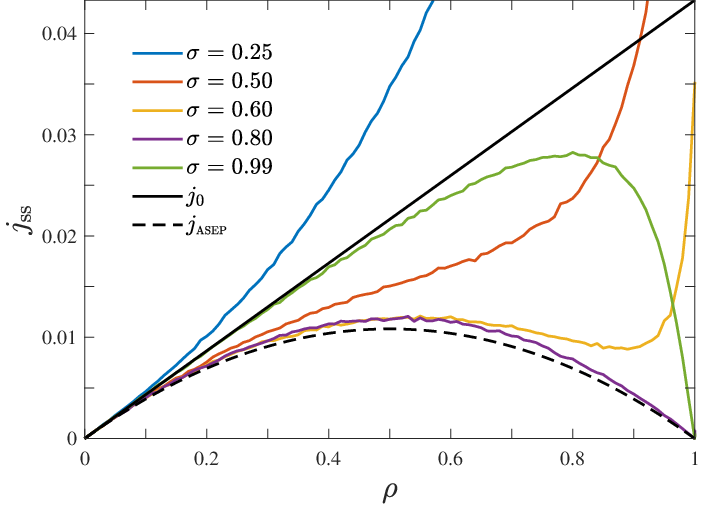
Four representative shapes of current-density relations are shown in Fig. 1. In the low-density limit, all curves collapse to the linear behavior with the slope given by the velocity of a single (non-interacting) particle. This is given by Ambegaokar and Halperin 1969
| (37) |
where . Beyond the small- region, the shapes change strongly with the particle size . This complex behavior is caused by three competing collective effects:
(i) The barrier reduction effect leads to a current increase with . It appears in multi-occupied wells, where particles are pushing each other to regions of higher potential energy and thus decrease an effective barrier for a transition to neighboring wells. The effect is best visible for small causing currents to be larger than (solid black line in Fig. 1). Likewise, for small and moderate , the strong current increase at larger is due to the occurrence of double-occupied wells.
(ii) The blocking effect suppresses the current by reducing the number of transitions between neighboring wells. It occurs for larger particle sizes: an extended particle is more easily blocked by another one occupying the neighboring well (compared to smaller ). To contrast with the most extreme case of blocking, the parabolic current-density relations of a corresponding ASEP is shown as the dashed line in Fig. 1.
(iii) The exchange symmetry effect causes a deformation of the current-density relation towards the linear behavior if the particle size is close to , , i.e. a multiple integer of . In the commensurate case , the current of interacting particles becomes equal to that of noninteracting ones. This effect is a consequence of the general relation
| (38) |
that maps the stationary current in a system with particles of diameter and density to that with particles of diameter and density , where is the integer part of .
IV Impact of external periodic potential
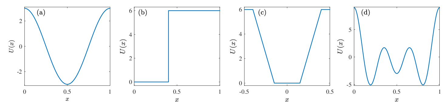
As discussed in the Introduction, we consider further external potentials, namely the Kronig-Penney, a piece-wise linear, and a triple-well potential. These potentials are plotted in Fig. 2(b)-(d) together with the cosine potential of our reference system in Fig. 2(a).

IV.1 Kronig-Penney potential
The Kronig-Penney potential has the form
| (39) |
where is width of the rectangular well, and the width of the rectangular barrier. We are interested in the current-density relation for different in the limit of large . Specifically, we take the same value as for the reference BASEP with cosine potential discussed in Sec. III. In particular, we aim to clarify, whether a current enhancement over that of noninteracting particles still occurs. As all particles dragged from one well to a neighboring one have to surmount the same barrier height now, it is not clear whether multiple occupation of wells lead to an effective barrier reduction. The blocking and exchange symmetry effect are expected to influence the current in an analogous manner.

Inserting the Kronig-Penney potential in Eq. (37) yields
| (40a) | ||||
| (40b) | ||||
| (40c) | ||||
for the single-particle velocity. This result is plotted in Fig. 3. As expected, approaches the mean drift velocity of a single particle in a flat potential in the limits (zero well width) and (zero barrier width). With increasing width of the wells (or of the barriers), rapidly decreases. Interestingly, Eq. (40c) implies the symmetry , that means the single-particle velocity remains unaltered if the barriers and wells are interchanged.
Current-density relations for hardcore interacting particles calculated from the SDA (cf. Sec. II.2) are shown in Fig. 4 for five different value of . For each , we plotted vs. for eight rod lengths analogous to our representation of current-density curves in Fig. 1. As can be seen from the graphs, the shapes of the current-density relation are qualitatively comparable to that in Fig. 1 for all , as well as their overall change with the diameter . This means that the interplay of the barrier reduction, blocking and exchange symmetry is still present. As expected, the overall strengths of the effects in modifying the current of noninteracting particles becomes weaker with decreasing ; for the current indeed approaches .
The barrier reduction, however, can no longer be associated with a decrease of an effective barrier height, when two or more particles occupy a potential well. For the Kronig-Potential in Eq. (39), all particles in a multiple-occupied well have zero energy and need to overcome . Nevertheless, we can attribute the enhancement of the current compared to that of noninteracting particles with a barrier reduction. To see this, we analyze the potential of mean force
| (41) |
for both the cosine and the Kronig-Penney potential, where the constant is chosen to give a potential minimum equal to zero. If considering driven Brownian motion of noninteracting particles in the potential , the current in the linear response limit would be equal to the many-particle current in the SDA. We therefore can interpret as an effective barrier in the many-particle system. In Fig. 5, we show for both the cosine and the Kronig-Penney potential. At the maximum of the cosine potential at , we find , that means the barrier height is reduced. In contrast, the barrier at the step of the Kronig-Penney potential equals ( in Fig. 5). However, a barrier reduction is now clearly seen in the plateau part of the barrier in the range . We thus can distinguish between two types of barrier reduction, namely the first type associated with a reduction of the barrier height and the second type associated with a lowering of the barrier plateau.

Generally, a single-well periodic potential can be characterized roughly by the widths of a valley and barrier part, and the flanks in between these parts. A simple representation is given by the piecewise linear potential
| (42) |
shown in Fig. 2(c), where , and are specifying the widths of the valley, barrier and flanks. We performed additional calculations in the SDA for this potential. For various fixed and , we always found current-density relations with a behavior similar to that found in Fig. 1 for the BASEP with cosine potential. This model may thus be viewed as representative for Brownian single-file transport through single-well periodic potentials with barriers much larger than the thermal energy.
Current-density relations with a different characteristics can, however, be obtained for multiple-well periodic potentials, as we discuss next.

IV.2 Triple-well potential
The triple-well potential shown in Fig. 2(d) is
| (43) |
where we choose here. For this potential, our calculations of based on the SDA show a very sensitive dependence on . We concentrate here on one particle diameter , where several local extrema occur, see Fig. 6. In this figure currents are shown up to a density (filling factor) , corresponding to a coverage of the system by the hard rods. If approaches its maximal value corresponding to a complete coverage, the numerical calculation of the equilibrium density profile from Eq. (19) becomes increasingly difficult. Hence, we refrained to show current data for due to a lack of sufficient numerical accuracy when calculating . It is important to state in this context that the current for is expected to approach that of noninteracting particles in a flat potential Lips et al. 2019, i.e. it should hold for [except for the singular point , where ]. This means that the current in Fig. 6 must steeply rise for , i.e. there must appear a further local minimum for . These arguments apply also to the currents shown in Figs. 1 and 4.
To explain the occurrence of the local extrema in Fig. 6, we resort to Eq. (15) with , i.e. the SDA. This equation can be interpreted by considering to be the “local conductivity” of a line segment . A serial connection of these segments implies that the “total conductivity” is given by the inverse of the sum of the inverse local conductivities, corresponding to a summation of the respective “local resistivities”. A stronger localization of around the minima of the potential leads to a smaller conductivity and hence a smaller current , while less localized density profiles lead to larger .
Using this picture, the occurrence of the first maximum in can be traced back to an increasing occurrence of double occupied wells for . In double-occupied wells, particle motion is more restricted, leading to a stronger particle localization at the two deeper minima at about and , see Fig. 2(d). Accordingly, starts to decrease with for [ in Fig. 6]. The decrease of continues up to a filling factor of about two [ in Fig. 6], above which more than two particles occupy a well on average. With a significant appearance of triple-occupied wells goes along first a stronger spreading of the density, as the minimum of the potential at becomes occupied in wells containing three particles. The spreading of the density causes to increase for . A counteracting effect, however, is a strong particle localization at all potential minima in neighboring triple-occupied wells, where the hardcore constraints force the particles to become strongly localized around the potential minima. For [ in Fig. 6], every second well is occupied by three particles on average which lets to decrease again with further increasing .
The more complex current-density relation in Fig. 6 leads to a richer variety of NESS phases in an open systems compared to the reference BASEP, which can exhibit up to five different phases Lips et al. 2018; Lips et al. 2019. To identify all possible NESS phases, we consider the particle exchange with two reservoirs L and R at the left and right end of an open system to be controlled by two parameters and . As discussed in connection with Eq. (1) in the Introduction, these control parameters can be considered as effective densities, or they can be associated with true reservoir densities for specific bulk-adapted couplings of the system to the reservoirs Dierl et al. 2013; Dierl et al. 2014.

Applying Eq. (1) with and to the current-density relation in Fig. 6 results in the diagram with seven different NESS phases I-VII shown in Fig. 7. The color coding shows the value of the bulk density , i.e. the order parameter of the phase transitions. Solid lines mark first order and dashed lines second order phase transitions, which is reflected in the smooth (continuous) or sudden (jump-like) changes of the color. The seven phases can be classified in two categories: boundary-matching phases, where is equal to either or , and extremal current phases, where is equal to one of the densities, where has a local extremum in Fig. 6. Specifically, the phases I and V are left-boundary matching phases with , the phases III and VII are right-boundary matching phases with , phase II is a maximal current phase with , phase VI a maximal current phase with , and phase IV a minimal current phase with . If one takes into account the existence of the further minimum for in the current-density relation (see discussion above), then even more phases are possible. These additional phases, however, must appear in the two stripes , i.e. in a very narrow range of one of the two control parameters (marked in black in Fig. 7).
V Impact of interactions other than hardcore exclusions
In this section, we investigate the impact of other particle interactions beyond hardcore exclusion for the cosine external potential in Eq. (36). This is done in two different settings. First, we investigate the repulsive Yukawa potential
| (44) |
between particles at distance for a fixed small amplitude and different decay length . Secondly, we combine this Yukawa interaction with hardcore interactions. For obtaining current-density relations, we here employ Brownian dynamics simulations. This is because an exact density functional is not available for the Yukawa interaction and the SDA with a precise determination of cannot be applied. For performing the Brownian dynamics simulations, we used a standard Euler integration scheme of the Langevin equations (2) with a time step . To deal with the hardcore interactions, the algorithm developed in Ref. Scala 2012 was applied.

Current-density relations for the Yukawa potential without additional hardcore interactions are shown in Fig. 8 for six different values of . These may be viewed to resemble effective particle diameters of hardcore interacting systems. For small , i.e. and in Fig. 8, shows an enhancement over that of noninteracting particles (solid black line) due to a prevailing barrier reduction effect similar to that in the reference BASEP for small . When enlarging , the current is reduced for small compared to that of noninteracting particles, while it rises strongly for large . Again this behavior is analogous to that in the reference BASEP for increasing . Because the (effective) blocking effect is not so strong for , the current-density curves do not approach the limiting as closely as for hardcore interactions. Nevertheless, one can say that the change of the current-density relation with varying is reflecting the interplay of a barrier reduction and blocking effect as in the reference BASEP.

However, one cannot find certain values, where the current-density relation equals that of noninteracting particles for all . The peculiar exchange symmetry effect in the BASEP for commensurate , , is caused by the invariance of the stochastic particle dynamics against a specific coordinate transformation containing Lips et al. 2018; Lips et al. 2019. Such coordinate transformation does not exist for the Yukawa potential.
For the Yukawa potential with additional hardcore interactions, we found changes of current-density curves caused by the barrier reduction and blocking effect as discussed above. But it is interesting to analyze now, whether the relation for commensurate and is approximately reflected in current-density relations for , where the exchange symmetry effect is no longer strictly valid. One may expect that the hardcore interacting system should be only weakly perturbed by the Yukawa potential if is of the order of the thermal energy and not too large compared to . This is indeed confirmed by simulation results for shown in Fig. 9. The data points for and lie almost directly on the curve up to the highest simulated density . With increasing , deviations from the linear behavior are seen, which become the more pronounced the larger . But even for , follows closely up to . We thus conclude that slight deviations from a perfect hardcore interaction, as they are always present in experiments, still allow an identification of the exchange symmetry effect.
VI Summary and Conclusions
To analyze how generic our previous findings are for the nonequilibrium physics of the BASEP in a sinusoidal potential, we have studied the driven Brownian motion of hardcore interacting particles for other external periodic potentials. Our calculations were carried out based on a small-driving approximation, which refers to the linear response under neglect of a period-averaged mean interaction force. If the external periodic potential exhibits a singe-well structure between barriers, i.e. if there is just one local minimum per period, our results provide evidence that the various characteristic shapes of bulk current-density relations for different particle sizes are always occurring. There are differences in the exact functional form and at which the shape type is changing. For all single-well periodic potentials it is the interplay of a barrier reduction, blocking and exchange symmetry effect that causes a particular shape type to appear. Even for a Kronig-Penney potential with alternating rectangular well and barrier parts, where the barrier reduction effect is not so obvious, we showed that an enhancement of the current over that of noninteracting particles occurs. For that potential this enhancement can be attributed to an effective reduction of the barrier plateau parts. The generic behavior of the bulk current-density relations implies that for single-well periodic potentials up to five different NESS phases appear in open BASEP systems coupled to particle reservoirs. This can be concluded by applying the extremal current principles Kolomeisky et al. 1998; Popkov and Schütz 1999.
More complex shape types of can occur in multiple-well periodic potentials. This was demonstrated for a particular triple-well potential, where our calculations yielded a current-density relation with two local maxima for a certain particle size. In that case the extremal current principles predict more than five different NESS in an open system. When neglecting a very narrow range of effective reservoir densities, which would be very difficult to realize by specific system-reservoir couplings in simulations or experiments, up to seven different NESS phases are possible. We point out that these results were obtained here for demonstration purposes. Systematic investigations of multiple-well external potentials should be performed in the future with a goal to reach a general classification similar as for the BASEP for single-well periodic potentials.
Current-density relations with several local maxima are particularly interesting in the case of “degenerate maxima”. i.e. when the current at the maxima has the same value. In such situations, coexisting NESS phases of maximal current can occur in a whole connected region of the space spanned by the parameters controlling the coupling to the environment Maass et al. 2018. Such states of coexisting extremal current phases have not yet been studied in detail in the literature. Preliminary results for driven lattice gases indicate that fluctuations of interfaces separating extremal current phases exhibit an anomalous scaling with time and system length 22 2 D. Locher, bachelor thesis (in German), Osnabrück University (2018); M. Bosi, D. Locher, and P. Maass, to be published.. This is in contrast to the already well-studied interface fluctuations between the low- and high-density phases in the ASEP, which at long times show a simple random-walk behavior.
We furthermore performed Brownian dynamics simulations of driven single-file diffusion through a cosine potential for a repulsive particle interaction other than hardcore exclusion. Specifically, we chose a Yukawa interaction with a small interaction amplitude equal to the thermal energy and studied the behavior for different decay lengths . Current-density relations for this system showed similar shapes as for the BASEP except for the effects implied by the exchange symmetry effect, which is absent for other interactions than hardcore. The change of shapes is solely determined by the interplay of a barrier reduction and effective blocking effect. If the hardcore interaction and the weak Yukawa interaction are combined, the consequences of the exchange symmetry effect can be still seen for particle sizes commensurate with the wavelength of the cosine potential. The current follows closely that of noninteracting particles up to high densities even for large . This means that deviations from a perfect hardcore interaction in experiments should still allow one to verify the exchange symmetry.
Acknowledgements.
Financial support by the Czech Science Foundation (Project No. 20-24748J) and the Deutsche Forschungsgemeinschaft (Project No. 397157593) is gratefully acknowledged. We sincerely thank the members of the DFG Research Unit FOR 2692 for fruitful discussions. *Appendix A Example for connection of ASEP to quantum spin chain
Let denote the probability of configurations of occupation numbers in a single-species fermionic lattice gas at time . Its time evolution is described by the master equation
| (45) |
where is the transition rate from configuration to (for , otherwise ), and . This master equation corresponds to the occupation number representation of a Schrödinger equation
| (46) |
in imaginary time Gwa and Spohn 1992; Sandow and Trimper 1993.
For the ASEP with periodic boundary conditions (, ), the transitions rates can be written as
| (47) |
where denotes the configuration with the occupation numbers at sites and interchanged, i.e., for , , and . Accordingly, the matrix elements are
| (48) |
Because for creation and annihilation operators and of a particle at site , the matrix elements in Eq. (48) are equal to that of the Hamiltonian
| (49) |
of spinless fermions, which for is non-Hermitian. In a representation by Pauli matrices, one can write , , , giving
| (50) |
The periodic boundary conditions imply and .
A transformed with (non-singular) operator has the same spectrum as , where eigenstates and of and to the same eigenvalue are related by . Such transformation can be used to symmetrize the non-Hermitian part in Eq. (50) by choosing with some constant , because Henkel and Schütz 1994. With and , the symmetrization is achieved by requiring , i.e. by setting . The transformed Hamiltonian is that of a quantum chain,
| (51) |
with , but now non-Hermitian boundary conditions , i.e. and .
References
- Derrida (1998) B. Derrida, Phys. Rep. 301, 65 (1998).
- Schütz (2001) G. M. Schütz, in Phase Transitions and Critical Phenomena, Vol. 19, edited by C. Domb and J. Lebowitz (Academic Press, London, 2001) pp. 1–251.
- Gwa and Spohn (1992) L.-H. Gwa and H. Spohn, Phys. Rev. A 46, 844 (1992).
- Sandow and Trimper (1993) S. Sandow and S. Trimper, Europhys. Lett. (EPL) 21, 799 (1993).
- Sandow (1994) S. Sandow, Phys. Rev. E 50, 2660 (1994).
- Henkel and Schütz (1994) M. Henkel and G. Schütz, Physica A 206, 187 (1994).
- Blythe and Evans (2007) R. A. Blythe and M. R. Evans, J. Phys. A Math. Theor. 40, R333 (2007).
- Krebs and Sandow (1997) K. Krebs and S. Sandow, J. Phys. A: Math. Gen. 30, 3165 (1997).
- Derrida and Lebowitz (1998) B. Derrida and J. L. Lebowitz, Phys. Rev. Lett. 80, 209 (1998).
- Derrida et al. (2002) B. Derrida, J. L. Lebowitz, and E. R. Speer, Phys. Rev. Lett. 89, 030601 (2002).
- Krapivsky et al. (2014) P. L. Krapivsky, K. Mallick, and T. Sadhu, Phys. Rev. Lett. 113, 078101 (2014).
- Bertini et al. (2015) L. Bertini, A. De Sole, D. Gabrielli, G. Jona-Lasinio, and C. Landim, Rev. Mod. Phys. 87, 593 (2015).
- Touchette (2009) H. Touchette, Phys. Rep. 478, 1 (2009).
- Bertini et al. (2005) L. Bertini, A. De Sole, D. Gabrielli, G. Jona-Lasinio, and C. Landim, Phys. Rev. Lett. 94, 030601 (2005).
- Bodineau and Derrida (2005) T. Bodineau and B. Derrida, Phys. Rev. E 72, 066110 (2005).
- Appert-Rolland et al. (2008) C. Appert-Rolland, B. Derrida, V. Lecomte, and F. van Wijland, Phys. Rev. E 78, 021122 (2008).
- Baek et al. (2017) Y. Baek, Y. Kafri, and V. Lecomte, Phys. Rev. Lett. 118, 030604 (2017).
- Bodineau and Derrida (2004) T. Bodineau and B. Derrida, Phys. Rev. Lett. 92, 180601 (2004).
- Schütz (1997) G. M. Schütz, J. Stat. Phys. 88, 427 (1997).
- Tracy and Widom (2008a) C. A. Tracy and H. Widom, Commun. Math. Phys. 279, 815 (2008a).
- Tracy and Widom (2008b) C. A. Tracy and H. Widom, J. Stat. Phys. 132, 291 (2008b).
- Tracy and Widom (2009) C. A. Tracy and H. Widom, Commun. Math. Phys. 290, 129 (2009).
- Johansson (2000) K. Johansson, Commun. Math. Phys. 209, 437 (2000).
- Kardar et al. (1986) M. Kardar, G. Parisi, and Y.-C. Zhang, Phys. Rev. Lett. 56, 889 (1986).
- Krug (1991) J. Krug, Phys. Rev. Lett. 67, 1882 (1991).
- Schütz and Domany (1993) G. Schütz and E. Domany, J. Stat. Phys. 72, 277 (1993).
- Kolomeisky et al. (1998) A. B. Kolomeisky, G. M. Schütz, E. B. Kolomeisky, and J. P. Straley, J. Phys. A: Math. Gen. 31, 6911 (1998).
- Brzank and Schütz (2007) A. Brzank and G. M. Schütz, J. Stat. Mech. Theor. Exp. 2007, P08028 (2007).
- Popkov and Schütz (1999) V. Popkov and G. M. Schütz, Europhys. Lett. 48, 257 (1999).
- Hager et al. (2001) J. S. Hager, J. Krug, V. Popkov, and G. M. Schütz, Phys. Rev. E 63, 056110 (2001).
- Antal and Schütz (2000) T. Antal and G. M. Schütz, Phys. Rev. E 62, 83 (2000).
- Dierl et al. (2012) M. Dierl, P. Maass, and M. Einax, Phys. Rev. Lett. 108, 060603 (2012).
- Dierl et al. (2013) M. Dierl, M. Einax, and P. Maass, Phys. Rev. E 87, 062126 (2013).
- Dierl et al. (2014) M. Dierl, W. Dieterich, M. Einax, and P. Maass, Phys. Rev. Lett. 112, 150601 (2014).
- Evans (1996) M. R. Evans, EPL 36, 13 (1996).
- Concannon and Blythe (2014) R. J. Concannon and R. A. Blythe, Phys. Rev. Lett. 112, 050603 (2014).
- Popkov and Salerno (2004) V. Popkov and M. Salerno, Phys. Rev. E 69, 046103 (2004).
- Popkov et al. (2015) V. Popkov, A. Schadschneider, J. Schmidt, and G. M. Schütz, PNAS 112, 12645 (2015).
- Prähofer and Spohn (2004) M. Prähofer and H. Spohn, J. Stat. Phys. 115, 255 (2004).
- Chen et al. (2018) Z. Chen, J. de Gier, I. Hiki, and T. Sasamoto, Phys. Rev. Lett. 120, 240601 (2018).
- Schadschneider et al. (2010) A. Schadschneider, D. Chowdhury, and K. Nishinari, Stochastic Transport in Complex Systems: From Molecules to Vehicles, 3rd ed. (Elsevier Science, Amsterdam, 2010).
- Chou et al. (2011) T. Chou, K. Mallick, and R. K. P. Zia, Rep. Prog. Phys. 74, 116601 (2011).
- MacDonald et al. (1968) C. T. MacDonald, J. H. Gibbs, and A. C. Pipkin, Biopolymers 6, 1 (1968).
- Kolomeisky (2013) A. B. Kolomeisky, J. Phys.: Condens. Matter 25, 463101 (2013).
- Appert-Rolland et al. (2015) C. Appert-Rolland, M. Ebbinghaus, and L. Santen, Phys. Rep. 593, 1 (2015).
- Nishinari et al. (2005) K. Nishinari, Y. Okada, A. Schadschneider, and D. Chowdhury, Phys. Rev. Lett. 95, 118101 (2005).
- Appert-Rolland et al. (2011) C. Appert-Rolland, J. Cividini, and H. J. Hilhorst, J. Stat. Mech. Theor. Exp. 2011, P10014 (2011).
- Foulaadvand and Maass (2016) M. E. Foulaadvand and P. Maass, Phys. Rev. E 94, 012304 (2016).
- Hille (2001) B. Hille, Ionic Channels of Excitable Membranes, 3rd ed. (Sinauer Associates, Sunderland MA, 2001).
- Cheng and Bowers (2007) C.-Y. Cheng and C. R. Bowers, ChemPhysChem 8, 2077 (2007).
- Dvoyashkin et al. (2014) M. Dvoyashkin, H. Bhase, N. Mirnazari, S. Vasenkov, and C. R. Bowers, Anal. Chem. 86, 2200 (2014).
- Nitzan (2001) A. Nitzan, Annu. Rev. Phys. Chem. 52, 681 (2001).
- Berlin et al. (2001) Y. A. Berlin, A. L. Burin, and M. A. Ratner, J. Am. Chem. Soc. 123, 260 (2001).
- Risken (1985) H. Risken, The Fokker-Planck Equation: Methods of Solution and Applications (Springer-Verlag Berlin, 1985).
- Lips et al. (2018) D. Lips, A. Ryabov, and P. Maass, Phys. Rev. Lett. 121, 160601 (2018).
- Lips et al. (2019) D. Lips, A. Ryabov, and P. Maass, Phys. Rev. E 100, 052121 (2019).
- Arzola et al. (2017) A. V. Arzola, M. Villasante-Barahona, K. Volke-Sepúlveda, P. Jákl, and P. Zemánek, Phys. Rev. Lett. 118, 138002 (2017).
- Skaug et al. (2018) M. J. Skaug, C. Schwemmer, S. Fringes, C. D. Rawlings, and A. W. Knoll, Science 359, 1505 (2018).
- Schwemmer et al. (2018) C. Schwemmer, S. Fringes, U. Duerig, Y. K. Ryu, and A. W. Knoll, Phys. Rev. Lett. 121, 104102 (2018).
- Stoop et al. (2019) R. Stoop, A. Straube, and P. Tierno, Nano Lett. 19, 433 (2019).
- Misiunas and Keyser (2019) K. Misiunas and U. F. Keyser, Phys. Rev. Lett. 122, 214501 (2019).
- Straube and Tierno (2013) A. V. Straube and P. Tierno, EPL 103, 28001 (2013).
- Ryabov et al. (2019) A. Ryabov, D. Lips, and P. Maass, J. Phys. Chem. C 123, 5714 (2019).
- Jain et al. (2007) K. Jain, R. Marathe, A. Chaudhuri, and A. Dhar, Phys. Rev. Lett. 99, 190601 (2007).
- Slanina (2009a) F. Slanina, Phys. Rev. E 80, 061135 (2009a).
- Slanina (2009b) F. Slanina, J. Stat. Phys. 135, 935 (2009b).
- Chaudhuri and Dhar (2011) D. Chaudhuri and A. Dhar, EPL (Europhysics Letters) 94, 30006 (2011).
- Chaudhuri et al. (2015) D. Chaudhuri, A. Raju, and A. Dhar, Phys. Rev. E 91, 050103 (2015).
- (69) To implement the periodic boundary conditions, we assume an ordered initial configuration , and introduce two fictive particles with enslaved coordinates and , which implies .
- Percus (1976) J. K. Percus, J. Stat. Phys. 15, 505 (1976).
- Seifert (2012) U. Seifert, Rep. Prog. Phys. 75, 126001 (2012).
- Šiler et al. (2008) M. Šiler, T. Čižmár, A. Jonáš, and P. Zemánek, New J. Phys. 10, 113010 (2008).
- Di Leonardo et al. (2007) R. Di Leonardo, S. Keen, J. Leach, C. D. Saunter, G. D. Love, G. Ruocco, and M. J. Padgett, Phys. Rev. E 76, 061402 (2007).
- Curran et al. (2010) A. Curran, A. Yao, G. Gibson, R. Bowman, J. Cooper, and M. Padgett, J. Biophotonics 3, 244 (2010).
- Šiler et al. (2012) M. Šiler, T. Čižmár, and P. Zemánek, Appl. Phys. Lett. 100, 051103 (2012).
- Ambegaokar and Halperin (1969) V. Ambegaokar and B. I. Halperin, Phys. Rev. Lett. 22, 1364 (1969).
- Scala (2012) A. Scala, Phys. Rev. E 86, 026709 (2012).
- Maass et al. (2018) P. Maass, M. Dierl, and M. Wolff, “On Phase Transitions in Biased Diffusion of Interacting Particles,” (Springer International Publishing, Cham, 2018) Chap. 9, pp. 147–168.
- (79) D. Locher, bachelor thesis (in German), Osnabrück University (2018); M. Bosi, D. Locher, and P. Maass, to be published.