Phase diagrams of interacting spreading dynamics in complex networks

Liming Pan Affiliation: School of Computer Science and Technology, Nanjing Normal University, Nanjing, Jiangsu, 210023, China Affiliation: Complex Lab, School of Computer Science and Engineering, University of Electronic Science and Technology of China, Chengdu, 611731, China Dan Yang Affiliation: Complex Lab, School of Computer Science and Engineering, University of Electronic Science and Technology of China, Chengdu, 611731, China Wei Wang Email: wwzqbx@hotmail.com Affiliation: Cybersecurity Research Institute, Sichuan University, Chengdu 610065, China Affiliation: Complex Lab, School of Computer Science and Engineering, University of Electronic Science and Technology of China, Chengdu, 611731, China Shimin Cai Affiliation: Complex Lab, School of Computer Science and Engineering, University of Electronic Science and Technology of China, Chengdu, 611731, China Affiliation: Institute of Fundamental and Frontier Sciences, University of Electronic Science and Technology of China, Chengdu 610054, China Affiliation: Big Data Research Center, University of Electronic Science and Technology of China, Chengdu 610054, China Tao Zhou Affiliation: Complex Lab, School of Computer Science and Engineering, University of Electronic Science and Technology of China, Chengdu, 611731, China Affiliation: Institute of Fundamental and Frontier Sciences, University of Electronic Science and Technology of China, Chengdu 610054, China Affiliation: Big Data Research Center, University of Electronic Science and Technology of China, Chengdu 610054, China Ying-Cheng Lai Affiliation: School of Electrical, Computer and Energy Engineering, Arizona State University, Tempe, AZ 85287, USA

August 11, 2026

Abstract

Epidemic spreading processes in the real world can interact with each other in a cooperative, competitive, or asymmetric way, requiring a description based on coevolution dynamics. Rich phenomena such as discontinuous outbreak transitions and hystereses can arise, but a full picture of these behaviors in the parameter space is lacking. We develop a theory for interacting spreading dynamics on complex networks through spectral dimension reduction. In particular, we derive from the microscopic quenched mean-field equations a two-dimensional system in terms of the macroscopic variables, which enables a full phase diagram to be determined analytically. The diagram predicts critical phenomena that were known previously but only numerically, such as the interplay between discontinuous transition and hysteresis as well as the emergence and role of tricritical points.

I Introduction

Spreading dynamics of diseases, behaviors and information in nature and human society are rarely independent processes but interact with each other in a complex way. Weakened immunity to other viruses due to HIV infection Ferguson et al. 2003; Abu-Raddad et al. 2006 and suppression of spreading due to disease-related information exchange on the social media Funk et al. 2009 are known examples. To better understand, predict, and control spreading on networks, coevolution of epidemics must be taken into account. In network science, there has been continuous interest in developing interacting epidemic models Gog and Grenfell 2002; Ferguson et al. 2003; Abu-Raddad et al. 2006; Eames and Keeling 2006a; Berkman et al. 2014; Sanz et al. 2014; Pastor-Satorras et al. 2015; de Arruda et al. 2018; Wang et al. 2019; Soriano-Paños et al. 2019; Eames and Keeling 2006b; Danziger et al. 2019; Soriano-Paños et al. 2019, which can generate surprising behaviors that cannot be predicted by any single-virus epidemic model. For example, spreading of one epidemic can facilitate that of another, leading to a first-order or explosive transition in the outbreak with significant real-world implications Cai et al. 2015. Many factors can affect the critical behaviors of interacting spreading dynamics, such as self-evolution of each epidemic Funk et al. 2009; Noh and Park 2005, interaction between two epidemics Granell et al. 2013; Wang et al. 2014, and network structure Hébert-Dufresne and Althouse 2015; Chen 2019.

By now, spreading dynamics of a single epidemic on complex networks have been well studied Castellano et al. 2009; Pastor-Satorras et al. 2015; Dorogovtsev et al. 2008; Kiss et al. 2017. For interacting spreading dynamics, the special case of well-mixed populations has been treated Abu-Raddad et al. 2008; Zarei et al. 2019. A study based on the quenched mean field for two competing pathogens Prakash et al. 2012a showed that, when simultaneous infection by the two pathogens is not possible (full mutual exclusion), the phase diagram is independent of the spectral radius of the network. There were also theories based on percolation Newman 2005, annealed mean field Chen et al. 2013 and pair approximations Hébert-Dufresne and Althouse 2015 to study the effect of network structure on interacting spreading, leading to a qualitative understanding of critical phenomena. There are difficulties with these theories. For example, the annealed mean-field theory takes into account only the nodal degrees and is not applicable to quenched networks (especially networks with a high clustering coefficient and modularity). For such networks, quenched mean-field theories Sahneh and Scoglio 2014 such as those based on Markov chains Granell et al. 2014 and the N-intertwined method Van Mieghem 2011 is needed. A deficiency of such a theory is that it uses a large number of nonlinear differential equations, with two difficulties: (a) high computational overload for large networks and (b) lack of any analytic insights. Such a theory, due to its heavy reliance on numerics, can lead to inconsistent or even contradicting predictions Achlioptas et al. 2009; da Costa et al. 2010. To our knowledge, a general analytic theory capable of providing a more complete understanding of interacting spreading dynamics is lacking.

In this paper, we develop an analytic theory for interacting spreading dynamics on complex networks through the approach of dimension reduction for complex networks Gao et al. 2016; Laurence et al. 2019; Jiang et al. 2018. From the quenched mean-field equations, we derive a two-dimensional (2D) system that is capable of analytically yielding the full Phase diagrams underlying interacting spreading dynamics on any complex network, from which the conditions for various phase transitions can be derived. The analytic model predicts critical phenomena that were previously known numerically, such as the interplay between discontinuous outbreak transitions and hystereses as well as the emergence of tricritical points, providing a solid theoretical foundation for understanding interacting spreading dynamics and articulating optimal control strategies.

II Model, method of spectral dimension reduction, and reduced model

II.1 Model

We consider the susceptible-infected-susceptible (SIS) model of interacting spreading dynamics on complex networks. In the classic SIS model, a single epidemic spreads in the network and a node can be either in the susceptible or in the infected state. Susceptible nodes are infected by their infected neighbors at rate $\lambda$ and infected nodes recover at rate $\gamma$ . For interacting SIS dynamics, two epidemics, say $1$ and $2$ , spread simultaneously and interact with each other. Each node infected by $a\in\{1,2\}$ transmits the infection to neighbors that are susceptible for both epidemics with probability $\lambda_{a}$ . If a neighbor is susceptible for $a$ but infected by the other epidemic, the infection will be transmitted with rate $\lambda^{\dagger}_{a}$ . All the nodes infected by $a$ recover to being susceptible with rate $\gamma_{a}$ . Without loss of generality, we set $\gamma_{a}=1$ for both $a\in\{1,2\}$ . In general, the nature of the interacting SIS dynamics depends on the interplay between the rates $\lambda_{a}$ and $\lambda_{a}^{\dagger}$ . In particular, for $\lambda_{a}^{\dagger}>\lambda_{a}$ , the two epidemics tend to facilitate each other, leading to cooperative SIS dynamics, whereas if $\lambda_{a}^{\dagger}<\lambda_{a}$ , infection with one epidemic will suppress infection with the other, giving rise to competitive SIS dynamics. For $\lambda_{a}^{\dagger}>\lambda_{a}$ but $\lambda_{b}^{\dagger}<\lambda_{b}$ for $a,b\in\{1,2\}$ with $\ b\neq a$ , the interactions are asymmetric.

II.2 Spectral dimension reduction

The interacting SIS model represents a paradigm to study rich dynamical behaviors such as first-order outbreak transitions and hystereses Chen et al. 2017. The foundation of our study of this model is the quenched mean-field theory (QMF) Wang et al. 2003. While in QMF the dynamical correlations among the neighbors are assumed to be negligible, the theory has been demonstrated to generate reliable prediction of the phase transitions Boguná et al. 2013. Since our goal is to analytically map out the complete phase diagram, using the QMF suffices. Let $p_{a,i}$ be the probability that node $i\in\{1,\cdots,N\}$ is infected by $a\in\{1,2\}$ at time $t$ . In the first-order mean-field analysis Sahneh and Scoglio 2014, the evolution of $p_{a,i}$ on a network with adjacency matrix $G$ is governed by

\begin{split}\frac{dp_{a,i}}{dt}=&-p_{a,i}+\lambda_{a}^{\dagger}\left(1-p_{a,i}\right)p_{b,i}\sum_{j}G_{ij}p_{a,j}\\ &+\lambda_{a}\left(1-p_{a,i}\right)\left(1-p_{b,i}\right)\sum_{j}G_{ij}p_{a,j}\end{split}

(1)

for $a\in\{1,2\}$ and $i\in\{1,\cdots,N\}$ . The first term on the right side of Eqs. (1) is the rate of recovery from epidemic $a$ for node $i$ , while the second (third) term corresponds to the rate of infection for epidemic $a$ with (without) $i$ already infected by $b\neq a$ . For a network of size $N$ , the number of equations in (1) is $2N$ . To derive an analytic model, we exploit the technique of spectral dimension reduction (SDR) Laurence et al. 2019 to arrive at an equivalent description of the original system in terms of two macroscopic observables - one for each epidemic. In particular, let $\alpha$ be a vector with nonnegative entries and normalized as $\sum_{i}\alpha_{i}=1$ . The entries of $\alpha$ represent the nodal weights. We define linear observables as $\psi_{a}=\alpha^{T}p_{a}$ for $a\in\{1,2\}$ . Since the entries of $\alpha$ are summed to unity, $\psi_{a}$ is a weighted average. The evolution of $\psi_{a}$ is determined by the equation

\frac{d\psi_{a}}{dt}=\sum_{i=1}^{N}\alpha_{i}\frac{dp_{a,i}}{dt}.

(2)

Applying the SDR method, we have that the right-hand side of Eq. (2) can be written in terms of the macroscopic observables $\psi_{a}$ only.

II.3 Reduced model

We apply the SDR method to Eq. (2). Microscopic variables $p_{a,i}$ fluctuate about the macroscopic observables $\psi_{a}$ , which can be decomposed as

\begin{split}&p_{a,i}=\rho_{a}\psi_{a}+\delta p_{a,i},\\ &p_{b,i}=\mu_{a}\psi_{b}+\delta p_{b,i},\\ &p_{a,j}=\nu_{a}\psi_{a}+\delta p_{a,j},\end{split}

(3)

where $\rho_{a}$ , $\mu_{a}$ , and $\nu_{a}$ are parameters to be determined, and $\delta p_{a,i}$ , $\delta p_{b,i}$ , and $\delta p_{a,j}$ are correction terms. Substituting Eqs. (1) and Eqs. (3) into Eqs. (2) gives

\begin{split}\frac{d\psi_{a}}{dt}=&-\psi_{a}+\lambda^{\dagger}_{a}\hat{\alpha}\mu_{a}\nu_{a}\left(1-\rho_{a}\psi_{a}\right)\psi_{b}\psi_{a}\\ &+\lambda_{a}\hat{\alpha}\nu_{a}\left(1-\rho_{a}\psi_{a}\right)(1-\mu_{a}\psi_{b})\psi_{a}+R_{a},\end{split}

(4)

where $\hat{\alpha}=\sum_{i,j}\alpha_{i}G_{ij}$ and $R_{a}$ is the remainder term that can be decomposed as

R_{a}=R_{a,1}+R_{a,2}+R_{a,3},

(5)

with $R_{a,1}$ , $R_{a,2}$ and $R_{a,3}$ containing the first-, second- and third-order terms in the corrections $\{\delta p_{a,i}\}$ , respectively. Let $K$ be the diagonal matrix with $K_{ii}$ being the degree of node $i$ , the first-order correction $R_{a,1}$ is given by

\begin{split}&R_{a,1}=\left[\left(\lambda_{a}-\lambda_{a}^{\dagger}\right)\mu_{a}\nu_{a}\psi_{b}\psi_{a}-\lambda_{a}\nu_{a}\psi_{a}\right]\alpha^{T}K\delta p_{a}\\ &+\left(\lambda_{a}^{\dagger}-\lambda_{a}\right)\nu_{a}\left(1-\rho_{a}\psi_{a}\right)\psi_{a}\alpha^{T}K\delta p_{b}\\ &+\left(1-\rho_{a}\psi_{a}\right)(\lambda_{a}^{\dagger}\mu_{a}\psi_{b}+\lambda_{a}-\lambda_{a}\mu_{a}\psi_{b})\alpha^{T}G\delta p_{a},\end{split}

(6)

where $\delta p_{a}$ is a vector with $\delta p_{a,i}$ in the $i$ th entry and $\delta p_{b}$ is defined analogously. The second-order remainder term is

\begin{split}&R_{a,2}=\left(\lambda_{a}^{\dagger}-\lambda_{a}\right)\left(1-\rho_{a}\psi_{a}\right)\sum_{i=1}^{N}\sum_{j=1}^{N}G_{ij}\alpha_{i}\delta p_{b,i}\delta p_{a,j}\\ &+\left[\left(\lambda_{a}-\lambda_{a}^{\dagger}\right)\mu_{a}\psi_{b}-\lambda_{a}\right]\sum_{i=1}^{N}\sum_{j=1}^{N}G_{ij}\alpha_{i}\delta p_{a,i}\delta p_{a,j}\\ &+\left(\lambda_{a}-\lambda_{a}^{\dagger}\right)\nu_{a}\psi_{a}\sum_{i=1}^{N}\sum_{j=1}^{N}G_{ij}\alpha_{i}\delta p_{a,i}\delta p_{b,i}\end{split}

(7)

and the third-order remainder term is

R_{a,3}=\left(\lambda_{a}-\lambda_{a}^{\dagger}\right)\sum_{i=1}^{N}\sum_{j=1}^{N}G_{ij}\alpha_{i}\delta p_{a,i}\delta p_{b,i}\delta p_{a,j}.

(8)

From Eq. (6), the dominant remainder term $R_{a,1}$ vanishes if the following equations hold

\begin{split}&\alpha^{T}Kp_{a}=\hat{\alpha}\rho_{a}\psi_{a},\\ &\alpha^{T}Kp_{b}=\hat{\alpha}\mu_{a}\psi_{b},\\ &\alpha^{T}Gp_{a}=\hat{\alpha}\nu_{a}\psi_{a},\end{split}

(9)

where $p_{a}$ is a vector with $p_{a,i}$ in the $i$ th entry and $p_{b}$ is defined similarly.

In general, the equations cannot be satisfied simultaneously. An application of the SDR method in Ref. Laurence et al. 2019 advocates choosing $\alpha$ as the eigenvector associated with the leading eigenvalue $\omega$ of $G$ . For connected undirected networks, the eigenvector associated with the leading eigenvalue $\omega$ of $G$ has positive entries. The third equation in Eqs. (9) implies $\omega\psi_{a}=\hat{\alpha}\nu_{a}\psi_{a}$ and, hence, $\omega=\nu_{a}\hat{\alpha}$ . Using the definition $\hat{\alpha}=\mathbf{1}^{T}G\alpha=\omega$ , we have $\nu_{a}=1$ . The remaining two parameters, $\rho_{a}$ and $\mu_{b}$ , are chosen such that the first two equations in Eqs. (9) are satisfied. The quantities $\rho_{a}$ and $\mu_{b}$ can be chosen by minimizing the following squared vector norm

\begin{split}\rho_{a}^{*}=\mu_{a}^{*}=\underset{x}{\mathrm{argmin}}\|K\alpha-x\hat{\alpha}\alpha\|_{2}^{2},\end{split}

which yields

\mu\mathop{:}=\frac{1}{\omega}\frac{\alpha^{T}K\alpha}{\alpha^{T}\alpha}=\rho_{a}^{*}=\mu_{a}^{*}.

(10)

A justification of the parameter choices was given in Ref. Laurence et al. 2019. With the parameters chosen, $R_{a,1}$ can be made as small as possible and can be neglected, so can the higher order terms $R_{a,2}$ and $R_{a,3}$ . Substituting the values of $\rho_{a}$ , $\mu_{a}$ and $\nu_{a}$ into Eqs. (4), we get

\begin{split}\frac{d\psi_{a}}{dt}=&-\psi_{a}+\lambda^{\dagger}_{a}\omega\mu\left(1-\mu\psi_{a}\right)\psi_{b}\psi_{a}\\ &+\lambda_{a}\omega\left(1-\mu\psi_{a}\right)(1-\mu\psi_{b})\psi_{a}+R_{a}.\end{split}

(11)

The first term on the right side of Eqs. (11) accounts for the rate of recovery and the second (third) term represents the rate of infection for epidemic $a$ with (without) being infected by $b\neq a$ . The quantity $R_{a}$ in Eqs. (11) characterizes the fluctuations of the microscopic observables $p_{a,i}$ about the macroscopic observables $\psi_{a}$ , which is small in comparison to other terms on the right side of Eqs. (11) due to $\alpha$ ’s being the leading eigenvector. Since, for finding the phase diagram, it is necessary to analyze the mean-field equations that depend on the macroscopic observables $\psi_{a}$ only, it is justified to drop $R_{a}$ from the analysis. As we will verify numerically, this approximation will not affect the accuracy of the phase diagram as the resulting errors near the phase boundaries are quite insignificant.

In Eqs. (1), the order parameters are $\langle p_{a,i}\rangle$ for $a\in\{1,2\}$ , where $\langle\cdot\rangle$ is the unweighted average over the nodes. In Eqs. (11), the order parameters can be chosen to be $\psi_{a}=\alpha^{T}p_{a}$ , a weighted average over the nodes. Since $\alpha$ is the eigenvector associated with the leading eigenvalue of $G$ , its entries are strictly positive. As a result, $\psi_{a}=0$ ( $\psi_{a}>0$ ) implies $\langle p_{a,i}\rangle=0$ ( $\langle p_{a,i}\rangle>0$ ). When crossing a phase boundary, at least one of $\psi_{a}$ for $a\in\{1,2\}$ becomes either zero or nonzero, guaranteeing that the corresponding $\langle p_{a,i}\rangle$ becomes either zero or nonzero, respectively. We have that $\langle p_{a,i}\rangle$ and $\psi_{a}$ give the same phase diagram, which can be obtained analytically through the 2D mean-field system.

III Main result: phase diagram of reduced system

The reduced mean-field equations are amenable to analytic treatment. As the derivations are lengthy, we provide a brief sketch of the results from analyzing the reduced system.

The analyses of the 2D mean-field system are performed in the following steps. First, for each point in the parameter space $(\lambda_{1}$ , $\lambda_{1}^{\dagger},\lambda_{2}$ , $\lambda_{2}^{\dagger})$ , we determine the equilibrium points of Eqs. (11) (Sec. III.1) and their stability (Sec. III.2). The the equilibrium points have to further satisfy the probability constraint $1\leq\psi_{a}\leq 1$ to be physical meaningful. A detailed analysis of the stability and probability constraints of the equilibrium points leads to the following functions of $\lambda_{a}$ and $\lambda_{a}^{\dagger}$ :

\begin{split}s_{a,0}=&\lambda_{b}+\lambda^{\dagger}_{a}-\lambda_{a}-\omega\lambda_{b}\lambda^{\dagger}_{a},\\ s_{a,1}=&\lambda^{\dagger}_{b}-\lambda_{b}-\lambda^{\dagger}_{a}+\lambda_{a}+2\omega\lambda_{b}\lambda^{\dagger}_{a}-\omega\lambda^{\dagger}_{a}\lambda^{\dagger}_{b},\\ s_{a,2}=&\lambda^{\dagger}_{b}-\lambda_{b},\ s_{a,3}=\lambda_{a}-\omega^{-1},\\ s_{\Delta}=&(\lambda^{\dagger}_{1}-\lambda_{1}+\lambda^{\dagger}_{2}-\lambda_{2}-\omega\lambda^{\dagger}_{1}\lambda^{\dagger}_{2})^{2},\\ &-4(\lambda^{\dagger}_{1}-\lambda_{1})(\lambda^{\dagger}_{2}-\lambda_{2}).\end{split}

(12)

for $a,b\in\{1,2\}$ and $a\neq b$ . Whether an equilibrium point is physical or stable is determined by the signs of these functions.

Calculating the equilibrium points (Sec. III.1) and analyzing their stability (Sec. III.2) enable us to obtain the full phase diagram of the reduced system and the equations for the phase boundaries (Sec. III.3). Based on the numbers of stable and unstable equilibrium points as well as the relationships among them, we can divide the parameter space into distinct regions, where a boundary crossing between two neighboring regions gives rise to a phase transition. A region either can have a unique stable equilibrium point or can have two stable equilibrium points with one unstable point in between, where crossing the latter will result in a hysteresis. We discuss the types of phase transitions crossing the various boundaries and study the interplay between the transitions and the phenomenon of hysteresis (Sec. III.4). Finally, we derive the conditions under which a hysteresis can arise (Sec. III.5).

The analytical results of the full phase diagram are summarized and discussed in Sec. III.6. Readers who are not interested in the technical details of analyzing the 2D mean-field system can skip Secs. III.1 to III.5 and check Sec. III.6 for the results. For convenience, for the rest of the paper, we use the convention that, if variables indexed by $a,b\in\{1,2\}$ (e.g., $\psi_{a}$ and $\psi_{b}$ ) appear together in an equation or an inequality, the assumption is $a\neq b$ .

III.1 Equilibrium points of the reduced system

The equilibrium points are obtained by setting the right side of Eqs. (11) to zero:

\begin{split}&-\psi_{a}+\lambda^{\dagger}_{a}\omega\mu\left(1-\mu\psi_{a}\right)\psi_{b}\psi_{a}\\ &+\lambda_{a}\omega\left(1-\mu\psi_{a}\right)(1-\mu\psi_{b})\psi_{a}=0\end{split}

(13)

for $a,b\in\{1,2\}$ and $a\neq b$ . Further, the physical solutions have to satisfy the probability constraints $0\leq\psi_{a}\leq 1$ . Because of the appearance of terms such as $\left(1-\mu\psi_{a}\right)$ in Eqs. (11), it is necessary to impose the physical condition $\left(1-\mu\psi_{a}\right)\leq 1$ . It can be proved that $\mu$ given by Eq. (10) satisfies $\mu\geq 1$ (see Appendix A for a proof), and it can also be verified that any point with $\psi_{1}=\mu^{-1}$ or $\psi_{2}=\mu^{-1}$ cannot be an equilibrium point. These, together the probability constraints, imply that all the equilibrium points must satisfy the inequality $0\leq\psi_{a}<\mu^{-1}$ for $a\in\{1,2\}$ .

We are now in a position to discuss the types of equilibrium points of the reduced mean-field equations.

(i) Epidemic free. The trivial solution $\left(\psi_{1},\psi_{2}\right)=(0,0)$ is always an equilibrium point.

(ii) Partial infection of epidemic $1$ . For $\psi_{1}\neq 0$ and $\psi_{2}=0$ , Eqs. (13) become

-1+\lambda_{1}\omega\left(1-\mu\psi_{1}\right)=0,

(14)

which gives

\psi_{1}=\frac{\lambda_{1}\omega-1}{\mu\lambda_{1}\omega}.

(15)

The solution further has to satisfy the probability constraint $0<\psi_{1}\leq\mu^{-1}$ . The first inequality $\psi_{1}>0$ is satisfied when $\lambda_{1}\omega>1$ , while the second inequality $\psi_{1}\leq\mu^{-1}$ always holds.

(iii) Partial infection of epidemic $2$ . Similar to case (ii), we have the equilibrium point:

\left(\psi_{1},\psi_{2}\right)=\left(0,\frac{\lambda_{2}\omega-1}{\mu\lambda_{2}\omega}\right).

(16)

(iv) Coexistence. If $\psi_{a}\neq 0$ for both $a\in\{1,2\}$ , Eqs. (13) become


	$\displaystyle\lambda^{\dagger}_{1}\omega\mu\left(1-\mu\psi_{1}\right)\psi_{2}+\lambda_{1}\omega\left(1-\mu\psi_{1}\right)(1-\mu\psi_{2})=1,$		(17a)
	$\displaystyle\lambda^{\dagger}_{2}\omega\mu\left(1-\mu\psi_{2}\right)\psi_{1}+\lambda_{2}\omega\left(1-\mu\psi_{2}\right)(1-\mu\psi_{1})=1.$		(17b)

Rearranging the second equation, we get

\psi_{2}=\mu^{-1}-\frac{1}{\left(\lambda^{\dagger}_{2}-\lambda_{2}\right)\mu^{2}\omega\psi_{1}+\lambda_{2}\mu\omega}.

(18)

Substituting this relation into Eq. (17a), we get an equation that depends on $\psi_{1}$ only. Similarly we can obtain the equation that determines $\psi_{2}$ . The two equations for $\psi_{1}$ and $\psi_{2}$ have the following symmetric form:

g_{a,2}\psi_{a}^{2}+g_{a,1}\psi_{a}+g_{a,0}=0

(19)

for $a\in\{1,2\}$ , where

\begin{split}g_{a,2}&=\omega^{2}\mu^{3}\lambda^{\dagger}_{a}\left(\lambda^{\dagger}_{b}-\lambda_{b}\right),\\ g_{a,1}&=\omega\mu^{2}\left(\lambda^{\dagger}_{b}-\lambda_{b}-\lambda^{\dagger}_{a}+\lambda_{a}+2\omega\lambda_{b}\lambda^{\dagger}_{a}-\omega\lambda^{\dagger}_{a}\lambda^{\dagger}_{b}\right),\\ g_{a,0}&=\omega\mu\left(\lambda_{b}+\lambda^{\dagger}_{a}-\lambda_{a}-\omega\lambda_{b}\lambda^{\dagger}_{a}\right)\end{split}

(20)

for $b\in\{1,2\}$ and $b\neq a$ .

If $\lambda_{a}^{\dagger}\neq\lambda_{a}$ holds for $a\in\{1,2\}$ , $g_{a,2}\neq 0$ and Eqs. (19) will be quadratic, leading to two solutions

\psi_{a}^{\pm}=\frac{-g_{a,1}\pm\sqrt{g_{a,1}^{2}-4g_{a,2}g_{a,0}}}{2g_{a,2}}.

(21)

The solutions for $a\in\{1,2\}$ are paired as

\left(\psi_{1},\psi_{2}\right)=\left(\psi_{1}^{+},\psi_{2}^{+}\right),\ \left(\psi_{1},\psi_{2}\right)=\left(\psi_{1}^{-},\psi_{2}^{-}\right).

(22)

If $\lambda_{a}^{\dagger}=\lambda_{a}$ for one or both $a\in\{1,2\}$ , we have

\psi_{a}=-\frac{g_{a,0}}{g_{a,1}}.

(23)

To discuss the probability constraints of the equilibrium points, we consider the following cases.

(iv.1) If $g_{a,2}=0$ for one of $a\in\{1,2\}$ , i.e., $\lambda_{b}^{\dagger}=\lambda_{b}$ , then there is a unique solution given by

\psi_{a}=\mu^{-1}-\frac{\lambda_{b}}{\mu\left(\lambda_{a}-\lambda_{a}^{\dagger}+\omega\lambda_{b}\lambda_{a}^{\dagger}\right)},\ \psi_{b}=\mu^{-1}-\frac{1}{\mu\omega\lambda_{b}}.

(24)

The probability constraints imply

\lambda_{a}-\lambda_{b}-\lambda_{a}^{\dagger}+\omega\lambda_{b}\lambda_{a}^{\dagger}>0,\ \omega\lambda_{b}>1.

(25)

Further, if we have $\lambda_{a}^{\dagger}=\lambda_{a}$ , the two epidemics will become independent of each other with the solution

\psi_{a}=\mu^{-1}-\frac{1}{\omega\mu\lambda_{a}},\ \psi_{b}=\mu^{-1}-\frac{1}{\omega\mu\lambda_{b}}.

(26)

(iv.2) Suppose $\lambda_{a}^{\dagger}>\lambda_{a}$ for both $a\in\{1,2\}$ . In this case there are two solutions, as shown in Eqs. (22).

Consider the solution

\left(\psi_{1},\psi_{2}\right)=\left(\psi_{1}^{+},\psi_{2}^{+}\right).

Firstly, it is necessary to have $g_{a,1}^{2}-4g_{a,2}g_{a,0}\geq 0$ for $a\in\{1,2\}$ to make the solutions real. Because of the condition $g_{a,2}>0$ , the probability constraints $0<\psi_{a}<\mu^{-1}$ imply

g_{a,1}<\sqrt{g_{a,1}^{2}-4g_{a,2}g_{a,0}}<2\mu^{-1}g_{a,2}+g_{a,1}

(27)

for $a\in\{1,2\}$ . The second inequality can be written as

\mu^{-2}g_{a,2}+\mu^{-1}g_{a,1}+g_{a,0}>0.

(28)

Substituting these into Eqs. (20), we have

g_{a,0}+\mu^{-1}g_{a,1}+\mu^{-2}g_{a,2}=\mu\omega\lambda_{b}^{\dagger}>0,

(29)

indicating that the second inequality always holds.

It remains to consider the first inequality in Eqs. (27). Suppose $g_{a,0}<0$ , then both the first and the inequality $g_{a,1}^{2}-4g_{a,2}g_{a,0}\geq 0$ hold. Otherwise, suppose $g_{a,0}>0$ , it is necessary to have $g_{a,1}<0$ and $g_{a,1}^{2}-4g_{a,2}g_{a,0}\geq 0$ .

Combining the discussions above, we have that $\left(\psi_{1}^{+},\psi_{2}^{+}\right)$ is a physical solution either for $g_{a,0}<0$ or for $g_{a,0}>0$ , $g_{a,1}<0$ , $g_{a,1}^{2}-4g_{a,2}g_{a,0}\geq 0$ for both $a\in\{1,2\}$ .

We now consider the solution $\left(\psi_{1},\psi_{2}\right)=\left(\psi_{1}^{-},\psi_{2}^{-}\right)$ . In order for the solution to be meaningful, it has to be guaranteed that $g_{a,1}^{2}-4g_{a,2}g_{a,0}\geq 0$ for $a\in\{1,2\}$ . The probability constraints give

g_{a,1}<-\sqrt{g_{a,1}^{2}-4g_{a,2}g_{a,0}}<2\mu^{-1}g_{a,2}+g_{a,1}.

(30)

The first inequality implies $g_{a,1}<0$ and $g_{a,0}>0$ . Consider the second inequality. If $2\mu^{-1}g_{a,2}+g_{a,1}>0$ , then the second inequality will be satisfied. Else if $2\mu^{-1}g_{a,2}+g_{a,1}\leq 0$ , the second inequality can be written as

\mu^{-2}g_{a,2}+\mu^{-1}g_{a,1}+g_{a,0}\leq 0.

(31)

Substituting these into Eqs. (20) we have

g_{a,0}+\mu^{-1}g_{a,1}+\mu^{-2}g_{a,2}=\mu\omega\lambda_{b}^{\dagger}>0,

(32)

which leads to a contradiction. It is thus necessary to have $2\mu^{-1}g_{a,2}+g_{a,1}\geq 0$ for $a\in\{1,2\}$ . In fact, the inequalities $g_{a,1}<0$ and $g_{a,0}>0$ are sufficient to guarantee the condition $2\mu^{-1}g_{a,2}+g_{a,1}\geq 0$ . For $g_{1,1}+g_{2,1}<0$ , we have

\lambda^{\dagger}_{1}+\lambda^{\dagger}_{2}-\omega\lambda^{\dagger}_{1}\lambda^{\dagger}_{2}<0.

(33)

We then have

\begin{split}2\mu^{-1}g_{1,2}+g_{1,1}=&\omega\mu^{2}\left(\lambda^{\dagger}_{2}-\lambda_{2}-\lambda^{\dagger}_{1}+\lambda_{1}+\omega\lambda^{\dagger}_{1}\lambda^{\dagger}_{2}\right)\\ >&\omega\mu^{2}\left(2\lambda^{\dagger}_{2}-\lambda_{2}+\lambda_{1}\right)>0.\end{split}

(34)

Similarly, we obtain $2\mu^{-1}g_{2,2}+g_{2,1}>0$ .

Combining the conditions discussed above, we have that the solution $\left(\psi_{1},\psi_{2}\right)=\left(\psi_{1}^{-},\psi_{2}^{-}\right)$ is physical for $g_{a,2}>0$ , $g_{a,1}<0$ , $g_{a,0}>0$ and $g_{a,1}^{2}-4g_{a,2}g_{a,0}>0$ for $a\in\{1,2\}$ . Comparing with the conditions for $\left(\psi_{1},\psi_{2}\right)=\left(\psi_{1}^{+},\psi_{2}^{+}\right)$ , we see that, for $g_{a,0}<0$ , only one physical solution is possible.

(iv.3) Suppose $\lambda_{a}^{\dagger}<\lambda_{a}$ for $a\in\{1,2\}$ and $\lambda_{b}^{\dagger}>\lambda_{b}$ for $b\in\{1,2\}$ and $b\neq a$ . We have $g_{a,2}>0$ and $g_{b,2}<0$ . Consider the solution $\left(\psi_{1},\psi_{2}\right)=\left(\psi_{1}^{+},\psi_{2}^{+}\right)$ . The probability constraints imply


		$\displaystyle g_{a,1}<\sqrt{g_{a,1}^{2}-4g_{a,2}g_{a,0}}<2\mu^{-1}g_{a,2}+g_{a,1},$		(35a)
		$\displaystyle g_{b,1}>\sqrt{g_{b,1}^{2}-4g_{b,2}g_{b,0}}>2\mu^{-1}g_{b,2}+g_{b,1}.$		(35b)

From Eq. (35a) we must have either $g_{a,0}<0$ or $g_{a,0}>0$ , $g_{a,1}<0$ , $g_{a,1}^{2}-4g_{a,2}g_{a,0}>0$ . The first inequality in Eq. (35b) implies $g_{b,1}>0$ and $g_{b,0}<0$ . Now consider the second inequality in Eq. (35b). For $2\mu^{-1}g_{b,2}+g_{b,1}\leq 0$ , the second inequality in Eq. (35b) holds. Otherwise if $2\mu^{-1}g_{b,2}+g_{b,1}>0$ , the second inequality implies

c_{b,0}+\mu^{-1}c_{b,1}+\mu^{-2}c_{b,2}>0

(36)

which always holds since the left side of the above inequality equals $\mu\omega\lambda_{a}^{\dagger}$ .

Recall that, from Eq. (35a), we can have either $g_{a,0}<0$ or $g_{a,0}>0$ , $g_{a,1}<0$ , $g_{a,1}^{2}-4g_{a,2}g_{a,0}>0$ . We can show that the latter case contradicts with the conditions $g_{b,1}>0$ and $g_{b,0}<0$ . In particular, from

g_{b,0}=\omega\mu\left(\lambda_{a}\left(1-\omega\lambda_{b}^{\dagger}\right)+\lambda_{b}^{\dagger}-\lambda_{b}\right)<0,

(37)

we have $1-\omega\lambda_{b}^{\dagger}<0$ and similarly

g_{a,0}=\omega\mu\left(\lambda_{b}\left(1-\omega\lambda_{a}^{\dagger}\right)+\lambda_{a}^{\dagger}-\lambda_{a}\right)>0,

(38)

implying $1-\omega\lambda_{a}^{\dagger}>0$ . Since

\begin{split}g_{a,1}&=\omega\mu^{2}\left(\lambda^{\dagger}_{b}-\lambda_{b}-\lambda^{\dagger}_{a}+\lambda_{a}+2\omega\lambda_{b}\lambda^{\dagger}_{a}-\omega\lambda^{\dagger}_{a}\lambda^{\dagger}_{b}\right)\\ &=\omega\mu^{2}\left(\left(\lambda_{b}^{\dagger}-\lambda_{b}\right)\left(1-\omega\lambda_{a}^{\dagger}\right)+\lambda_{a}-\lambda_{a}^{\dagger}\left(1-\omega\lambda_{b}\right)\right),\end{split}

(39)

then $g_{a,1}<0$ implies

\lambda_{a}-\lambda_{a}^{\dagger}\left(1-\omega\lambda_{b}\right)<0.

(40)

As a result, we have $\left(1-\omega\lambda_{b}\right)>\lambda_{a}/\lambda_{a}^{\dagger}>1$ and $\omega\lambda_{b}<0$ , leading to a contradiction.

Summarizing the above discussions about the equilibrium points, we have that $\left(\psi_{1},\psi_{2}\right)=\left(\psi_{1}^{+},\psi_{2}^{+}\right)$ is physical for $g_{a,0}<0$ , $g_{b,0}<0$ and $g_{b,1}>0$ . Note that $g_{b,1}>0$ is implied by the other two. Since

g_{b,1}+\mu g_{b,0}=\omega\mu^{2}\left(\lambda_{a}^{\dagger}+\omega\lambda_{b}^{\dagger}\left(\lambda_{a}-\lambda_{a}^{\dagger}\right)\right)>0,

(41)

we have that $g_{b,1}>0$ always holds given $g_{b,0}<0$ . Together, it is sufficient to have $g_{a,0}<0$ and $g_{b,0}<0$ .

We consider the solution $\left(\psi_{1},\psi_{2}\right)=\left(\psi_{1}^{-},\psi_{2}^{-}\right)$ . The probability constraints imply


		$\displaystyle g_{a,1}<-\sqrt{g_{a,1}^{2}-4g_{a,2}g_{a,0}}<2\mu^{-1}g_{a,2}+g_{a,1},$		(42a)
		$\displaystyle g_{b,1}>-\sqrt{g_{b,1}^{2}-4g_{b,2}g_{b,0}}>2\mu^{-1}g_{b,2}+g_{b,1}.$		(42b)

From Eq. (42b) we have $2\mu^{-1}g_{b,2}+g_{b,1}<0$ , giving

g_{b,0}+\mu^{-1}g_{b,1}+\mu^{-2}g_{b,2}<0.

(43)

which cannot hold since its left side equals $\mu\omega\lambda_{a}^{\dagger}$ . Thus, in this region, no physical solution of $\left(\psi_{1},\psi_{2}\right)=\left(\psi_{1}^{-},\psi_{2}^{-}\right)$ exists.

(iv.4) Suppose $\lambda_{a}^{\dagger}<\lambda_{a}$ for $a\in\{1,2\}$ , then $c_{a,2}<0$ . For the solution $\left(\psi_{1},\psi_{2}\right)=\left(\psi_{1}^{+},\psi_{2}^{+}\right)$ , we must have $g_{a,1}>0$ and $g_{a,0}<0$ for $a\in\{1,2\}$ . Similar to the discussions in the case (iv.3), we have that the sufficient condition for an equilibrium point is $g_{a,0}<0$ for $a\in\{1,2\}$ . The solution $\left(\psi_{1},\psi_{2}\right)=\left(\psi_{1}^{-},\psi_{2}^{-}\right)$ is nonphysical - see the discussion in (iv.3).

III.2 Stability analysis

The starting point to study the stability of the equilibrium points is the Jacobian matrix $J$ of the 2D mean-field system, whose entries are

\begin{split}J_{11}=&-1+\lambda^{\dagger}_{1}\omega\mu\left(1-2x\psi_{1}\right)\psi_{2}\\ &+\lambda_{1}\omega\left(1-2\mu\psi_{1}\right)(1-\mu\psi_{2}),\\ J_{12}=&\omega\mu\left(\lambda^{\dagger}_{1}-\lambda_{1}\right)\left(1-\mu\psi_{1}\right)\psi_{1},\\ J_{21}=&\omega\mu\left(\lambda^{\dagger}_{2}-\lambda_{2}\right)\left(1-\mu\psi_{2}\right)\psi_{2},\\ J_{22}=&-1+\lambda^{\dagger}_{2}\omega\mu\left(1-2\mu\psi_{2}\right)\psi_{1}\\ &+\lambda_{2}\omega\left(1-2\mu\psi_{2}\right)(1-\mu\psi_{1}).\end{split}

(44)

We analyze the stability of the different classes of equilibrium points as discussed in Sec. III.1.

(i) Epidemic free. For $\left(\psi_{1},\psi_{2}\right)=(0,0)$ , the Jacobian matrix is

J=\left({\begin{array}[]{cc}-1+\lambda_{1}\omega&0\\ 0&-1+\lambda_{2}\omega\end{array}}\right),

(45)

The equilibrium point is stable for $\lambda_{a}<\omega^{-1}$ for $a\in\{1,2\}$ .

(ii) Partial infection of epidemic $1$ . In this case, we have

\left(\psi_{1},\psi_{2}\right)=\left(\frac{\lambda_{1}\omega-1}{\mu\lambda_{1}\omega},0\right)

(46)

and $J_{21}=0$ , so the Jacobian is upper triangular, whose eigenvalues are simply the diagonal entries:

\begin{split}J_{1,1}&=1-\lambda_{1}\omega\\ J_{2,2}&=-1+\frac{\lambda_{2}}{\lambda_{1}}+\lambda_{2}^{\dagger}\frac{\lambda_{1}\omega-1}{\lambda_{1}}\end{split}

(47)

The equilibrium point is stable for $J_{1,1}<0$ and $J_{2,2}<0$ , i.e.,

\begin{split}&\lambda_{1}>\omega^{-1},\\ &\lambda_{2}-\lambda_{2}^{\dagger}-\lambda_{1}+\omega\lambda_{1}\lambda_{2}^{\dagger}<0.\end{split}

(48)

(iii) Partial infection of epidemic $2$ . For this type of equilibrium point, we have

\left(\psi_{1},\psi_{2}\right)=\left(0,\frac{\lambda_{2}\omega-1}{\mu\lambda_{2}\omega}\right).

(49)

It is stable under the following conditions:

\begin{split}&\lambda_{2}>\omega^{-1},\\ &\lambda_{1}-\lambda_{1}^{\dagger}-\lambda_{2}+\omega\lambda_{2}\lambda_{1}^{\dagger}<0.\end{split}

(50)

(iv) Coexistence. Suppose we have $\psi_{a}\neq 0$ for $a\in\{1,2\}$ . Substituting Eqs. (17) into Eqs. (44), the Jacobian matrix has entries

\begin{split}&J_{11}=\mu\psi_{1}/(\mu\psi_{1}-1),\\ &J_{12}=\omega\mu\left(\lambda^{\dagger}_{1}-\lambda_{1}\right)\left(1-\mu\psi_{1}\right)\psi_{1},\\ &J_{21}=\omega\mu\left(\lambda^{\dagger}_{2}-\lambda_{2}\right)\left(1-\mu\psi_{2}\right)\psi_{2},\\ &J_{22}=\mu\psi_{2}/(\mu\psi_{2}-1).\end{split}

(51)

A necessary and sufficient condition for a two-dimensional matrix to have two negative eigenvalues is to have a negative trace ( $\mathrm{tr}(J)<0$ ) but a positive determinant ( $\mathrm{det}(J)>0$ ). Since $\mu\psi_{a}-1<0$ , the negativity of the trace always holds. The stability of a equilibrium point in this class is fully determined by the determinant. It is stable when $\mathrm{det}(J)>0$ and unstable when $\mathrm{det}(J)>0$ . The stable condition from the determinant is

\begin{split}\mathrm{det}(J)=&\frac{\mu^{2}\psi_{a}\psi_{b}}{(1-\mu\psi_{a})(1-\mu\psi_{b})}+\\ &-\omega^{2}\mu^{2}\left(\lambda^{\dagger}_{a}-\lambda_{a}\right)\left(\lambda^{\dagger}_{b}-\lambda_{b}\right)\\ &\times\left(1-\mu\psi_{a}\right)\left(1-\mu\psi_{b}\right)\psi_{a}\psi_{b}>0.\end{split}

(52)

Let $z=\left(1-\mu\psi_{a}\right)\left(1-\mu\psi_{b}\right)$ , the inequality can be written as

\frac{1}{z}>\omega^{2}\left(\lambda^{\dagger}_{a}-\lambda_{a}\right)\left(\lambda^{\dagger}_{b}-\lambda_{b}\right)z.

(53)

Equations (17) can be rearranged as


		$\displaystyle\lambda^{\dagger}_{1}\omega\left(1-\mu\psi_{1}\right)=1+\left(\lambda_{1}^{\dagger}-\lambda_{1}\right)\omega z,$		(54a)
		$\displaystyle\lambda^{\dagger}_{2}\omega\left(1-\mu\psi_{2}\right)=1+\left(\lambda_{2}^{\dagger}-\lambda_{2}\right)\omega z.$		(54b)

Multiplying the above two equations, we get

d_{2}z^{-2}+d_{1}z^{-1}+d_{0}=0,

(55)

where

\begin{split}&d_{2}=1,\\ &d_{1}=\omega\left(\lambda^{\dagger}_{1}-\lambda_{1}+\lambda^{\dagger}_{2}-\lambda_{2}-\omega\lambda^{\dagger}_{1}\lambda^{\dagger}_{2}\right),\\ &d_{0}=\omega^{2}\left(\lambda^{\dagger}_{1}-\lambda_{1}\right)\left(\lambda^{\dagger}_{2}-\lambda_{2}\right).\end{split}

(56)

Multiplying both sides of Eq. (55) by $z$ and substituting the result into Eq. (53), we obtain

\frac{1}{z}>-\frac{d_{1}}{2}.

(57)

That is, an equilibrium point is stable if and only if Eq. (57) holds and is unstable otherwise. It remains to find the solutions of Eq. (55) to verify whether Eq.(57) is satisfied.

If the condition $\lambda_{b}^{\dagger}=\lambda_{b}$ holds for one or both values of $b\in\{1,2\}$ , then $d_{0}=0$ . In this case, we have $z^{-1}=-d_{1}/d_{2}$ and Eq. (53) implies the solution is stable for $d_{1}<0$ .

For $\lambda_{a}^{\dagger}\neq\lambda_{b}$ for any $a\in\{1,2\}$ , from Eq. (55), we see that $1/z$ has two solutions

\left(\frac{1}{z}\right)^{\pm}=\frac{-d_{1}\pm\sqrt{d_{1}^{2}-4d_{2}d_{0}}}{2d_{2}}.

(58)

Since we have a pair of solutions for $\left(\psi_{1},\psi_{2}\right)$ as in Eq. (22), the following hold:

\begin{split}&\left(\frac{1}{z}\right)^{+}=\frac{1}{\left(1-\mu\psi_{a}^{+}\right)\left(1-\mu\psi_{b}^{+}\right)},\\ &\left(\frac{1}{z}\right)^{-}=\frac{1}{\left(1-\mu\psi_{a}^{-}\right)\left(1-\mu\psi_{b}^{-}\right)}.\end{split}

(59)

Substituting Eq. (58) into Eq.(57), we have

\pm\sqrt{d_{1}^{2}-4d_{2}d_{0}}\geq 0.

(60)

We see that, given $d_{1}^{2}-4d_{2}d_{0}>0$ , the solution $\left(\psi_{a}^{+},\psi_{b}^{+}\right)$ is always stable, while $\left(\psi_{a}^{-},\psi_{b}^{-}\right)$ is always unstable. It remains to check the validity of the inequality $d_{1}^{2}-4d_{2}d_{0}>0$ . After some algebra, we have

\begin{split}&d_{1}^{2}-4d_{2}d_{0}=g_{1,1}^{2}-4g_{1,2}g_{1,0}=g_{2,1}^{2}-4g_{2,2}g_{2,0}\\ =&\omega\mu^{2}\left(\lambda^{\dagger}_{1}-\lambda_{1}+\lambda^{\dagger}_{2}-\lambda_{2}-\omega\lambda^{\dagger}_{1}\lambda^{\dagger}_{2}\right)^{2}+\\ &-4\omega\mu^{2}\left(\lambda^{\dagger}_{1}-\lambda_{1}\right)\left(\lambda^{\dagger}_{2}-\lambda_{2}\right).\end{split}

(61)

Thus the inequalities $d_{1}^{2}-4d_{2}d_{0}>0$ and $g_{a,1}^{2}-4g_{a,2}g_{a,0}>0$ are equivalent to each other for $a\in\{1,2\}$ .

III.3 Phase diagrams

With full knowledge about the equilibrium points and their stability, we can obtain the phase diagram of the reduced mean-field system. Define the following set of functions

\begin{split}s_{a,0}=&\lambda_{b}+\lambda^{\dagger}_{a}-\lambda_{a}-\omega\lambda_{b}\lambda^{\dagger}_{a},\\ s_{a,1}=&\lambda^{\dagger}_{b}-\lambda_{b}-\lambda^{\dagger}_{a}+\lambda_{a}+2\omega\lambda_{b}\lambda^{\dagger}_{a}-\omega\lambda^{\dagger}_{a}\lambda^{\dagger}_{b},\\ s_{a,2}=&\lambda^{\dagger}_{b}-\lambda_{b},\ s_{a,3}=\lambda_{a}-\omega^{-1},\\ s_{\Delta}=&\left(\lambda^{\dagger}_{1}-\lambda_{1}+\lambda^{\dagger}_{2}-\lambda_{2}-\omega\lambda^{\dagger}_{1}\lambda^{\dagger}_{2}\right)^{2}\\ &-4\left(\lambda^{\dagger}_{1}-\lambda_{1}\right)\left(\lambda^{\dagger}_{2}-\lambda_{2}\right).\end{split}

(62)

for $a,b\in\{1,2\}$ and $a\neq b$ . The distinct phase regions can be defined via various inequalities among these functions.

(i) Epidemic free. The solution $\left(\psi_{1},\psi_{2}\right)=(0,0)$ is stable for $s_{a,3}<0$ for both $a\in\{1,2\}$ .

(ii) Partial infection of epidemic $1$ . The phase has a stable equilibrium point

\left(\psi_{1},\psi_{2}\right)=\left(\frac{\lambda_{1}\omega-1}{\mu\lambda_{1}\omega},0\right).

(63)

Combining the probability constraints and the stability analysis, we obtain the phase region as

s_{2,0}>0,\ s_{1,3}>0.

(64)

(iii) Partial infection of epidemic $2$ . The phase is characterized by

\left(\psi_{1},\psi_{2}\right)=\left(0,\frac{\lambda_{2}\omega-1}{\mu\lambda_{2}\omega}\right).

(65)

The phase region is given by

s_{1,0}>0,\ s_{2,3}>0.

(66)

(iv) Coexistence. In this region, there is an equilibrium point with both $\psi_{1}$ and $\psi_{2}$ nonzero, corresponding to the case of double epidemic outbreaks. For cooperative coevolution, i.e., $\lambda_{a}^{\dagger}>\lambda_{a}$ for $a\in\{1,2\}$ , a point in the parameter space belongs to this phase if

s_{a,0}>0,\ s_{a,1}<0,\ s_{a,2}>0,\ s_{\Delta}>0,

(67)

s_{a,0}<0,\ s_{a,2}>0

(68)

for both $a\in\{1,2\}$ . When coevolution is not cooperative, the coexistence region is given by

s_{a,0}<0

(69)

for both $a\in\{1,2\}$ . We have verified that the case of $\lambda_{a}=\lambda_{a}^{\dagger}$ for one or both $a\in\{1,2\}$ is well covered by this inequality.

(i $\ \cap$ iv). Hysteresis region 1. A hysteresis region appears when there are two stable equilibrium points and one unstable equilibrium point in between. The stability analysis indicates that the solution $\left(\psi_{1}^{+},\psi_{2}^{+}\right)$ is always stable while $\left(\psi_{1}^{-},\psi_{2}^{-}\right)$ is unstable. In addition to these two equilibrium points, a third stable solution is necessary for a hysteresis to arise. This is only possible when region (iv) overlaps with regions (i), (ii) and (iii). Checking the equilibrium points and their stability, we find that a hysteresis region exists only when the inequality $\lambda_{a}^{\dagger}>\lambda_{a}$ holds for $a\in\{1,2\}$ . The region where (i) and (iv) overlap is

s_{a,0}>0,\ s_{a,1}<0,\ s_{a,2}>0,\ s_{a,3}<0,\ s_{\Delta}>0,

(70)

where the first inequality $s_{a,0}>0$ can in fact be implied by the other inequalities. Since $g_{1,1}+g_{2,1}<0$ , we have

\lambda^{\dagger}_{1}+\lambda^{\dagger}_{2}-\omega\lambda^{\dagger}_{1}\lambda^{\dagger}_{2}<0,

(71)

which further implies $\omega\lambda^{\dagger}_{1}>1$ and $\omega\lambda^{\dagger}_{2}>1$ . Since $s_{a,3}<0$ , we have

s_{a,0}=\lambda_{b}\left(1-\omega\lambda^{\dagger}_{a}\right)+\lambda^{\dagger}_{a}-\lambda_{a}>\omega^{-1}-\lambda_{a}>0.

(72)

Altogether, the region is given by

\ s_{a,1}<0,\ s_{a,2}>0,\ s_{a,3}<0,\ s_{\Delta}>0

(73)

for $a\in\{1,2\}$ .

(ii $\ \cap$ iv). Hysteresis region 2. This region is where (ii) and (iv) overlap, which is bounded by the inequalities

s_{a,0}>0,\ s_{a,1}<0,\ s_{a,2}>0,\ s_{1,3}>0,\ s_{2,3}<0,\ s_{\Delta}>0

(74)

for $a\in\{1,2\}$ .

(iii $\ \cap$ iv). Hysteresis region 3. Similarly, the region where (iii) and (iv) overlap is bounded by

s_{a,0}>0,\ s_{a,1}<0,\ s_{a,2}>0,\ s_{1,3}<0,\ s_{2,3}>0,\ s_{\Delta}>0

(75)

for $a\in\{1,2\}$ .

III.4 Types of phase transition

A phase transition occurs when a point in the parameter space crosses a boundary between two neighboring phase regions. Depending on different combinations of phase-region pairs, the resulting phase transitions can be characteristically distinct. To be concrete, we focus on the phase transitions in the $\lambda_{1}$ - $\lambda_{2}$ plane with fixed values of $\lambda_{1}^{\dagger}$ and $\lambda_{2}^{\dagger}$ . Both continuous and discontinuous phase transitions can arise, as we will show below.

(i) $\rightleftharpoons$ (ii): We have that the equations $s_{1,0}=0$ and $s_{2,0}=0$ intersect at the point $\left(\lambda_{1},\lambda_{2}\right)=\left(\omega^{-1},\omega^{-1}\right)$ , so the two phases are separated by the line $s_{1,3}=0$ in the $\lambda_{1}$ - $\lambda_{2}$ plane. When approaching the line $s_{1,3}=0$ from phase (ii), the equilibrium point

\left(\psi_{1},\psi_{1}\right)=\left(\frac{\lambda_{1}\omega-1}{\mu\lambda_{1}\omega},0\right)

(76)

approaches $\left(\psi_{1},\psi_{1}\right)=(0,0)$ . As a result, a continuous phase transition arises.

(i) $\rightleftharpoons$ (iii): Similar to the preceding case, the phase transition is continuous.

(ii) $\rightleftharpoons$ (iv) $\setminus$ (ii $\ \cap$ iv): The two phases are separated by the line $s_{2,0}=0$ . When the stable equilibrium point $\left(\psi_{1}^{+},\psi_{2}^{+}\right)$ in Eqs. (21) approaches the line, for $s_{2,1}>0$ we have

\left(\psi_{1}^{+},\psi_{2}^{+}\right)\rightarrow\left(\frac{\lambda_{1}\omega-1}{\mu\lambda_{1}\omega},0\right),

(77)

generating a continuous phase transition. Otherwise ( $s_{2,1}<0$ ), we have

\left(\psi_{1}^{+},\psi_{2}^{+}\right)\rightarrow\left(-\frac{g_{1,2}+g_{2,1}}{g_{1,2}},-\frac{g_{2,1}}{g_{2,2}}\right),

(78)

so the phase transition is discontinuous. It remains to discuss the sign of $s_{2,1}$ . Substituting $s_{2,0}=0$ into $s_{2,1}$ , we get

s_{2,1}=\lambda_{1}^{\dagger}+\omega\lambda_{1}\lambda_{2}^{\dagger}-\omega\lambda_{1}^{\dagger}\lambda_{2}^{\dagger}.

(79)

First consider the case where the coevolution dynamics are not cooperative, i.e., $\lambda_{a}\geq\lambda_{a}^{\dagger}$ for at least one of $a\in\{1,2\}$ . In this case, the region (ii $\ \cap$ iv) is empty. Suppose $\lambda_{1}\geq\lambda_{1}^{\dagger}$ , it can be immediately seen that $s_{2,1}>0$ . For $\lambda_{2}\geq\lambda_{2}^{\dagger}$ , we have $s_{2,0}>0$ , implying $\omega_{2}\lambda_{2}^{\dagger}\leq 1$ and consequently $s_{2,1}>0$ .

Now consider the case of cooperative coevolution dynamics, where a point in the region (ii $\ \cap$ iv) satisfies $s_{2,1}<0$ . Further, we can prove that, if a point is in the region (iv) $\setminus$ (ii $\ \cap$ iv), then $s_{2,1}>0$ . This is accomplished by showing that if a point has $s_{2,1}<0$ then it must be in the region (ii $\ \cap$ iv). Notice that the equations $s_{2,1}=0$ , $s_{s_{2,0}}=0$ and $s_{\Delta}=0$ intersect at the point

\left(\lambda_{1},\lambda_{2}\right)=\left(\lambda_{1}^{\dagger}-\frac{\lambda_{1}^{\dagger}}{\omega\lambda_{2}^{\dagger}},2\lambda_{1}^{\dagger}+\lambda_{2}^{\dagger}-\omega\lambda_{1}^{\dagger}\lambda_{2}^{\dagger}-\frac{\lambda_{1}^{\dagger}}{\omega\lambda_{2}^{\dagger}}\right)

(80)

in the $\lambda_{1}$ - $\lambda_{2}$ plane. Since $s_{2,1}$ is an increasing function of $\lambda_{1}$ along $s_{2,0}=0$ , as can be seen from Eq. (79), we have that, if a point in the line defined by $s_{2,0}=0$ in the $\lambda_{1}$ - $\lambda_{2}$ plane has $\lambda_{1}<\lambda_{1}^{\dagger}-\lambda_{1}^{\dagger}/\omega\lambda_{2}^{\dagger}$ , it will satisfy $s_{2,1}<0$ . Furthermore, since $\lambda_{1}>\omega^{-1}$ , the inequality $\lambda_{1}<\lambda_{1}^{\dagger}-\lambda_{1}^{\dagger}/\omega\lambda_{2}^{\dagger}$ implies

\lambda_{1}^{\dagger}+\lambda_{2}^{\dagger}<\omega\lambda_{1}^{\dagger}\lambda_{2}^{\dagger}.

(81)

Along the line $s_{2,0}=0$ , $s_{1,0}$ can be written as

s_{1,0}=\left(\omega\lambda_{1}^{\dagger}\lambda_{2}^{\dagger}-\lambda_{1}^{\dagger}-\lambda_{2}^{\dagger}\right)\lambda_{1}+\lambda_{1}^{\dagger}+\lambda_{2}^{\dagger}-\omega\lambda_{1}^{\dagger}\lambda_{2}^{\dagger},

(82)

which is an increasing function of $\lambda$ . Since the curves $s_{1,0}=0$ and $s_{2,0}=0$ intersect at the point $\left(\lambda_{1},\lambda_{2}\right)=\left(\omega^{-1},\omega^{-1}\right)$ , we have $s_{1,0}=0$ . We thus have $s_{1,0}>0$ for $\lambda_{1}>\omega^{-1}$ . Similarly, along the line $s_{2,0}=0$ , we have

\begin{split}s_{1,1}&=-\lambda_{1}^{\dagger}+\omega\lambda_{1}\lambda_{2}^{\dagger}+2\omega\lambda_{2}\lambda_{1}^{\dagger}-\omega\lambda_{1}^{\dagger}\lambda_{2}^{\dagger}\\ &<-2\lambda_{1}^{\dagger}+2\omega\lambda_{2}\lambda_{1}^{\dagger}<0.\end{split}

(83)

The first inequality is the result of $\lambda_{1}<\lambda_{1}^{\dagger}-\lambda_{1}^{\dagger}/\omega\lambda_{2}^{\dagger}$ and the second inequality is due to the fact $\lambda_{2}<\omega^{-1}$ along the line $s_{2,0}=0$ for $\lambda_{1}>\omega^{-1}$ . Lastly, a point in region (ii) can always make $s_{\Delta}>0$ if it is sufficiently close to the line $s_{2,0}=0$ .

To summarize, if a point in region (ii) has $s_{2,1}<0$ near the phase boundary $s_{2,0}=0$ , then all the conditions under which the point is in region (ii $\ \cap$ iv) hold. Thus, if the point is in the region (iv) $\setminus$ (ii $\ \cap$ iv), we have $s_{2,1}>0$ , which makes the phase transition continuous.

(iii) $\rightleftharpoons$ (iv) $\setminus$ (iii $\ \cap$ iv). Following a similar treatment to the preceding case, we have that the phase transition is continuous.

(ii $\ \cap$ iv) $\rightarrow$ (iv). The two phase are separated by the line $s_{2,0}=0$ . As discussed in the case of the (ii) $\rightleftharpoons$ (iv) $\setminus$ (ii $\ \cap$ iv) transition, since $s_{2,1}<0$ holds near the phase boundary, the behavior of the coexistence solution is determined by Eq. (78) when approaching the phase boundary, resulting in a discontinuous phase transition.

With discussions similar to those in the (ii $\ \cap$ iv) $\rightarrow$ (iv) case, we find that all transitions as a result of entering or leaving the hysteresis region are of the discontinuous type, due to the fact that, in the hysteresis region, the inequality $s_{a,1}<0$ holds. The discontinuous transitions include (ii $\ \cap$ iv) $\rightarrow$ (iv), (iii $\ \cap$ iv) $\rightarrow$ (iv), (i $\ \cap$ iv) $\rightarrow$ (iv), (ii $\ \cap$ iv) $\rightarrow$ (ii) $\setminus$ (ii $\ \cap$ iv), (iii $\ \cap$ iv) $\rightarrow$ (iii) $\setminus$ (iii $\ \cap$ iv) and (i $\ \cap$ iv) $\rightarrow$ (i) $\setminus$ (i $\ \cap$ iv).

The tricritical points that separate the continuous from the discontinuous transition lie in the boundaries of the hysteresis region where $q_{a,1}=0$ holds for either $a\in\{1,2\}$ . One such point is given by Eq. (80). The second tricritical point can be obtained similarly as

\left(\lambda_{1},\lambda_{2}\right)=\left(2\lambda_{2}^{\dagger}+\lambda_{1}^{\dagger}-\omega\lambda_{1}^{\dagger}\lambda_{2}^{\dagger}-\frac{\lambda_{2}^{\dagger}}{\omega\lambda_{1}^{\dagger}},\lambda_{2}^{\dagger}-\frac{\lambda_{2}^{\dagger}}{\omega\lambda_{1}^{\dagger}}\right).

(84)

III.5 Conditions on $\lambda_{a}^{\dagger}$ for hysteresis

For fixed values of $\lambda_{1}^{\dagger}$ and $\lambda_{2}^{\dagger}$ , a hysteresis can arise in the $\lambda_{1}$ - $\lambda_{2}$ plane. To determine these values, we first note that a hysteresis is possible only when the coevolution dynamics are cooperative, i.e., $\lambda_{a}^{\dagger}>\lambda_{a}$ for both $a\in\{1,2\}$ . A point in the hysteresis region must satisfy the inequality $g_{1,1}+g_{2,1}<0$ . Consequently, we have

\lambda^{\dagger}_{1}+\lambda^{\dagger}_{2}-\omega\lambda^{\dagger}_{1}\lambda^{\dagger}_{2}<0,

(85)

which provides a necessary condition for a hysteresis to arise. We can show that this is also sufficient to guarantee the occurrence of a hysteresis. In particular, suppose inequality Eq. (102) holds. Since $s_{1,0}=0$ and $s_{2,0}=0$ intersect at $\left(\lambda_{1},\lambda_{2}\right)=\left(\omega^{-1},\omega^{-1}\right)$ in the $\lambda_{a}$ - $\lambda_{b}$ plane, there is a neighborhood near $\left(\omega^{-1},\omega^{-1}\right)$ in which the inequalities $s_{1,0}>0$ and $s_{2,0}>0$ hold. At the point $(\lambda_{a},\lambda_{b})=\left(\omega^{-1},\omega^{-1}\right)$ , we have

s_{1,1}=s_{2,1}=\lambda^{\dagger}_{1}+\lambda^{\dagger}_{2}-\omega\lambda^{\dagger}_{1}\lambda^{\dagger}_{2}<0.

(86)

It remains to check whether the inequality $s_{\Delta}>0$ holds. Let $\omega\lambda^{\dagger}_{a}\lambda^{\dagger}_{b}=\lambda^{\dagger}_{a}+\lambda^{\dagger}_{b}+\epsilon$ , where $\epsilon>0$ is a constant. Then at the point $(\lambda_{a},\lambda_{b})=\left(\omega^{-1},\omega^{-1}\right)$ , we have

s_{\Delta}=\left(2\omega^{-1}+\epsilon\right)^{2}-4\left(\epsilon\omega^{-1}+\omega^{-2}\right)=\epsilon>0.

(87)

We thus have that a hysteresis region exists in the $\lambda_{1}$ - $\lambda_{2}$ plane if and only if Eq. (85) holds.

III.6 Summary of the phase diagrams

Based on the results of the above analysis, we obtain the structure of the analytically predicted phase diagram, which can be described, as follows.

(i) Epidemic free region.

In this region, Eqs. (11) has the equilibrium point $\left(\psi_{1},\psi_{2}\right)=(0,0)$ , indicating extinction of both epidemics. The solution is stable for $s_{a,3}<0$ ( $a\in\{1,2\}$ ). The phase boundary $\lambda_{a}=\omega^{-1}$ is also the outbreak threshold for the classic SIS model with a single epidemic.

(ii) Partial infection of epidemic $1$ .

In this phase, an outbreak occurs for the epidemic $1$ but not for $2$ . The equilibrium point is given by

(\psi_{1},\psi_{2})=\left(\frac{\lambda_{1}\omega-1}{\mu\lambda_{1}\omega},0\right),

(88)

which is stable for $s_{2,0}>0$ and $s_{1,3}>0$ , where the latter gives $\lambda_{1}>\omega^{-1}$ , indicating that epidemic $1$ can have an outbreak independently. Similarly, $s_{2,0}>0$ implies $\lambda_{2}<\lambda_{1}$ and

\lambda_{2}^{\dagger}<(\lambda_{1}-\lambda_{2})/(\omega\lambda_{1}-1),

(89)

stipulating that $\lambda_{2}^{\dagger}$ cannot be too large, such that the outbreak of epidemic $1$ result in an outbreak in epidemic $2$ .

(iii) Partial infection of epidemic $2$ .

Analogous to (ii), this phase is defined by

\left(\psi_{1},\psi_{2}\right)=\left(0,\frac{\lambda_{2}\omega-1}{\mu\lambda_{2}\omega}\right),

(90)

which is stable for $s_{1,0}>0$ and $s_{2,3}>0$ .

(iv) Coexistence.

In this region the reduced system has a stable equilibrium point with both $\psi_{1}$ and $\psi_{2}$ nonzero, leading to a simultaneous outbreak of two epidemics. The stable equilibrium points are

\left(\psi_{1},\psi_{2}\right)=\left(\frac{-s_{1,1}\pm\sqrt{s_{\Delta}}}{2\mu\omega\lambda_{1}^{\dagger}s_{1,2}},\frac{-s_{2,1}\pm\sqrt{s_{\Delta}}}{2\mu\omega\lambda_{2}^{\dagger}s_{2,2}}\right).

(91)

For cooperative coevolution, i.e., $\lambda_{a}^{\dagger}>\lambda_{a}$ for $a\in\{1,2\}$ , we have $s_{a,2}>0$ . A point in the parameter space belongs to this phase if it further satisfies either

s_{a,0}>0,\ s_{a,1}<0,\ s_{\Delta}>0,

(92)

s_{a,0}<0

(93)

for $a\in\{1,2\}$ . The former case is where region (iv) overlaps with regions (i), (ii) and (iii). As a result, hystereses can arise. For competitive or asymmetric coevolution, the coexistence region is given by $s_{a,0}<0$ for $a\in\{1,2\}$ .

Now we discuss the conditions for observing the coexistence phase in more detail to get an intuitive picture. For the cooperative case, the boundaries of the coexistence region are relatively complex, and we consider the degenerate case of $\lambda_{1}=\lambda_{2}$ and $\lambda_{1}^{\dagger}=\lambda_{2}^{\dagger}$ . For $s_{a,0}<0$ , we have $\omega\lambda_{1}=\omega\lambda_{2}>1$ so that both epidemics are able to have an outbreak by themselves. On the contrary, for $s_{a,0}>0$ so that neither epidemic can have an outbreak by itself, we have $s_{a,1}<0$ and $\lambda_{1}^{\dagger}>2\lambda_{1}$ . The condition $s_{\Delta}>0$ requires

(\omega\lambda_{1}^{\dagger})^{2}>4(\omega\lambda_{1}^{\dagger}-\omega\lambda_{1}),

(94)

and $\lambda_{1}^{\dagger}>2\lambda_{1}$ , leading to the necessary condition $\omega\lambda_{1}^{\dagger}>2$ . In this case, the interaction transmission rate must at least double the threshold value of classic SIS outbreak to have coexistence.

For the competitive case, since $s_{a,0}<0$ , we have

s_{1,0}+s_{2,0}=\lambda_{1}^{\dagger}\left(1-\omega\lambda_{2}\right)+\lambda_{2}^{\dagger}\left(1-\omega\lambda_{2}\right)<0.

(95)

The above inequality implies that at least one of $\lambda_{a}$ , say $\lambda_{1}$ , must satisfy $\omega\lambda_{1}>1$ . Actually, we must also have $\omega\lambda_{2}>1$ to observe the coexistence phase. Suppose $\omega\lambda_{2}<1$ , from $\omega s_{1,0}<0$ , we have

\begin{split}&\omega\lambda_{1}-\omega\lambda_{2}+\omega\lambda_{2}^{\dagger}\left(1-\omega\lambda_{1}\right)<0\\ \Rightarrow\ &\omega\lambda_{2}^{\dagger}>\frac{\omega\lambda_{2}-\omega\lambda_{1}}{1-\omega\lambda_{1}}>1>\omega\lambda_{2},\end{split}

(96)

which contradicts with the assumption that the model is competitive. Consequently, to observe the coexistence of two epidemics for the competitive case, a necessary condition is that each of the two epidemics can have an outbreak by itself. In addition, $s_{a,0}<0$ implies

\lambda_{a}^{\dagger}>\frac{\lambda_{a}-\lambda_{b}}{1-\omega\lambda_{b}}.

(97)

That is to say, to have the coexistence phase, the suppression effect from the other epidemic cannot be too strong. For networks with a larger value of $\omega$ , the conditions Eq. (97) and $\omega\lambda_{a}>1$ both can be readily satisfied. As a result, the coexistence phase is more likely to be observed in networks with a larger leading eigenvalue $\omega$ .

It is also interesting to note that, when the two epidemics have fully mutual exclusion (i.e., $\lambda_{a}^{\dagger}=0$ ), the condition $s_{a,0}<0$ can never be satisfied simultaneously for both $a\in\{1,2\}$ . In other words, the coexistence phase can never be observed with fully mutual exclusion, and this phenomenon agrees with the prediction in Ref. Prakash et al. 2012b.

(i $\ \cap$ iv) Hysteresis region 1.

A hysteresis arises when there are two stable equilibrium points and one unstable equilibrium point in between, which occurs when region (iv) overlaps with regions (i), (ii) and (iii). Our analysis reveals that a hysteresis region emerges only for cooperative coevolution. The region where (i) and (iv) overlap is bounded by the inequalities

s_{a,1}<0,\ s_{a,2}>0,\ s_{a,3}<0,\ s_{\Delta}>0

(98)

for $a\in\{1,2\}$ .

(ii $\ \cap$ iv) Hysteresis region 2.

This is where (ii) and (iv) overlap. Besides the cooperative condition $s_{a,2}>0$ , the region is nonempty if the inequalities

s_{a,0}>0,\ s_{a,1}<0,\ s_{1,3}>0,\ s_{2,3}<0,\ s_{\Delta}>0

(99)

hold for $a\in\{1,2\}$ .

(iii $\ \cap$ iv) Hysteresis region 3.

Similarly, for cooperative coevolution with $s_{a,2}>0$ , the region where $(iii)$ and $(iv)$ overlap is bounded by

s_{a,0}>0,\ s_{a,1}<0,\ s_{1,3}<0,\ s_{2,3}>0,\ s_{\Delta}>0

(100)

for $a\in\{1,2\}$ .

The types of phase transitions that occur when crossing a phase boundary are determined by further checking if the stable solution varies continuously (see Sec. III.4). We find all possible phase transitions as a result of crossing a hysteresis region are discontinuous, whereas other transitions are continuous. A result revealed by our analysis of the phase diagrams is that the precursor of a discontinuous transition with an abrupt outbreak of at least one epidemic is a hysteresis. Continuous and discontinuous phase transitions are separated by two tricritical points in the $\lambda_{1}$ - $\lambda_{2}$ plane:

\begin{split}&(\lambda_{1},\lambda_{2})=\left(\lambda_{1}^{\dagger}-\frac{\lambda_{1}^{\dagger}}{\omega\lambda_{2}^{\dagger}},2\lambda_{1}^{\dagger}+\lambda_{2}^{\dagger}-\omega\lambda_{1}^{\dagger}\lambda_{2}^{\dagger}-\frac{\lambda_{1}^{\dagger}}{\omega\lambda_{2}^{\dagger}}\right),\\ &(\lambda_{1},\lambda_{2})=\left(2\lambda_{2}^{\dagger}+\lambda_{1}^{\dagger}-\omega\lambda_{1}^{\dagger}\lambda_{2}^{\dagger}-\frac{\lambda_{2}^{\dagger}}{\omega\lambda_{1}^{\dagger}},\lambda_{2}^{\dagger}-\frac{\lambda_{2}^{\dagger}}{\omega\lambda_{1}^{\dagger}}\right).\end{split}

(101)

The phase diagram also makes it possible to obtain the conditions in the interaction strengths $\lambda_{1}^{\dagger}$ and $\lambda_{2}^{\dagger}$ for a hysteresis to occur. In Sec. III.5, we obtain the necessary and sufficient condition

\lambda^{\dagger}_{1}+\lambda^{\dagger}_{2}-\omega\lambda^{\dagger}_{1}\lambda^{\dagger}_{2}<0,

(102)

where there is a hysteresis region with $\lambda_{1}<\lambda_{1}^{\dagger}$ and $\lambda_{2}<\lambda_{2}^{\dagger}$ .

IV Numerical verification

Refer to caption — Figure 1: *Phase diagrams of interacting SIS dynamics*. For Erdős-Rényi type of random graph of size $N=100$ and average degree $\langle k\rangle=4$ , (a) the condition for interactive transmission rates $\lambda_{1}^{\dagger}$ and $\lambda_{2}^{\dagger}$ for hysteresis in the $\lambda_{1}$ - $\lambda_{2}$ plane. The red dashed and dashed-dotted lines correspond, respectively, to $\lambda_{a}=\omega^{-1}$ and $\lambda_{a}=2\omega^{-1}$ for $a\in\{1,2\}$ . (b,c) Phase diagrams with $\lambda_{1}^{\dagger}$ and $\lambda_{2}^{\dagger}$ corresponding to points $b$ and $c$ in (a), respectively. The solid and dashed lines between different phase regions indicate continuous and discontinuous transitions, respectively. The two white circles in (c) are the tricritical points separating discontinuous from continuous transitions.

We provide a numerical illustration of the analytic prediction on the interplay between discontinuous transitions and hystereses with an Erdős-Rényi graph of size $N=100$ and average degree $\langle k\rangle=4$ . The inequality (102) divides the $\lambda_{1}^{\dagger}$ - $\lambda_{2}^{\dagger}$ plane into two regions, as shown in Fig. 1(a). Above the curve defined by

\lambda^{\dagger}_{1}+\lambda^{\dagger}_{2}-\omega\lambda^{\dagger}_{1}\lambda^{\dagger}_{2}=0,

a hysteresis region appears while it is absent below. In the limit $\lambda_{a}^{\dagger}\to\infty$ , the curve approaches $\lambda_{b}^{\dagger}=\omega^{-1}$ , as shown by the orange dashed lines in Fig. 1(a). Note that the curve avoids the dashed lines for finite $\lambda_{a}^{\dagger}$ . Since $\omega^{-1}$ is also the outbreak threshold of the classic SIS model for a single epidemic, a necessary condition for a hysteresis is that $\lambda_{a}^{\dagger}$ must be larger than the classic threshold. A special case is $\lambda_{1}^{\dagger}=\lambda_{2}^{\dagger}$ , where (102) implies that, for a hysteresis to arise, the inequality $\lambda_{1}^{\dagger}=\lambda_{2}^{\dagger}>2\omega^{-1}$ must hold. That is, the interactive transmission rate must at least twice the classic SIS threshold for a hysteresis to arise, suggesting that networks with a larger leading eigenvalue are more prone to hystereses. Two representative phase diagrams in the $\lambda_{1}$ - $\lambda_{2}$ plane with fixed values of $\lambda_{1}^{\dagger}$ and $\lambda_{2}^{\dagger}$ are shown in Figs. 1(b) and 1(c), corresponding to the points $b$ and $c$ in Fig. 1(a), respectively. For point $b$ , no hysteresis can arise for any values of ( $\lambda_{1}$ , $\lambda_{2}$ ) and the phase transitions between different neighboring phase regions are continuous, as indicated by the solid lines in Fig. 1(b). For point $c$ that is slightly above the hysteresis boundary, region (iv) overlaps with regions (i), (ii) and (iii), where a hysteresis can arise. Crossing into region (iv) from any one of the phase regions (i $\ \cap$ iv), (ii $\ \cap$ iv) and (iii $\ \cap$ iv), a discontinuous outbreak transition occurs with some $\psi_{a}$ changing abruptly from zero to a nonzero value. Along the path (i $\ \cap$ iv) $\ \to$ (i), (ii $\ \cap$ iv) $\ \to$ (ii) and (iii $\ \cap$ iv) $\ \to$ (iii), the system displays a discontinuous transition to extinction at which at least one epidemic changes abruptly from a nonzero value to zero. All the phase boundaries with discontinuous transitions are indicated by the dashed lines in Fig. 1(c), where the two tricritical points separating continuous from discontinuous transitions are marked (white circles).

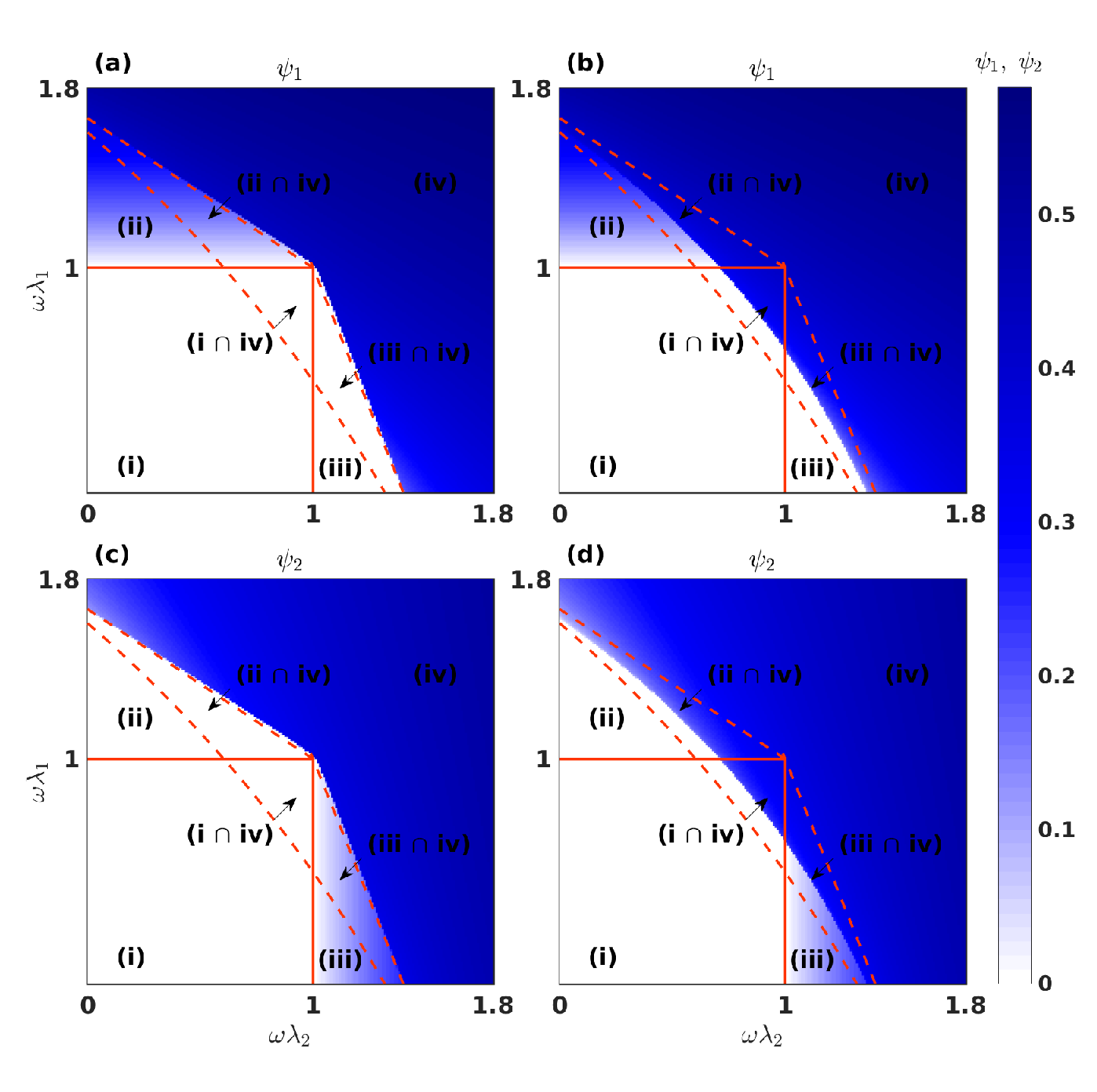
Are the phase diagrams obtained from the reduced mean field equations accurate in comparison with those from the original mean field equations? In the presence of the fluctuation terms $R_{a}$ , Eqs. (11) are exactly equivalent to Eqs. (1). Consider a system of dimension $2N+2$ , which consists of Eqs. (1) and Eqs. (11). A stable equilibrium point $\left(p_{1,i},p_{2,i}\right)_{1\leq i\leq N}$ of the subsystem Eqs. (1) is also one for the $2N+2$ system with $\psi_{a}=\alpha^{T}p_{a}$ . Consider a stable equilibrium point with which neither epidemic has an outbreak. Substituting $p_{a,1}=\cdots=p_{a,N}=0$ and $\psi_{a}=0$ into the remainder term (with full expression in Sec. II.2), we have $R_{a}=0$ for $a\in\{1,2\}$ . In this case the remainder terms can be ignored. Since a zero stable equilibrium point of Eqs. (1) implies the existence of exactly such a point of Eqs. (11) (with no remainder terms) and vice versa, any outbreak transition threshold from phase (i) is expected to be exact for Eqs. (1).

There are two cases where the remainder terms do not vanish and can lead to inaccuracies of the analytic prediction. The first case is when Eqs. (1) exhibit a stable equilibrium point at which there is an outbreak for epidemic $1$ but extinction for epidemic $2$ : $R_{1}=0$ and $R_{2}\neq 0$ . The second case is when Eqs. (1) have a stable equilibrium point with an outbreak for both epidemics: $R_{a}\neq 0$ for $a\in\{1,2\}$ . Since the remainder terms are small by construction, they lead to corrections that can be neglected, which have been verified numerically. Especially, for the Erdős-Rényi network in Fig. 1, we solve Eqs. (1) numerically and compare the solutions with the analytic phase diagram obtained from Eqs. (11). The values of $\psi_{a}$ obtained from Eqs. (1) in the $\lambda_{1}$ - $\lambda_{2}$ plane are shown in Figs. 2(a-d), for $\lambda_{1}^{\dagger}=3.5\omega^{-1}$ and $\lambda_{2}^{\dagger}=2.5\omega^{-1}$ [so that (102) is satisfied, guaranteeing a hysteresis]. Since in the hysteresis region there are two stable equilibrium points for each $\psi_{a}$ , we plot separately the two solutions for $\psi_{1}$ in Figs. 2(a) and 2(b), and those for $\psi_{2}$ in Figs. 2(c) and 2(d), respectively. The phase diagram from original Eqs. (11) is also shown in Fig. 2 by the orange solid and dashed lines for continuous and discontinuous transitions, respectively. Our analytical phase diagram predicts accurately all outbreak transitions: (i) $\ \to$ (ii), (i) $\ \to$ (iii), (i $\ \cap$ iv) $\ \to$ (iv), (ii $\ \cap$ iv) $\ \to$ (iv) and (iii $\ \cap$ iv) $\ \to$ (iv). However, quantitatively, the predicted extinction transitions (i $\ \cap$ iv) $\ \to$ (i), (ii $\ \cap$ iv) $\ \to$ (ii) and (iii $\ \cap$ iv) $\ \to$ (iii) are less accurate, due to the nonzero remainders $R_{1}$ and $R_{2}$ as a result of the loss of stability of an equilibrium point with an outbreak for both epidemics. The values of the remainders $R_{1}$ and $R_{2}$ at equilibrium are shown in Figs. 2(e-h). The value of $R_{1}$ for the two solutions of $\psi_{1}$ are shown in Figs. 2(e) and 2(f), respectively. Similarly, $R_{2}$ for the two solutions of $\psi_{2}$ are shown in Figs. 2(g) and 2(h), respectively. The predictions are qualitatively correct.

Next we consider tests and validation of our analytic prediction from Eqs. (11) for a variety of networks, including synthetic networks with strong and weak degree heterogeneity, and real-world networks. For synthetic networks, we have already shown the results for an ER network. Here we also consider networks generated from the uncorrelated configuration model (UCM) with a power-law degree distribution $p(k)\sim k^{-\beta}$ . Specifically, we consider three networks with different degree exponents: (1) PL-2.3 with $\beta=2.3$ , (2) PL-3 with $\beta=3$ and (3) PL-4 with $\beta=4$ . For empirical networks, we have (4) Dolphins Lusseau et al. 2003, a social network of bottle-nose dolphins; (5) HIV Auerbach et al. 1984, a network of sexual contacts between people involved in the early spread of the human immunodeficiency virus (HIV); (6) Highschool Coleman 1964, a friendship network between boys in a small high school, and (7) Jazz Gleiser and Danon 2003, a collaboration network between Jazz musicians. The networks are downloaded from Ref. Kunegis 2013.

Basic features and parameters of the networks considered are listed in Table 1. Note that Highschool is a directed and weighted network. Here we simply take it as undirected by assuming that there is an undirected edge between node $i$ and $j$ if there is at least a directed edge between the two nodes in either direction, with the edge weights ignored.

Table 1: Basic topological features of seven real networks:

N

and

M

are the number of nodes and edges, respectively,

C

is the clustering coefficient Watts and Strogatz 1998,

r

is the assortative coefficient Newman 2002,

\langle k\rangle

is the average degree,

H

is the degree heterogeneity which defined as

H={\langle k^{2}\rangle}/{{\langle k\rangle}^{2}}

, and

\langle d\rangle

is the average shortest distance.

	$N$	$M$	$C$	$r$	$k_{\mathrm{max}}$	$\langle k\rangle$	$H$	$\langle d\rangle$
ER	100	200	0.025	0.027	9	4	1.228	3.436
PL-2.3	100	234	0.040	-0.077	10	4.680	1.162	3.095
PL-3	100	216	0.042	-0.005	10	4.320	1.164	3.239
PL-4	100	185	0.033	0.022	10	3.700	1.108	3.709
Dolphins	62	159	0.259	-0.043	12	5.130	1.327	3.357
HIV	40	41	0.042	-0.279	8	2.050	1.512	4.474
Highschool	70	274	0.465	0.083	19	7.829	1.190	2.640
Jazz	198	2742	0.618	0.021	100	27.697	1.396	2.236

For all the networks, we set $\lambda_{1}^{\dagger}=3.5\omega^{-1}$ and $\lambda_{2}^{\dagger}=2.5\omega^{-1}$ to guarantee the emergence of a hysteresis region. To have an idea of the size of the correction terms $R_{a}$ , we show the values of $R_{a}$ at equilibrium. The results of (1) PL-2.3 (2) PL-3, (3) PL-4, (4) Dolphins, (5) HIV, (6) Highschool and (7) Jazz are shown in Figs. (3), (4), (5), (6), (7), (8) and (9), respectively. In each figure, subfigures (a) and (b) correspond to the values of $\psi_{1}$ , while (e) and (f) are the corresponding values of $R_{1}$ . Similarly, (c) and (d) correspond to the values of $\psi_{2}$ , while (g) and (h) are the corresponding values of $R_{2}$ . We see that, for all the networks tested, the analytic phase diagram predicts quantitatively and accurately the outbreak transitions, while the predicted extinction transitions are qualitatively correct. The values of correction terms $R_{a}$ are near zero for the outbreak transitions, while have relatively larger magnitudes near extinction transitions.

V Discussion

We have analytically predicted the phase diagram of interacting SIS spreading dynamics using the technique of spectral dimension reduction and provided numerical validation. The analytic phase diagram elucidates the interplay between discontinuous transitions and hystereses as well as the emergence of tricritical points. This method can also be applied to study other interacting epidemic models. For general epidemic models, a one-dimensional description of each epidemics is not sufficient Laurence et al. 2019. Determining the number of macroscopic observables required for general epidemic models needs further exploration.

Previous theoretical methods for interacting spreading dynamics such as QMF theory Wang et al. 2003 employ $2N$ equations, where $N$ is the network size. For large networks, it is computationally demanding to solve the equations to determine the stability of the fixed points, as this requires manipulating the $2N\times 2N$ Jacobian matrix. It is thus infeasible to use the QMF to map out the phase diagram for interacting spreading dynamics on complex networks, preventing us from gaining a full understanding of the interplay between network topology and the spreading dynamical process as a full phase diagram would reveal. The same difficulty arises with a naive application of the SDR method Laurence et al. 2019 in order to obtain the phase diagram for interacting spreading dynamics. In contrast, our approach gives a full picture of the phase diagram on large complex networks with an arbitrary topology through an effective two-dimensional system, revealing rich phenomena that have not been systemically investigated. While many previous studies employed the mean-field theory to study different types of spreading dynamics on complex networks Pastor-Satorras and Vespignani 2001; Boguñá et al. 2003; Castellano and Pastor-Satorras 2006, our work is not a simple application of the mean-field theory. In fact, we go way beyond by obtaining, for the first time to our knowledge, a global phase diagram laying out a clear picture of all possible dynamical states and the transitions among them through a comprehensive stability analysis - both at an unprecedented level of details.

Taken together, our work gives a full picture of the dependence of phase transition on network topology and spreading parameters for SIS dynamics, and thus lays a foundation for intervening or harnessing this type of interacting spreading processes. For instance, our phase diagram gives possible routes for controlling the type of phase transition through perturbations to the network structure or for controlling one spreading process through manipulating another interacting process. It should be cautioned that, while the SIS model provides phenomenological insights into relatively simply spreading processes and is thus a conceptually useful paradigmatic model, it may be too simplistic to describe spreading processes in the real world which can be significantly more complicated. To apply our analytic approach to irreversible epidemic processes beyond the SIS dynamics is possible but remains to be studied.

Acknowledgments

This work was partially supported by NNSF of China under Grants Nos. 61903266, 61433014 and 61673086), China Postdoctoral Science Foundation under Grant No. 2018M631073, China Postdoctoral Science Special Foundation under Grant No. 2019T120829), the Science Strength Promotion Program of the University of Electronic Science and Technology of China under Grant No. Y030190261010020, and Fundamental Research Funds for the Central Universities. YCL is supported by ONR under Grant No. N00014-16-1-2828.

Appendix A: Proof for $\mu\geq 1$

To prove $\mu\geq 1$ , we rewrite Eq. (10) as

\mu^{-1}=\frac{\alpha^{T}G\alpha}{\alpha^{T}K\alpha}.

(A.1)

Since $K$ is positive definite, it can be decomposed as $K=K^{1/2}K^{1/2}$ , where $K^{1/2}$ is a diagonal matrix whose entries are the square root of the degrees. Let $y=K^{1/2}\alpha$ . We have $\alpha=K^{-1/2}y$ . Substituting this back to $\mu^{-1}$ gives

\mu^{-1}=\frac{yK^{-1/2}GK^{-1/2}y}{y^{T}y},

(A.2)

which is the Rayleigh quotient of matrix $K^{-1/2}GK^{-1/2}$ and, hence, we have $\mu^{-1}\leq\delta_{1}$ , where $\delta_{1}$ is the largest eigenvalue of the matrix $K^{-1/2}GK^{-1/2}$ . Recall that the symmetric normalized Laplacian matrix of $G$ is defined as

L^{\mathrm{sym}}=I-K^{-1/2}GK^{-1/2},

(A.3)

which has a smallest eigenvalue $\zeta_{n}=0$ . As a result, we have $\delta_{1}=1-\zeta_{n}=1$ , which gives $\mu\geq 1$ .

References

Ferguson et al. (2003) N. M. Ferguson, A. P. Galvani, and R. M. Bush, “Ecological and immunological determinants of influenza evolution,” Nature 422, 428 (2003).
Abu-Raddad et al. (2006) L. J. Abu-Raddad, P. Patnaik, and J. G. Kublin, “Dual infection with HIV and malaria fuels the spread of both diseases in sub-Saharan Africa,” Science 314, 1603 (2006).
Funk et al. (2009) S. Funk, E. Gilad, C. Watkins, and V. A. Jansen, “The spread of awareness and its impact on epidemic outbreaks,” Proc. Nat. Acad. Sci. (USA) 106, 6872 (2009).
Gog and Grenfell (2002) J. R. Gog and B. T. Grenfell, “Dynamics and selection of many-strain pathogens,” Proc. Nat. Acad. Sci. (USA) 99, 17209 (2002).
Eames and Keeling (2006a) K. T. Eames and M. J. Keeling, “Coexistence and specialization of pathogen strains on contact networks,” Am. Nat. 168, 230 (2006a).
Berkman et al. (2014) L. F. Berkman, I. Kawachi, and M. M. Glymour, Social Epidemiology (Oxford University Press, 2014).
Sanz et al. (2014) J. Sanz, C.-Y. Xia, S. Meloni, and Y. Moreno, “Dynamics of interacting diseases,” Phys. Rev. X 4, 041005 (2014).
Pastor-Satorras et al. (2015) R. Pastor-Satorras, C. Castellano, P. Van Mieghem, and A. Vespignani, “Epidemic processes in complex networks,” Rev. Mod. Phys. 87, 925 (2015).
de Arruda et al. (2018) G. F. de Arruda, F. A. Rodrigues, and Y. Moreno, “Fundamentals of spreading processes in single and multilayer complex networks,” Phys. Rep. 756, 1 (2018).
Wang et al. (2019) W. Wang, Q.-H. Liu, J. Liang, Y. Hu, and T. Zhou, “Coevolution spreading in complex networks,” arXiv:1901.02125 (2019).
Soriano-Paños et al. (2019) D. Soriano-Paños, F. Ghanbarnejad, S. Meloni, and J. Gómez-Gardeñes, “Markovian approach to tackle the interaction of simultaneous diseases,” Phys. Rev. E 100, 062308 (2019).
Eames and Keeling (2006b) K. T. D. Eames and M. J. Keeling, “Coexistence and specialization of pathogen strains on contact networks,” Amer. Nat. 168, 230 (2006b).
Danziger et al. (2019) M. M. Danziger, I. Bonamassa, S. Boccaletti, and S. Havlin, “Dynamic interdependence and competition in multilayer networks,” Nat. Phys. 15, 178 (2019).
Soriano-Paños et al. (2019) D. Soriano-Paños, F. Ghanbarnejad, S. Meloni, and J. Gómez-Gardeñes, “Markovian approach to tackle the interaction of simultaneous diseases,” Phys. Rev. E 100, 062308 (2019).
Cai et al. (2015) W. Cai, L. Chen, F. Ghanbarnejad, and P. Grassberger, “Avalanche outbreaks emerging in cooperative contagions,” Nat. Phys. 11, 936 (2015).
Noh and Park (2005) J. D. Noh and H. Park, “Asymmetrically coupled directed percolation systems,” Phys. Rev. Lett. 94, 145702 (2005).
Granell et al. (2013) C. Granell, S. Gómez, and A. Arenas, “Dynamical interplay between awareness and epidemic spreading in multiplex networks,” Phys. Rev. Lett. 111, 128701 (2013).
Wang et al. (2014) W. Wang, M. Tang, H. Yang, Y. Do, Y.-C. Lai, and G. Lee, “Asymmetrically interacting spreading dynamics on complex layered networks,” Sci. Rep. 4, 5097 (2014).
Hébert-Dufresne and Althouse (2015) L. Hébert-Dufresne and B. M. Althouse, “Complex dynamics of synergistic coinfections on realistically clustered networks,” Proc. Nat. Acad. Sci. (USA) 112, 10551 (2015).
Chen (2019) L. Chen, “Persistent spatial patterns of interacting contagions,” Phys. Rev. E 99, 022308 (2019).
Castellano et al. (2009) C. Castellano, S. Fortunato, and V. Loreto, “Statistical physics of social dynamics,” Rev. Mod. Phys. 81, 591 (2009).
Dorogovtsev et al. (2008) S. N. Dorogovtsev, A. V. Goltsev, and J. F. F. Mendes, “Critical phenomena in complex networks,” Rev. Mod. Phys. 80, 1275 (2008).
Kiss et al. (2017) I. Z. Kiss, J. C. Miller, and P. L. Simon, Mathematics of Epidemics on Networks (Springer-Verlag, New York-Heidelberg-Dordrecht-London, 2017).
Abu-Raddad et al. (2008) L. Abu-Raddad, B. Van der Ventel, and N. Ferguson, “Interactions of multiple strain pathogen diseases in the presence of coinfection, cross immunity, and arbitrary strain diversity,” Phys. Rev. Lett. 100, 168102 (2008).
Zarei et al. (2019) F. Zarei, S. Moghimi-Araghi, and F. Ghanbarnejad, “Exact solution of generalized cooperative susceptible-infected-removed (SIR) dynamics,” Phys. Rev. E 100, 012307 (2019).
Prakash et al. (2012a) B. A. Prakash, A. Beutel, R. Rosenfeld, and C. Faloutsos, “Winner takes all: Competing viruses or ideas on fair-play networks,” in Proceedings of the 21st International Conference on World Wide Web, WWW’12 (ACM, 2012) pp. 1037–1046.
Newman (2005) M. E. Newman, “Threshold effects for two pathogens spreading on a network,” Phys. Rev. Lett. 95, 108701 (2005).
Chen et al. (2013) L. Chen, F. Ghanbarnejad, W. Cai, and P. Grassberger, “Outbreaks of coinfections: The critical role of cooperativity,” Europhys. Lett. 104, 50001 (2013).
Sahneh and Scoglio (2014) F. D. Sahneh and C. Scoglio, “Competitive epidemic spreading over arbitrary multilayer networks,” Phys. Rev. E 89, 062817 (2014).
Granell et al. (2014) C. Granell, S. Gómez, and A. Arenas, “Competing spreading processes on multiplex networks: awareness and epidemics,” Phys. Rev. E 90, 012808 (2014).
Van Mieghem (2011) P. Van Mieghem, “The n-intertwined SIS epidemic network model,” Computing 93, 147 (2011).
Achlioptas et al. (2009) D. Achlioptas, R. M. D’Souza, and J. Spencer, “Explosive percolation in random networks,” Science 323, 1453 (2009).
da Costa et al. (2010) R. A. da Costa, S. N. Dorogovtsev, A. V. Goltsev, and J. F. F. Mendes, “Explosive percolation transition is actually continuous,” Phys. Rev. Lett. 105, 255701 (2010).
Gao et al. (2016) J. Gao, B. Barzel, and A.-L. Barabási, “Universal resilience patterns in complex networks,” Nature 530, 307 (2016).
Laurence et al. (2019) E. Laurence, N. Doyon, L. J. Dubé, and P. Desrosiers, “Spectral dimension reduction of complex dynamical networks,” Phys. Rev. X 9, 011042 (2019).
Jiang et al. (2018) J. Jiang, Z.-G. Huang, T. P. Seager, W. Lin, C. Grebogi, A. Hastings, and Y.-C. Lai, “Predicting tipping points in mutualistic networks through dimension reduction,” Proc. Nat. Acad. Sci. (USA) 115, E639 (2018).
Chen et al. (2017) L. Chen, F. Ghanbarnejad, and D. Brockmann, “Phase transitions and hysteresis of cooperative contagion processes,” New J. Phys. 19, 103041 (2017).
Wang et al. (2003) Y. Wang, D. Chakrabarti, C. Wang, and C. Faloutsos, “Epidemic spreading in real networks: An eigenvalue viewpoint,” in Proceedings of the 22nd International Symposium on Reliable Distributed Systems (IEEE, 2003) pp. 25–34.
Boguná et al. (2013) M. Boguná, C. Castellano, and R. Pastor-Satorras, “Nature of the epidemic threshold for the susceptible-infected-susceptible dynamics in networks,” Phys. Rev. Lett. 111, 068701 (2013).
Prakash et al. (2012b) B. A. Prakash, A. Beutel, R. Rosenfeld, and C. Faloutsos, “Winner takes all: competing viruses or ideas on fair-play networks,” in Proceedings of the 21st international conference on World Wide Web (2012) pp. 1037–1046.
Lusseau et al. (2003) D. Lusseau, K. Schneider, O. J. Boisseau, P. Haase, E. Slooten, and S. M. Dawson, “The bottlenose dolphin community of doubtful sound features a large proportion of long-lasting associations,” Behav. Ecol. and Sociobiol 54, 396 (2003).
Auerbach et al. (1984) D. M. Auerbach, W. W. Darrow, H. W. Jaffe, and J. W. Curran, “Cluster of cases of the acquired immune deficiency syndrome: Patients linked by sexual contact,” Am. J. Med. 76, 487 (1984).
Coleman (1964) J. S. Coleman, Introduction to Mathematical Sociology (London Free Press Glencoe, 1964).
Gleiser and Danon (2003) P. M. Gleiser and L. Danon, “Community structure in jazz,” Adv. Comp. Sys. 6, 565 (2003).
Kunegis (2013) J. Kunegis, “Konect: the koblenz network collection,” in Proceedings of the 22nd International Conference on World Wide Web (2013) pp. 1343–1350.
Watts and Strogatz (1998) D. J. Watts and S. H. Strogatz, “Collective dynamics of ’small-world’ networks,” Nature 393, 440 (1998).
Newman (2002) M. E. J. Newman, “Assortative mixing in networks,” Phys. Rev. Lett. 89, 208701 (2002).
Pastor-Satorras and Vespignani (2001) R. Pastor-Satorras and A. Vespignani, “Epidemic spreading in scale-free networks,” Phys. Rev. Lett. 86, 3200 (2001).
Boguñá et al. (2003) M. Boguñá, R. Pastor-Satorras, and A. Vespignani, “Absence of epidemic threshold in scale-free networks with degree correlations,” Phys. Rev. Lett. 90, 028701 (2003).
Castellano and Pastor-Satorras (2006) C. Castellano and R. Pastor-Satorras, “Non-mean-field behavior of the contact process on scale-free networks,” Phys. Rev. Lett. 96, 038701 (2006).

Phase diagrams of interacting spreading dynamics in complex networks

Abstract

I Introduction

II Model, method of spectral dimension reduction, and reduced model

II.1 Model

II.2 Spectral dimension reduction

II.3 Reduced model

III Main result: phase diagram of reduced system

III.1 Equilibrium points of the reduced system

III.2 Stability analysis

III.3 Phase diagrams

III.4 Types of phase transition

III.5 Conditions on λa†\lambda_{a}^{\dagger} for hysteresis

III.6 Summary of the phase diagrams

(i) Epidemic free region.

(ii) Partial infection of epidemic 11.

(iii) Partial infection of epidemic 22.

(iv) Coexistence.

(i∩\ \cap iv) Hysteresis region 1.

(ii∩\ \cap iv) Hysteresis region 2.

(iii∩\ \cap iv) Hysteresis region 3.

IV Numerical verification

V Discussion

Acknowledgments

Appendix A: Proof for μ≥1\mu\geq 1

References

III.5 Conditions on $\lambda_{a}^{\dagger}$ for hysteresis

(ii) Partial infection of epidemic $1$ .

(iii) Partial infection of epidemic $2$ .

(i $\ \cap$ iv) Hysteresis region 1.

(ii $\ \cap$ iv) Hysteresis region 2.

(iii $\ \cap$ iv) Hysteresis region 3.

Appendix A: Proof for $\mu\geq 1$