跳到论文正文
W Papers独立论文阅读器 arXiv:2001.09443 论文正文 计算阅读时间 · 0%
引用这篇论文根据当前论文元数据生成,正式投稿前建议核对。


License: arXiv.org perpetual non-exclusive license
arXiv:2001.09443v2 [q-fin.PR] 18 Jun 2020

Pricing vulnerable options in a hybrid credit risk model driven by Heston-Nandi GARCH processes Gechun Liang is at Department of Statistics, University of Warwick, Coventry CV4 7AL, UK. Xingchun Wang is at the School of International Trade and Economics, University of International Business and Economics, Beijing 100029, China. This study was supported by the National Natural Science Foundation of China (Nos. 11701084 and 11671084) and Excellent Young Scholars Program in University of International Business and Economics (17YQ01).

GECHUN LIANG    XINGCHUN WANG Note: Correspondence address, Office 416, Qiuzhen Building, University of International Business and Economics, Beijing 100029, China. Email: xchwangnk@aliyun.com; wangx@uibe.edu.cn
Abstract

This paper proposes a hybrid credit risk model, in closed form, to price vulnerable options with stochastic volatility. The distinctive features of the model are threefold. First, both the underlying and the option issuer’s assets follow the Heston-Nandi GARCH model with their conditional variance being readily estimated and implemented solely on the basis of the observable prices in the market. Second, the model incorporates both idiosyncratic and systematic risks into the asset dynamics of the underlying and the option issuer, as well as the intensity process. Finally, the explicit pricing formula of vulnerable options enables us to undertake the comparative statistics analysis.

Keywords: Vulnerable options; hybrid credit risk model; Heston-Nandi GARCH model; closed form formula.

JEL classification : G13

1 Introduction

Vulnerable options refer to financial derivatives subject to default risk of the option’s issuers, and they are widely traded in over-the-counter (OTC) markets. As of the first half of 2019, 3.9 trillion dollars (in terms of notional amounts) option contacts were traded in OTC markets11 1 Resource: BIS, OTC derivatives statistics, https://www.bis.org/statistics/derstats.htm. The bespoke nature and the flexibility in terms of product design have helped OTC markets to thrive. As opposed to exchange-traded derivatives for which products are limited in tenor, size and strike ranges, OTC derivatives facilitate tailoring of transactions to meet specific end-users’ needs. In this paper, we study vulnerable options with stochastic volatility in a hybrid credit risk model driven by GARCH processes.

In order to study default risk of options, two types of models are widely used: structural models and reduced-form models. Johnson and Stulz (1987) first investigate vulnerable options using the structural approach, where default happens when the value of the option at maturity exceeds the value of the option issuer’s assets, resulting in the failure of the option issuer to honor their obligation. This assumption is relaxed by Klein (1996), where the option issuer could hold other liabilities having the same priority as the option. Vast majority of research focuses on the structural framework by taking into account of more factors such as stochastic interest rate, jump risk, stochastic volatility, stochastic default barriers, and multiple counterparties22 2 A partial list of the studies on this topic includes Rich (1996), Klein and Inglis (1999), Klein and Inglis (2001), Cao and Wei (2001), Hui et al. (2003), Liao and Huang (2005), Kao (2006), Liang and Ren (2007), Xu et al. (2012), Tian et al. (2014), Yang et al. (2014), Lee et al. (2016), Wang (2016), Wang et al. (2017), and Wang (2018).. One attractive feature of the structural approach is its ability to explain default events via the structural variables such as asset dynamics.

As opposed to the structural approach, the reduced-form models are silent about why defaults happen and, instead, the dynamics of default are exogenously given through a default rate, i.e. the default intensity. The latter approach is also called intensity approach. In contrast to the reduced-form approach for bond pricing where the payoff is a fixed income, the payoff of vulnerable options is random, so it is more challenging in reduced-form models to obtain an explicit pricing formula of vulnerable options. There are relatively few results in this direction. To name a few, Hull and White (1995) impose an independence assumption to obtain a closed-form pricing formula of vulnerable options; Fard (2015) obtains a closed-form price for vulnerable options by assuming that the default intensity is captured by a mean-reverting Ornstein-Uhlenbeck process (so a negative intensity is allowed); Antonelli et al. (2020) employ a correlation expansion approach to provide an approximate evaluation of vulnerable option prices; and Wang (2017) obtains a closed-form solution for vulnerable options in a discrete-time GARCH framework.

In this paper, we consider vulnerable options in a hybrid credit risk model. The model will incorporate the attractive features of both structural and reduced-form models. Hybrid credit risk models were initiated by Madan and Unal (2000), who investigate the pricing issue of risky debt in a hazard rate model with two factors being the values of the firm’s assets and the interest rate. Bakshi et al. (2006) further work under a reduced-form model based on Vasicek-type state variables, such as leverage, book-to-market and equity-volatility. Gu et al. (2014) consider a new type of reduced-form model that incorporates the impacts of observable trigger events as well as economic environment on corporate defaults. Boudreault et al. (2014) measure how contagion affects default time and recovery rates in a hybrid model, where both the default probability and the recovery rate are functions of the firm’s leverage ratio. However, the above mentioned studies mainly focus on risky debt or credit derivatives. The aim of the current paper is to propose a hybrid credit risk model for vulnerable options with the aforementioned reduced-form model as a special case of the proposed hybrid credit risk model.

In our model, the dynamics of the underlying and the option issuer’s assets follow the Heston-Nandi GARCH processes to incorporate stochastic volatility. As pointed out in Heston and Nandi (2000) and Hsieh and Ritchken (2005), the continuous time stochastic volatility models are difficult to implement and test, while GARCH models have inherent advantages that the volatility is readily observable from the history of asset prices. We assume that the asset values of both underlying and option issuer are exposed to idiosyncratic and systematic risks. Furthermore, we also allow the intensity process to be driven by idiosyncratic shocks of the issuer and systematic shocks of the market. Thus, the systematic risk factor correlates all the underlying processes in the proposed hybrid model.

Under this framework, we obtain an explicit pricing formula of vulnerable options based on the explicit expression of the joint generating function and the change of measure technique. The joint generating function (see Proposition 2.1) generalizes the generating function for a single stock case in Heston and Nandi (2000) to a multidimensional case including the underlying stock, the issuer’s assets and the intensity process. Finally, we undertake comparative statistics analysis to investigate the effects of default risk on the option prices, and compare them with the default-free option prices and the ones obtained in the reduced-form model. One of the striking features is that the option prices increase with the sensitivity of the issuer’s assets to systematic risk, albeit a higher value of the sensitivity means that the issuer’s assets are more risky, resulting in a higher possibility of default. This is because a larger value of sensitivity also means the underlying asset and the issuer’s assets are more likely to be correlated, which in turn makes option issuers less likely to default when call options end in the money, yielding a higher option price consequently.

The remainder of this paper is organized as follows. In the coming section, we focus on the hybrid credit risk model and the derivation of the explicit pricing formulae. Section 3 is devoted to numerical results. Finally, Section 4 summarizes and concludes the paper. The detailed proofs are shown in the appendix.

2 The hybrid credit risk model

In this section, we propose a hybrid credit risk model to price vulnerable options. An explicit pricing formula of vulnerable options is derived based on the change of measure technique and the explicit expression of the joint characteristic function of underlying processes.

2.1 The market

Let QQ be a risk neutral probability measure on a filtered probability space (Ω,ℱ,(ℱt)t≥0,Q)(\Omega,{\mathcal{F}},({\mathcal{F}}_{t})_{t\geq 0},Q). Consider a market with the systematic risk factor modelled by the market index M⁡(t)M(t), whose dynamics follow the Heston-Nandi GARCH process, that is,

{ln⁡M⁡(t)=ln⁡M⁡(t−1)+r−12​hm​(t)+hm​(t)​Zm​(t),hm​(t)=wm+bm​hm​(t−1)+am​(Zm​(t−1)−cm​hm​(t−1))2,\displaystyle\left\{\begin{array}[]{ll}\ln M(t)=\ln M(t-1)+r-\frac{1}{2}h_{m}(t)+\sqrt{h_{m}(t)}Z_{m}(t),\\ h_{m}(t)=w_{m}+b_{m}h_{m}(t-1)+a_{m}\Big(Z_{m}(t-1)-c_{m}\sqrt{h_{m}(t-1)}\Big)^{2},\end{array}\right.

where rr is the continuously compounded interest rate for the time interval [t−1,t][t-1,t], and Zm​(t)Z_{m}(t) is a standard normal random variable. The conditional variance hm​(t)h_{m}(t) of the log return between t−1t-1 and tt is known from the information set at time t−1t-1, so it can be readily estimated and implemented solely on the basis of the observables. In the driving noise term of hm​(t)h_{m}(t), the constant ama_{m} determines the kurtosis of the noise, and the constant cmc_{m} results in asymmetric influence of the noise Zm​(t−1)Z_{m}(t-1).

It has been shown in Heston and Nandi (2000) that the continuous time limit of the conditional variance hm​(t)h_{m}(t) is a square-root diffusion process corresponding to the continuous time Heston stochastic volatility model. On the other hand, it is clear that the discounted price of the market index is a martingale under QQ. Indeed, we have

Et−1​[M​(t)]\displaystyle E_{t-1}\Big[M(t)\Big] =\displaystyle= Et−1​[M⁡(t−1)​er−12​hm​(t)+hm​(t)​Zm​(t)]\displaystyle E_{t-1}\Big[M(t-1)e^{r-\frac{1}{2}h_{m}(t)+\sqrt{h_{m}(t)}Z_{m}(t)}\Big]
=\displaystyle= M⁡(t−1)​er​Et−1​[e−12​hm​(t)+hm​(t)​Zm​(t)]\displaystyle M(t-1)e^{r}E_{t-1}\Big[e^{-\frac{1}{2}h_{m}(t)+\sqrt{h_{m}(t)}Z_{m}(t)}\Big]
=\displaystyle= M⁡(t−1)​er,\displaystyle M(t-1)e^{r},

where in the last equality we have used the fact that hm​(t)h_{m}(t) is known given the information at time t−1t-1 and Zm​(t)Z_{m}(t) is a standard normal variable.

Consider a stock in this market. Its return is affected by not only the systematic risk factor via Zm​(t)Z_{m}(t) but also the idiosyncratic risk factor via an independent normal random variable Zs​(t)Z_{s}(t). Hence, the stock price S⁡(t)S(t) under QQ is driven by the process

{ln⁡S⁡(t)=ln⁡S⁡(t−1)+r−12​hs​(t)+hs​(t)​Zs​(t)−12​βs2​hm​(t)+βs​hm​(t)​Zm​(t),hs​(t)=ws+bs​hs​(t−1)+as​(Zs​(t−1)−cs​hs​(t−1))2,\displaystyle\left\{\begin{array}[]{ll}\ln S(t)=\ln S(t-1)+r-\frac{1}{2}h_{s}(t)+\sqrt{h_{s}(t)}Z_{s}(t)-\frac{1}{2}\beta_{s}^{2}h_{m}(t)+\beta_{s}\sqrt{h_{m}(t)}Z_{m}(t),\\ h_{s}(t)=w_{s}+b_{s}h_{s}(t-1)+a_{s}\Big(Z_{s}(t-1)-c_{s}\sqrt{h_{s}(t-1)}\Big)^{2},\end{array}\right.

where the constant βs\beta_{s} captures the sensitivity of the stock price to systematic risk. Since hm​(t)h_{m}(t) and hs​(t)h_{s}(t) are known given the information at time t−1t-1, the independence assumption between Zm​(t)Z_{m}(t) and Zs​(t)Z_{s}(t) implies that the discounted value of S⁡(t)S(t) is also a martingale under QQ,

Et−1​[S⁡(t)S⁡(t−1)]\displaystyle E_{t-1}\Big[\frac{S(t)}{S(t-1)}\Big] =\displaystyle= Et−1​[er−12​hs​(t)+hs​(t)​Zs​(t)−12​βs2​hm​(t)+βs​hm​(t)​Zm​(t)]\displaystyle E_{t-1}\Big[e^{r-\frac{1}{2}h_{s}(t)+\sqrt{h_{s}(t)}Z_{s}(t)-\frac{1}{2}\beta_{s}^{2}h_{m}(t)+\beta_{s}\sqrt{h_{m}(t)}Z_{m}(t)}\Big]
=\displaystyle= er​Et−1​[e−12​hs​(t)+hs​(t)​Zs​(t)]​Et−1​[e−12​βs2​hm​(t)+βs​hm​(t)​Zm​(t)]\displaystyle e^{r}E_{t-1}\Big[e^{-\frac{1}{2}h_{s}(t)+\sqrt{h_{s}(t)}Z_{s}(t)}\Big]E_{t-1}\Big[e^{-\frac{1}{2}\beta_{s}^{2}h_{m}(t)+\beta_{s}\sqrt{h_{m}(t)}Z_{m}(t)}\Big]
=\displaystyle= er.\displaystyle e^{r}.

We consider a European call option written on the stock with strike price KK and maturity TT, so its risk neutral price is given by E⁡[e−r​T​(S⁡(T)−K)+]E[e^{-rT}(S(T)-K)^{+}] if the option issuer does not default during the contract period and is able to honor their obligation. Note that under the above GARCH framework, Heston and Nandi (2000) derived an explicit pricing formula for the European call option using the characteristic function of S⁡(t)S(t) (see section 2 therein).

2.2 The vulnerable option with credit value adjustment

When the options are traded in OTC markets, the holders may face the potential default risk that the issuers are not able to deliver the promised payoff. We model the default risk in a hybrid model. To this end, let N⁡(t)N(t) be a doubly stochastic Poisson process (Cox process) with intensity Λ⁡(t)\Lambda(t), and τ\tau be its first jump time which can be regarded as the arrival time of the default trigger event as in Gu et al. (2014). A loss given default (LGD) will occur when the trigger event arrives, and it is given by a constant LL. Furthermore, assume that the option issuer would recover from the trigger event if the value of the issuer’s assets is larger than the LGD LL. Hence, default occurs only when the trigger event occurs and the value of the issuer’s assets at the arrival time of the trigger event falls below the LGD LL.

Next, we model the option issuer’s assets V⁡(t)V(t) and the Cox process’ intensity Λ⁡(t)\Lambda(t). Assume that the return of the issuer’s assets is also affected by both the systematic and idiosyncratic risks and its dynamics follow

{ln⁡V⁡(t)=ln⁡V⁡(t−1)+r−12​hv​(t)+hv​(t)​Zv​(t)−12​βv2​hm​(t)+βv​hm​(t)​Zm​(t),hv​(t)=wv+bv​hv​(t−1)+av​(Zv​(t−1)−cv​hv​(t−1))2,\displaystyle\left\{\begin{array}[]{ll}\ln V(t)=\ln V(t-1)+r-\frac{1}{2}h_{v}(t)+\sqrt{h_{v}(t)}Z_{v}(t)-\frac{1}{2}\beta_{v}^{2}h_{m}(t)+\beta_{v}\sqrt{h_{m}(t)}Z_{m}(t),\\ h_{v}(t)=w_{v}+b_{v}h_{v}(t-1)+a_{v}\Big(Z_{v}(t-1)-c_{v}\sqrt{h_{v}(t-1)}\Big)^{2},\end{array}\right.

where Zv​(t)Z_{v}(t) is a standard normal variable independent of Zs​(t)Z_{s}(t) and Zm​(t)Z_{m}(t). Note that Zm​(t)Z_{m}(t) captures the systematic risk, and Zs​(t)Z_{s}(t) and Zv​(t)Z_{v}(t) represent the idiosyncratic risks of the underlying asset and the issuer’s assets, respectively. Similarly to βs\beta_{s} in (2.1), βv\beta_{v} captures the sensitivity of the issuer’s assets to the systematic risk. As for the intensity process Λ⁡(t)\Lambda(t), we assume that it is driven by Zv​(t)Z_{v}(t) and Zm​(t)Z_{m}(t), the driving noise faced by the issuer. Specifically, the dynamics of Λ⁡(t)\Lambda(t) are given by

Λ⁡(t+1)=wλ+bλ​Λ​(t)+aλ​(Zm​(t))2+cλ​(Zv​(t))2.\displaystyle\Lambda(t+1)=w_{\lambda}+b_{\lambda}\Lambda(t)+a_{\lambda}(Z_{m}(t))^{2}+c_{\lambda}(Z_{v}(t))^{2}. (2.8)

All the parameters are non-negative to ensure that the intensity is non-negative.

We are now in a position to present the hybrid credit risk model for the valuation of vulnerable options. To take account of the issuer’s default risk, we model the difference between the default-free value and the true value of the European option as follows: When j−1<τ≤j,V⁡(j)<Lj-1<\tau\leq j,\ V(j)<L, i.e. the trigger event occurs between (j−1,j](j-1,j] and the issuer’s asset value falls below the LGD, suppose the option holder will then only receive α​V​(j)/L\alpha V(j)/L proportion of the nominal payoff (S⁡(T)−K)+(S(T)-K)^{+} at the maturity TT, where the constant α∈[0,1]\alpha\in[0,1] represents the recovery rate and (1−α)​V​(j)(1-\alpha)V(j) represents the deadweight costs associated with the bankruptcy. Hence, the expected value of the credit value adjustment (i.e. the difference between the default-free value and the true value) is

E⁡[e−r​T​(1−α​V​(j)L)​(S⁡(T)−K)+].E\left[e^{-rT}(1-\frac{\alpha V(j)}{L})(S(T)-K)^{+}\right].

conditional on the event {j−1<τ≤j,V(i)<L}\{j-1<\tau\leq j,V(i)<L\}.

The price of the vulnerable option at time 00 is therefore given by

C0\displaystyle C_{0} =\displaystyle= E[e−r​T(S(T)−K)+]−∑j=1TE[e−r​TI(j−1<τ≤j,V(j)<L)(1−α​V​(j)L)(S(T)−K)+]\displaystyle E\Big[e^{-rT}(S(T)-K)^{+}\Big]-\sum_{j=1}^{T}E\Big[e^{-rT}I(j-1<\tau\leq j,\ V(j)<L)(1-\frac{\alpha V(j)}{L})(S(T)-K)^{+}\Big] (2.9)
=\displaystyle= E[e−r​T(S(T)−K)+]−∑j=1TE[e−r​TI(j−1<τ≤j,V(j)<L)(S(T)−K)+]\displaystyle E\Big[e^{-rT}(S(T)-K)^{+}\Big]-\sum_{j=1}^{T}E\Big[e^{-rT}I(j-1<\tau\leq j,\ V(j)<L)(S(T)-K)^{+}\Big]
+∑j=1TE[e−r​TI(j−1<τ≤j,V(j)<L)α​V​(j)L(S(T)−K)+],\displaystyle+\ \ \sum_{j=1}^{T}E\Big[e^{-rT}I(j-1<\tau\leq j,\ V(j)<L)\frac{\alpha V(j)}{L}(S(T)-K)^{+}\Big],

where I⁡(⋅)I(\cdot) is the indicator function. The first term in (2.9) is the default-free value, the second term represents the costs when default occurs, and the last term is the recovery value from the default. Note that I⁡(j−1<τ≤j)=I⁡(j−1<τ)−I⁡(j<τ)I(j-1<\tau\leq j)=I(j-1<\tau)-I(j<\tau), so the last two terms in (2.9) simplify to

E[I(j−1<τ≤j,V(j)<L)(S(T)−K)+]\displaystyle E\Big[I(j-1<\tau\leq j,\ V(j)<L)(S(T)-K)^{+}\Big]
=\displaystyle= E⁡[I⁡(j−1<τ≤j)​I​(V⁡(j)<L)​(S⁡(T)−K)+]\displaystyle E\Big[I(j-1<\tau\leq j)I(V(j)<L)(S(T)-K)^{+}\Big]
=\displaystyle= −E⁡[I⁡(j<τ)​I​(V⁡(j)<L)​(S⁡(T)−K)+]+E⁡[I⁡(j−1<τ)​I​(V⁡(j)<L)​(S⁡(T)−K)+]\displaystyle-E\Big[I(j<\tau)I(V(j)<L)(S(T)-K)^{+}\Big]+E\Big[I(j-1<\tau)I(V(j)<L)(S(T)-K)^{+}\Big]
=\displaystyle= −E[e−∑k=1jΛ(k)I(V(j)<L)(S(T)−K)+]+E[e−∑k=1j−1Λ(k)I(V(j)<L)(S(T)−K)+],\displaystyle-E\Big[e^{-\sum_{k=1}^{j}\Lambda(k)}I(V(j)<L)(S(T)-K)^{+}\Big]+E\Big[e^{-\sum_{k=1}^{j-1}\Lambda(k)}I(V(j)<L)(S(T)-K)^{+}\Big],

and

E[I(j−1<τ≤j,V(j)<L)α​V​(j)L(S(T)−K)+]\displaystyle E\Big[I(j-1<\tau\leq j,\ V(j)<L)\frac{\alpha V(j)}{L}(S(T)-K)^{+}\Big]
=\displaystyle= E⁡[I⁡(j−1<τ≤j)​I​(V⁡(j)<L)​α​V​(j)L​(S⁡(T)−K)+]\displaystyle E\Big[I(j-1<\tau\leq j)I(V(j)<L)\frac{\alpha V(j)}{L}(S(T)-K)^{+}\Big]
=\displaystyle= −E⁡[I⁡(j<τ)​I​(V⁡(j)<L)​α​V​(j)L​(S⁡(T)−K)+]\displaystyle-E\Big[I(j<\tau)I(V(j)<L)\frac{\alpha V(j)}{L}(S(T)-K)^{+}\Big]
+E⁡[I⁡(j−1<τ)​I​(V⁡(j)<L)​α​V​(j)L​(S⁡(T)−K)+]\displaystyle+E\Big[I(j-1<\tau)I(V(j)<L)\frac{\alpha V(j)}{L}(S(T)-K)^{+}\Big]
=\displaystyle= −E[e−∑k=1jΛ(k)I(V(j)<L)α​V​(j)L(S(T)−K)+]\displaystyle-E\Big[e^{-\sum_{k=1}^{j}\Lambda(k)}I(V(j)<L)\frac{\alpha V(j)}{L}(S(T)-K)^{+}\Big]
+E[e−∑k=1j−1Λ(k)I(V(j)<L)α​V​(j)L(S(T)−K)+].\displaystyle+E\Big[e^{-\sum_{k=1}^{j-1}\Lambda(k)}I(V(j)<L)\frac{\alpha V(j)}{L}(S(T)-K)^{+}\Big].

In turn, we have

C0\displaystyle C_{0} =\displaystyle= e−r​T​(E⁡[(S⁡(T)−K)+]CLOSE\displaystyle e^{-rT}\Big(E\Big[(S(T)-K)^{+}\Big] (2.10)
+∑j=1TE[e−∑k=1jΛ(k)I(V(j)<L)(S(T)−K)+]\displaystyle+\sum_{j=1}^{T}E\Big[e^{-\sum_{k=1}^{j}\Lambda(k)}I(V(j)<L)(S(T)-K)^{+}\Big]
−∑j=1TE[e−∑k=1j−1Λ(k)I(V(j)<L)(S(T)−K)+]\displaystyle-\sum_{j=1}^{T}E\Big[e^{-\sum_{k=1}^{j-1}\Lambda(k)}I(V(j)<L)(S(T)-K)^{+}\Big]
−∑j=1TE[e−∑k=1jΛ(k)I(V(j)<L)α​V​(j)L(S(T)−K)+]\displaystyle-\sum_{j=1}^{T}E\Big[e^{-\sum_{k=1}^{j}\Lambda(k)}I(V(j)<L)\frac{\alpha V(j)}{L}(S(T)-K)^{+}\Big]
+∑j=1TE[e−∑k=1j−1Λ(k)I(V(j)<L)α​V​(j)L(S(T)−K)+]).\displaystyle+\sum_{j=1}^{T}E\Big[e^{-\sum_{k=1}^{j-1}\Lambda(k)}I(V(j)<L)\frac{\alpha V(j)}{L}(S(T)-K)^{+}\Big]\Big).
Remark 2.1

In the proposed framework, the correlation coefficient between the underlying asset and the issuer’s assets is given by

Covt​(ln⁡S⁡(t+1)S⁡(t),ln⁡V⁡(t+1)V⁡(t))OPENVart​(ln⁡S⁡(t+1)S⁡(t))​Vart​(ln⁡V⁡(t+1)V⁡(t)CLOSE)\displaystyle\frac{{\rm Cov}_{t}(\ln\frac{S(t+1)}{S(t)},\ln\frac{V(t+1)}{V(t)})}{\sqrt{{\rm Var}_{t}(\ln\frac{S(t+1)}{S(t)})}\sqrt{{\rm Var}_{t}(\ln\frac{V(t+1)}{V(t)}})} =\displaystyle= Covt​(βs​hm​(t+1)​Zm​(t+1),βv​hm​(t+1)​Zm​(t+1))hs​(t+1)+βs2​hm​(t+1)​hv​(t+1)+βv2​hm​(t+1)\displaystyle\frac{{\rm Cov}_{t}(\beta_{s}\sqrt{h_{m}(t+1)}Z_{m}(t+1),\beta_{v}\sqrt{h_{m}(t+1)}Z_{m}(t+1))}{\sqrt{h_{s}(t+1)+\beta_{s}^{2}h_{m}(t+1)}\sqrt{h_{v}(t+1)+\beta_{v}^{2}h_{m}(t+1)}}
=\displaystyle= βs​βv​hm​(t+1)hs​(t+1)+βs2​hm​(t+1)​hv​(t+1)+βv2​hm​(t+1).\displaystyle\frac{\beta_{s}\beta_{v}h_{m}(t+1)}{\sqrt{h_{s}(t+1)+\beta_{s}^{2}h_{m}(t+1)}\sqrt{h_{v}(t+1)+\beta_{v}^{2}h_{m}(t+1)}}.

When βs=0\beta_{s}=0 or βv=0\beta_{v}=0, the underlying asset and the issuer’s assets are not correlated with each other. On the other hand, when hs​(t+1)≡0h_{s}(t+1)\equiv 0 (i.e. ws=bs=as=0w_{s}=b_{s}=a_{s}=0) and hv​(t+1)≡0h_{v}(t+1)\equiv 0 (i.e. wv=bv=av=0w_{v}=b_{v}=a_{v}=0), both the underlying asset and the issuer’s assets are only driven by Zm​(t)Z_{m}(t), and the correlation coefficient becomes to be ±1\pm 1. In this sense, we can view Zm​(t)Z_{m}(t) as a common risk factor in the returns on the underlying asset and the issuer’s assets, and the issuer could hedge the option position by directly trading the underlying asset. Thus, Zm​(t)Z_{m}(t) could represent not only the systematic risk factor (though such an interpretation is the most typical example).

2.3 The explicit pricing formula

In order to obtain an explicit pricing formula for vulnerable options in the proposed framework, we first derive the joint conditional generating function of the underlying processes. To this end, let f⁡(t,ϕ1,ϕ2,ϕ3,ϕ4)f(t;\phi_{1},\phi_{2},\phi_{3},\phi_{4}) denote the conditional generating function given below,

f⁡(t,ϕ1,ϕ2,ϕ3,ϕ4)=Et​[exp⁡{ϕ1​ln⁡S⁡(T)+ϕ2​ln⁡V⁡(j)+ϕ3​Λ​(j)+ϕ4​∑k=1j−1Λ⁡(k)}],f(t;\phi_{1},\phi_{2},\phi_{3},\phi_{4})=E_{t}\Big[\exp\Big\{\phi_{1}\ln S(T)+\phi_{2}\ln V(j)+\phi_{3}\Lambda(j)+\phi_{4}\sum_{k=1}^{j-1}\Lambda(k)\Big\}\Big],

where j≤Tj\leq T and 0≤t≤T0\leq t\leq T. Specially, f⁡(t,ϕ1,0,0,0)f(t;\phi_{1},0,0,0) is the conditional generating function of the underlying asset and can be used to derive the default-free value of the European option as in Heston and Nandi (2000). In addition, f⁡(t,ϕ1,0,ϕ3,ϕ4)f(t;\phi_{1},0,\phi_{3},\phi_{4}) can be employed to obtain the closed-form pricing formula of vulnerable options in the reduced-form models, which is a special case of the proposed hybrid credit risk model (see section 2.4).

In the proposed framework, the explicit expression of f⁡(t,ϕ1,ϕ2,ϕ3,ϕ4)f(t;\phi_{1},\phi_{2},\phi_{3},\phi_{4}) is available and given in the following proposition.

Proposition 2.1

The conditional generating function has the following form33 3 For convenience, we use the more parsimonious notation f⁡(t)f(t) to indicate f⁡(t,ϕ1,ϕ2,ϕ3,ϕ4)f(t;\phi_{1},\phi_{2},\phi_{3},\phi_{4}), and similarly for Ai​(t)A_{i}(t) and Bi​(t)B_{i}(t).

f⁡(t)\displaystyle f(t) =\displaystyle= exp{ϕ2lnV(j)+ϕ3Λ(j)+ϕ4∑k=1j−1Λ(k)+ϕ1lnS(t)+A0(t)\displaystyle\exp\Big\{\phi_{2}\ln V(j)+\phi_{3}\Lambda(j)+\phi_{4}\sum_{k=1}^{j-1}\Lambda(k)+\phi_{1}\ln S(t)+A_{0}(t) (2.11)
+A1(t)hm(t+1)+A2(t)hs(t+1)},\displaystyle\ \ \ \ \ \ \ \ \ \ \ +A_{1}(t)h_{m}(t+1)+A_{2}(t)h_{s}(t+1)\Big\},

for j≤t≤Tj\leq t\leq T, where A0​(t)A_{0}(t), A1​(t)A_{1}(t) and A2​(t)A_{2}(t) (j≤t≤Tj\leq t\leq T) are defined recursively with terminal conditions A0​(T)=A1​(T)=A2​(T)=0A_{0}(T)=A_{1}(T)=A_{2}(T)=0 by the following expressions

A0​(t)=\displaystyle A_{0}(t)= ϕ1​r+A0​(t+1)+wm​A1​(t+1)+ws​A2​(t+1)−12​ln⁡(1−2​am​A1​(t+1))\displaystyle\phi_{1}r+A_{0}(t+1)+w_{m}A_{1}(t+1)+w_{s}A_{2}(t+1)-\frac{1}{2}\ln(1-2a_{m}A_{1}(t+1))
−12​ln⁡(1−2​as​A2​(t+1)),\displaystyle-\frac{1}{2}\ln(1-2a_{s}A_{2}(t+1)),
A1​(t)=\displaystyle A_{1}(t)= bm​A1​(t+1)−12​ϕ1​βs2+ϕ1​βs​cm−12​cm2+12​(ϕ1​βs−cm)21−2​am​A1​(t+1),\displaystyle b_{m}A_{1}(t+1)-\frac{1}{2}\phi_{1}\beta_{s}^{2}+\phi_{1}\beta_{s}c_{m}-\frac{1}{2}c_{m}^{2}+\frac{\frac{1}{2}(\phi_{1}\beta_{s}-c_{m})^{2}}{1-2a_{m}A_{1}(t+1)},
A2​(t)=\displaystyle A_{2}(t)= bs​A2​(t+1)−12​ϕ1+ϕ1​cs−12​cs2+12​(ϕ1−cs)21−2​as​A2​(t+1).\displaystyle b_{s}A_{2}(t+1)-\frac{1}{2}\phi_{1}+\phi_{1}c_{s}-\frac{1}{2}c_{s}^{2}+\frac{\frac{1}{2}(\phi_{1}-c_{s})^{2}}{1-2a_{s}A_{2}(t+1)}.

For t<jt<j,

f⁡(t)\displaystyle f(t) =\displaystyle= exp{ϕ2lnV(t)+ϕ4∑k=1tΛ(k)+ϕ1lnS(t)+B0(t)\displaystyle\exp\Big\{\phi_{2}\ln V(t)+\phi_{4}\sum_{k=1}^{t}\Lambda(k)+\phi_{1}\ln S(t)+B_{0}(t) (2.12)
+B1(t)hm(t+1)+B2(t)hs(t+1)+B3(t)hv(t+1)+B4(t+1)Λ(t+1)},\displaystyle\ \ \ \ \ \ +B_{1}(t)h_{m}(t+1)+B_{2}(t)h_{s}(t+1)+B_{3}(t)h_{v}(t+1)+B_{4}(t+1)\Lambda(t+1)\Big\},

where Bk​(t),k=0,1,2,3,4B_{k}(t),\ k=0,1,2,3,4 (t<jt<j) can be obtained recursively by the following expressions

B0​(t)\displaystyle B_{0}(t) =\displaystyle= B0​(t+1)+(ϕ2+ϕ1)​r+wm​B1​(t+1)+ws​B2​(t+1)+wv​B3​(t+1)+wλ​B4​(t+1)\displaystyle B_{0}(t+1)+(\phi_{2}+\phi_{1})r+w_{m}B_{1}(t+1)+w_{s}B_{2}(t+1)+w_{v}B_{3}(t+1)+w_{\lambda}B_{4}(t+1)
OPEN−12​ln⁡(1−2​(am​B1​(t+1)+aλ​B4​(t+1)))−12​ln⁡(1−2​as​B2​(t+1)))\displaystyle\ \ \ -\frac{1}{2}\ln(1-2(a_{m}B_{1}(t+1)+a_{\lambda}B_{4}(t+1)))-\frac{1}{2}\ln(1-2a_{s}B_{2}(t+1)))
−12​ln⁡(1−2​(av​B3​(t+1)+cλ​B4​(t+1))),\displaystyle\ \ \ -\frac{1}{2}\ln(1-2(a_{v}B_{3}(t+1)+c_{\lambda}B_{4}(t+1))),
B1​(t)\displaystyle B_{1}(t) =\displaystyle= bm​B1​(t+1)−12​ϕ2​βv2−12​ϕ1​βs2+am​cm2​B1​(t+1)\displaystyle b_{m}B_{1}(t+1)-\frac{1}{2}\phi_{2}\beta_{v}^{2}-\frac{1}{2}\phi_{1}\beta_{s}^{2}+a_{m}c_{m}^{2}B_{1}(t+1)
+2​(am​cm​B1​(t+1)−(ϕ2​βv+ϕ1​βs)/2)21−2​(am​B1​(t+1)+aλ​B4​(t+1)),\displaystyle\ \ \ +\frac{2(a_{m}c_{m}B_{1}(t+1)-(\phi_{2}\beta_{v}+\phi_{1}\beta_{s})/2)^{2}}{1-2(a_{m}B_{1}(t+1)+a_{\lambda}B_{4}(t+1))},
B2​(t)\displaystyle B_{2}(t) =\displaystyle= bs​B2​(t+1)−12​ϕ1+as​cs2​B2​(t+1)+2​(as​cs​B2​(t+1)−ϕ1/2)21−2​as​B2​(t+1),\displaystyle b_{s}B_{2}(t+1)-\frac{1}{2}\phi_{1}+a_{s}c_{s}^{2}B_{2}(t+1)+\frac{2(a_{s}c_{s}B_{2}(t+1)-\phi_{1}/2)^{2}}{1-2a_{s}B_{2}(t+1)},
B3​(t)\displaystyle B_{3}(t) =\displaystyle= bv​B3​(t+1)−12​ϕ2+av​cv2​B3​(t+1)+2​(av​cv​B3​(t+1)−ϕ2/2)21−2​(av​B3​(t+1)+cλ​B4​(t+1)),\displaystyle b_{v}B_{3}(t+1)-\frac{1}{2}\phi_{2}+a_{v}c_{v}^{2}B_{3}(t+1)+\frac{2(a_{v}c_{v}B_{3}(t+1)-\phi_{2}/2)^{2}}{1-2(a_{v}B_{3}(t+1)+c_{\lambda}B_{4}(t+1))},
B4​(t)\displaystyle B_{4}(t) =\displaystyle= bλ​B4​(t+1)+ϕ4.\displaystyle b_{\lambda}B_{4}(t+1)+\phi_{4}.

Moreover, terminal conditions Bk​(j−1),k=0,1,2,3,4B_{k}(j-1),\ k=0,1,2,3,4 are determined by A0​(j)A_{0}(j), A1​(j)A_{1}(j) and A2​(j)A_{2}(j) as follows:

B0​(j−1)\displaystyle B_{0}(j-1) =\displaystyle= A0​(j)+(ϕ2+ϕ1)​r+wm​A1​(j)+ws​A2​(j)−12​ln⁡(1−2​am​A1​(j))−12​ln⁡(1−2​as​A2​(j)),\displaystyle A_{0}(j)+(\phi_{2}+\phi_{1})r+w_{m}A_{1}(j)+w_{s}A_{2}(j)-\frac{1}{2}\ln(1-2a_{m}A_{1}(j))-\frac{1}{2}\ln(1-2a_{s}A_{2}(j)),
B1​(j−1)\displaystyle B_{1}(j-1) =\displaystyle= bm​A1​(j)−12​ϕ2​βv2−12​ϕ1​βs2+am​cm2​A1​(j)+2​(am​cm​A1​(j)−(ϕ2​βv+ϕ1​βs)/2)21−2​am​A1​(j),\displaystyle b_{m}A_{1}(j)-\frac{1}{2}\phi_{2}\beta_{v}^{2}-\frac{1}{2}\phi_{1}\beta_{s}^{2}+a_{m}c_{m}^{2}A_{1}(j)+\frac{2(a_{m}c_{m}A_{1}(j)-(\phi_{2}\beta_{v}+\phi_{1}\beta_{s})/2)^{2}}{1-2a_{m}A_{1}(j)},
B2​(j−1)\displaystyle B_{2}(j-1) =\displaystyle= bs​A2​(j)−12​ϕ1+as​cs2​A2​(j)+2​(as​cs​A2​(j)−ϕ1/2)21−2​as​A2​(j),\displaystyle b_{s}A_{2}(j)-\frac{1}{2}\phi_{1}+a_{s}c_{s}^{2}A_{2}(j)+\frac{2(a_{s}c_{s}A_{2}(j)-\phi_{1}/2)^{2}}{1-2a_{s}A_{2}(j)},
B3​(j−1)\displaystyle B_{3}(j-1) =\displaystyle= −12​ϕ2+12​ϕ22,\displaystyle-\frac{1}{2}\phi_{2}+\frac{1}{2}\phi_{2}^{2},
B4​(j−1)\displaystyle B_{4}(j-1) =\displaystyle= ϕ3.\displaystyle\phi_{3}.

Proof. See the appendix.

We are ready to obtain the closed form pricing formula of the vulnerable option price in (2.9).

Theorem 2.1

The price of the vulnerable European call option with strike price KK and maturity TT is given by

C0\displaystyle C_{0} =\displaystyle= e−r​T​(12​f​(0,1,0,0,0)+1π​∫0∞Re​[e−i​ϕ1​ln⁡K​f​(0,1+i​ϕ1,0,0,0)i​ϕ1]​d​ϕ1CLOSE\displaystyle e^{-rT}\Big(\frac{1}{2}f(0;1,0,0,0)+\frac{1}{\pi}\int_{0}^{\infty}\textrm{Re}\Big[\frac{e^{-i\phi_{1}\ln K}f(0;1+i\phi_{1},0,0,0)}{i\phi_{1}}\Big]{\mathrm{d}}\phi_{1}
−K2−Kπ​∫0∞Re​[e−i​ϕ1​ln⁡K​f​(0,i​ϕ1,0,0,0)i​ϕ1]​d​ϕ1\displaystyle\ \ \ \ \ \ \ \ \ \ \ \ \ -\frac{K}{2}-\frac{K}{\pi}\int_{0}^{\infty}\textrm{Re}\Big[\frac{e^{-i\phi_{1}\ln K}f(0;i\phi_{1},0,0,0)}{i\phi_{1}}\Big]{\mathrm{d}}\phi_{1}
+∑j=1T(Π1,j−Π3,j−αLΠ5,j+αLΠ7,j−K(Π2,j−Π4,j−αLΠ6,j+αLΠ8,j))),\displaystyle\ \ \ \ \ \ \ \ \ \ \ \ \ +\sum_{j=1}^{T}\Big(\Pi_{1,j}-\Pi_{3,j}-\frac{\alpha}{L}\Pi_{5,j}+\frac{\alpha}{L}\Pi_{7,j}-K(\Pi_{2,j}-\Pi_{4,j}-\frac{\alpha}{L}\Pi_{6,j}+\frac{\alpha}{L}\Pi_{8,j})\Big)\Big),

where Πj,1\Pi_{j,1}-Πj,8\Pi_{j,8} are given in (A.5)-(A.12).

Proof. See the appendix.

2.4 Comparison with reduced-form models

Reduced-form models can be seen as a special case of the proposed hybrid credit risk model. To connect with the reduced-form model, we discard the LGD LL and only check the default trigger event τ\tau. Hence, the price in the reduced-form model is given by

C0R\displaystyle{C}_{0}^{R} =\displaystyle= E⁡[e−r​T​(S⁡(T)−K)+]−(1−α)​∑j=1TE⁡[e−r​T​I​(j−1<τ≤j)​(S⁡(T)−K)+].\displaystyle E\Big[e^{-rT}(S(T)-K)^{+}\Big]-(1-\alpha)\sum_{j=1}^{T}E\Big[e^{-rT}I(j-1<\tau\leq j)(S(T)-K)^{+}\Big]. (2.13)

The vulnerable option price in (2.13) is given in the following theorem.

Theorem 2.2

In the reduced-form model, the price of the vulnerable European call option with strike price KK and maturity TT is given by

C0R\displaystyle C^{R}_{0} =\displaystyle= e−r​T​(12​f​(0,1,0,0,0)+1π​∫0∞Re​[e−i​ϕ1​ln⁡K​f​(0,1+i​ϕ1,0,0,0)i​ϕ1]​d​ϕ1CLOSE\displaystyle e^{-rT}\Big(\frac{1}{2}f(0;1,0,0,0)+\frac{1}{\pi}\int_{0}^{\infty}\textrm{Re}\Big[\frac{e^{-i\phi_{1}\ln K}f(0;1+i\phi_{1},0,0,0)}{i\phi_{1}}\Big]{\mathrm{d}}\phi_{1}
OPEN−K2−Kπ​∫0∞Re​[e−i​ϕ1​ln⁡K​f​(0,i​ϕ1,0,0,0)i​ϕ1]​d​ϕ1−(1−α)​∑j=1T(Π¯j,1−Π¯j,2)),\displaystyle\ \ \ \ \ \ \ \ \ \ \ \ \ -\frac{K}{2}-\frac{K}{\pi}\int_{0}^{\infty}\textrm{Re}\Big[\frac{e^{-i\phi_{1}\ln K}f(0;i\phi_{1},0,0,0)}{i\phi_{1}}\Big]{\mathrm{d}}\phi_{1}-(1-\alpha)\sum_{j=1}^{T}(\bar{\Pi}_{j,1}-\bar{\Pi}_{j,2})\Big),

where

Π¯j,1\displaystyle\bar{\Pi}_{j,1} =\displaystyle= 12​f​(0,1,0,0,−1)+1π​∫0∞Re​[e−i​ϕ1​ln⁡K​f​(0,1+i​ϕ1,0,0,−1)i​ϕ1]​d​ϕ1\displaystyle\frac{1}{2}f(0;1,0,0,-1)+\frac{1}{\pi}\int_{0}^{\infty}\textrm{Re}\Big[\frac{e^{-i\phi_{1}\ln K}f(0;1+i\phi_{1},0,0,-1)}{i\phi_{1}}\Big]{\mathrm{d}}\phi_{1}
−K2​f​(0,0,0,0,−1)−Kπ​∫0∞Re​[e−i​ϕ1​ln⁡K​f​(0,i​ϕ1,0,0,−1)i​ϕ1]​d​ϕ1,\displaystyle\ \ \ \ \ \ \ \ \ \ \ \ \ -\frac{K}{2}f(0;0,0,0,-1)-\frac{K}{\pi}\int_{0}^{\infty}\textrm{Re}\Big[\frac{e^{-i\phi_{1}\ln K}f(0;i\phi_{1},0,0,-1)}{i\phi_{1}}\Big]{\mathrm{d}}\phi_{1},
Π¯j,2\displaystyle\bar{\Pi}_{j,2} =\displaystyle= 12​f​(0,1,0,−1,−1)+1π​∫0∞Re​[e−i​ϕ1​ln⁡K​f​(0,1+i​ϕ1,0,−1,−1)i​ϕ1]​d​ϕ1\displaystyle\frac{1}{2}f(0;1,0,-1,-1)+\frac{1}{\pi}\int_{0}^{\infty}\textrm{Re}\Big[\frac{e^{-i\phi_{1}\ln K}f(0;1+i\phi_{1},0,-1,-1)}{i\phi_{1}}\Big]{\mathrm{d}}\phi_{1}
−K2​f​(0,0,0,−1,−1)−Kπ​∫0∞Re​[e−i​ϕ1​ln⁡K​f​(0,i​ϕ1,0,−1,−1)i​ϕ1]​d​ϕ1.\displaystyle\ \ \ \ \ \ \ \ \ \ \ \ \ -\frac{K}{2}f(0;0,0,-1,-1)-\frac{K}{\pi}\int_{0}^{\infty}\textrm{Re}\Big[\frac{e^{-i\phi_{1}\ln K}f(0;i\phi_{1},0,-1,-1)}{i\phi_{1}}\Big]{\mathrm{d}}\phi_{1}.

The main difference between the proposed hybrid model and the above reduced-form model is that we discard the LGD LL (so we are silent about why the issuer defaults). In section 3, we will compare the proposed hybrid model with the above reduced-form model numerically.

3 Numerical Results

In this section, we undertake comparative statistics analysis for the vulnerable option prices in the proposed hybrid credit risk model. For comparison purpose, we also report the values of the corresponding European options without default risk and vulnerable options in the reduced-form model in section 2.4. In particular, the default premiums, i.e. the price differences between the vanilla European options and the above two vulnerable option prices, are illustrated.

In order to calculate the prices, we use the values of the parameters listed in Table 1. These parameter values in the dynamics of the market index and the underlying asset are also used in Su and Wang (2019), and they are estimated based on the daily closing values of the S&P 500 index and its five largest stocks for the period from January 33, 20002000 to May 3131, 20182018. In addition, the initial variance values are set to be squared stationary volatilities. The parameter values in the intensity process can produce average cumulative default rates for corporate bonds with a credit rating of B, i.e., 5.33%5.33\%, 16.19%16.19\%, 25.89%25.89\% and 34.47%34.47\% for 1.01.0, 3.03.0, 5.05.0 and 7.07.0 years, respectively (see, e.g., Table 22.1 in Hull (2012)). For simplicity, the parameter values in the issuer’s asset dynamics are set to be the same as those in the underlying asset.

Table 1: Parameter Values
Parameters in the market index dynamics
Initial price M⁡(0)=M(0)=1
Initial variance hm​(0)=h_{m}(0)=3.27E-02
Parameters governing variance processes wm=w_{m}= 7.10E-13 bm=b_{m}=7.67E-01
am=a_{m}=2.99E-06 cm=c_{m}=2.65E+02
Parameters in the underlying asset dynamics
Initial price S⁡(0)=S(0)=1
Initial variance hs​(0)+βs2​hm​(0)=h_{s}(0)+\beta_{s}^{2}h_{m}(0)=1.22E-01 βs=\beta_{s}=1.15
Parameters governing variance processes ws=w_{s}=9.79E-07 bs=b_{s}=9.55E-01
as=a_{s}=3.71E-06 cs=c_{s}=9.01E+01
Parameters in the default intensity
Initial intensity λ⁡(0)=\lambda(0)=1.275E-06
Parameters governing default intensities wλ=w_{\lambda}=8.637E-07 aλ=a_{\lambda}=1.372E-10
bλ=b_{\lambda}=9.949E-01 cλ=c_{\lambda}=1.372E-10
Parameters in the value of the issuer’s assets
Initial price V⁡(0)=V(0)=1
Initial variance hv​(0)+βv2​hm​(0)=h_{v}(0)+\beta_{v}^{2}h_{m}(0)=1.22E-01 βv=\beta_{v}=1.15
Parameters governing variance processes wv=w_{v}=9.79E-07 bv=b_{v}=9.55E-01
av=a_{v}=3.71E-06 cv=c_{v}=9.01E+01
Other parameters
Interest rate r=0.05r=0.05
Strike price K=1K=1
Maturity T=2.0T=2.0
Recovery rate α=0.50\alpha=0.50
Caused loss L=90L=90
Refer to caption
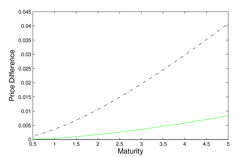
Figure 1: Option price differences against maturities. The solid line corresponds to the price difference between the default-free model and the proposed hybrid model, and the dot-dashed line corresponds to the price difference between the default-free model and the reduced-form model.
Refer to caption
Figure 2: Option price differences against strike prices. The solid line corresponds to the price difference between the default-free model and the proposed hybrid model, and the dot-dashed line corresponds to the price difference between the default-free model and the reduced-form model.
Refer to caption
Refer to caption
Figure 3: Option prices against the values of βs\beta_{s} and βv\beta_{v} . The solid, dotted and dot-dashed lines correspond to default-free option prices, option prices in the proposed hybrid model and option prices in the reduced-form model, respectively.
Refer to caption
Refer to caption
Figure 4: Option price differences against the values of βs\beta_{s} and βv\beta_{v}. The solid line corresponds to the price difference between the default-free model and the proposed hybrid model, and the dot-dashed line corresponds to the price difference between the default-free model and the reduced-form model.
Refer to caption
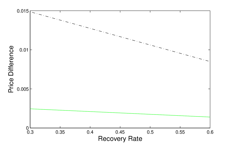
Figure 5: Option price differences against recovery rates. The solid line corresponds to the price difference between the default-free model and the proposed hybrid model, and the dot-dashed line corresponds to the price difference between the default-free model and the reduced-form model.
Refer to caption
Figure 6: Option price differences against different caused losses. The solid line corresponds to the price difference between the default-free model and the proposed hybrid model, and the dot-dashed line corresponds to the price difference between the default-free model and the reduced-form model.

Figure 1 displays the price difference with different maturities. The option prices obtained from the proposed hybrid model are close to the option prices without default risk, especially when the maturity is short. By contrast, default risk in the reduced-form model has a more pronounced effect. This is because in the reduced-form model default happens when trigger events occur, while in the hybrid model default happens only when trigger events occur and the values of the issuer’s assets at the arrival time of the trigger events are less than the losses. In other words, default happens more likely in the reduced-form model, thus reducing option prices more significantly. Figure 2 illustrates the price difference against different strike prices. A higher strike price will yield a cheaper option. Similar to Figure 1, the option has the lowest value in the reduced-form model, as it is more likely to default compared to the hybrid model.

Figure 3 shows the option values against the sensitivity parameters βs\beta_{s} and βv\beta_{v}, and the corresponding price difference is shown in Figure 4. Recall that βs\beta_{s} represents the sensitivity of the stock price against systematic risk. The option prices will increase with larger βs\beta_{s}, i.e. with larger systematic risks. Intuitively, with a larger value of βs\beta_{s}, the value of the underlying asset becomes more volatile. Thus, it is more likely the option is in-the-money and, therefore, its price becomes higher. On the other hand, since βv\beta_{v} captures the sensitivity of the issuer’s assets to systematic risk, larger βv\beta_{v} means the issuer’s assets become more risky and, as a result, the issuer is more likely to default. Therefore, one might expect the option prices in the hybrid model become smaller with larger βv\beta_{v}. However, this is not the case. We observe from Figure 3(b) a higher option price with increasing βv\beta_{v}. This is because larger βv\beta_{v} also means the underlying assets and the issuer’s assets are more likely to be correlated, which in turn makes option issuers less likely to default when call options end in the money, yielding a higher option price consequently.

Figure 5 depicts the price difference with different recovery rates. Intuitively, a higher recovery rate corresponds to a higher option price. However, the effects of recovery rates in the hybrid model are not as significant as those in the reduced-form model. Figure 6 shows the price difference with different losses (i.e. different values of LGD). The option prices without default risk and the values of options in the reduced-form model are not affected by the caused losses. In the hybrid model, it is more likely that default occurs with a higher value of losses, resulting in a lower option price and a higher default premium.

4 Conclusion

In this paper, we contribute to the literature on vulnerable options by working under a hybrid credit risk model. The proposed hybrid credit risk model incorporates the features of both structural and reduced-form models. The dynamics of the market index, as well as the dynamics of the underlying assets and option issuer’s assets are driven by Heston-Nandi GARCH processes. The underlying intensity process is exposed to both systematic risk and idiosyncratic risk. In this way, all the dynamics are correlated with each other through the systematic risk factor. Finally, we derive an explicit pricing formula of vulnerable options and perform numerical analysis to illustrate option prices.

Acknowledgement

The authors would like to thank the anonymous referee and the editor for their helpful comments and valuable suggestions that led to several important improvements. All errors are our responsibility.

Appendix

Proof of Proposition 2.1:
We first focus on the case j≤t≤Tj\leq t\leq T. Note that given the information at time tt, V⁡(j)V(j), Λ⁡(j)\Lambda(j) and ∑k=1j−1Λ⁡(k)\sum_{k=1}^{j-1}\Lambda(k) are all known. Therefore, we obtain that

f⁡(t)\displaystyle f(t) =\displaystyle= Et​[exp⁡{ϕ1​ln⁡S⁡(T)+ϕ2​ln⁡V⁡(j)+ϕ3​Λ​(j)+ϕ4​∑k=1j−1Λ⁡(k)}]\displaystyle E_{t}\Big[\exp\Big\{\phi_{1}\ln S(T)+\phi_{2}\ln V(j)+\phi_{3}\Lambda(j)+\phi_{4}\sum_{k=1}^{j-1}\Lambda(k)\Big\}\Big]
=\displaystyle= eϕ2​ln⁡V⁡(j)+ϕ3​Λ​(j)+ϕ4​∑k=1j−1Λ⁡(k)​Et​[exp⁡{ϕ1​ln⁡S⁡(T)}].\displaystyle e^{\phi_{2}\ln V(j)+\phi_{3}\Lambda(j)+\phi_{4}\sum_{k=1}^{j-1}\Lambda(k)}E_{t}\Big[\exp\Big\{\phi_{1}\ln S(T)\Big\}\Big].

In addition, at time TT, S⁡(T)S(T) is also known, it follows that

f⁡(T)\displaystyle f(T) =\displaystyle= eϕ2​ln⁡V⁡(j)+ϕ3​Λ​(j)+ϕ4​∑k=1j−1Λ⁡(k)​ET​[exp⁡{ϕ1​ln⁡S⁡(T)}]\displaystyle e^{\phi_{2}\ln V(j)+\phi_{3}\Lambda(j)+\phi_{4}\sum_{k=1}^{j-1}\Lambda(k)}E_{T}\Big[\exp\Big\{\phi_{1}\ln S(T)\Big\}\Big]
=\displaystyle= eϕ1​ln⁡S⁡(T)+ϕ2​ln⁡V⁡(j)+ϕ3​Λ​(j)+ϕ4​∑k=1j−1Λ⁡(k),\displaystyle e^{\phi_{1}\ln S(T)+\phi_{2}\ln V(j)+\phi_{3}\Lambda(j)+\phi_{4}\sum_{k=1}^{j-1}\Lambda(k)},

which in turn implies that

A0​(T)=A1​(T)=A2​(T)=0.\displaystyle A_{0}(T)=A_{1}(T)=A_{2}(T)=0.

According to the law of iterated expectations, we have that

Et​[exp⁡{ϕ1​ln⁡S⁡(T)}]\displaystyle E_{t}\Big[\exp\Big\{\phi_{1}\ln S(T)\Big\}\Big]
=\displaystyle= Et​[Et+1​[exp⁡{ϕ1​ln⁡S⁡(T)}]]\displaystyle E_{t}\Big[E_{t+1}\Big[\exp\Big\{\phi_{1}\ln S(T)\Big\}\Big]\Big]
=\displaystyle= Et​[exp⁡{ϕ1​ln⁡S⁡(t+1)+A0​(t+1)+A1​(t+1)​hm​(t+2)+A2​(t+1)​hs​(t+2)}].\displaystyle E_{t}\Big[\exp\Big\{\phi_{1}\ln S(t+1)+A_{0}(t+1)+A_{1}(t+1)h_{m}(t+2)+A_{2}(t+1)h_{s}(t+2)\Big\}\Big].

Substituting the dynamics of ln⁡S⁡(t+1)\ln S(t+1), hm​(t+2)h_{m}(t+2) and hs​(t+2)h_{s}(t+2) yields that

Et​[exp⁡{ϕ1​ln⁡S⁡(T)}]\displaystyle E_{t}\Big[\exp\Big\{\phi_{1}\ln S(T)\Big\}\Big]
=\displaystyle= Et​[exp⁡{ϕ1​ln⁡S⁡(t+1)+A0​(t+1)+A1​(t+1)​hm​(t+2)+A2​(t+1)​hs​(t+2)}]\displaystyle E_{t}\Big[\exp\Big\{\phi_{1}\ln S(t+1)+A_{0}(t+1)+A_{1}(t+1)h_{m}(t+2)+A_{2}(t+1)h_{s}(t+2)\Big\}\Big]
=\displaystyle= Et[exp{ϕ1lnS(t)+ϕ1r−12ϕ1hs(t+1)+ϕ1hs​(t+1)Zs(t+1)\displaystyle E_{t}\Big[\exp\Big\{\phi_{1}\ln S(t)+\phi_{1}r-\frac{1}{2}\phi_{1}h_{s}(t+1)+\phi_{1}\sqrt{h_{s}(t+1)}Z_{s}(t+1)
−12​ϕ1​βs2​hm​(t+1)+ϕ1​βs​hm​(t+1)​Zm​(t+1)+A0​(t+1)\displaystyle\ \ \ \ \ \ \ \ \ \ -\frac{1}{2}\phi_{1}\beta_{s}^{2}h_{m}(t+1)+\phi_{1}\beta_{s}\sqrt{h_{m}(t+1)}Z_{m}(t+1)+A_{0}(t+1)
+A1​(t+1)​(wm+bm​hm​(t+1)+am​(Zm​(t+1)−cm​hm​(t+1))2)\displaystyle+A_{1}(t+1)\Big(w_{m}+b_{m}h_{m}(t+1)+a_{m}(Z_{m}(t+1)-c_{m}\sqrt{h_{m}(t+1)})^{2}\Big)
+A2(t+1)(ws+bshs(t+1)+as(Zs(t+1)−cshs​(t+1))2)}].\displaystyle+A_{2}(t+1)\Big(w_{s}+b_{s}h_{s}(t+1)+a_{s}(Z_{s}(t+1)-c_{s}\sqrt{h_{s}(t+1)})^{2}\Big)\Big\}\Big].

Using the fact that E​ea​(Z+b)2=e−12​ln⁡(1−2​a)+a​b21−2​aEe^{a(Z+b)^{2}}=e^{-\frac{1}{2}\ln(1-2a)+\frac{ab^{2}}{1-2a}} with ZZ being a standard normal variable and some algebra shows that

A0​(t)=\displaystyle A_{0}(t)= ϕ1​r+A0​(t+1)+wm​A1​(t+1)+ws​A2​(t+1)−12​ln⁡(1−2​am​A1​(t+1))\displaystyle\phi_{1}r+A_{0}(t+1)+w_{m}A_{1}(t+1)+w_{s}A_{2}(t+1)-\frac{1}{2}\ln(1-2a_{m}A_{1}(t+1))
−12​ln⁡(1−2​as​A2​(t+1)),\displaystyle-\frac{1}{2}\ln(1-2a_{s}A_{2}(t+1)),
A1​(t)=\displaystyle A_{1}(t)= bm​A1​(t+1)−12​ϕ1​βs2+ϕ1​βs​cm−12​cm2+12​(ϕ1​βs−cm)21−2​am​A1​(t+1),\displaystyle b_{m}A_{1}(t+1)-\frac{1}{2}\phi_{1}\beta_{s}^{2}+\phi_{1}\beta_{s}c_{m}-\frac{1}{2}c_{m}^{2}+\frac{\frac{1}{2}(\phi_{1}\beta_{s}-c_{m})^{2}}{1-2a_{m}A_{1}(t+1)},
A2​(t)=\displaystyle A_{2}(t)= bs​A2​(t+1)−12​ϕ1+ϕ1​cs−12​cs2+12​(ϕ1−cs)21−2​as​A2​(t+1).\displaystyle b_{s}A_{2}(t+1)-\frac{1}{2}\phi_{1}+\phi_{1}c_{s}-\frac{1}{2}c_{s}^{2}+\frac{\frac{1}{2}(\phi_{1}-c_{s})^{2}}{1-2a_{s}A_{2}(t+1)}.

Hence, A0​(t)A_{0}(t), A1​(t)A_{1}(t) and A2​(t)A_{2}(t) (j≤t≤Tj\leq t\leq T) can be obtained recursively with terminal conditions A0​(T)=A1​(T)=A2​(T)=0A_{0}(T)=A_{1}(T)=A_{2}(T)=0 and the above expressions.

In what follows, we turn to the case t<jt<j. Applying the law of iterated expectations to f⁡(t)f(t) yields that

f⁡(t)\displaystyle f(t) =\displaystyle= Et​[exp⁡{ϕ1​ln⁡S⁡(T)+ϕ2​ln⁡V⁡(j)+ϕ3​Λ​(j)+ϕ4​∑k=1j−1Λ⁡(k)}]\displaystyle E_{t}\Big[\exp\Big\{\phi_{1}\ln S(T)+\phi_{2}\ln V(j)+\phi_{3}\Lambda(j)+\phi_{4}\sum_{k=1}^{j-1}\Lambda(k)\Big\}\Big]
=\displaystyle= Et​[Et+1​[exp⁡{ϕ1​ln⁡S⁡(T)+ϕ2​ln⁡V⁡(j)+ϕ3​Λ​(j)+ϕ4​∑k=1j−1Λ⁡(k)}]]\displaystyle E_{t}\Big[E_{t+1}\Big[\exp\Big\{\phi_{1}\ln S(T)+\phi_{2}\ln V(j)+\phi_{3}\Lambda(j)+\phi_{4}\sum_{k=1}^{j-1}\Lambda(k)\Big\}\Big]\Big]
=\displaystyle= Et​[f​(t+1)]\displaystyle E_{t}\Big[f(t+1)\Big]
=\displaystyle= Et[exp{ϕ2lnV(t+1)+ϕ4∑k=1t+1Λ(k)+ϕ1lnS(t+1)+B0(t+1)\displaystyle E_{t}\Big[\exp\Big\{\phi_{2}\ln V(t+1)+\phi_{4}\sum_{k=1}^{t+1}\Lambda(k)+\phi_{1}\ln S(t+1)+B_{0}(t+1)
+B1(t+1)hm(t+2)+B2(t+1)hs(t+2)+B3(t+1)hv(t+2)+B4(t+1)Λ(t+2)}].\displaystyle\ \ \ \ +B_{1}(t+1)h_{m}(t+2)+B_{2}(t+1)h_{s}(t+2)+B_{3}(t+1)h_{v}(t+2)+B_{4}(t+1)\Lambda(t+2)\Big\}\Big].

Substituting the dynamics of ln⁡V⁡(t+1)\ln V(t+1), Λ⁡(t+2)\Lambda(t+2), ln⁡S⁡(t+1)\ln S(t+1), hm​(t+2)h_{m}(t+2), hs​(t+2)h_{s}(t+2) and hv​(t+2)h_{v}(t+2) yields that

f⁡(t)\displaystyle f(t) =\displaystyle= Et[exp{ϕ2lnV(t+1)+ϕ4∑k=1t+1Λ(k)+ϕ1lnS(t+1)+B0(t+1)\displaystyle E_{t}\Big[\exp\Big\{\phi_{2}\ln V(t+1)+\phi_{4}\sum_{k=1}^{t+1}\Lambda(k)+\phi_{1}\ln S(t+1)+B_{0}(t+1)
+B1(t+1)hm(t+2)+B2(t+1)hs(t+2)+B3(t+1)hv(t+2)+B4(t+1)Λ(t+2)}]\displaystyle\ \ \ \ +B_{1}(t+1)h_{m}(t+2)+B_{2}(t+1)h_{s}(t+2)+B_{3}(t+1)h_{v}(t+2)+B_{4}(t+1)\Lambda(t+2)\Big\}\Big]
=\displaystyle= Et[exp{ϕ2lnV(t)+ϕ2r−12ϕ2hv(t+1)+ϕ2hv​(t+1)Zv(t+1)\displaystyle E_{t}\Big[\exp\Big\{\phi_{2}\ln V(t)+\phi_{2}r-\frac{1}{2}\phi_{2}h_{v}(t+1)+\phi_{2}\sqrt{h_{v}(t+1)}Z_{v}(t+1)
−12​ϕ2​βv2​hm​(t+1)+ϕ2​βv​hm​(t+1)​Zm​(t+1)+ϕ4​∑k=1t+1Λ⁡(k)\displaystyle\ \ \ \ \ \ \ \ \ \ -\frac{1}{2}\phi_{2}\beta_{v}^{2}h_{m}(t+1)+\phi_{2}\beta_{v}\sqrt{h_{m}(t+1)}Z_{m}(t+1)+\phi_{4}\sum_{k=1}^{t+1}\Lambda(k)
+ϕ1​ln⁡S⁡(t)+ϕ1​r−12​ϕ1​hs​(t+1)+ϕ1​hs​(t+1)​Zs​(t+1)\displaystyle\ \ \ \ \ \ \ \ \ \ +\phi_{1}\ln S(t)+\phi_{1}r-\frac{1}{2}\phi_{1}h_{s}(t+1)+\phi_{1}\sqrt{h_{s}(t+1)}Z_{s}(t+1)
−12​ϕ1​βs2​hm​(t+1)+ϕ1​βs​hm​(t+1)​Zm​(t+1)+B0​(t+1)\displaystyle\ \ \ \ \ \ \ \ \ \ -\frac{1}{2}\phi_{1}\beta_{s}^{2}h_{m}(t+1)+\phi_{1}\beta_{s}\sqrt{h_{m}(t+1)}Z_{m}(t+1)+B_{0}(t+1)
+B1​(t+1)​(wm+bm​hm​(t+1)+am​(Zm​(t+1)−cm​hm​(t+1))2)\displaystyle\ \ \ \ \ \ \ \ \ \ +B_{1}(t+1)\Big(w_{m}+b_{m}h_{m}(t+1)+a_{m}(Z_{m}(t+1)-c_{m}\sqrt{h_{m}(t+1)})^{2}\Big)
+B2​(t+1)​(ws+bs​hs​(t+1)+as​(Zs​(t+1)−cs​hs​(t+1))2)\displaystyle\ \ \ \ \ \ \ \ \ \ +B_{2}(t+1)\Big(w_{s}+b_{s}h_{s}(t+1)+a_{s}(Z_{s}(t+1)-c_{s}\sqrt{h_{s}(t+1)})^{2}\Big)
+B3​(t+1)​(wv+bv​hv​(t+1)+av​(Zv​(t+1)−cv​hv​(t+1))2)\displaystyle\ \ \ \ \ \ \ \ \ \ +B_{3}(t+1)\Big(w_{v}+b_{v}h_{v}(t+1)+a_{v}(Z_{v}(t+1)-c_{v}\sqrt{h_{v}(t+1)})^{2}\Big)
+B4(t+1)(wλ+bλΛ(t+1)+aλ(Zm(t+1))2+cλ(Zv(t+1))2)}].\displaystyle\ \ \ \ \ \ \ \ \ \ +B_{4}(t+1)\Big(w_{\lambda}+b_{\lambda}\Lambda(t+1)+a_{\lambda}(Z_{m}(t+1))^{2}+c_{\lambda}(Z_{v}(t+1))^{2}\Big)\Big\}\Big].

Rearranging terms implies that

f⁡(t)\displaystyle f(t) =\displaystyle= Et[exp{ϕ2lnV(t)+ϕ4∑k=1tΛ(k)+ϕ1lnS(t)+B0(t+1)+(ϕ2+ϕ1)r\displaystyle E_{t}\Big[\exp\Big\{\phi_{2}\ln V(t)+\phi_{4}\sum_{k=1}^{t}\Lambda(k)+\phi_{1}\ln S(t)+B_{0}(t+1)+(\phi_{2}+\phi_{1})r
+wm​B1​(t+1)+ws​B2​(t+1)+wv​B3​(t+1)+wλ​B4​(t+1)\displaystyle\ \ \ \ \ \ \ \ \ \ +w_{m}B_{1}(t+1)+w_{s}B_{2}(t+1)+w_{v}B_{3}(t+1)+w_{\lambda}B_{4}(t+1)
+(bm​B1​(t+1)−12​ϕ2​βv2−12​ϕ1​βs2)​hm​(t+1)\displaystyle\ \ \ \ \ \ \ \ \ \ +(b_{m}B_{1}(t+1)-\frac{1}{2}\phi_{2}\beta_{v}^{2}-\frac{1}{2}\phi_{1}\beta_{s}^{2})h_{m}(t+1)
+(bv​B3​(t+1)−12​ϕ2)​hv​(t+1)+(bs​B2​(t+1)−12​ϕ1)​hs​(t+1)\displaystyle\ \ \ \ \ \ \ \ \ \ +(b_{v}B_{3}(t+1)-\frac{1}{2}\phi_{2})h_{v}(t+1)+(b_{s}B_{2}(t+1)-\frac{1}{2}\phi_{1})h_{s}(t+1)
+(bλB4(t+1)+ϕ4)Λ(t+1)+Φm+Φs+Φv}],\displaystyle\ \ \ \ \ \ \ \ \ \ +(b_{\lambda}B_{4}(t+1)+\phi_{4})\Lambda(t+1)+\Phi_{m}+\Phi_{s}+\Phi_{v}\Big\}\Big],

where

Φs\displaystyle\Phi_{s} =\displaystyle= ϕ1​hs​(t+1)​Zs​(t+1)+as​B2​(t+1)​(Zs​(t+1)−cs​hs​(t+1))2,\displaystyle\phi_{1}\sqrt{h_{s}(t+1)}Z_{s}(t+1)+a_{s}B_{2}(t+1)(Z_{s}(t+1)-c_{s}\sqrt{h_{s}(t+1)})^{2},
Φv\displaystyle\Phi_{v} =\displaystyle= ϕ2​hv​(t+1)​Zv​(t+1)+av​B3​(t+1)​(Zv​(t+1)−cv​hv​(t+1))2\displaystyle\phi_{2}\sqrt{h_{v}(t+1)}Z_{v}(t+1)+a_{v}B_{3}(t+1)(Z_{v}(t+1)-c_{v}\sqrt{h_{v}(t+1)})^{2}
+cλ​B4​(t+1)​(Zv​(t+1))2,\displaystyle\ \ \ \ \ \ \ \ \ \ +c_{\lambda}B_{4}(t+1)(Z_{v}(t+1))^{2},
Φm\displaystyle\Phi_{m} =\displaystyle= (ϕ2​βv+ϕ1​βs)​hm​(t+1)​Zm​(t+1)+am​B1​(t+1)​(Zm​(t+1)−cm​hm​(t+1))2\displaystyle(\phi_{2}\beta_{v}+\phi_{1}\beta_{s})\sqrt{h_{m}(t+1)}Z_{m}(t+1)+a_{m}B_{1}(t+1)(Z_{m}(t+1)-c_{m}\sqrt{h_{m}(t+1)})^{2}
+aλ​B4​(t+1)​(Zm​(t+1))2.\displaystyle\ \ \ \ \ \ \ \ \ \ +a_{\lambda}B_{4}(t+1)(Z_{m}(t+1))^{2}.

In order to obtain the explicit expression of f⁡(t)f(t), we only need to calculate Et​[eΦm+Φs+Φv]=Et​[eΦm]​Et​[eΦs]​Et​[eΦv]E_{t}[e^{\Phi_{m}+\Phi_{s}+\Phi_{v}}]=E_{t}[e^{\Phi_{m}}]E_{t}[e^{\Phi_{s}}]E_{t}[e^{\Phi_{v}}]. Note that Φs\Phi_{s}, Φm\Phi_{m} and Φv\Phi_{v} have similar forms and all can be obtained based on the following form,

E⁡[exp⁡{μ1​h​Z+μ2​(Z−μ3​h)2+μ4​Z2}],\displaystyle E[\exp\{\mu_{1}\sqrt{h}Z+\mu_{2}(Z-\mu_{3}\sqrt{h})^{2}+\mu_{4}Z^{2}\}],

where μ1\mu_{1}, μ2\mu_{2}, μ3\mu_{3} and μ4\mu_{4} are all constants and ZZ is a standard normal variable. Using the fact that E​ea​(Z+b)2=e−12​ln⁡(1−2​a)+a​b21−2​aEe^{a(Z+b)^{2}}=e^{-\frac{1}{2}\ln(1-2a)+\frac{ab^{2}}{1-2a}}, we have that

E⁡[exp⁡{μ1​h​Z+μ2​(Z−μ3​h)2+μ4​Z2}]\displaystyle E[\exp\{\mu_{1}\sqrt{h}Z+\mu_{2}(Z-\mu_{3}\sqrt{h})^{2}+\mu_{4}Z^{2}\}] (A.1)
=\displaystyle= E⁡[exp⁡{(μ2+μ4)​Z2−2​(μ2​μ3−μ1/2)​Z​h+μ2​μ32​h}]\displaystyle E[\exp\{(\mu_{2}+\mu_{4})Z^{2}-2(\mu_{2}\mu_{3}-\mu_{1}/2)Z\sqrt{h}+\mu_{2}\mu_{3}^{2}h\}]
=\displaystyle= E⁡[exp⁡{(μ2+μ4)​(Z−μ2​μ3−μ1/2μ2+μ4​h)2−(μ2​μ3−μ1/2)2μ2+μ4​h+μ2​μ32​h}]\displaystyle E[\exp\{(\mu_{2}+\mu_{4})\Big(Z-\frac{\mu_{2}\mu_{3}-\mu_{1}/2}{\mu_{2}+\mu_{4}}\sqrt{h}\Big)^{2}-\frac{(\mu_{2}\mu_{3}-\mu_{1}/2)^{2}}{\mu_{2}+\mu_{4}}h+\mu_{2}\mu_{3}^{2}h\}]
=\displaystyle= eμ2​μ32​h−(μ2​μ3−μ1/2)2μ2+μ4​h​E​[exp⁡{(μ2+μ4)​(Z−μ2​μ3−μ1/2μ2+μ4​h)2}]\displaystyle e^{\mu_{2}\mu_{3}^{2}h-\frac{(\mu_{2}\mu_{3}-\mu_{1}/2)^{2}}{\mu_{2}+\mu_{4}}h}E[\exp\{(\mu_{2}+\mu_{4})\Big(Z-\frac{\mu_{2}\mu_{3}-\mu_{1}/2}{\mu_{2}+\mu_{4}}\sqrt{h}\Big)^{2}\}]
=\displaystyle= exp⁡{μ2​μ32​h−(μ2​μ3−μ1/2)2μ2+μ4​h−12​ln⁡(1−2​(μ2+μ4))+(μ2+μ4)​(μ2​μ3−μ1/2μ2+μ4)21−2​(μ2+μ4)​h}\displaystyle\exp\{\mu_{2}\mu_{3}^{2}h-\frac{(\mu_{2}\mu_{3}-\mu_{1}/2)^{2}}{\mu_{2}+\mu_{4}}h-\frac{1}{2}\ln(1-2(\mu_{2}+\mu_{4}))+\frac{(\mu_{2}+\mu_{4})(\frac{\mu_{2}\mu_{3}-\mu_{1}/2}{\mu_{2}+\mu_{4}})^{2}}{1-2(\mu_{2}+\mu_{4})}h\}
=\displaystyle= exp⁡{−12​ln⁡(1−2​(μ2+μ4))+(μ2​μ32−(μ2​μ3−μ1/2)2μ2+μ4+(μ2+μ4)​(μ2​μ3−μ1/2μ2+μ4)21−2​(μ2+μ4))​h}\displaystyle\exp\{-\frac{1}{2}\ln(1-2(\mu_{2}+\mu_{4}))+\Big(\mu_{2}\mu_{3}^{2}-\frac{(\mu_{2}\mu_{3}-\mu_{1}/2)^{2}}{\mu_{2}+\mu_{4}}+\frac{(\mu_{2}+\mu_{4})(\frac{\mu_{2}\mu_{3}-\mu_{1}/2}{\mu_{2}+\mu_{4}})^{2}}{1-2(\mu_{2}+\mu_{4})}\Big)h\}
=\displaystyle= exp⁡{−12​ln⁡(1−2​(μ2+μ4))+(μ2​μ32+2​(μ2​μ3−μ1/2)21−2​(μ2+μ4))​h}.\displaystyle\exp\{-\frac{1}{2}\ln(1-2(\mu_{2}+\mu_{4}))+\Big(\mu_{2}\mu_{3}^{2}+\frac{2(\mu_{2}\mu_{3}-\mu_{1}/2)^{2}}{1-2(\mu_{2}+\mu_{4})}\Big)h\}.

Therefore, we can write f⁡(t)f(t) in the following form

f⁡(t)\displaystyle f(t) =\displaystyle= exp{ϕ2lnV(t)+ϕ4∑k=1tΛ(k)+ϕ1lnS(t)+B0(t)\displaystyle\exp\Big\{\phi_{2}\ln V(t)+\phi_{4}\sum_{k=1}^{t}\Lambda(k)+\phi_{1}\ln S(t)+B_{0}(t)
+B1(t)hm(t+1)+B2(t)hs(t+1)+B3(t)hv(t+1)+B4(t+1)Λ(t+1)},\displaystyle\ \ \ \ \ \ \ \ \ \ \ +B_{1}(t)h_{m}(t+1)+B_{2}(t)h_{s}(t+1)+B_{3}(t)h_{v}(t+1)+B_{4}(t+1)\Lambda(t+1)\Big\},

where

B0​(t)\displaystyle B_{0}(t) =\displaystyle= B0​(t+1)+(ϕ2+ϕ1)​r+wm​B1​(t+1)+ws​B2​(t+1)+wv​B3​(t+1)+wλ​B4​(t+1)\displaystyle B_{0}(t+1)+(\phi_{2}+\phi_{1})r+w_{m}B_{1}(t+1)+w_{s}B_{2}(t+1)+w_{v}B_{3}(t+1)+w_{\lambda}B_{4}(t+1)
OPEN−12​ln⁡(1−2​(am​B1​(t+1)+aλ​B4​(t+1)))−12​ln⁡(1−2​as​B2​(t+1)))\displaystyle\ \ \ -\frac{1}{2}\ln(1-2(a_{m}B_{1}(t+1)+a_{\lambda}B_{4}(t+1)))-\frac{1}{2}\ln(1-2a_{s}B_{2}(t+1)))
−12​ln⁡(1−2​(av​B3​(t+1)+cλ​B4​(t+1))),\displaystyle\ \ \ -\frac{1}{2}\ln(1-2(a_{v}B_{3}(t+1)+c_{\lambda}B_{4}(t+1))),
B1​(t)\displaystyle B_{1}(t) =\displaystyle= bm​B1​(t+1)−12​ϕ2​βv2−12​ϕ1​βs2+am​cm2​B1​(t+1)\displaystyle b_{m}B_{1}(t+1)-\frac{1}{2}\phi_{2}\beta_{v}^{2}-\frac{1}{2}\phi_{1}\beta_{s}^{2}+a_{m}c_{m}^{2}B_{1}(t+1)
+2​(am​cm​B1​(t+1)−(ϕ2​βv+ϕ1​βs)/2)21−2​(am​B1​(t+1)+aλ​B4​(t+1)),\displaystyle\ \ \ +\frac{2(a_{m}c_{m}B_{1}(t+1)-(\phi_{2}\beta_{v}+\phi_{1}\beta_{s})/2)^{2}}{1-2(a_{m}B_{1}(t+1)+a_{\lambda}B_{4}(t+1))},
B2​(t)\displaystyle B_{2}(t) =\displaystyle= bs​B2​(t+1)−12​ϕ1+as​cs2​B2​(t+1)+2​(as​cs​B2​(t+1)−ϕ1/2)21−2​as​B2​(t+1),\displaystyle b_{s}B_{2}(t+1)-\frac{1}{2}\phi_{1}+a_{s}c_{s}^{2}B_{2}(t+1)+\frac{2(a_{s}c_{s}B_{2}(t+1)-\phi_{1}/2)^{2}}{1-2a_{s}B_{2}(t+1)},
B3​(t)\displaystyle B_{3}(t) =\displaystyle= bv​B3​(t+1)−12​ϕ2+av​cv2​B3​(t+1)+2​(av​cv​B3​(t+1)−ϕ2/2)21−2​(av​B3​(t+1)+cλ​B4​(t+1)),\displaystyle b_{v}B_{3}(t+1)-\frac{1}{2}\phi_{2}+a_{v}c_{v}^{2}B_{3}(t+1)+\frac{2(a_{v}c_{v}B_{3}(t+1)-\phi_{2}/2)^{2}}{1-2(a_{v}B_{3}(t+1)+c_{\lambda}B_{4}(t+1))},
B4​(t)\displaystyle B_{4}(t) =\displaystyle= bλ​B4​(t+1)+ϕ4.\displaystyle b_{\lambda}B_{4}(t+1)+\phi_{4}.

Now we need the terminal conditions of Bk​(t),k=0,1,2,3,4B_{k}(t),\ k=0,1,2,3,4 (t<jt<j). In other words, we need to determine the values of Bk​(j−1),k=0,1,2,3,4B_{k}(j-1),\ k=0,1,2,3,4. Actually, we already have the expression of f⁡(j)f(j) from the case j≤t≤Tj\leq t\leq T we previously considered,

f⁡(j)\displaystyle f(j) =\displaystyle= exp{ϕ2lnV(j)+ϕ3Λ(j)+ϕ4∑k=1j−1Λ(k)+ϕ1lnS(j)+A0(j)\displaystyle\exp\Big\{\phi_{2}\ln V(j)+\phi_{3}\Lambda(j)+\phi_{4}\sum_{k=1}^{j-1}\Lambda(k)+\phi_{1}\ln S(j)+A_{0}(j)
+A1(j)hm(j+1)+A2(j)hs(j+1)}.\displaystyle\ \ \ \ \ \ \ \ \ \ \ +A_{1}(j)h_{m}(j+1)+A_{2}(j)h_{s}(j+1)\Big\}.

According to the law of iterated expectations, we have that

f⁡(j−1)\displaystyle f(j-1) =\displaystyle= Ej−1​[f​(j)]\displaystyle E_{j-1}\Big[f(j)\Big]
=\displaystyle= Ej−1[exp{ϕ2lnV(j)+ϕ3Λ(j)+ϕ4∑k=1j−1Λ(k)+ϕ1lnS(j)+A0(j)\displaystyle E_{j-1}\Big[\exp\Big\{\phi_{2}\ln V(j)+\phi_{3}\Lambda(j)+\phi_{4}\sum_{k=1}^{j-1}\Lambda(k)+\phi_{1}\ln S(j)+A_{0}(j)
+A1(j)hm(j+1)+A2(j)hs(j+1)}].\displaystyle\ \ \ \ \ \ \ \ \ \ \ +A_{1}(j)h_{m}(j+1)+A_{2}(j)h_{s}(j+1)\Big\}\Big].

Substituting the dynamics of ln⁡V⁡(j)\ln V(j), ln⁡S⁡(j)\ln S(j), hm​(j+1)h_{m}(j+1), and hs​(j+1)h_{s}(j+1) and using (A.1) imply that

f⁡(j−1)\displaystyle f(j-1) =\displaystyle= Ej−1[exp{ϕ2lnV(j)+ϕ3Λ(j)+ϕ4∑k=1j−1Λ(k)+ϕ1lnS(j)+A0(j)\displaystyle E_{j-1}\Big[\exp\Big\{\phi_{2}\ln V(j)+\phi_{3}\Lambda(j)+\phi_{4}\sum_{k=1}^{j-1}\Lambda(k)+\phi_{1}\ln S(j)+A_{0}(j)
+A1(j)hm(j+1)+A2(j)hs(j+1)}]\displaystyle\ \ \ \ \ \ \ \ \ \ \ +A_{1}(j)h_{m}(j+1)+A_{2}(j)h_{s}(j+1)\Big\}\Big]
=\displaystyle= Et[exp{ϕ2lnV(j−1)+ϕ2r−12ϕ2hv(j)+ϕ2hv​(j)Zv(j)\displaystyle E_{t}\Big[\exp\Big\{\phi_{2}\ln V(j-1)+\phi_{2}r-\frac{1}{2}\phi_{2}h_{v}(j)+\phi_{2}\sqrt{h_{v}(j)}Z_{v}(j)
−12​ϕ2​βv2​hm​(j)+ϕ2​βv​hm​(j)​Zm​(j)+ϕ3​Λ​(j)+ϕ4​∑k=1j−1Λ⁡(k)\displaystyle\ \ \ \ \ \ \ \ \ \ -\frac{1}{2}\phi_{2}\beta_{v}^{2}h_{m}(j)+\phi_{2}\beta_{v}\sqrt{h_{m}(j)}Z_{m}(j)+\phi_{3}\Lambda(j)+\phi_{4}\sum_{k=1}^{j-1}\Lambda(k)
+ϕ1​ln⁡S⁡(j−1)+ϕ1​r−12​ϕ1​hs​(j)+ϕ1​hs​(j)​Zs​(j)\displaystyle\ \ \ \ \ \ \ \ \ \ +\phi_{1}\ln S(j-1)+\phi_{1}r-\frac{1}{2}\phi_{1}h_{s}(j)+\phi_{1}\sqrt{h_{s}(j)}Z_{s}(j)
−12​ϕ1​βs2​hm​(j)+ϕ1​βs​hm​(j)​Zm​(j)+A0​(j)\displaystyle\ \ \ \ \ \ \ \ \ \ -\frac{1}{2}\phi_{1}\beta_{s}^{2}h_{m}(j)+\phi_{1}\beta_{s}\sqrt{h_{m}(j)}Z_{m}(j)+A_{0}(j)
+A1​(j)​(wm+bm​hm​(j)+am​(Zm​(j)−cm​hm​(j))2)\displaystyle\ \ \ \ \ \ \ \ \ \ +A_{1}(j)\Big(w_{m}+b_{m}h_{m}(j)+a_{m}(Z_{m}(j)-c_{m}\sqrt{h_{m}(j)})^{2}\Big)
+A2(j)(ws+bshs(j)+as(Zs(j)−cshs​(j))2)}]\displaystyle\ \ \ \ \ \ \ \ \ \ +A_{2}(j)\Big(w_{s}+b_{s}h_{s}(j)+a_{s}(Z_{s}(j)-c_{s}\sqrt{h_{s}(j)})^{2}\Big)\Big\}\Big]
=\displaystyle= exp{ϕ2lnV(j−1)+ϕ4∑k=1j−1Λ(k)+ϕ1lnS(j−1)+B0(j−1)\displaystyle\exp\Big\{\phi_{2}\ln V(j-1)+\phi_{4}\sum_{k=1}^{j-1}\Lambda(k)+\phi_{1}\ln S(j-1)+B_{0}(j-1)
+B1(j−1)hm(j)+B2(j−1)hs(j)+B3(j−1)hv(j)+B4(j−1)Λ(j)},\displaystyle\ \ \ \ \ \ \ \ \ \ \ +B_{1}(j-1)h_{m}(j)+B_{2}(j-1)h_{s}(j)+B_{3}(j-1)h_{v}(j)+B_{4}(j-1)\Lambda(j)\Big\},

where

B0​(j−1)\displaystyle B_{0}(j-1) =\displaystyle= A0​(j)+(ϕ2+ϕ1)​r+wm​A1​(j)+ws​A2​(j)\displaystyle A_{0}(j)+(\phi_{2}+\phi_{1})r+w_{m}A_{1}(j)+w_{s}A_{2}(j)
−12​ln⁡(1−2​am​A1​(j))−12​ln⁡(1−2​as​A2​(j)),\displaystyle-\frac{1}{2}\ln(1-2a_{m}A_{1}(j))-\frac{1}{2}\ln(1-2a_{s}A_{2}(j)),
B1​(j−1)\displaystyle B_{1}(j-1) =\displaystyle= bm​A1​(j)−12​ϕ2​βv2−12​ϕ1​βs2+am​cm2​A1​(j)+2​(am​cm​A1​(j)−(ϕ2​βv+ϕ1​βs)/2)21−2​am​A1​(j),\displaystyle b_{m}A_{1}(j)-\frac{1}{2}\phi_{2}\beta_{v}^{2}-\frac{1}{2}\phi_{1}\beta_{s}^{2}+a_{m}c_{m}^{2}A_{1}(j)+\frac{2(a_{m}c_{m}A_{1}(j)-(\phi_{2}\beta_{v}+\phi_{1}\beta_{s})/2)^{2}}{1-2a_{m}A_{1}(j)},
B2​(j−1)\displaystyle B_{2}(j-1) =\displaystyle= bs​A2​(j)−12​ϕ1+as​cs2​A2​(j)+2​(as​cs​A2​(j)−ϕ1/2)21−2​as​A2​(j),\displaystyle b_{s}A_{2}(j)-\frac{1}{2}\phi_{1}+a_{s}c_{s}^{2}A_{2}(j)+\frac{2(a_{s}c_{s}A_{2}(j)-\phi_{1}/2)^{2}}{1-2a_{s}A_{2}(j)},
B3​(j−1)\displaystyle B_{3}(j-1) =\displaystyle= −12​ϕ2+12​ϕ22,\displaystyle-\frac{1}{2}\phi_{2}+\frac{1}{2}\phi_{2}^{2},
B4​(j−1)\displaystyle B_{4}(j-1) =\displaystyle= ϕ3.\displaystyle\phi_{3}.

This completes the proof of the proposition. □\Box

Proof of Theorem 2.2:
First, we deal with the term E⁡[(S⁡(T)−K)+]E\Big[(S(T)-K)^{+}\Big]. Recall the definition of f⁡(t,ϕ1,ϕ2,ϕ3,ϕ4)f(t;\phi_{1},\phi_{2},\phi_{3},\phi_{4}) and note that f⁡(0,i​ϕ1,0,0,0)f(0;i\phi_{1},0,0,0) is the characteristic function of ln⁡S⁡(T)\ln S(T) under QQ. From standard probability theory (see, e.g., Kendall and Stuart (1977)), we can obtain the distribution function of ln⁡S⁡(T)\ln S(T), that is,

Q⁡(ln⁡S⁡(T)≤x)=12−1π​∫0∞Re​[e−i​ϕ1​x​f​(0,i​ϕ1,0,0,0)i​ϕ1]​d​ϕ1,Q(\ln S(T)\leq x)=\frac{1}{2}-\frac{1}{\pi}\int_{0}^{\infty}\textrm{Re}\Big[\frac{e^{-i\phi_{1}x}f(0;i\phi_{1},0,0,0)}{i\phi_{1}}\Big]{\mathrm{d}}\phi_{1},

which in turn implies that

Q⁡(ln⁡S⁡(T)≥x)\displaystyle Q(\ln S(T)\geq x) =\displaystyle= 1−Q⁡(ln⁡S⁡(T)≤x)\displaystyle 1-Q(\ln S(T)\leq x) (A.2)
=\displaystyle= 12+1π​∫0∞Re​[e−i​ϕ1​x​f​(0,i​ϕ1,0,0,0)i​ϕ1]​d​ϕ1.\displaystyle\frac{1}{2}+\frac{1}{\pi}\int_{0}^{\infty}\textrm{Re}\Big[\frac{e^{-i\phi_{1}x}f(0;i\phi_{1},0,0,0)}{i\phi_{1}}\Big]{\mathrm{d}}\phi_{1}.

The term E⁡[(S⁡(T)−K)+]E\Big[(S(T)-K)^{+}\Big] can be derived after introducing a new probability measure Q1Q_{1} defined by

Q1​(O)=E⁡[I⁡(O)​S​(T)]E⁡[S⁡(T)],\displaystyle Q_{1}(O)=\frac{E\Big[I(O)S(T)\Big]}{E\Big[S(T)\Big]},

for any event O∈ℱTO\in\mathscr{F}_{T}. Obviously, the characteristic function of ln⁡S⁡(T)\ln S(T) under Q1Q_{1} is given by

EQ1​[ei​ϕ1​ln⁡S​(T)]\displaystyle E^{Q_{1}}\Big[e^{i\phi_{1}\ln S(T)}\Big] =\displaystyle= f⁡(0,1+i​ϕ1,0,0,0)f⁡(0,1,0,0,0).\displaystyle\frac{f(0;1+i\phi_{1},0,0,0)}{f(0;1,0,0,0)}.

In addition, under Q1Q_{1}, it holds that

Q1​(ln⁡S⁡(T)≥x)\displaystyle Q_{1}(\ln S(T)\geq x) =\displaystyle= 12+1π​∫0∞Re​[e−i​ϕ1​x​f​(0,1+i​ϕ1,0,0,0)/f⁡(0,1,0,0,0)i​ϕ1]​d​ϕ1.\displaystyle\frac{1}{2}+\frac{1}{\pi}\int_{0}^{\infty}\textrm{Re}\Big[\frac{e^{-i\phi_{1}x}f(0;1+i\phi_{1},0,0,0)/f(0;1,0,0,0)}{i\phi_{1}}\Big]{\mathrm{d}}\phi_{1}. (A.3)

Hence, (A.2) and (A.3) imply that

E⁡[(S⁡(T)−K)+]\displaystyle E\Big[(S(T)-K)^{+}\Big] =\displaystyle= E⁡[(S⁡(T)−K)+]\displaystyle E\Big[(S(T)-K)^{+}\Big] (A.4)
=\displaystyle= E⁡[(S⁡(T)−K)​I​(ln⁡S⁡(T)≥ln⁡K)]\displaystyle E\Big[(S(T)-K)I(\ln S(T)\geq\ln K)\Big]
=\displaystyle= E⁡[S⁡(T)​I​(ln⁡S⁡(T)≥ln⁡K)]−K​E​[I⁡(ln⁡S⁡(T)≥ln⁡K)]\displaystyle E\Big[S(T)I(\ln S(T)\geq\ln K)\Big]-KE\Big[I(\ln S(T)\geq\ln K)\Big]
=\displaystyle= E⁡[S⁡(T)]​EQ1​[I⁡(ln⁡S⁡(T)≥ln⁡K)]−K​E​[I⁡(ln⁡S⁡(T)≥ln⁡K)]\displaystyle E[S(T)]E^{Q_{1}}\Big[I(\ln S(T)\geq\ln K)\Big]-KE\Big[I(\ln S(T)\geq\ln K)\Big]
=\displaystyle= OPENE⁡[S⁡(T)]​Q1​(ln⁡S⁡(T)≥ln⁡K)−K​Q​(ln⁡S⁡(T)≥ln⁡K))\displaystyle E[S(T)]Q_{1}(\ln S(T)\geq\ln K)-KQ(\ln S(T)\geq\ln K)\Big)
=\displaystyle= 12​f​(0,1,0,0,0)+1π​∫0∞Re​[e−i​ϕ1​ln⁡K​f​(0,1+i​ϕ1,0,0,0)i​ϕ1]​d​ϕ1\displaystyle\frac{1}{2}f(0;1,0,0,0)+\frac{1}{\pi}\int_{0}^{\infty}\textrm{Re}\Big[\frac{e^{-i\phi_{1}\ln K}f(0;1+i\phi_{1},0,0,0)}{i\phi_{1}}\Big]{\mathrm{d}}\phi_{1}
−K2−Kπ​∫0∞Re​[e−i​ϕ1​ln⁡K​f​(0,i​ϕ1,0,0,0)i​ϕ1]​d​ϕ1,\displaystyle\ \ \ \ \ \ \ \ \ \ \ \ \ -\frac{K}{2}-\frac{K}{\pi}\int_{0}^{\infty}\textrm{Re}\Big[\frac{e^{-i\phi_{1}\ln K}f(0;i\phi_{1},0,0,0)}{i\phi_{1}}\Big]{\mathrm{d}}\phi_{1},

where in the last equality we used (A.2) and (A.3).

Next, we focus on the term E[e−∑k=1jΛ(k)I(V(j)<L)(S(T)−K)+]E\Big[e^{-\sum_{k=1}^{j}\Lambda(k)}I(V(j)<L)(S(T)-K)^{+}\Big]. We rewrite it as follows:

E[e−∑k=1jΛ(k)I(V(j)<L)(S(T)−K)+]\displaystyle E\Big[e^{-\sum_{k=1}^{j}\Lambda(k)}I(V(j)<L)(S(T)-K)^{+}\Big]
=\displaystyle= E[e−∑k=1jΛ(k)+lnS(T)I(V(j)<L,lnS(T)≥lnK)]\displaystyle E\Big[e^{-\sum_{k=1}^{j}\Lambda(k)+\ln S(T)}I(V(j)<L,\ln S(T)\geq\ln K)\Big]
−KE[e−∑k=1jΛ(k)I(V(j)<L,lnS(T)≥lnK)]\displaystyle\ \ \ -KE\Big[e^{-\sum_{k=1}^{j}\Lambda(k)}I(V(j)<L,\ln S(T)\geq\ln K)\Big]
=\displaystyle= E[e−∑k=1jΛ(k)+lnS(T)I(−lnV(j)>−lnL,lnS(T)≥lnK)]\displaystyle E\Big[e^{-\sum_{k=1}^{j}\Lambda(k)+\ln S(T)}I(-\ln V(j)>-\ln L,\ln S(T)\geq\ln K)\Big]
−KE[e−∑k=1jΛ(k)I(−lnV(j)>−lnL,lnS(T)≥lnK)].\displaystyle\ \ \ -KE\Big[e^{-\sum_{k=1}^{j}\Lambda(k)}I(-\ln V(j)>-\ln L,\ln S(T)\geq\ln K)\Big].

In the following, we deal with the two parts in the above equality separately. To this end, we define a new probability measure

Q2​(O)=E[I(O)e−∑k=1jΛ(k)+lnS(T)]E[e−∑k=1jΛ(k)+lnS(T)],\displaystyle Q_{2}(O)=\frac{E\Big[I(O)e^{-\sum_{k=1}^{j}\Lambda(k)+\ln S(T)}\Big]}{E\Big[e^{-\sum_{k=1}^{j}\Lambda(k)+\ln S(T)}\Big]},

for any event O∈ℱTO\in\mathscr{F}_{T}. Under Q2Q_{2}, we have the joint characteristic function of −ln⁡V⁡(j)-\ln V(j) and ln⁡S⁡(T)\ln S(T) as follows:

EQ2​[ei​ϕ2​(−ln⁡V⁡(j))+i​ϕ1​ln⁡S⁡(T)]\displaystyle E^{Q_{2}}\Big[e^{i\phi_{2}(-\ln V(j))+i\phi_{1}\ln S(T)}\Big] =\displaystyle= E⁡[e−∑k=1jΛ(k)+lnS(T)E[e−∑k=1jΛ(k)+lnS(T)]​ei​ϕ2​(−ln⁡V⁡(j))+i​ϕ1​ln⁡S⁡(T)]\displaystyle E\Big[\frac{e^{-\sum_{k=1}^{j}\Lambda(k)+\ln S(T)}}{E\Big[e^{-\sum_{k=1}^{j}\Lambda(k)+\ln S(T)}\Big]}e^{i\phi_{2}(-\ln V(j))+i\phi_{1}\ln S(T)}\Big]
=\displaystyle= 1E[e−∑k=1jΛ(k)+lnS(T)]​E​[e(i​ϕ1+1)​ln⁡S⁡(T)−i​ϕ2​ln⁡V⁡(j)−∑k=1jΛ⁡(k)]\displaystyle\frac{1}{E\Big[e^{-\sum_{k=1}^{j}\Lambda(k)+\ln S(T)}\Big]}E\Big[e^{(i\phi_{1}+1)\ln S(T)-i\phi_{2}\ln V(j)-\sum_{k=1}^{j}\Lambda(k)}\Big]
=\displaystyle= f⁡(0,i​ϕ1+1,−i​ϕ2,−1,−1)f⁡(0,1,0,−1,−1).\displaystyle\frac{f(0;i\phi_{1}+1,-i\phi_{2},-1,-1)}{f(0;1,0,-1,-1)}.

By inverting the characteristic function, we have that

Πj,1\displaystyle\Pi_{j,1} :⁣=\displaystyle:= E[e−∑k=1jΛ(k)+lnS(T)I(−lnV(j)>−lnL,lnS(T)≥lnK)]\displaystyle E\Big[e^{-\sum_{k=1}^{j}\Lambda(k)+\ln S(T)}I(-\ln V(j)>-\ln L,\ln S(T)\geq\ln K)\Big] (A.5)
=\displaystyle= E[e−∑k=1jΛ(k)+lnS(T)]EQ2[I(−lnV(j)>−lnL,lnS(T)≥lnK)]\displaystyle E\Big[e^{-\sum_{k=1}^{j}\Lambda(k)+\ln S(T)}\Big]E^{Q_{2}}\Big[I(-\ln V(j)>-\ln L,\ln S(T)\geq\ln K)\Big]
=\displaystyle= f(0;1,0,−1,−1)Q2(−lnV(j)>−lnL,lnS(T)≥lnK)\displaystyle f(0;1,0,-1,-1)Q_{2}\Big(-\ln V(j)>-\ln L,\ln S(T)\geq\ln K\Big)
=\displaystyle= 14​f​(0,1,0,−1,−1)+12​π​∫0∞Re​[e−i​ϕ1​ln⁡K​f​(0,i​ϕ1+1,0,−1,−1)i​ϕ1]​d​ϕ1\displaystyle\frac{1}{4}f(0;1,0,-1,-1)+\frac{1}{2\pi}\int_{0}^{\infty}\textrm{Re}\Big[\frac{e^{-i\phi_{1}\ln K}f(0;i\phi_{1}+1,0,-1,-1)}{i\phi_{1}}\Big]{\mathrm{d}}\phi_{1}
+12​π∫0∞Re[ei​ϕ2​ln⁡L​f​(0,1,−i​ϕ2,−1,−1)i​ϕ2]dϕ2\displaystyle\ +\frac{1}{2\pi}\int_{0}^{\infty}\textrm{Re}\Big[\frac{e^{i\phi_{2}\ln L}f(0;1,-i\phi_{2},-1,-1)}{i\phi_{2}}\Big]{\mathrm{d}}\phi_{2}
−12​π2∫0∞∫0∞(Re[e−i​ϕ1​ln⁡K+i​ϕ2​ln⁡L​f​(0,i​ϕ1+1,−i​ϕ2,−1,−1)ϕ1​ϕ2]\displaystyle\ -\frac{1}{2\pi^{2}}\int_{0}^{\infty}\int_{0}^{\infty}\Big(\textrm{Re}\Big[\frac{e^{-i\phi_{1}\ln K+i\phi_{2}\ln L}f(0;i\phi_{1}+1,-i\phi_{2},-1,-1)}{\phi_{1}\phi_{2}}\Big]
OPEN−Re​[e−i​ϕ1​ln⁡K−i​ϕ2​ln⁡L​f​(0,i​ϕ1+1,i​ϕ2,−1,−1)ϕ1​ϕ2])​d​ϕ1​d​ϕ2.\displaystyle\ \ \ \ \ \ \ \ \ \ \ \ \ \ \ \ \ \ \ \ \ \ \ -\textrm{Re}\Big[\frac{e^{-i\phi_{1}\ln K-i\phi_{2}\ln L}f(0;i\phi_{1}+1,i\phi_{2},-1,-1)}{\phi_{1}\phi_{2}}\Big]\Big){\mathrm{d}}\phi_{1}{\mathrm{d}}\phi_{2}.

Likewise, we work under Q¯2\bar{Q}_{2} defined by

Q¯2​(O)=E[I(O)e−∑k=1jΛ(k)+lnS(T)]E[e−∑k=1jΛ(k)+lnS(T)],\displaystyle\bar{Q}_{2}(O)=\frac{E\Big[I(O)e^{-\sum_{k=1}^{j}\Lambda(k)+\ln S(T)}\Big]}{E\Big[e^{-\sum_{k=1}^{j}\Lambda(k)+\ln S(T)}\Big]},

for any event O∈ℱTO\in\mathscr{F}_{T}, and obtain that

Πj,2\displaystyle\Pi_{j,2} :⁣=\displaystyle:= E[e−∑k=1jΛ(k)I(−lnV(j)>−lnL,lnS(T)≥lnK)]\displaystyle E\Big[e^{-\sum_{k=1}^{j}\Lambda(k)}I(-\ln V(j)>-\ln L,\ln S(T)\geq\ln K)\Big] (A.6)
=\displaystyle= f(0;0,0,−1,−1)Q¯2(−lnV(j)>−lnL,lnS(T)≥lnK)\displaystyle f(0;0,0,-1,-1)\bar{Q}_{2}\Big(-\ln V(j)>-\ln L,\ln S(T)\geq\ln K\Big)
=\displaystyle= 14​f​(0,0,0,−1,−1)+12​π​∫0∞Re​[e−i​ϕ1​ln⁡K​f​(0,i​ϕ1,0,−1,−1)i​ϕ1]​d​ϕ1\displaystyle\frac{1}{4}f(0;0,0,-1,-1)+\frac{1}{2\pi}\int_{0}^{\infty}\textrm{Re}\Big[\frac{e^{-i\phi_{1}\ln K}f(0;i\phi_{1},0,-1,-1)}{i\phi_{1}}\Big]{\mathrm{d}}\phi_{1}
+12​π∫0∞Re[ei​ϕ2​ln⁡L​f​(0,0,−i​ϕ2,−1,−1)i​ϕ2]dϕ2\displaystyle\ +\frac{1}{2\pi}\int_{0}^{\infty}\textrm{Re}\Big[\frac{e^{i\phi_{2}\ln L}f(0;0,-i\phi_{2},-1,-1)}{i\phi_{2}}\Big]{\mathrm{d}}\phi_{2}
−12​π2∫0∞∫0∞(Re[e−i​ϕ1​ln⁡K+i​ϕ2​ln⁡L​f​(0,i​ϕ1,−i​ϕ2,−1,−1)ϕ1​ϕ2]\displaystyle\ -\frac{1}{2\pi^{2}}\int_{0}^{\infty}\int_{0}^{\infty}\Big(\textrm{Re}\Big[\frac{e^{-i\phi_{1}\ln K+i\phi_{2}\ln L}f(0;i\phi_{1},-i\phi_{2},-1,-1)}{\phi_{1}\phi_{2}}\Big]
OPEN−Re​[e−i​ϕ1​ln⁡K−i​ϕ2​ln⁡L​f​(0,i​ϕ1,i​ϕ2,−1,−1)ϕ1​ϕ2])​d​ϕ1​d​ϕ2.\displaystyle\ \ \ \ \ \ \ \ \ \ \ \ \ \ \ \ \ \ \ \ \ \ \ -\textrm{Re}\Big[\frac{e^{-i\phi_{1}\ln K-i\phi_{2}\ln L}f(0;i\phi_{1},i\phi_{2},-1,-1)}{\phi_{1}\phi_{2}}\Big]\Big){\mathrm{d}}\phi_{1}{\mathrm{d}}\phi_{2}.

Hence, it holds that

E[e−∑k=1jΛ(k)I(V(j)<L)(S(T)−K)+]\displaystyle E\Big[e^{-\sum_{k=1}^{j}\Lambda(k)}I(V(j)<L)(S(T)-K)^{+}\Big]
=\displaystyle= E[e−∑k=1jΛ(k)+lnS(T)I(−lnV(j)>−lnL,lnS(T)≥lnK)]\displaystyle E\Big[e^{-\sum_{k=1}^{j}\Lambda(k)+\ln S(T)}I(-\ln V(j)>-\ln L,\ln S(T)\geq\ln K)\Big]
−KE[e−∑k=1jΛ(k)I(−lnV(j)>−lnL,lnS(T)≥lnK)]\displaystyle\ \ \ -KE\Big[e^{-\sum_{k=1}^{j}\Lambda(k)}I(-\ln V(j)>-\ln L,\ln S(T)\geq\ln K)\Big]
=\displaystyle= Πj,1−K​Πj,2.\displaystyle\Pi_{j,1}-K\Pi_{j,2}.

Similarly,

E[e−∑k=1j−1Λ(k)I(V(j)<L)(S(T)−K)+]\displaystyle E\Big[e^{-\sum_{k=1}^{j-1}\Lambda(k)}I(V(j)<L)(S(T)-K)^{+}\Big]
=\displaystyle= E[e−∑k=1j−1Λ(k)+lnS(T)I(−lnV(j)>−lnL,lnS(T)≥lnK)]\displaystyle E\Big[e^{-\sum_{k=1}^{j-1}\Lambda(k)+\ln S(T)}I(-\ln V(j)>-\ln L,\ln S(T)\geq\ln K)\Big]
−KE[e−∑k=1j−1Λ(k)I(−lnV(j)>−lnL,lnS(T)≥lnK)]\displaystyle\ \ \ -KE\Big[e^{-\sum_{k=1}^{j-1}\Lambda(k)}I(-\ln V(j)>-\ln L,\ln S(T)\geq\ln K)\Big]
=\displaystyle= Πj,3−K​Πj,4,\displaystyle\Pi_{j,3}-K\Pi_{j,4},

where

Πj,3\displaystyle\Pi_{j,3} :⁣=\displaystyle:= 14​f​(0,1,0,0,−1)+12​π​∫0∞Re​[e−i​ϕ1​ln⁡K​f​(0,i​ϕ1+1,0,0,−1)i​ϕ1]​d​ϕ1\displaystyle\frac{1}{4}f(0;1,0,0,-1)+\frac{1}{2\pi}\int_{0}^{\infty}\textrm{Re}\Big[\frac{e^{-i\phi_{1}\ln K}f(0;i\phi_{1}+1,0,0,-1)}{i\phi_{1}}\Big]{\mathrm{d}}\phi_{1} (A.7)
+12​π∫0∞Re[ei​ϕ2​ln⁡L​f​(0,1,−i​ϕ2,0,−1)i​ϕ2]dϕ2\displaystyle\ +\frac{1}{2\pi}\int_{0}^{\infty}\textrm{Re}\Big[\frac{e^{i\phi_{2}\ln L}f(0;1,-i\phi_{2},0,-1)}{i\phi_{2}}\Big]{\mathrm{d}}\phi_{2}
−12​π2∫0∞∫0∞(Re[e−i​ϕ1​ln⁡K+i​ϕ2​ln⁡L​f​(0,i​ϕ1+1,−i​ϕ2,0,−1)ϕ1​ϕ2]\displaystyle\ -\frac{1}{2\pi^{2}}\int_{0}^{\infty}\int_{0}^{\infty}\Big(\textrm{Re}\Big[\frac{e^{-i\phi_{1}\ln K+i\phi_{2}\ln L}f(0;i\phi_{1}+1,-i\phi_{2},0,-1)}{\phi_{1}\phi_{2}}\Big]
OPEN−Re​[e−i​ϕ1​ln⁡K−i​ϕ2​ln⁡L​f​(0,i​ϕ1+1,i​ϕ2,0,−1)ϕ1​ϕ2])​d​ϕ1​d​ϕ2,\displaystyle\ \ \ \ \ \ \ \ \ \ \ \ \ \ \ \ \ \ \ \ \ \ \ -\textrm{Re}\Big[\frac{e^{-i\phi_{1}\ln K-i\phi_{2}\ln L}f(0;i\phi_{1}+1,i\phi_{2},0,-1)}{\phi_{1}\phi_{2}}\Big]\Big){\mathrm{d}}\phi_{1}{\mathrm{d}}\phi_{2},

and

Πj,4\displaystyle\Pi_{j,4} :⁣=\displaystyle:= 14​f​(0,0,0,0,−1)+12​π​∫0∞Re​[e−i​ϕ1​ln⁡K​f​(0,i​ϕ1,0,0,−1)i​ϕ1]​d​ϕ1\displaystyle\frac{1}{4}f(0;0,0,0,-1)+\frac{1}{2\pi}\int_{0}^{\infty}\textrm{Re}\Big[\frac{e^{-i\phi_{1}\ln K}f(0;i\phi_{1},0,0,-1)}{i\phi_{1}}\Big]{\mathrm{d}}\phi_{1} (A.8)
+12​π∫0∞Re[ei​ϕ2​ln⁡L​f​(0,0,−i​ϕ2,0,−1)i​ϕ2]dϕ2\displaystyle\ +\frac{1}{2\pi}\int_{0}^{\infty}\textrm{Re}\Big[\frac{e^{i\phi_{2}\ln L}f(0;0,-i\phi_{2},0,-1)}{i\phi_{2}}\Big]{\mathrm{d}}\phi_{2}
−12​π2∫0∞∫0∞(Re[e−i​ϕ1​ln⁡K+i​ϕ2​ln⁡L​f​(0,i​ϕ1,−i​ϕ2,0,−1)ϕ1​ϕ2]\displaystyle\ -\frac{1}{2\pi^{2}}\int_{0}^{\infty}\int_{0}^{\infty}\Big(\textrm{Re}\Big[\frac{e^{-i\phi_{1}\ln K+i\phi_{2}\ln L}f(0;i\phi_{1},-i\phi_{2},0,-1)}{\phi_{1}\phi_{2}}\Big]
OPEN−Re​[e−i​ϕ1​ln⁡K−i​ϕ2​ln⁡L​f​(0,i​ϕ1,i​ϕ2,0,−1)ϕ1​ϕ2])​d​ϕ1​d​ϕ2.\displaystyle\ \ \ \ \ \ \ \ \ \ \ \ \ \ \ \ \ \ \ \ \ \ \ -\textrm{Re}\Big[\frac{e^{-i\phi_{1}\ln K-i\phi_{2}\ln L}f(0;i\phi_{1},i\phi_{2},0,-1)}{\phi_{1}\phi_{2}}\Big]\Big){\mathrm{d}}\phi_{1}{\mathrm{d}}\phi_{2}.

Note that Πj,3\Pi_{j,3} and Πj,4\Pi_{j,4} have similar forms as Πj,1\Pi_{j,1} and Πj,2\Pi_{j,2}, and they can be obtained by replacing f⁡(0,⋅,⋅,−1,⋅)f(0;\cdot,\cdot,-1,\cdot) in Πj,1\Pi_{j,1} and Πj,2\Pi_{j,2} with f⁡(0,⋅,⋅,0,⋅)f(0;\cdot,\cdot,0,\cdot), respectively.

We next calculate E[e−∑k=1jΛ(k)I(V(j)<L)V(j)(S(T)−K)+]E\Big[e^{-\sum_{k=1}^{j}\Lambda(k)}I(V(j)<L)V(j)(S(T)-K)^{+}\Big]. Note that E[e−∑k=1j−1Λ(k)I(V(j)<L)V(j)(S(T)−K)+]E\Big[e^{-\sum_{k=1}^{j-1}\Lambda(k)}I(V(j)<L)V(j)(S(T)-K)^{+}\Big] can be calculated in a similar way. To this end, define another probability measure Q3Q_{3} as follows:

Q3​(O)=E[I(O)e−∑k=1jΛ(k)+lnS(T)+lnV(j)]E[e−∑k=1jΛ(k)+lnS(T)+lnV(j)],\displaystyle Q_{3}(O)=\frac{E\Big[I(O)e^{-\sum_{k=1}^{j}\Lambda(k)+\ln S(T)+\ln V(j)}\Big]}{E\Big[e^{-\sum_{k=1}^{j}\Lambda(k)+\ln S(T)+\ln V(j)}\Big]},

for any event O∈ℱTO\in\mathscr{F}_{T}. The joint characteristic function of −ln⁡V⁡(j)-\ln V(j) and ln⁡S⁡(T)\ln S(T) under Q3Q_{3} is

EQ3​[ei​ϕ2​(−ln⁡V⁡(j))+i​ϕ1​ln⁡S⁡(T)]\displaystyle E^{Q_{3}}\Big[e^{i\phi_{2}(-\ln V(j))+i\phi_{1}\ln S(T)}\Big] =\displaystyle= E⁡[e−∑k=1jΛ(k)+lnS(T)+lnV(j)E[e−∑k=1jΛ(k)+lnS(T)+lnV(j)]​ei​ϕ2​(−ln⁡V⁡(j))+i​ϕ1​ln⁡S⁡(T)]\displaystyle E\Big[\frac{e^{-\sum_{k=1}^{j}\Lambda(k)+\ln S(T)+\ln V(j)}}{E\Big[e^{-\sum_{k=1}^{j}\Lambda(k)+\ln S(T)+\ln V(j)}\Big]}e^{i\phi_{2}(-\ln V(j))+i\phi_{1}\ln S(T)}\Big]
=\displaystyle= f⁡(0,i​ϕ1+1,−i​ϕ2+1,−1,−1)f⁡(0,1,1,−1,−1).\displaystyle\frac{f(0;i\phi_{1}+1,-i\phi_{2}+1,-1,-1)}{f(0;1,1,-1,-1)}.

By inverting the characteristic function, we obtain that

Πj,5\displaystyle\Pi_{j,5} :⁣=\displaystyle:= E[e−∑k=1jΛ(k)+lnS(T)V(j)I(−lnV(j)>−lnL,lnS(T)≥lnK)]\displaystyle E\Big[e^{-\sum_{k=1}^{j}\Lambda(k)+\ln S(T)}V(j)I(-\ln V(j)>-\ln L,\ln S(T)\geq\ln K)\Big] (A.9)
=\displaystyle= E[e−∑k=1jΛ(k)+lnS(T)+lnV(j)]EQ3[I(−lnV(j)>−lnL,lnS(T)≥lnK)]\displaystyle E\Big[e^{-\sum_{k=1}^{j}\Lambda(k)+\ln S(T)+\ln V(j)}\Big]E^{Q_{3}}\Big[I(-\ln V(j)>-\ln L,\ln S(T)\geq\ln K)\Big]
=\displaystyle= 14​f​(0,1,1,−1,−1)+12​π​∫0∞Re​[e−i​ϕ1​ln⁡K​f​(0,i​ϕ1+1,1,−1,−1)i​ϕ1]​d​ϕ1\displaystyle\frac{1}{4}f(0;1,1,-1,-1)+\frac{1}{2\pi}\int_{0}^{\infty}\textrm{Re}\Big[\frac{e^{-i\phi_{1}\ln K}f(0;i\phi_{1}+1,1,-1,-1)}{i\phi_{1}}\Big]{\mathrm{d}}\phi_{1}
+12​π∫0∞Re[ei​ϕ2​ln⁡L​f​(0,1,−i​ϕ2+1,−1,−1)i​ϕ2]dϕ2\displaystyle\ +\frac{1}{2\pi}\int_{0}^{\infty}\textrm{Re}\Big[\frac{e^{i\phi_{2}\ln L}f(0;1,-i\phi_{2}+1,-1,-1)}{i\phi_{2}}\Big]{\mathrm{d}}\phi_{2}
−12​π2∫0∞∫0∞(Re[e−i​ϕ1​ln⁡K+i​ϕ2​ln⁡L​f​(0,i​ϕ1+1,−i​ϕ2+1,−1,−1)ϕ1​ϕ2]\displaystyle\ -\frac{1}{2\pi^{2}}\int_{0}^{\infty}\int_{0}^{\infty}\Big(\textrm{Re}\Big[\frac{e^{-i\phi_{1}\ln K+i\phi_{2}\ln L}f(0;i\phi_{1}+1,-i\phi_{2}+1,-1,-1)}{\phi_{1}\phi_{2}}\Big]
OPEN−Re​[e−i​ϕ1​ln⁡K−i​ϕ2​ln⁡L​f​(0,i​ϕ1+1,i​ϕ2+1,−1,−1)ϕ1​ϕ2])​d​ϕ1​d​ϕ2,\displaystyle\ \ \ \ \ \ \ \ \ \ \ \ \ \ \ \ \ \ \ \ \ -\textrm{Re}\Big[\frac{e^{-i\phi_{1}\ln K-i\phi_{2}\ln L}f(0;i\phi_{1}+1,i\phi_{2}+1,-1,-1)}{\phi_{1}\phi_{2}}\Big]\Big){\mathrm{d}}\phi_{1}{\mathrm{d}}\phi_{2},

and

Πj,6\displaystyle\Pi_{j,6} :⁣=\displaystyle:= E[e−∑k=1jΛ(k)V(j)I(−lnV(j)>−lnL,lnS(T)≥lnK)]\displaystyle E\Big[e^{-\sum_{k=1}^{j}\Lambda(k)}V(j)I(-\ln V(j)>-\ln L,\ln S(T)\geq\ln K)\Big] (A.10)
=\displaystyle= E[e−∑k=1jΛ(k)+lnV(j)]EQ¯3[I(−lnV(j)>−lnL,lnS(T)≥lnK)]\displaystyle E\Big[e^{-\sum_{k=1}^{j}\Lambda(k)+\ln V(j)}\Big]E^{\bar{Q}_{3}}\Big[I(-\ln V(j)>-\ln L,\ln S(T)\geq\ln K)\Big]
=\displaystyle= 14​f​(0,0,1,−1,−1)+12​π​∫0∞Re​[e−i​ϕ1​ln⁡K​f​(0,i​ϕ1,1,−1,−1)i​ϕ1]​d​ϕ1\displaystyle\frac{1}{4}f(0;0,1,-1,-1)+\frac{1}{2\pi}\int_{0}^{\infty}\textrm{Re}\Big[\frac{e^{-i\phi_{1}\ln K}f(0;i\phi_{1},1,-1,-1)}{i\phi_{1}}\Big]{\mathrm{d}}\phi_{1}
+12​π∫0∞Re[ei​ϕ2​ln⁡L​f​(0,0,−i​ϕ2+1,−1,−1)i​ϕ2]dϕ2\displaystyle\ +\frac{1}{2\pi}\int_{0}^{\infty}\textrm{Re}\Big[\frac{e^{i\phi_{2}\ln L}f(0;0,-i\phi_{2}+1,-1,-1)}{i\phi_{2}}\Big]{\mathrm{d}}\phi_{2}
−12​π2∫0∞∫0∞(Re[e−i​ϕ1​ln⁡K+i​ϕ2​ln⁡L​f​(0,i​ϕ1,−i​ϕ2+1,−1,−1)ϕ1​ϕ2]\displaystyle\ -\frac{1}{2\pi^{2}}\int_{0}^{\infty}\int_{0}^{\infty}\Big(\textrm{Re}\Big[\frac{e^{-i\phi_{1}\ln K+i\phi_{2}\ln L}f(0;i\phi_{1},-i\phi_{2}+1,-1,-1)}{\phi_{1}\phi_{2}}\Big]
OPEN−Re​[e−i​ϕ1​ln⁡K−i​ϕ2​ln⁡L​f​(0,i​ϕ1,i​ϕ2+1,−1,−1)ϕ1​ϕ2])​d​ϕ1​d​ϕ2,\displaystyle\ \ \ \ \ \ \ \ \ \ \ \ \ \ \ \ \ \ \ \ \ \ \ -\textrm{Re}\Big[\frac{e^{-i\phi_{1}\ln K-i\phi_{2}\ln L}f(0;i\phi_{1},i\phi_{2}+1,-1,-1)}{\phi_{1}\phi_{2}}\Big]\Big){\mathrm{d}}\phi_{1}{\mathrm{d}}\phi_{2},

where Q¯3​(O)\bar{Q}_{3}(O) is defined by

Q¯3​(O)=E[I(O)e−∑k=1jΛ(k)+lnV(j)]E[e−∑k=1jΛ(k)+lnV(j)],\displaystyle\bar{Q}_{3}(O)=\frac{E\Big[I(O)e^{-\sum_{k=1}^{j}\Lambda(k)+\ln V(j)}\Big]}{E\Big[e^{-\sum_{k=1}^{j}\Lambda(k)+\ln V(j)}\Big]},

for any event O∈ℱTO\in\mathscr{F}_{T}. Therefore, we have that

E[e−∑k=1jΛ(k)I(V(j)<L)V(j)(S(T)−K)+]\displaystyle E\Big[e^{-\sum_{k=1}^{j}\Lambda(k)}I(V(j)<L)V(j)(S(T)-K)^{+}\Big]
=\displaystyle= E[e−∑k=1jΛ(k)+lnS(T)V(j)I(−lnV(j)>−lnL,lnS(T)≥lnK)]\displaystyle E\Big[e^{-\sum_{k=1}^{j}\Lambda(k)+\ln S(T)}V(j)I(-\ln V(j)>-\ln L,\ln S(T)\geq\ln K)\Big]
−KE[e−∑k=1jΛ(k)V(j)I(−lnV(j)>−lnL,lnS(T)≥lnK)]\displaystyle\ \ \ -KE\Big[e^{-\sum_{k=1}^{j}\Lambda(k)}V(j)I(-\ln V(j)>-\ln L,\ln S(T)\geq\ln K)\Big]
=\displaystyle= Πj,5−K​Πj,6.\displaystyle\Pi_{j,5}-K\Pi_{j,6}.

Finally, we calculate E[e−∑k=1j−1Λ(k)I(V(j)<L)V(j)(S(T)−K)+]E\Big[e^{-\sum_{k=1}^{j-1}\Lambda(k)}I(V(j)<L)V(j)(S(T)-K)^{+}\Big] under Q4Q_{4} and Q¯4\bar{Q}_{4} defined by

Q4​(O)\displaystyle Q_{4}(O) =\displaystyle= E[I(O)e−∑k=1j−1Λ(k)+lnS(T)+lnV(j)]E[e−∑k=1jΛ(k)+lnS(T)+lnV(j)],\displaystyle\frac{E\Big[I(O)e^{-\sum_{k=1}^{j-1}\Lambda(k)+\ln S(T)+\ln V(j)}\Big]}{E\Big[e^{-\sum_{k=1}^{j}\Lambda(k)+\ln S(T)+\ln V(j)}\Big]},
Q¯4​(O)\displaystyle\bar{Q}_{4}(O) =\displaystyle= E[I(O)e−∑k=1j−1Λ(k)+lnV(j)]E[e−∑k=1jΛ(k)+lnV(j)],\displaystyle\frac{E\Big[I(O)e^{-\sum_{k=1}^{j-1}\Lambda(k)+\ln V(j)}\Big]}{E\Big[e^{-\sum_{k=1}^{j}\Lambda(k)+\ln V(j)}\Big]},

for any event O∈ℱTO\in\mathscr{F}_{T}. Following along similar arguments we obtain

E[e−∑k=1j−1Λ(k)I(V(j)<L)V(j)(S(T)−K)+]\displaystyle E\Big[e^{-\sum_{k=1}^{j-1}\Lambda(k)}I(V(j)<L)V(j)(S(T)-K)^{+}\Big]
=\displaystyle= E[e−∑k=1j−1Λ(k)+lnS(T)V(j)I(−lnV(j)>−lnL,lnS(T)≥lnK)]\displaystyle E\Big[e^{-\sum_{k=1}^{j-1}\Lambda(k)+\ln S(T)}V(j)I(-\ln V(j)>-\ln L,\ln S(T)\geq\ln K)\Big]
−KE[e−∑k=1j−1Λ(k)V(j)I(−lnV(j)>−lnL,lnS(T)≥lnK)]\displaystyle\ \ \ -KE\Big[e^{-\sum_{k=1}^{j-1}\Lambda(k)}V(j)I(-\ln V(j)>-\ln L,\ln S(T)\geq\ln K)\Big]
=\displaystyle= Πj,7−K​Πj,8,\displaystyle\Pi_{j,7}-K\Pi_{j,8},

where

Πj,7\displaystyle\Pi_{j,7} :⁣=\displaystyle:= E[e−∑k=1j−1Λ(k)+lnS(T)V(j)I(−lnV(j)>−lnL,lnS(T)≥lnK)]\displaystyle E\Big[e^{-\sum_{k=1}^{j-1}\Lambda(k)+\ln S(T)}V(j)I(-\ln V(j)>-\ln L,\ln S(T)\geq\ln K)\Big] (A.11)
=\displaystyle= 14​f​(0,1,1,0,−1)+12​π​∫0∞Re​[e−i​ϕ1​ln⁡K​f​(0,i​ϕ1+1,1,0,−1)i​ϕ1]​d​ϕ1\displaystyle\frac{1}{4}f(0;1,1,0,-1)+\frac{1}{2\pi}\int_{0}^{\infty}\textrm{Re}\Big[\frac{e^{-i\phi_{1}\ln K}f(0;i\phi_{1}+1,1,0,-1)}{i\phi_{1}}\Big]{\mathrm{d}}\phi_{1}
+12​π∫0∞Re[ei​ϕ2​ln⁡L​f​(0,1,−i​ϕ2+1,0,−1)i​ϕ2]dϕ2\displaystyle\ +\frac{1}{2\pi}\int_{0}^{\infty}\textrm{Re}\Big[\frac{e^{i\phi_{2}\ln L}f(0;1,-i\phi_{2}+1,0,-1)}{i\phi_{2}}\Big]{\mathrm{d}}\phi_{2}
−12​π2∫0∞∫0∞(Re[e−i​ϕ1​ln⁡K+i​ϕ2​ln⁡L​f​(0,i​ϕ1+1,−i​ϕ2+1,0,−1)ϕ1​ϕ2]\displaystyle\ -\frac{1}{2\pi^{2}}\int_{0}^{\infty}\int_{0}^{\infty}\Big(\textrm{Re}\Big[\frac{e^{-i\phi_{1}\ln K+i\phi_{2}\ln L}f(0;i\phi_{1}+1,-i\phi_{2}+1,0,-1)}{\phi_{1}\phi_{2}}\Big]
OPEN−Re​[e−i​ϕ1​ln⁡K−i​ϕ2​ln⁡L​f​(0,i​ϕ1+1,i​ϕ2+1,0,−1)ϕ1​ϕ2])​d​ϕ1​d​ϕ2.\displaystyle\ \ \ \ \ \ \ \ \ \ \ \ \ \ \ \ \ \ \ \ \ -\textrm{Re}\Big[\frac{e^{-i\phi_{1}\ln K-i\phi_{2}\ln L}f(0;i\phi_{1}+1,i\phi_{2}+1,0,-1)}{\phi_{1}\phi_{2}}\Big]\Big){\mathrm{d}}\phi_{1}{\mathrm{d}}\phi_{2}.

and

Πj,8\displaystyle\Pi_{j,8} :⁣=\displaystyle:= E[e−∑k=1j−1Λ(k)V(j)I(−lnV(j)>−lnL,lnS(T)≥lnK)]\displaystyle E\Big[e^{-\sum_{k=1}^{j-1}\Lambda(k)}V(j)I(-\ln V(j)>-\ln L,\ln S(T)\geq\ln K)\Big] (A.12)
=\displaystyle= 14​f​(0,0,1,0,−1)+12​π​∫0∞Re​[e−i​ϕ1​ln⁡K​f​(0,i​ϕ1,1,0,−1)i​ϕ1]​d​ϕ1\displaystyle\frac{1}{4}f(0;0,1,0,-1)+\frac{1}{2\pi}\int_{0}^{\infty}\textrm{Re}\Big[\frac{e^{-i\phi_{1}\ln K}f(0;i\phi_{1},1,0,-1)}{i\phi_{1}}\Big]{\mathrm{d}}\phi_{1}
+12​π∫0∞Re[ei​ϕ2​ln⁡L​f​(0,0,−i​ϕ2+1,0,−1)i​ϕ2]dϕ2\displaystyle\ +\frac{1}{2\pi}\int_{0}^{\infty}\textrm{Re}\Big[\frac{e^{i\phi_{2}\ln L}f(0;0,-i\phi_{2}+1,0,-1)}{i\phi_{2}}\Big]{\mathrm{d}}\phi_{2}
−12​π2∫0∞∫0∞(Re[e−i​ϕ1​ln⁡K+i​ϕ2​ln⁡L​f​(0,i​ϕ1,−i​ϕ2+1,0,−1)ϕ1​ϕ2]\displaystyle\ -\frac{1}{2\pi^{2}}\int_{0}^{\infty}\int_{0}^{\infty}\Big(\textrm{Re}\Big[\frac{e^{-i\phi_{1}\ln K+i\phi_{2}\ln L}f(0;i\phi_{1},-i\phi_{2}+1,0,-1)}{\phi_{1}\phi_{2}}\Big]
OPEN−Re​[e−i​ϕ1​ln⁡K−i​ϕ2​ln⁡L​f​(0,i​ϕ1,i​ϕ2+1,0,−1)ϕ1​ϕ2])​d​ϕ1​d​ϕ2.\displaystyle\ \ \ \ \ \ \ \ \ \ \ \ \ \ \ \ \ \ \ \ \ \ \ -\textrm{Re}\Big[\frac{e^{-i\phi_{1}\ln K-i\phi_{2}\ln L}f(0;i\phi_{1},i\phi_{2}+1,0,-1)}{\phi_{1}\phi_{2}}\Big]\Big){\mathrm{d}}\phi_{1}{\mathrm{d}}\phi_{2}.

Note that Πj,7\Pi_{j,7} and Πj,8\Pi_{j,8} can be obtained by replacing f⁡(0,⋅,⋅,−1,⋅)f(0;\cdot,\cdot,-1,\cdot) in Πj,5\Pi_{j,5} and Πj,6\Pi_{j,6} with f⁡(0,⋅,⋅,0,⋅)f(0;\cdot,\cdot,0,\cdot), respectively. This completes the proof of the theorem. □\Box

Bibliography

  • [1] Antonelli F., Ramponi A. and Scarlatti S. (2020). CVA and vulnerable options pricing by correlation expansions. Annals of Operation Research, forthcoming. https://doi.org/10.1007/s10479-019-03367-z
  • [2] Bakshi G., Madan D. and Zhang F. (2006). Investigating the role of systematic and firm-specific factors in default risk: lessons from empirically evaluating credit risk models. Journal of Business, 79, 1955-1987.
  • [3] Boudreault M., Gauthier G. and Thomassin T. (2014). Contagion effect on bond portfolio risk measures in a hybrid credit risk model. Finance Research Letters, 11, 131-139.
  • [4] Cao M. and Wei J. (2001). Vulnerable options, risky corporate bond, and credit spread. Journal of Futures Markets, 21, 301-327.
  • [5] Fard F. (2015). Analytical pricing of vulnerable options under a generalized jump-diffusion model. Insurance: Mathematics and Economics, 60, 19-28.
  • [6] Gu J., Ching W., Siu T. and Zheng H. (2014). On reduced-form intensity-based model with ‘trigger’ events. Journal of the Operational Research Society, 65, 331-339.
  • [7] Heston S. and Nandi S. (2000). A closed-form GARCH option valuation model. Review of Financial Studies, 13, 585-625.
  • [8] Hsieh K. and Ritchken P. (2005). An empirical comparison of GARCH option pricing models. Review of Derivatives Research, 8, 129-150.
  • [9] Hui C., Lo C. and Ku K. (2007). Pricing vulnerable European options with stochastic default barriers. IMA Journal of Management Mathematics, 18, 315-329.
  • [10] Hull J. (2012). Options, Futures, and Other Derivatives (8th Edition). Pearson-Prentice Hall, New Jersey.
  • [11] Hull J. and White A. (1995). The impact of default risk on the prices of options and other derivative securities. Journal of Banking and Finance, 19, 299-322.
  • [12] Johnson H. and Stulz R. (1987). The pricing of options with default risk. Journal of Finance, 42, 267-280.
  • [13] Kao L. (2016). Credit valuation adjustment of cap and floor with counterparty risk: a structural pricing model for vulnerable European options. Review of Derivatives Research, 19, 41-64.
  • [14] Kendall M. and Stuart A. (1977). The Advanced Theory of Statistics. Vol. 1, Macmillan, New York.
  • [15] Klein P. (1996). Pricing Black-Scholes options with correlated credit risk. Journal of Banking and Finance, 20, 1211-1229.
  • [16] Klein P. and Inglis M. (1999). Valuation of European options subject to financial distress and interest rate risk. Journal of Derivatives, 6, 44-56.
  • [17] Klein P. and Inglis M. (2001). Pricing vulnerable European options when the option’s payoff can increase the risk of financial distress. Journal of Banking and Finance, 25, 993-1012.
  • [18] Lee M., Yang S. and Kim J. (2016). A closed form solution for vulnerable options with Heston’s stochastic volatility. Chaos, Solitons and Fractals, 86, 23-27.
  • [19] Liang G. and Ren X. (2007). The credit risk and pricing of OTC options. Asia-Pacific Financial Markets, 14, 45-68.
  • [20] Liao S. and Huang H. (2005). Pricing Black-Scholes options with correlated interest rate risk and credit risk: an extension. Quantitative Finance, 5, 443-457.
  • [21] Madan D. and Unal H. (2000). A two-factor hazard rate model for pricing risky debt and the term structure of credit spreads. Journal of Financial and Quantitative Analysis, 35, 43-65.
  • [22] Rich D. (1996). The valuation and behavior of black-scholes options subject to intertemporal default risk. Review of Derivatives Research, 1, 25-59.
  • [23] Su Z. and Wang X. (2019). Pricing executive stock options with averaging features under the Heston-Nandi GARCH model. Journal of Futures Markets, 39, 1056-1084.
  • [24] Tian L., Wang G., Wang X. and Wang Y. (2014). Pricing vulnerable options with correlated credit risk under jump-diffusion processes. Journal of Futures Markets, 34, 957-979.
  • [25] Wang G., Wang X. and Zhou K. (2017). Pricing vulnerable options with stochastic volatility. Physica A: Statistical Mechanics and its Applications, 485, 91-103.
  • [26] Wang X. (2016). Pricing vulnerable options with stochastic default barriers. Finance Research Letters, 19, 305-313.
  • [27] Wang X. (2017). Analytical valuation of vulnerable options in a discrete-time framework. Probability in the Engineering and Informational Sciences, 31, 100-120.
  • [28] Wang X. (2018). Pricing vulnerable European options with stochastic correlation. Probability in the Engineering and Informational Sciences, 32, 67-95.
  • [29] Xu W., Xu W., Li H. and Xiao W. (2012). A jump-diffusion approach to modelling vulnerable option pricing. Finance Research Letters, 9, 48-56.
  • [30] Yang S., Lee M. and Kim J. (2014). Pricing vulnerable options under a stochastic volatility model. Applied Mathematics Letters, 34, 7-12.