Aliasing error of the exp$(\beta\sqrt{1-z^{2}})$ kernel in the nonuniform fast Fourier transform

The NUFFT computes exponential sums involving arbitrary off-grid source or target points, at speeds scaling like those of the FFT for regular grids. It has a wide range of applications, including magnetic resonance imaging [19, 12, 23], computed tomography [14], optical coherence tomography [39], synthetic aperture radar [1], spectral interpolation between grids [22, Sec. 6] [16], and electrostatics in molecular dynamics [26, 34]; for reviews see [22, 18, 5]. Given nonuniform points $x_{j}$, $j=1,\ldots,M$, which may be taken to lie in $[-\pi,\pi)$, complex strengths $c_{j}$, and a bandwidth $N\in 2\mathbb{N}$, the 1D type 1 NUFFT computes the $N$ outputs

The type 2 is the adjoint of this operation: it computes at arbitrary real targets $x_{j}$ the $N$-term Fourier series with given coefficients $f_{k}$,

The above naturally generalize to dimension $d>1$, and there are related flavors of forward and inverse tasks that we will not address here [10, 22]. Naively the sums (1) or (2) require ${\mathcal{O}}(NM)$ work ($N$ being the total number of modes in cases with $d>1$); NUFFT algorithms approximate them to a user-specified relative tolerance $\varepsilon$ with typically only ${\mathcal{O}}\bigl(M(\log 1/\varepsilon)^{d}+N\log N\bigr)$ work.

The most popular algorithm (see, e.g., [12, 22, 5]) for the type 1, taking the 1D case, fixes a fine grid with nodes $2\pi l/n$, for $l=0,\dots,n-1$, where $n=\sigma N$, and $\sigma>1$ is an upsampling parameter. The data is first spread to a vector $\{b_{l}\}_{l=0}^{n-1}$ living on this grid via

where $\tilde{\psi}(x):=\sum_{m\in\mathbb{Z}}\psi(x-2\pi m)$ is the periodization of a “scaled” (dilated) kernel $\psi(x):=\phi(nx/\pi w)$, where $\phi$ is some “unscaled” kernel, meaning its support is $[-1,1]$. Thus $w\in\mathbb{N}$ is the scaled kernel width in fine grid points. The output approximations $\tilde{f}_{k}\approx f_{k}$ to (1) are then

which is computed via a size-$n$ FFT followed by truncation to the desired output indices. The total effort is thus ${\mathcal{O}}(Mw+\sigma N\log N)$, or ${\mathcal{O}}(Mw^{d}+\sigma^{d}N\log N)$ for $d>1$. The “deconvolution” factors $p_{k}$ in (4) are designed to undo the kernel convolution in (3), thus are usually chosen as

where $\hat{}$  indicates the Fourier transform according to the definition $\hat{\psi}(k)=\int_{-\infty}^{\infty}\psi(x)e^{ikx}dx$. The type 2 performs the adjoints of the above steps in reverse order, to give approximations $\tilde{c}_{j}\approx c_{j}$ to (2). The goal of this paper is, given $\sigma$, $w$, and a particular kernel $\phi(z)$, to bound the output errors $\tilde{f}_{k}-f_{k}$ or $\tilde{c}_{j}-c_{j}$ of this algorithm in exact arithmetic. These errors are due to aliasing, that is, the size of $\hat{\psi}(k)$ in the “tails” $|k|\geq n-N/2$ relative to its size in the output band $|k|\leq N/2$.

In the earliest NUFFT algorithms with rigorous error analysis, $\phi$ was a truncated Gaussian [10, 37] or B-spline [6], and exponential (geometric) convergence in $w$ was shown, i.e. the error is $\varepsilon={\mathcal{O}}(e^{-c_{\sigma}w})$. At the standard choice $\sigma=2$, the rates $c_{\sigma}$ for both of these kernels correspond to around $0.5w$ digits of accuracy [18]. However, because of the spreading cost $Mw^{d}$, minimizing $w$ for a given $\sigma$ and $\varepsilon$ is crucial. It was thus a (perhaps surprising) discovery of Logan and Kaiser [21, 17, 19] that the “Kaiser–Bessel” (KB) Fourier transform pair [4] (plotted in green in Fig. (1))

where $I_{0}$ is the modified Bessel function [30, (10.25.2)], has a much higher rate, achieving over $0.9w$ digits of accuracy (for an optimal scaling of parameter $\beta$ with $w$) at $\sigma=2$; see (11). The rigorous analysis, due to Fourmont [13, 14], is subtle. This rate is the conjectured best possible (see Sec. 5), namely that of the prolate spheroidal wavefunction (PSWF) of order zero [36, 32], the latter being the minimizer of the tail mass $\|\hat{\phi}\|_{L^{2}(\{|\xi|>\beta\})}$ over functions $\phi$ with support $[-1,1]$. Thus (and because it is simpler to evaluate that the PSWF), KB is popular in NUFFT code libraries, either in “forward mode” (spreading with $\phi_{{\mbox{\tiny KB}},\beta}$) [11, 38, 23], or “backward mode” (spreading with a truncated $\hat{\phi}_{{\mbox{\tiny KB}},\beta}$) [22].

Recently the author and coworkers released a library [5] whose high speed is in part due to the use of a new “exponential of semicircle” (ES) kernel,

being simpler than either KB or PSWF, yet empirically having the same optimal rate and very similar errors. The ES kernel has since been used to accelerate Spectral Ewald codes for periodic electrostatic sums [34], and fast gridding in radio interferometry [3]. Its Fourier transform $\hat{\phi}_{{\mbox{\tiny ES}},\beta}(\xi)$ is not known analytically, yet is easily evaluated by quadrature [5, Sec. 3.1.1]. The above three kernels are compared in Fig. 1 for small and large $\beta$ parameters.

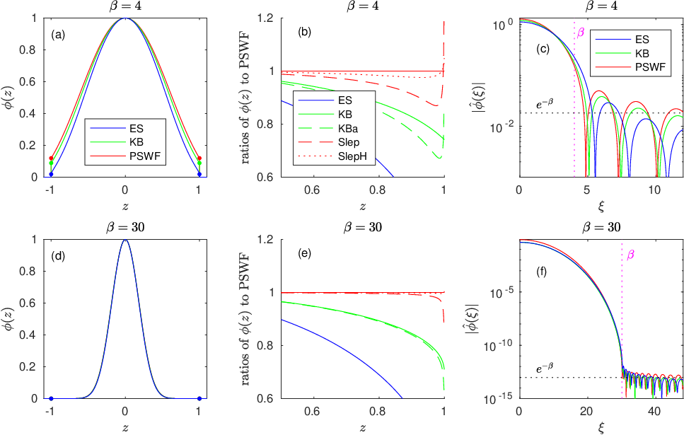
The main goal of this paper is to prove the following aliasing error convergence theorem applying to (7), which places this simple kernel (and hence algorithms which use it [5, 34]) on a rigorous footing. The rate will depend on the fixed upsampling factor $\sigma>1$. We also assume, as is usual with KB [12], a kernel parameter $\beta$ proportional to $w$. Specifically,

where $\gamma$ is a “safety factor”. At $\gamma=1$, the cutoff (see Fig. 1(c,f)) in $\hat{\psi}_{{\mbox{\tiny ES}},\beta}$ would coincide with the lowest aliased frequency $k=n-N/2$, so in practice one sets $\gamma<1$ (see Remark 3). Our main result concerns the constant $\varepsilon_{\infty}$ in the standard $\ell^{1}$-$\ell^{\infty}$ output error bounds

where we use vector notation ${\mathbf{c}}:=\{c_{j}\}_{j=1}^{M}$ and ${\mathbf{f}}:=\{f_{k}\}_{k=-N/2}^{N/2-1}$.

The rest of this paper breaks its proof into three stages: Section 2 reviews the standard bound for $\varepsilon_{\infty}$ involving a phased sum over the Fourier transform $\hat{\psi}$ of a general scaled kernel. Section 3 uses contour deformation and steepest descent to derive $\beta\to\infty$ asymptotics for $\hat{\phi}_{{\mbox{\tiny ES}},\beta}$, both below and above cutoff, then proves two technical lemmas on the decay of $\hat{\phi}_{{\mbox{\tiny ES}},\beta}$. Section 4 brings in two lemmas to handle phased sinc sums, then combines all of these ingredients to complete the proof.

We conclude the paper in Section 5 by drawing new connections—apparent in Fig. 1(b,e)—between the ES, KB, and PSWF kernels, and discussing their shared optimal rate.

Here we recall a known rigorous estimate on the error of the 1D type 1 and 2 algorithms given in the introduction, performed in exact arithmetic. We start with the Poisson summation formula with an extra phase $e^{i\theta}$: for any $\psi\in L^{1}(\mathbb{R})$ of bounded variation with Fourier transform $\hat{\psi}$, and any lattice spacing $h>0$,

The standard proof is that multiplication by $e^{-ix\theta/h}$ makes the left-hand side a periodic function of $x$, hence its Fourier series coefficients are given by the Euler–Fourier formula. At any points $x$ where the left-hand side is discontinuous, one must replace $\psi(x-lh)$ by $[\psi(x^{+}-lh)+\psi(x^{-}-lh)]/2$ [2, §11.22].

We now derive the aliasing error for a general scaled kernel $\psi(x)$. For the type 1 NUFFT, setting $h=2\pi/n$, inserting (3) into (4), and subtracting from the true answer (1) gives the error

Now writing the general ordinate as $x$, and applying Poisson summation (13) with $\theta=hk$,

The choice (5) for $p_{k}$ thus exactly kills the $m=0$ term, giving the well known aliasing error formula [37] [14, (4.1)] [12, Sec. V.B],

Thus, since $|k|\leq N/2$, error is controlled by a phased sum over the tails of $\hat{\psi}$ at frequencies of magnitude at least $n-N/2$. Since type 2 is the adjoint of type 1 (or by similar manipulations to the above), its error is

To summarize, let $E$ be the “error matrix” with elements $E_{kj}=g_{k}(x_{j})$ given explicitly by (15) and $E^{\ast}$ be its Hermitian adjoint, then the output aliasing error vectors are

From this the bounds (9) follow immediately if we define $\varepsilon_{\infty}$ by a simple uniform bound on all matrix elements,

Since the dynamic range over the output band, $\hat{\psi}(0)/\hat{\psi}(N/2)$, is not large [5, Remark 3], any lack of tightness in the second inequality in (18) is small.

Here we derive asymptotics in the width parameter $\beta\to\infty$ of the Fourier transform of (7). From now on we abbreviate the kernel by $\phi(z)$, thus its Fourier transform by $\hat{\phi}(\xi)$. We introduce the scaled frequency

The cutoff $|\xi|=\beta$ (vertical line in Fig. 1(c,f)) is therefore at $|\rho|=1$. The following shows that, up to weak algebraic prefactors: (a) below cutoff $\hat{\phi}$ has a similar form to $\phi$ itself, and that (b) above cutoff $\hat{\phi}$ is oscillatory but uniformly exponentially small, with the same exponential rate $e^{-\beta}$ as occurs for the KB and PSWF kernels (see Sec. 5).

Because of the above remark, in order to get a rigorous error estimate we will also need the following, which bounds the $\beta$-dependence of the deviation (denoted by $\hat{D}$) from the sinc function (25), uniformly in $\beta$ and for sufficiently high frequencies $\xi$. To avoid ambiguities involving asymptotics with two parameters (here $\beta$ and $\xi$), for the rest of the section we avoid “big-$O$” notation.

The above lemma excludes $|\xi|<\beta^{4}$, thus omts a growing (in $\beta$) number of terms in the sum (18), so, for the reason given in Remark 9, one cannot use the saddle asymptotic (21) to cover these terms. This motivates the following intermediate estimate which allows smaller frequencies, has explicit $\xi$ and $\beta$ dependence, but (because of its second term) fails to be summable in $\xi$.

Firstly, to handle Fourier tails due to (exponentially small) discontinuities at the edge of the support of $\phi$, we need the following technical lemmas. The first lemma bounds a conditionally convergent sinc sum, but needs the second lemma which uniformly bounds the difference between an exponential sum and a sinc function. Recall the definition $\sinc x:=(\sin x)/x$ for $x\neq 0$, or 1 otherwise.

References

- [1] F. Andersson, R. Moses, and F. Natterer. Fast Fourier methods for synthetic aperture radar imaging. IEEE Trans. Aerospace Elec. Sys., 48(1):215–229, 2012.
- [2] T. M. Apostol. Mathematical Analysis. Addison-Wesley, Reading, MA, 1974.
- [3] P. Arras, M. Reinecke, and R. Westermann. Efficient wide-field radio interferometry response, 2020. in preparation.
- [4] A. H. Barnett. How exponentially ill-conditioned are contiguous submatrices of the Fourier matrix?, 2020. arXiv:2004.09643. Submitted, SIAM Rev.
- [5] A. H. Barnett, J. F. Magland, and L. af Klinteberg. A parallel non-uniform fast Fourier transform library based on an “exponential of semicircle” kernel. SIAM J. Sci. Comput., 41(5):C479–C504, 2019.
- [6] G. Beylkin. On the fast Fourier transform of functions with singularities. Appl. Comput. Harmonic Anal., 2:363–383, 1995.
- [7] A. Böttcher and D. Potts. Probability against condition number and sampling of multivariate trigonometric random polynomials. Electron. Trans. Numer. Anal., 26:178–189, 2007.
- [8] T. M. Dunster. Uniform asymptotic expansions for prolate spheroidal functions with large parameters. SIAM J. Math. Anal., 17(6):1495–1524, 1986.
- [9] T. M. Dunster. Asymptotics of prolate spheroidal wave functions. J. Class. Anal., 11(1):1–21, 2017.
- [10] A. Dutt and V. Rokhlin. Fast Fourier transforms for nonequispaced data. SIAM J. Sci. Comput., 14:1369–1393, 1993.
- [11] J. Fessler. Michigan image reconstruction toolbox, 2016. Available at https://web.eecs.umich.edu/fessler/irt/fessler.tgz.
- [12] J. Fessler and B. Sutton. Nonuniform fast Fourier transforms using min-max interpolation. IEEE Trans. Signal Proc., 51(2):560–574, 2003.
- [13] K. Fourmont. Schnelle Fourier-Transformation bei nichtäquidistanten Gittern und tomographische Anwendungen. PhD thesis, Univ. Münster, 1999.
- [14] K. Fourmont. Non-equispaced fast Fourier transforms with applications to tomography. J. Fourier Anal. Appl., 9(5):431–450, 2003.
- [15] W. H. J. Fuchs. On the eigenvalues of an integral equation arising in the theory of band-limted signals. J. Math. Anal. Appl., 9:317–330, 1964.
- [16] Z. Gimbutas and S. Veerapaneni. A fast algorithm for spherical grid rotations and its application to singular quadrature. SIAM J. Sci. Comput., 5(6):A2738–A2751, 2013.
- [17] A. Goldstein and J. Abbate. Oral history: James Kaiser. http://ethw.org/Oral-History:James_Kaiser, 1997. online; accessed 2017-04-15.
- [18] L. Greengard and J.-Y. Lee. Accelerating the nonuniform fast Fourier transform. SIAM Review, 46(3):443–454, 2004.
- [19] J. I. Jackson, C. H. Meyer, D. G. Nishimura, and A. Macovski. Selection of a convolution function for Fourier inversion using gridding. IEEE Trans. Medical Imaging, 10(3):473–478, 1991.
- [20] M. Jacob. Optimized least-square nonuniform fast Fourier transform. IEEE Trans. Signal Process., 57(6):2165–2177, 2009.
- [21] J. Kaiser. Digital filters. In J. Kaiser and F. Kuo, editors, System analysis by digital computer, chapter 7, pages 218–285. Wiley, 1966.
- [22] J. Keiner, S. Kunis, and D. Potts. Using NFFT 3 — a software library for various nonequispaced fast Fourier transforms. ACM Trans. Math. Software, 36(4), 2009.
- [23] J.-M. Lin. Python non-uniform fast Fourier transform (PyNUFFT): An accelerated non-Cartesian MRI package on a heterogeneous platform (CPU/GPU). J. Imaging, 4(3):51, 2018.
- [24] J. Meixner and F. Schäfke. Mathieusche Funktionen und Sphäroidfunktionen. Springer, Berlin, 1954.
- [25] F. Nestler. Automated parameter tuning based on RMS errors for nonequispaced FFTs. Adv. Comput. Math., 42:889–919, 2016.
- [26] F. Nestler, M. Pippig, and D. Potts. Fast Ewald summation based on NFFT with mixed periodicity. J. Comput. Phys., 285:280–315, 2015.
- [27] F. Oberhettinger. Tables of Fourier transforms and Fourier transforms of distributions. Springer-Verlag, 1990.
- [28] K. Ogilvie. Rigorous asymptotics for the Lamé, Mathieu and spheroidal wave equations with a large parameter. PhD thesis, University of Edinburgh, 2016.
- [29] F. W. J. Olver. Asymptotics and special functions. Academic Press, New York, 1974.
- [30] F. W. J. Olver, D. W. Lozier, R. F. Boisvert, and C. W. Clark, editors. NIST Handbook of Mathematical Functions. Cambridge University Press, 2010. http://dlmf.nist.gov.
- [31] A. V. Oppenheim and R. W. Schafer. Discrete-time signal processing. Pearson Higher Education, Inc., 3rd edition, 2010.
- [32] A. Osipov, V. Rokhlin, and H. Xiao. Prolate Spheroidal Wave Functions of Order Zero: Mathematical Tools for Bandlimited Approximation, volume 187 of Applied Mathematical Sciences. Springer, US, 2013.
- [33] D. Potts and M. Tasche. Error estimates for nonequispaced fast Fourier transforms, 2020. arxiv:1912.09746v2.
- [34] D. S. Shamshirgar and A.-K. Tornberg. Fast Ewald summation for electrostatic potentials with arbitrary periodicity, 2017. arxiv:1712.04732.
- [35] D. Slepian. Some asymptotic expansions for prolate spheroidal wave functions. Journal of Mathematics and Physics, 44(1-4):99–140, 1965.
- [36] D. Slepian and H. O. Pollak. Prolate spheroidal wave functions, Fourier analysis and uncertainty, I. Bell Syst. Tech. J., 40:43–64, 1961.
- [37] G. Steidl. A note on fast Fourier transforms for nonequispaced grids. Adv. Comput. Math., 9:337–352, 1998.
- [38] M. Uecker and M. Lustig. BART toolbox for computational magnetic resonance imaging, 2016. DOI: 10.5281/zenodo.592960. Available at https://mrirecon.github.io/bart/.
- [39] K. Zhang and J. U. Kang. Graphics processing unit accelerated non-uniform fast Fourier transform for ultrahigh-speed, real-time Fourier-domain OCT. Opt. Express, 18(22):23472–87, 2010.