跳到论文正文
W Papers独立论文阅读器 arXiv:2001.09396 论文正文 计算阅读时间 · 0%
引用这篇论文根据当前论文元数据生成,正式投稿前建议核对。


License: arXiv.org perpetual non-exclusive license
arXiv:2001.09396v1 [cs.LG] 26 Jan 2020

Inference in Multi-Layer Networks with Matrix-Valued Unknowns

Parthe Pandit,1 Mojtaba Sahraee-Ardakan,1 Sundeep Rangan,2 Philip Schniter,3 and Alsyon K. Fletcher1 Affiliation: 1Dept. Statistics and ECE, University of California, Los Angeles Affiliation: 2Dept. ECE, New York University, Brooklyn, NY Affiliation: 3Dept. ECE, The Ohio State University, Columbus, Ohio
Abstract

We consider the problem of inferring the input and hidden variables of a stochastic multi-layer neural network from an observation of the output. The hidden variables in each layer are represented as matrices. This problem applies to signal recovery via deep generative prior models, multi-task and mixed regression, and learning certain classes of two-layer neural networks. A unified approximation algorithm for both MAP and MMSE inference is proposed by extending a recently-developed Multi-Layer Vector Approximate Message Passing (ML-VAMP) algorithm to handle matrix-valued unknowns. It is shown that the performance of the proposed Multi-Layer Matrix VAMP (ML-Mat-VAMP) algorithm can be exactly predicted in a certain random large-system limit, where the dimensions N×dN\times d of the unknown quantities grow as N→∞N\rightarrow\infty with dd fixed. In the two-layer neural-network learning problem, this scaling corresponds to the case where the number of input features and training samples grow to infinity but the number of hidden nodes stays fixed. The analysis enables a precise prediction of the parameter and test error of the learning.

I Introduction

𝐖1,𝐛1\mathbf{W}_{1},\mathbf{b}_{1}ϕ2​(⋅){\bm{\phi}}_{2}(\cdot)𝐖3,𝐛3\mathbf{W}_{3},\mathbf{b}_{3}ϕ4​(⋅){\bm{\phi}}_{4}(\cdot)𝐙00\mathbf{Z}^{0}_{0}𝐙10\mathbf{Z}^{0}_{1}𝐙20\mathbf{Z}^{0}_{2}𝐙30\mathbf{Z}^{0}_{3}𝐘\mathbf{Y}𝚵1{\bm{\Xi}}_{1}𝚵2{\bm{\Xi}}_{2}𝚵3{\bm{\Xi}}_{3}𝚵4{\bm{\Xi}}_{4}𝐆0+​(⋅)\mathbf{G}^{+}_{0}(\cdot)𝐆1±​(⋅)\mathbf{G}^{\pm}_{1}(\cdot)𝐆2±​(⋅)\mathbf{G}^{\pm}_{2}(\cdot)𝐆3±​(⋅)\mathbf{G}^{\pm}_{3}(\cdot)𝐆4−​(⋅)\mathbf{G}^{-}_{4}(\cdot)𝐘\mathbf{Y}𝐙^k​0+\widehat{\mathbf{Z}}^{+}_{k0}𝐑k​0+\mathbf{R}^{+}_{k0}𝐙^k​0−\widehat{\mathbf{Z}}^{-}_{k0}𝐑k​0−~\mathbf{R}^{-}_{k0}𝐙^k​1+\widehat{\mathbf{Z}}^{+}_{k1}𝐑k​1+\mathbf{R}^{+}_{k1}𝐙^k​1−\widehat{\mathbf{Z}}^{-}_{k1}𝐑k​1−~\mathbf{R}^{-}_{k1}𝐙^k​2+\widehat{\mathbf{Z}}^{+}_{k2}𝐑k​2+\mathbf{R}^{+}_{k2}𝐙^k​2−\widehat{\mathbf{Z}}^{-}_{k2}𝐑k​2−~\mathbf{R}^{-}_{k2}𝐙^k​3+\widehat{\mathbf{Z}}^{+}_{k3}𝐑k​3+\mathbf{R}^{+}_{k3}𝐙^k​3−\widehat{\mathbf{Z}}^{-}_{k3}𝐑k​3−~\mathbf{R}^{-}_{k3}
Fig. 1: (TOP) The signal flow graph for true values of matrix variables {𝐙ℓ0}ℓ=03\{\mathbf{Z}_{\ell}^{0}\}_{\ell=0}^{3}, given in eqn. (1) where 𝐙ℓ0∈ℝnℓ×d.\mathbf{Z}_{\ell}^{0}\in\mathbb{R}^{n_{\ell}\times d}. (BOTTOM) Signal flow graph of the ML-MVAMP procedure in Algo. 1. The variables with superscript + and - are updated in the forward and backward pass respectively. ML-MVAMP (Algorithm 1) solves (3) by solving a sequence of simpler estimation problems over consecutive pairs (𝐙ℓ,𝐙ℓ−1)(\mathbf{Z}_{\ell},\mathbf{Z}_{\ell-1}).

Consider an LL-layer stochastic neural network given by

𝐙ℓ0\displaystyle\mathbf{Z}^{0}_{\ell} =𝐖ℓ​𝐙ℓ−10+𝐁ℓ+𝚵ℓ0,\displaystyle=\mathbf{W}_{\ell}\mathbf{Z}^{0}_{\ell\!-\!1}+\mathbf{B}_{\ell}+{\bm{\Xi}}_{\ell}^{0},\quad ℓ\displaystyle\ell =1,3,…,L−1,\displaystyle=1,3,\ldots,L\!-\!1, (1a)
𝐙ℓ0\displaystyle\mathbf{Z}^{0}_{\ell} =ϕℓ​(𝐙ℓ−10,𝚵ℓ0),\displaystyle={\bm{\phi}}_{\ell}(\mathbf{Z}^{0}_{\ell\!-\!1},{\bm{\Xi}}_{\ell}^{0}),\quad ℓ\displaystyle\ell =2,4,…,L,\displaystyle=2,4,\ldots,L, (1b)

where, for ℓ=0,1,…,L\ell=0,1,\ldots,L, we have true activations 𝐙ℓ0∈ℝnℓ×d\mathbf{Z}_{\ell}^{0}\in\mathbb{R}^{n_{\ell}\times d}, weights 𝐖ℓ∈ℝnℓ×nℓ−1\mathbf{W}_{\ell}\in\mathbb{R}^{n_{\ell}\times n_{\ell-1}}, biases 𝐁ℓ∈ℝnℓ×d\mathbf{B}_{\ell}\in\mathbb{R}^{n_{\ell}\times d}, and true noise realizations 𝚵ℓ0{\bm{\Xi}}_{\ell}^{0}. The activation functions ϕℓ{\bm{\phi}}_{\ell} are known, non-linear functions acting row-wise on their inputs. See Fig. 1 (TOP). We use the superscript 0 in 𝐙ℓ0\mathbf{Z}_{\ell}^{0} to indicate the true values of the variables, in contrast to estimated values discussed later. We model the true values 𝐙00\mathbf{Z}^{0}_{0} as a realization of random 𝐙0\mathbf{Z}_{0}, where the rows 𝐳0,i:T\mathbf{z}_{0,i:}^{\text{\sf T}} of 𝐙0\mathbf{Z}_{0} are i.i.d. with distribution p0p_{0}:

p(𝐙0)=∏i=1n0p0(𝐳0,i:).p(\mathbf{Z}_{0})=\prod_{i=1}^{n_{0}}p_{0}(\mathbf{z}_{0,i:}). (2)

Similarly, we also assume that 𝚵ℓ0{\bm{\Xi}}_{\ell}^{0} are realizations of random 𝚵ℓ{\bm{\Xi}}_{\ell} with i.i.d. rows 𝝃ℓ,i:T{\bm{\xi}}_{\ell,i:}^{\text{\sf T}}. For odd ℓ\ell, the rows 𝝃ℓ,i:{\bm{\xi}}_{\ell,i:} are zero-mean multivariate Gaussian with covariance 𝐍ℓ−1∈ℝd×d\mathbf{N}_{\ell}^{-1}\in\mathbb{R}^{d\times d}, whereas for even ℓ\ell, the rows 𝝃ℓ,i:{\bm{\xi}}_{\ell,i:} can be arbitrarily distributed but i.i.d.

Denoting by 𝐘:=𝐙L0∈ℝnL×d\mathbf{Y}:=\mathbf{Z}_{L}^{0}\in\mathbb{R}^{n_{L}\times d} the output of the network, we consider the following matrix inference problem:

Estimate​𝐙:={𝐙ℓ}ℓ=0L−1\displaystyle\rm{\displaystyle Estimate\ }\mathbf{Z}:=\{\mathbf{Z}_{\ell}\}_{\ell=0}^{L-1} (3)
given​𝐘:=𝐙L0​and​{𝐖2​k−1,𝐁2​k−1,ϕ2​k}k=1L/2.\displaystyle\rm{\displaystyle given\ }\mathbf{Y}:=\mathbf{Z}^{0}_{L}{\rm\ and\ }\{\mathbf{W}_{2k-1},\mathbf{B}_{2k-1},{\bm{\phi}}_{2k}\}_{k=1}^{L/2}.

This inference problem arises in reconstruction with deep generative priors [1, 2]: A deep neural network is trained as a generative model for some complex data, such as an image. The generative model could be a variational auto-encoder (VAE) [3, 4], generative adversarial network (GAN) [5, 6], or deep image prior (DIP) [7, 8]. The generative model is driven by some noise-like innovations signal 𝐙00\mathbf{Z}^{0}_{0}. Subsequent layers are then appended to model a lossy measurement process such as blurring, occlusion, or noise, resulting in a corrupted output 𝐘\mathbf{Y}. With the addition of the measurement layer(s), the original image or data manifests as one of the hidden variables in the network. The problem of estimating the original image from the output 𝐘\mathbf{Y} is then equivalent to the inference problem (3) of estimating the values of a hidden layer in a multi-layer network from its output. Note that, in this application, the problem is not the “learning problem” for the network, since the weights and biases of the network are assumed known (i.e., trained).

In many applications, the network (1) has no noise 𝚵ℓ{\bm{\Xi}}_{\ell} for all layers except the final one, ℓ=L\ell=L. In this case, the 𝐙L−10=𝐠⁡(𝐙00)\mathbf{Z}^{0}_{L-1}=\mathbf{g}(\mathbf{Z}_{0}^{0}) for some deterministic function 𝐠⁡(⋅)\mathbf{g}(\cdot) representing the action of the first L−1L-1 layers. Inference can then be conducted via a minimization of the form,

𝐙^0:=arg​min𝐙0⁡HL​(𝐘,𝐙L−1)+H0​(𝐙0),\widehat{\mathbf{Z}}_{0}:=\argmin_{\mathbf{Z}_{0}}H_{L}(\mathbf{Y},\mathbf{Z}_{L-1})+H_{0}(\mathbf{Z}_{0}), (4)

where 𝐙L−1=𝐠⁡(𝐙0)\mathbf{Z}_{L-1}=\mathbf{g}(\mathbf{Z}_{0}) is the network output, the term HL​(𝐘,𝐙L−1)H_{L}(\mathbf{Y},\mathbf{Z}_{L-1}) penalizes the prediction error and H0​(𝐙0)H_{0}(\mathbf{Z}_{0}) is an (optional) regularizer on the network input. For maximum a priori (MAP) estimation one takes,

HL​(𝐘,𝐙L−1)\displaystyle H_{L}(\mathbf{Y},\mathbf{Z}_{L-1}) =−log⁡p⁡(𝐘|𝐙L−1),\displaystyle=-\log p(\mathbf{Y}|\mathbf{Z}_{L-1}), (5a)
H0​(𝐙0)\displaystyle H_{0}(\mathbf{Z}_{0}) =−log⁡p⁡(𝐙0),\displaystyle=-\log p(\mathbf{Z}_{0}), (5b)

where the output probability p⁡(𝐘|𝐙L−1)p(\mathbf{Y}|\mathbf{Z}_{L-1}) is defined from the last layer of model (1b): 𝐘=𝐙L=ϕL​(𝐙L−1,𝚵L)\mathbf{Y}=\mathbf{Z}_{L}={\bm{\phi}}_{L}(\mathbf{Z}_{L-1},{\bm{\Xi}}_{L}). The minimization (4) can then be solved using a gradient-based method. Encouraging results in image reconstruction have been demonstrated in [1, 2, 9, 10, 11, 12, 13]. Markov-chain Monte Carlo (MCMC) algorithms and Langevin diffusion [14, 15] could also be employed for more complex inference tasks. However, rigorous analysis of these methods is difficult due to the non-convex nature of the optimization problem. To address this issue, recent works [16, 17, 18] have extended Approximate Message Passing (AMP) methods to provide inference algorithms for the multi-layer networks. AMP was originally developed in [19, 20, 21] for compressed sensing. Similar to other AMP-type results, the performance of multi-layer AMP-based inference can be precisely characterized in certain high-dimensional random instances. In addition, the mean-squared error for inference of the algorithms match predictions for the Bayes-optimal inference predicted by various techniques from statistical physics [22, 23, 24]. Thus, AMP-based multi-layer inference provides a computationally tractable estimation framework with precise performance guarantees and testable conditions for optimality in certain high-dimensional random settings.

Prior multi-layer AMP works [25, 16, 17, 18] have considered the case of vector-valued quantities with d=1d=1. The main contribution of this paper is to consider the matrix-valued case when d>1d>1. As we will see in Section II, the matrix-valued case applies to multi-task and mixed regression problems, sketched clustering, as well as learning certain classes of two layer networks.

To handle the case when d>1d>1, we extend the Multi-Layer Vector Approximate Message Passing (ML-VAMP) algorithm of [17, 18] to the matrix case. The ML-VAMP method is based on VAMP method of [26], which is closely related to expectation propagation (EP) [27, 28], expectation-consistent approximate inference (EC) [29, 30], S-AMP [31], and orthogonal AMP [32]. We will use “ML-Mat-VAMP” when referring to the matrix extension of ML-VAMP.

Similar to the case of ML-VAMP, we analyze ML-Mat-VAMP in a large system limit, where nℓ→∞n_{\ell}\rightarrow\infty and dd is fixed, under rotationally invariant random weight matrices 𝐖ℓ\mathbf{W}_{\ell}. In this large system limit, we prove that the mean-squared error (MSE) of the estimates of ML-Mat-VAMP can be exactly predicted by a deterministic set of equations called the state evolution (SE). In the case of ML-VAMP, the SE equations involve scalar quantities and 2×22\times 2 matrices. For ML-Mat-VAMP, the SE equations involve d×dd\times d and 2​d×2​d2d\times 2d matrices. For learning problems, we will see that the SE equations enables predictions of the parameter error as well as test error.

Notation

: Boldface uppercase letters 𝐗\mathbf{X} denote matrices. 𝐗n:\mathbf{X}_{n:} refers to the nthn^{\rm th} row of 𝐗\mathbf{X}. Random vectors are row-vectors. For a function f:ℝ1×m→ℝ1×n,f:\mathbb{R}^{1\times m}\rightarrow\mathbb{R}^{1\times n}, its row-wise extension is represented by 𝐟:ℝN×m→ℝN×n\mathbf{f}:\mathbb{R}^{N\times m}\rightarrow\mathbb{R}^{N\times n}, i.e., [𝐟(𝐗)]n:=f(𝐗n:)[\mathbf{f}(\mathbf{X})]_{n:}=f(\mathbf{X}_{n:}). We denote the Jacobian matrix of ff by ∂f∂𝒙​(𝒙,𝒚)∈ℝm×n\tfrac{\partial f}{\partial\bm{x}}(\bm{x},\bm{y})\in\mathbb{R}^{m\times n}, so that [∂f∂𝒙​(𝒙,𝒚)]i​j=∂fi∂𝒙j​(𝒙,𝒚)[\tfrac{\partial f}{\partial\bm{x}}(\bm{x},\bm{y})]_{ij}=\tfrac{\partial f_{i}}{\partial\bm{x}_{j}}(\bm{x},\bm{y}). For its row-wise extension 𝐟\mathbf{f}, we denote by ⟨∂𝐟∂𝐗​(𝐗,𝐘)⟩\langle{\tfrac{\partial\mathbf{f}}{\partial\mathbf{X}}(\mathbf{X},\mathbf{Y})}\rangle the average Jacobian, i.e., 1N∑n=1N∂f∂𝐗n:(𝐗n:,𝐘n:)\tfrac{1}{N}\sum_{n=1}^{N}\tfrac{\partial f}{\partial\mathbf{X}_{n:}}(\mathbf{X}_{n:},\mathbf{Y}_{n:})

II Example Applications

II-A Multi-task and Mixed Regression Problems

A simple application of the matrix-valued multi-layer inference problem (3) is for multi-task regression [33]. Consider a linear model of the form,

𝐘=𝐗𝐅+𝚵,\mathbf{Y}=\mathbf{X}\mathbf{F}+{\bm{\Xi}}, (6)

where 𝐘∈ℝN×d\mathbf{Y}\in{\mathbb{R}}^{N\times d} is a matrix of measured responses, 𝐗∈ℝN×p\mathbf{X}\in{\mathbb{R}}^{N\times p} is a known matrix, 𝐅∈ℝp×d\mathbf{F}\in{\mathbb{R}}^{p\times d} are a set regression coefficients to be estimated, and 𝚵{\bm{\Xi}} is additive noise. The problem can be considered as dd separate linear regression problems – one for each column. However, in some applications, these design “tasks” are related in such a way that it benefits to jointly estimate the predictors. To do this, it is common to solve an optimization problem of the form

argmin𝐅{∑j=1d∑i=1NL(yi​j,[𝐗𝐅]i​j)+λ∑k=1pρ(𝐅k:)},\arg\min_{\mathbf{F}}\Bigg\{\sum_{j=1}^{d}\sum_{i=1}^{N}L(y_{ij},[\mathbf{X}\mathbf{F}]_{ij})+\lambda\sum_{k=1}^{p}\rho(\mathbf{F}_{k:})\Bigg\}, (7)

where L⁡(⋅)L(\cdot) is a loss function, and ρ⁡(⋅)\rho(\cdot) is a regularizer that acts on the rows of 𝐅k:\mathbf{F}_{k:} of 𝐅\mathbf{F} to couple the prediction coefficients across tasks. For example, the multi-task LASSO [33] uses loss L⁡(y,z)=(y−z)2L(y,z)=(y-z)^{2} and regularization ρ(𝐅k:)=∥𝐅k:∥2\rho(\mathbf{F}_{k:})=\|\mathbf{F}_{k:}\|_{2} to enforce row-sparsity in 𝐅\mathbf{F}. In the compressive-sensing context, multi-task regression is known as the “multiple measurement vector” (MMV) problem, with applications in MEG reconstruction [34], DoA estimation [35], and parallel MRI [36]. An AMP approach to the MMV problem was developed in [37]. The multi-task model (6) can be immediately written as a multi-layer network (1) by setting:

𝐙0\displaystyle\mathbf{Z}_{0} :=𝐅,𝐖0:=𝐗,\displaystyle:=\mathbf{F},\quad\mathbf{W}_{0}:=\mathbf{X},
𝐙1\displaystyle\mathbf{Z}_{1} :=𝐖0​𝐙0=𝐗𝐅,𝐘=𝐙2:=𝐙1+𝚵.\displaystyle:=\mathbf{W}_{0}\mathbf{Z}_{0}=\mathbf{X}\mathbf{F},\quad\mathbf{Y}=\mathbf{Z}_{2}:=\mathbf{Z}_{1}+{\bm{\Xi}}.

Also, by appropriately setting the prior p⁡(𝐙0)p(\mathbf{Z}_{0}), the multi-layer matrix MAP inference (5) will match the multi-task optimization (7).

In (7), the regularization couples the columns of 𝐅\mathbf{F} but the loss term does not. In mixed regression problems, the loss couples the columns of 𝐅\mathbf{F}. For example, consider designing predictors 𝐅=[𝐟1,𝐟2]\mathbf{F}=[\mathbf{f}_{1},\mathbf{f}_{2}] for mixed linear regression [38], i.e.,

yi=qi​𝐱iT​𝐟1+(1−qi)​𝐱iT​𝐟2+vi,qi∈{0,1},y_{i}=q_{i}\mathbf{x}_{i}^{\text{\sf T}}\mathbf{f}_{1}+(1-q_{i})\mathbf{x}_{i}^{\text{\sf T}}\mathbf{f}_{2}+v_{i},~~q_{i}\in\{0,1\}, (8)

where i=1,…,Ni=1,\ldots,N and the iith response comes from one of two linear models, but which model is not known. This setting can be modeled by a different output mapping: As before, set 𝐙1=𝐗𝐅\mathbf{Z}_{1}=\mathbf{X}\mathbf{F} and let the noise in the output layer be 𝚵1=[𝐪,𝐯]{\bm{\Xi}}_{1}=[\mathbf{q},\mathbf{v}] which includes the additive noise viv_{i} in (8) and the random selection variable qiq_{i}. Then, we can write (8) via an appropriate function, 𝐲=ϕ1​(𝐙1,𝚵1)\mathbf{y}={\bm{\phi}}_{1}(\mathbf{Z}_{1},{\bm{\Xi}}_{1}).

II-B Sketched Clustering

A related problem arises in sketched clustering [39], where a massive dataset is nonlinearly compressed down to a short vector 𝐲∈ℝn\mathbf{y}\in\mathbb{R}^{n}, from which cluster centroids 𝐟k∈ℝp\mathbf{f}_{k}\in\mathbb{R}^{p}, for k=1,…,dk=1,\dots,d, are then extracted. This problem can be approached via the optimization [40]

min𝜶≥𝟎⁡min⁡∑i=1n𝐅⁡|yi−∑j=1dαj​e−1​𝐱iT​𝐟j|2,\min_{{\bm{\alpha}}\geq\mathbf{0}}\min_{\mathbf{F}}\sum_{i=1}^{n}\bigg|y_{i}-\sum_{j=1}^{d}\alpha_{j}e^{\sqrt{-1}\mathbf{x}_{i}^{\text{\sf T}}\mathbf{f}_{j}}\bigg|^{2}, (9)

where 𝐱i∈ℝp\mathbf{x}_{i}\in\mathbb{R}^{p} are known i.i.d. Gaussian vectors. An AMP approach to sketched clustering was developed in [41]. For known 𝜶{\bm{\alpha}}, the minimization corresponds to MAP estimation with the multi-layer matrix model with 𝐙0=𝐅\mathbf{Z}_{0}=\mathbf{F}, 𝐖1=𝐗\mathbf{W}_{1}=\mathbf{X} 𝐙1=𝐗𝐅\mathbf{Z}_{1}=\mathbf{X}\mathbf{F} and using the output mapping,

ϕ1(𝐙1,𝚵):=∑j=1dαje−1𝐙1,:j+𝚵,{\bm{\phi}}_{1}(\mathbf{Z}_{1},{\bm{\Xi}}):=\sum_{j=1}^{d}\alpha_{j}e^{\sqrt{-1}\mathbf{Z}_{1,:j}}+{\bm{\Xi}},

where the exponential is applied elementwise and 𝚵{\bm{\Xi}} is i.i.d. Gaussian. The mapping ϕ1\phi_{1} operates row-wise on 𝐙1\mathbf{Z}_{1} and 𝚵{\bm{\Xi}}.

II-C Learning the Input Layer of a Two-Layer Neural Network

The matrix inference problem (3) can also be applied to learning the input layer weights in a two-layer neural network (NN). Let 𝐗∈ℝN×Nin\mathbf{X}\in{\mathbb{R}}^{N\times N_{\rm in}} and 𝐘∈ℝN×Nout\mathbf{Y}\in{\mathbb{R}}^{N\times N_{\rm out}} be training data corresponding to NN data samples. Consider the two-layer NN model,

𝐘=σ⁡(𝐗​𝑭1)​𝑭2+𝚵,\mathbf{Y}=\sigma(\mathbf{X}\bm{F}_{1})\bm{F}_{2}+{\bm{\Xi}}, (10)

with weight matrices (𝑭1,𝑭2)(\bm{F}_{1},\bm{F}_{2}), componentwise activation function σ⁡(⋅)\sigma(\cdot), and noise 𝚵{\bm{\Xi}}. In (10), the bias terms are omitted for simplicity. We used the notation “𝑭ℓ\bm{F}_{\ell}” for the weights, instead of the standard notation “𝑾ℓ\bm{W}_{\ell},” to avoid confusion when (10) is mapped to the multi-layer inference network (3). Now, our critical assumption is that the weights in the second layer, 𝑭2\bm{F}_{2}, are known. The goal is to learn only the weights of the first layer, 𝑭1∈ℝNin×Nhid\bm{F}_{1}\in\mathbb{R}^{N_{\rm in}\times N_{\rm hid}}, from a dataset of NN samples (𝐗,𝐘)(\mathbf{X},\mathbf{Y}).

If the activation is ReLU, i.e., σ⁡(𝑯)=max⁡{𝑯,0}\sigma(\bm{H})=\max\{\bm{H},0\} and 𝐘\mathbf{Y} has a single column (i.e. scalar output per sample), and 𝑭2\bm{F}_{2} has all positive entries, we can w.l.o.g. treat the weights 𝑭2\bm{F}_{2} as fixed, since they can always be absorbed into the weights 𝑭1\bm{F}_{1}. In this case, 𝐲\mathbf{y} and 𝐅2\mathbf{F}_{2} are vectors and we can write the iith entry of 𝐲\mathbf{y} as

yi=∑j=1dF2​j​σ​([𝐗​𝑭1]i​j)+ξi=∑j=1dσ⁡([𝐗​𝑭1]i​j​F2​j)+ξiy_{i}=\sum_{j=1}^{d}F_{2j}\sigma([\mathbf{X}\bm{F}_{1}]_{ij})+\xi_{i}=\sum_{j=1}^{d}\sigma([\mathbf{X}\bm{F}_{1}]_{ij}F_{2j})+\xi_{i} (11)

Thus, we can assume w.l.o.g. that 𝐅2\mathbf{F}_{2} is all ones. The parameterization (11) is sometimes referred to as the committee machine [42]. The committee machine has been recently studied by AMP methods [43] and mean-field methods [44] as a way to understand the dynamics of learning.

To pose the two-layer learning problem as multi-layer inference, define

𝒁0:=𝑭1,𝑾1:=𝐗,𝒁1:=𝐗​𝑭1𝚵2:=𝚵,\bm{Z}_{0}:=\bm{F}_{1},\quad\bm{W}_{1}:=\mathbf{X},\quad\bm{Z}_{1}:=\mathbf{X}\bm{F}_{1}\quad{\bm{\Xi}}_{2}:={\bm{\Xi}},

then 𝒀=𝒁2\bm{Y}=\bm{Z}_{2}, where 𝒁2\bm{Z}_{2} is the output of a 2-layer inference network of the form in (1):

𝐘=𝒁2=ϕ2​(𝒁1,𝚵2):=σ⁡(𝒁1)​𝑭2+𝚵2.\mathbf{Y}=\bm{Z}_{2}={\bm{\phi}}_{2}(\bm{Z}_{1},{\bm{\Xi}}_{2}):=\sigma(\bm{Z}_{1})\bm{F}_{2}+{\bm{\Xi}}_{2}. (12)

Note that 𝑾1\bm{W}_{1} is known. Also, since we have assumed that 𝑭2\bm{F}_{2} is known, the function ϕ2{\bm{\phi}}_{2} is known. Finally, the function ϕ2{\bm{\phi}}_{2} is row-wise separable on both inputs. Thus, the problem of learning the input weights 𝑭1\bm{F}_{1} is equivalent to learning the input 𝒁0\bm{Z}_{0} of the network (12).

III Multi-layer Matrix VAMP

III-A MAP and MMSE inference

Observe that the equations (1) define a Markov chain over these signals and thus the posterior p⁡(𝐙|𝐙L)p(\mathbf{Z}|\mathbf{Z}_{L}) factorizes as

p⁡(𝐙|𝐙L)∝p⁡(𝐙0)​∏ℓ=1L−1p⁡(𝐙ℓ|𝐙ℓ−1)​p​(𝐘|𝐙L−1).p(\mathbf{Z}|\mathbf{Z}_{L})\propto p(\mathbf{Z}_{0})\prod_{\ell=1}^{L-1}p(\mathbf{Z}_{\ell}|\mathbf{Z}_{\ell-1})\,p(\mathbf{Y}|\mathbf{Z}_{L-1}). (13)

where the transition probabilities p⁡(𝐙ℓ|𝐙ℓ−1)p(\mathbf{Z}_{\ell}|\mathbf{Z}_{\ell-1}) are implicitly defined in equation (1) and depend on the statistics of noise terms 𝚵ℓ{\bm{\Xi}}_{\ell}. We consider both maximum a posteriori (MAP) and minimum mean squared error (MMSE) estimation for this posterior:

𝐙^𝗆𝖺𝗉\displaystyle\widehat{\mathbf{Z}}_{\sf{map}} =arg​max𝐙⁡p​(𝐙|𝐙L)\displaystyle=\argmax_{\mathbf{Z}}\ p(\mathbf{Z}|\mathbf{Z}_{L}) (14a)
𝐙^𝗆𝗆𝗌𝖾\displaystyle\widehat{\mathbf{Z}}_{\mathsf{mmse}} =𝔼⁡[𝐙|𝐙L]=∫𝐙​p​(𝐙|𝐙L)​⁡𝑑𝐙.\displaystyle=\mathbb{E}[\mathbf{Z}|\mathbf{Z}_{L}]=\int\mathbf{Z}\,p(\mathbf{Z}|\mathbf{Z}_{L})\mathop{}\!\mathrm{d}\mathbf{Z}. (14b)

III-B Algorithm Details

The ML-Mat-VAMP for approximately computing the MAP and MMSE estimates is similar to the ML-VAMP method in [17, 45]. The specific iterations of ML-Mat-VAMP algorithm are shown in Algorithm 1. The algorithm produces estimates by a sequence of forward and backward pass updates denoted by superscripts + and - respectively.

The estimates 𝐙^ℓ±\widehat{\mathbf{Z}}^{\pm}_{\ell} are constructed by solving sequential problems 𝐙={𝐙ℓ}ℓ=0ℓ−1\mathbf{Z}=\{\mathbf{Z}_{\ell}\}_{\ell=0}^{\ell-1} into a sequence of smaller problems each involving estimation of a single activation or preactivation 𝐙ℓ\mathbf{Z}_{\ell} via estimation functions {𝐆ℓ±​(⋅)}ℓ=1L−1\{\mathbf{G}_{\ell}^{\pm}(\cdot)\}_{\ell=1}^{L-1} which are selected depending on whether one is interested in MAP or MMSE estimation.

To describe the estimation functions, we use the notation that, for a positive definite matrix 𝚪{\bm{\Gamma}}, define the inner product ⟨𝐀,𝐁⟩Γ:=Tr⁡(𝐀T​𝐁​𝚪)\langle{\mathbf{A},\mathbf{B}}\rangle_{\Gamma}:=\mathrm{Tr}(\mathbf{A}^{\text{\sf T}}\mathbf{B}{\bm{\Gamma}}) and let ‖𝐀‖𝚪\left\|\mathbf{A}\right\|_{{\bm{\Gamma}}} denote the norm induced by this inner product. For ℓ=1,…,L−1\ell=1,\ldots,L-1 define the approximate belief functions

bℓ(𝐙ℓ,𝐙ℓ−1|𝐑ℓ−,𝐑ℓ−1+,𝚪ℓ−,𝚪ℓ−1+)∝p(𝐙ℓ|𝐙ℓ−1)\displaystyle b_{\ell}(\mathbf{Z}_{\ell},\mathbf{Z}_{\ell-1}|\mathbf{R}_{\ell}^{-},\mathbf{R}_{\ell-1}^{+},{\bm{\Gamma}}_{\ell}^{-},{\bm{\Gamma}}_{\ell-1}^{+})\propto p(\mathbf{Z}_{\ell}|\mathbf{Z}_{\ell-1}) (15)
×e−12​‖𝐙ℓ−𝐑ℓ−‖𝚪ℓ−2−12​‖𝐙ℓ−1−𝐑ℓ−1+‖𝚪ℓ−1+2.\displaystyle\times e^{-\frac{1}{2}\left\|\mathbf{Z}_{\ell}-\mathbf{R}_{\ell}^{-}\right\|_{{\bm{\Gamma}}_{\ell}^{-}}^{2}-\frac{1}{2}\left\|\mathbf{Z}_{\ell-1}-\mathbf{R}_{\ell-1}^{+}\right\|_{{\bm{\Gamma}}_{\ell-1}^{+}}^{2}}.

Define b0​(𝐙0|𝐑0−,𝚪0−)b_{0}(\mathbf{Z}_{0}|\mathbf{R}_{0}^{-},{\bm{\Gamma}}_{0}^{-}) and bL​(𝐙L−1|𝐑L−1+,𝚪L−1+)b_{L}(\mathbf{Z}_{L-1}|\mathbf{R}_{L-1}^{+},{\bm{\Gamma}}_{L-1}^{+}) similarly.

Algorithm 1 Multilayer Matrix VAMP (ML-Mat-VAMP)
0:  Estimators 𝐆0+\mathbf{G}_{0}^{+}, 𝐆L−\mathbf{G}_{L}^{-}, {𝐆ℓ±}ℓ=1L−1\{\mathbf{G}_{\ell}^{\pm}\}_{\ell=1}^{L-1}.
1:  Set 𝐑0​ℓ−=𝟎\mathbf{R}^{-}_{0\ell}=\mathbf{0} and initialize {𝚪0​ℓ−}ℓ=0L−1\{{\bm{\Gamma}}_{0\ell}^{-}\}_{\ell=0}^{L-1}.
2:  for k=0,1,…,Nit−1k=0,1,\dots,N_{\rm it}-1 do
3:   // Forward Pass
4:   𝐙^k​0+=𝐆0+​(𝐑k​0−,𝚪k​0−)\widehat{\mathbf{Z}}^{+}_{k0}=\mathbf{G}_{0}^{+}(\mathbf{R}^{-}_{k0},{\bm{\Gamma}}_{k0}^{-})
5:   𝚲k​0+=⟨∂𝐆0+∂𝐑k,0−​(𝐑k​0−,𝚪k​0−)⟩−1​𝚪k,0−,\mathbf{\Lambda}^{+}_{k0}={\left<\tfrac{\partial\mathbf{G}_{0}^{+}}{\partial\mathbf{R}^{-}_{k,0}}(\mathbf{R}^{-}_{k0},{\bm{\Gamma}}_{k0}^{-})\right>}^{-1}{\bm{\Gamma}}_{k,0}^{-},
6:   𝚪k,0+=𝚲k,0+−𝚪k,0−{\bm{\Gamma}}_{k,0}^{+}=\mathbf{\Lambda}_{k,0}^{+}-{\bm{\Gamma}}_{k,0}^{-}
7:   𝐑k,0+=(𝐙^k,0+​𝚲k,0+−𝐑k,0−​𝚪k,0−)​(𝚪k,0+)−1\mathbf{R}^{+}_{k,0}=(\widehat{\mathbf{Z}}^{+}_{k,0}\mathbf{\Lambda}_{k,0}^{+}-\mathbf{R}^{-}_{k,0}{\bm{\Gamma}}^{-}_{k,0})({\bm{\Gamma}}_{k,0}^{+})^{-1}
8:   for ℓ=1,…,L−1\ell=1,\ldots,L\!-\!1 do
9:    𝐙^k​ℓ+=𝐆ℓ+​(𝐑k​ℓ−,𝐑k,ℓ−1+,𝚪k​ℓ−,𝚪k,ℓ−1+)\widehat{\mathbf{Z}}^{+}_{k\ell}=\mathbf{G}_{\ell}^{+}(\mathbf{R}^{-}_{k\ell},\mathbf{R}^{+}_{k,\ell\!-\!1},{\bm{\Gamma}}_{k\ell}^{-},{\bm{\Gamma}}^{+}_{k,\ell-1})
10:    𝚲k​ℓ+=⟨∂𝐆ℓ+∂𝐑ℓ−​(𝐑k​ℓ−,𝐑k,ℓ−1+,𝚪k​ℓ−,𝚪k,ℓ−1+)⟩−1​𝚪k,ℓ−,\mathbf{\Lambda}^{+}_{k\ell}={\left<\tfrac{\partial\mathbf{G}_{\ell}^{+}}{\partial\mathbf{R}^{-}_{\ell}}(\mathbf{R}^{-}_{k\ell},\mathbf{R}^{+}_{k,\ell\!-\!1},{\bm{\Gamma}}_{k\ell}^{-},{\bm{\Gamma}}^{+}_{k,\ell-1})\right>}^{-1}{\bm{\Gamma}}_{k,\ell}^{-},
11:    𝚪k,ℓ+=𝚲k,ℓ+−𝚪k,ℓ−{\bm{\Gamma}}_{k,\ell}^{+}=\mathbf{\Lambda}_{k,\ell}^{+}-{\bm{\Gamma}}_{k,\ell}^{-}
12:    𝐑k​ℓ+=(𝐙^k,ℓ+​𝚲k,ℓ+−𝐑k,ℓ−​𝚪k,ℓ−)​(𝚪k,ℓ+)−1\mathbf{R}^{+}_{k\ell}=(\widehat{\mathbf{Z}}^{+}_{k,\ell}\mathbf{\Lambda}_{k,\ell}^{+}-\mathbf{R}^{-}_{k,\ell}{\bm{\Gamma}}^{-}_{k,\ell})({\bm{\Gamma}}_{k,\ell}^{+})^{-1}
13:   end for
14:   
15:   // Backward Pass
16:   𝐙^k,L−1−=𝐆L−​(𝐑k,L−1+,𝚪k,L−1+)\widehat{\mathbf{Z}}^{-}_{k,L\!-\!1}=\mathbf{G}_{L}^{-}(\mathbf{R}^{+}_{k,L\!-\!1},{\bm{\Gamma}}_{k,L\!-\!1}^{+})
17:   𝚲k,L−1−=⟨∂𝐆L−∂𝐑k,L−1+​(𝐑k,L−1+,𝚪k,L−1+)⟩−1​𝚪k,L−1+,\mathbf{\Lambda}^{-}_{k,L\!-\!1}={\left<\tfrac{\partial\mathbf{G}_{L}^{-}}{\partial\mathbf{R}^{+}_{k,L\!-\!1}}(\mathbf{R}^{+}_{k,L\!-\!1},{\bm{\Gamma}}_{k,L\!-\!1}^{+})\right>}^{-1}{\bm{\Gamma}}_{k,L\!-\!1}^{+},
18:   𝚪k,L−1−=𝚲k,L−1−−𝚪k,L−1+{\bm{\Gamma}}_{k,L\!-\!1}^{-}=\mathbf{\Lambda}_{k,L\!-\!1}^{-}-{\bm{\Gamma}}_{k,L\!-\!1}^{+}
19:   𝐑k+1,L−1−=(𝐙^k,L−1−​𝚲k,L−1−−𝐑k,0+​𝚪k,0+)​(𝚪k,0−)−1\mathbf{R}^{-}_{k\!+\!1,L\!-\!1}=(\widehat{\mathbf{Z}}^{-}_{k,L\!-\!1}\mathbf{\Lambda}_{k,L\!-\!1}^{-}-\mathbf{R}^{+}_{k,0}{\bm{\Gamma}}^{+}_{k,0})({\bm{\Gamma}}_{k,0}^{-})^{-1}
20:   for ℓ=L−1,…,1\ell=L\!-\!1,\ldots,1 do
21:    𝐙^k+1,ℓ−1−=𝐆ℓ−​(𝐑k+1,ℓ−,𝐑k,ℓ−1+,𝚪k+1,ℓ−,𝚪k,ℓ−1+)\widehat{\mathbf{Z}}^{-}_{k+1,\ell-1}=\mathbf{G}_{\ell}^{-}(\mathbf{R}^{-}_{k+1,\ell},\mathbf{R}^{+}_{k,\ell-1},{\bm{\Gamma}}_{k+1,\ell}^{-},{\bm{\Gamma}}^{+}_{k,\ell-1})
22:    𝚲k+1,ℓ−1−=⟨∂𝐆ℓ−∂𝐑ℓ−1+​(⋯)⟩−1​𝚪k,ℓ−1+,\mathbf{\Lambda}^{-}_{k+1,\ell-1}={\left<\tfrac{\partial\mathbf{G}_{\ell}^{-}}{\partial\mathbf{R}^{+}_{\ell-1}}(\cdots)\right>}^{-1}{\bm{\Gamma}}_{k,\ell\!-\!1}^{+},
23:    𝚪k+1,ℓ−=𝚲k,ℓ−−𝚪k,ℓ+{\bm{\Gamma}}_{k+1,\ell}^{-}=\mathbf{\Lambda}_{k,\ell}^{-}-{\bm{\Gamma}}_{k,\ell}^{+}
24:    𝐑k+1,ℓ−1−=(𝐙^k,ℓ−​𝚲k,ℓ−−𝐑k,ℓ+​𝚪k,ℓ+)​(𝚪k+1,ℓ−)−1\mathbf{R}^{-}_{k\!+\!1,\ell-1}=(\widehat{\mathbf{Z}}^{-}_{k,\ell}\mathbf{\Lambda}_{k,\ell}^{-}-\mathbf{R}^{+}_{k,\ell}{\bm{\Gamma}}^{+}_{k,\ell})({\bm{\Gamma}}_{k+1,\ell}^{-})^{-1}
25:   end for
26:  end for

The MAP and MMSE estimation functions are then given by the MAP and MMSE estimates for these belief densities,

𝐆ℓ,𝗆𝖺𝗉±=(𝐙^ℓ+,𝐙^ℓ−1−)𝗆𝖺𝗉\displaystyle\mathbf{G}_{\ell,\mathsf{map}}^{\pm}=(\widehat{\mathbf{Z}}_{\ell}^{+},\widehat{\mathbf{Z}}_{\ell-1}^{-})_{\mathsf{map}} =argmax​bℓ​(𝐙ℓ,𝐙ℓ−1)\displaystyle={\rm argmax}\ b_{\ell}(\mathbf{Z}_{\ell},\mathbf{Z}_{\ell-1}) (16a)
𝐆ℓ,𝗆𝗆𝗌𝖾±=(𝐙^ℓ+,𝐙^ℓ−1−)𝗆𝗆𝗌𝖾\displaystyle\mathbf{G}_{\ell,\mathsf{mmse}}^{\pm}=(\widehat{\mathbf{Z}}_{\ell}^{+},\widehat{\mathbf{Z}}_{\ell-1}^{-})_{\mathsf{mmse}} =𝔼⁡[(𝐙ℓ,𝐙ℓ−1)|bℓ]\displaystyle=\mathbb{E}[(\mathbf{Z}_{\ell},\mathbf{Z}_{\ell-1})|b_{\ell}] (16b)

where the expectation is with respect to the normalized density proportional to bℓb_{\ell}. Thus, the ML-Mat-VAMP algorithm reduces the joint estimation of the vectors (𝐙0,…,𝐙L−1)(\mathbf{Z}_{0},\ldots,\mathbf{Z}_{L-1}) to a sequence of simpler estimations on sub-problems with terms (𝐙ℓ−1,𝐙ℓ)(\mathbf{Z}_{\ell-1},\mathbf{Z}_{\ell}). We refer to these subproblems as denoisers and denote their solutions by 𝐆ℓ±\mathbf{G}_{\ell}^{\pm}, so that 𝐙^ℓ+=𝐆ℓ+\widehat{\mathbf{Z}}^{+}_{\ell}=\mathbf{G}_{\ell}^{+} and 𝐙^ℓ−1−=𝐆ℓ−\widehat{\mathbf{Z}}^{-}_{\ell-1}=\mathbf{G}_{\ell}^{-} corresponding to lines 9 and 21 of Algorithm 1. The denoisers 𝐆0+\mathbf{G}_{0}^{+} and 𝐆L−\mathbf{G}_{L}^{-}, which provide updates to 𝐙^0+\widehat{\mathbf{Z}}_{0}^{+} and 𝐙^L−1−\widehat{\mathbf{Z}}_{L-1}^{-}, are defined in a similar manner via b0b_{0} and bLb_{L} respectively.

The estimation functions (16) can be easily computed for the multi-layer matrix network. An important characteristic of these estimators is that they can be computed using maps which are row-wise separable over their inputs and hence are easily parallelizable. To simplify notation, we denote the precision parameters for denoisers 𝐆ℓ±\mathbf{G}_{\ell}^{\pm} in the kthk^{\rm th} iteration by

𝚯k​ℓ+:=(𝚪k​ℓ−,𝚪k,ℓ−1+),\displaystyle{\displaystyle\bm{\Theta}}_{k\ell}^{+}:=({\bm{\Gamma}}_{k\ell}^{-},{\bm{\Gamma}}_{k,\ell-1}^{+}),\quad 𝚯k​ℓ−\displaystyle{\bm{\Theta}}_{k\ell}^{-} :=(𝚪k+1,ℓ−,𝚪k,ℓ−1+),\displaystyle:=({\bm{\Gamma}}_{k+1,\ell}^{-},{\bm{\Gamma}}_{k,\ell-1}^{+}), (17)
𝚯k​0+:=𝚪k​0−,\displaystyle{\displaystyle\bm{\Theta}}_{k0}^{+}:={\bm{\Gamma}}_{k0}^{-},\quad 𝚯k​L−\displaystyle{\bm{\Theta}}_{kL}^{-} :=𝚪k,L−1+.\displaystyle:={\bm{\Gamma}}_{k,L-1}^{+}.

III-B1 Non-linear layers

: For ℓ\ell even, since the rows of 𝚵ℓ{\bm{\Xi}}_{\ell} are i.i.d., the belief density density bℓ(𝐙ℓ,𝐙ℓ−1|⋅)b_{\ell}(\mathbf{Z}_{\ell},\mathbf{Z}_{\ell\!-\!1}|\cdot) from (15) factors as a product across rows.

bℓ(𝐙ℓ,𝐙ℓ−1)=∏nbℓ([𝐙ℓ]n:,[𝐙ℓ−1]n:)\displaystyle b_{\ell}(\mathbf{Z}_{\ell},\mathbf{Z}_{\ell\!-\!1})=\prod_{n}b_{\ell}([\mathbf{Z}_{\ell}]_{n:},[\mathbf{Z}_{\ell\!-\!1}]_{n:})

Thus, the MAP and MMSE estimates (16) can be performed over dd-dimensional variables where dd is the number of entries in each row. There is no joint estimation across the different nℓn_{\ell} rows.

III-B2 Linear layers

When ℓ\ell is odd, the density bℓ(𝐙ℓ,𝐙ℓ−1|⋅)b_{\ell}(\mathbf{Z}_{\ell},\mathbf{Z}_{\ell-1}|\cdot) in (15) is a Gaussian. Hence, the MAP and MMSE estimates agree and can be computed via least squares.

Although for linear layers [𝐆ℓ+,𝐆ℓ−]​(𝐑ℓ−,𝐑ℓ−1+,𝚯ℓ)[\mathbf{G}_{\ell}^{+},\mathbf{G}_{\ell}^{-}](\mathbf{R}_{\ell}^{-},\mathbf{R}_{\ell\!-\!1}^{+},{\bm{\Theta}}_{\ell}) is not row-wise separable over (𝐑ℓ−,𝐑ℓ−1)(\mathbf{R}_{\ell}^{-},\mathbf{R}_{\ell\!-\!1}), it can be computed using another row-wise denoiser [𝐆~ℓ+,𝐆~ℓ−][\widetilde{\mathbf{G}}_{\ell}^{+},\widetilde{\mathbf{G}}_{\ell}^{-}] via the SVD of the weight matrix 𝐖ℓ=𝐕ℓ​diag⁡(𝐒ℓ)​𝐕ℓ−1\mathbf{W}_{\ell}=\mathbf{V}_{\ell}\diag(\mathbf{S}_{\ell})\mathbf{V}_{\ell\!-\!1} as follows. Note that the SVD is only needed to be performed once.:

[𝐆ℓ+,𝐆ℓ−]\displaystyle[\mathbf{G}_{\ell}^{+},\mathbf{G}_{\ell}^{-}] =argmax𝐙ℓ,𝐙ℓ−1​‖𝐙ℓ−𝐖ℓ​𝐙ℓ−1−𝐁ℓ‖𝐍ℓ2\displaystyle=\underset{\mathbf{Z}_{\ell},\mathbf{Z}_{\ell\!-\!1}}{\rm argmax}\left\|\mathbf{Z}_{\ell}-\mathbf{W}_{\ell}\mathbf{Z}_{\ell\!-\!1}-\mathbf{B}_{\ell}\right\|_{\mathbf{N}_{\ell}}^{2}
+‖𝐙ℓ−𝐑ℓ−‖𝚪ℓ−2+‖𝐙ℓ−1−𝐑ℓ−1+‖𝚪ℓ−1+2\displaystyle+\left\|\mathbf{Z}_{\ell}-\mathbf{R}_{\ell}^{-}\right\|_{{\bm{\Gamma}}_{\ell}^{-}}^{2}+\left\|\mathbf{Z}_{\ell\!-\!1}-\mathbf{R}_{\ell\!-\!1}^{+}\right\|_{{\bm{\Gamma}}_{\ell\!-\!1}^{+}}^{2}
=(a)​argmax𝐙ℓ,𝐙ℓ−1\displaystyle\overset{\rm(a)}{=}\underset{\mathbf{Z}_{\ell},\mathbf{Z}_{\ell\!-\!1}}{\rm argmax} ‖𝐕ℓT​𝐙ℓ−diag⁡(𝐒ℓ)​𝐕ℓ−1​𝐙ℓ−1−𝐕ℓT​𝐁ℓ‖𝐍ℓ2\displaystyle\left\|\mathbf{V}_{\ell}^{\text{\sf T}}\mathbf{Z}_{\ell}-\diag(\mathbf{S}_{\ell})\mathbf{V}_{\ell\!-\!1}\mathbf{Z}_{\ell\!-\!1}-\mathbf{V}_{\ell}^{\text{\sf T}}\mathbf{B}_{\ell}\right\|_{\mathbf{N}_{\ell}}^{2}
+‖𝐕ℓT​𝐙ℓ−𝐕ℓT​𝐑ℓ−‖𝚪ℓ−2\displaystyle+\left\|\mathbf{V}_{\ell}^{\text{\sf T}}\mathbf{Z}_{\ell}-\mathbf{V}_{\ell}^{\text{\sf T}}\mathbf{R}_{\ell}^{-}\right\|_{{\bm{\Gamma}}_{\ell}^{-}}^{2}
+‖𝐕ℓ−1​𝐙ℓ−1−𝐕ℓ−1​𝐑ℓ−1+‖𝚪ℓ−1+2\displaystyle+\left\|\mathbf{V}_{\ell\!-\!1}\mathbf{Z}_{\ell\!-\!1}-\mathbf{V}_{\ell\!-\!1}\mathbf{R}_{\ell\!-\!1}^{+}\right\|_{{\bm{\Gamma}}_{\ell\!-\!1}^{+}}^{2}
=(b)[𝐕ℓT𝐆~ℓ+,\displaystyle\overset{\rm(b)}{=}[\mathbf{V}_{\ell}^{\text{\sf T}}\widetilde{\mathbf{G}}_{\ell}^{+}, 𝐕ℓ−1𝐆~ℓ−](𝐕ℓT𝐑ℓ,𝐕ℓ−1𝐑ℓ−1,𝚯ℓ)\displaystyle\mathbf{V}_{\ell\!-\!1}\widetilde{\mathbf{G}}_{\ell}^{-}](\mathbf{V}_{\ell}^{\text{\sf T}}\mathbf{R}_{\ell},\mathbf{V}_{\ell\!-\!1}\mathbf{R}_{\ell\!-\!1},{\bm{\Theta}}_{\ell})

where (a) follows from the rotational invariance of the norm, and (b) follows from the definition of denoiser [𝐆~ℓ+,𝐆~ℓ−]​(𝐑~ℓ−,𝐑~ℓ−1+,𝚯ℓ)[\widetilde{\mathbf{G}}_{\ell}^{+},\widetilde{\mathbf{G}}_{\ell}^{-}](\widetilde{\mathbf{R}}_{\ell}^{-},\widetilde{\mathbf{R}}_{\ell\!-\!1}^{+},{\bm{\Theta}}_{\ell}) given below

[𝐆~ℓ+,𝐆~ℓ−]\displaystyle[\widetilde{\mathbf{G}}_{\ell}^{+},\widetilde{\mathbf{G}}_{\ell}^{-}] :=argmax𝐙~ℓ,𝐙~ℓ−1​‖𝐙~ℓ−diag⁡(𝐒ℓ)​𝐙~ℓ−1−𝐁~ℓ‖𝐍ℓ2\displaystyle:=\underset{\widetilde{\mathbf{Z}}_{\ell},\widetilde{\mathbf{Z}}_{\ell\!-\!1}}{\rm argmax}\left\|\widetilde{\mathbf{Z}}_{\ell}-\diag(\mathbf{S}_{\ell})\widetilde{\mathbf{Z}}_{\ell\!-\!1}-\widetilde{\mathbf{B}}_{\ell}\right\|_{\mathbf{N}_{\ell}}^{2}
+‖𝐙~ℓ−𝐑~ℓ−‖𝚪ℓ−2+‖𝐙~ℓ−1−𝐑~ℓ−1+‖𝚪ℓ−1+2\displaystyle+\left\|\widetilde{\mathbf{Z}}_{\ell}-\widetilde{\mathbf{R}}_{\ell}^{-}\right\|_{{\bm{\Gamma}}_{\ell}^{-}}^{2}+\left\|\widetilde{\mathbf{Z}}_{\ell\!-\!1}-\widetilde{\mathbf{R}}_{\ell\!-\!1}^{+}\right\|_{{\bm{\Gamma}}_{\ell\!-\!1}^{+}}^{2} (18)

Note that the optimization problem in (III-B2), is decomposable accross the rows of variables 𝐙~ℓ\widetilde{\mathbf{Z}}_{\ell} and 𝐙~ℓ−1\widetilde{\mathbf{Z}}_{\ell\!-\!1}, and hence [𝐆~ℓ+,𝐆~ℓ−][\widetilde{\mathbf{G}}_{\ell}^{+},\widetilde{\mathbf{G}}_{\ell}^{-}] operates row-wise on its inputs.

IV Analysis in the Large System Limit

IV-A Large System Limit

We follow the analysis framework of the ML-VAMP work [17, 45], which is itself based on the original AMP analysis in [21]. This analysis is based on considering the asymptotics of cerain large random problem instances. Specifically, we consider a sequence of problems (1) indexed by NN such that for each problem the dimensions nℓ​(N)n_{\ell}(N) are growing so that limN→∞nℓN=βℓ∈(0,∞)\lim_{N\rightarrow\infty}\tfrac{n_{\ell}}{N}=\beta_{\ell}\in(0,\infty) are scalar constants. Note that dd is finite and does not grow with NN.

IV-A1 Distributions of weight matrices

For ℓ=1,3,…,L−1\ell=1,3,\ldots,L-1, we assume that the weight matrices 𝐖ℓ\mathbf{W}_{\ell} are generated via the singular value decomposition,

𝐖ℓ=𝐕ℓ​diag⁡(𝐒ℓ)​𝐕ℓ−1\displaystyle\mathbf{W}_{\ell}=\mathbf{V}_{\ell}\diag(\mathbf{S}_{\ell})\mathbf{V}_{\ell-1} (19)

where 𝐕ℓ∈ℝnℓ×nℓ\mathbf{V}_{\ell}\in\mathbb{R}^{n_{\ell}\times n_{\ell}} are Haar distributed over orthonormal matrices and 𝐒ℓ=(sℓ,1,…,sℓ,min⁡{nℓ,nℓ−1})\mathbf{S}_{\ell}=(s_{\ell,1},\ldots,s_{\ell,{\rm min}\{n_{\ell},n_{\ell\!-\!1}\}}). We will describe the distribution of the components 𝐒ℓ\mathbf{S}_{\ell} momentarily.

IV-A2 Assumption on Denoisers

We assume that the non-linear denoisers 𝐆2​k±\mathbf{G}_{2k}^{\pm} act row-wise on their inputs (𝐑2​k−,𝐑2​k−1+)(\mathbf{R}_{2k}^{-},\mathbf{R}_{2k-1}^{+}). Further these operators and their Jacobian matrices ∂𝐆2​k+∂𝐑2​k−,∂𝐆2​k−∂𝐑2​k−1+,∂𝐆0+∂𝐑0−,∂𝐆L−∂𝐑L−1+\tfrac{\partial\mathbf{G}_{2k}^{+}}{\partial\mathbf{R}_{2k}^{-}},\tfrac{\partial\mathbf{G}_{2k}^{-}}{\partial\mathbf{R}_{2k-1}^{+}},\tfrac{\partial\mathbf{G}_{0}^{+}}{\partial\mathbf{R}_{0}^{-}},\tfrac{\partial\mathbf{G}_{L}^{-}}{\partial\mathbf{R}_{L-1}^{+}} are uniformly Lipschitz continuous, the definition of which is provided in Appendix B.

IV-A3 Assumption on Initialization, True variables

The distribution of the remaining variables are described by a weak limit: For a matrix sequence 𝑿:=𝑿⁡(N)∈ℝN×d\bm{X}:=\bm{X}(N)\in\mathbb{R}^{N\times d}, by the notation 𝑿⇒2X\bm{X}\xRightarrow{2}X we mean that there exists a random variable XX in ℝd\mathbb{R}^{d} with 𝔼​‖X‖2<∞\mathbb{E}\|X\|^{2}<\infty such that limN→∞∑i=1Nψ(𝑿i:)=𝔼ψ(X)\lim_{N\rightarrow\infty}\sum_{i=1}^{N}\psi(\bm{X}_{i:})=\mathbb{E}\,\psi(X) almost surely, for any bounded continuous function ψ:ℝd→ℝ\psi:\mathbb{R}^{d}\rightarrow\mathbb{R}, as well as for quadratic functions 𝒙⊤​𝑷​𝒙\bm{x}^{\top}\bm{P}\bm{x} for any 𝑷∈ℝ⪰0d×d\bm{P}\in\mathbb{R}^{d\times d}_{\succeq 0}. This is also referred to as Wasserstein-2 convergence [46]. For e.g., this property is satisfied for a random 𝑿\bm{X} with i.i.d. rows with bounded second moments, but is more general, since it applies to deterministic matrix sequences as well. More details on this weak limit are given in the Appendix B.

Let 𝐁¯ℓ:=𝐕ℓT​𝐁ℓ\overline{\mathbf{B}}_{\ell}:=\mathbf{V}_{\ell}^{\text{\sf T}}\mathbf{B}_{\ell}, and 𝐒¯ℓ∈ℝnℓ\overline{\mathbf{S}}_{\ell}\in\mathbb{R}^{n_{\ell}} be the zero-padded vector of singular values of 𝐖ℓ\mathbf{W}_{\ell}, and let 𝝉0​ℓ−∈ℝ≻0d×d{\bm{\tau}}_{0\ell}^{-}\in\mathbb{R}^{d\times d}_{\succ 0}. Then we assume that the following empirical convergences hold.

𝐙00⇒2Z0,\displaystyle\mathbf{Z}^{0}_{0}\xRightarrow{2}Z^{0},
(𝚵ℓ,𝐑0​ℓ−−𝐙ℓ0)⇒2(Ξℓ,Q0​ℓ−),\displaystyle({\bm{\Xi}}_{\ell},\mathbf{R}_{0\ell}^{-}-\mathbf{Z}^{0}_{\ell})\xRightarrow{2}(\Xi_{\ell},Q_{0\ell}^{-}),\quad ℓ​ even\displaystyle\ell\mbox{ even}
(𝐒¯ℓ,𝐁¯ℓ,𝚵ℓ,𝐕ℓ⊤​(𝐑0​ℓ−−𝐙ℓ0))⇒2(Sℓ,B¯ℓ,Ξℓ,Q0​ℓ−),\displaystyle(\overline{\mathbf{S}}_{\ell},\overline{\mathbf{B}}_{\ell},{\bm{\Xi}}_{\ell},\mathbf{V}_{\ell}^{\top}(\mathbf{R}_{0\ell}^{-}-\mathbf{Z}^{0}_{\ell}))\xRightarrow{2}(S_{\ell},\overline{B}_{\ell},\Xi_{\ell},Q_{0\ell}^{-}),\quad ℓ​ odd\displaystyle\ell\mbox{ odd}

where Sℓ∈ℝ≥0S_{\ell}\in\mathbb{R}_{\geq 0} is bounded, B¯ℓ∈ℝd\overline{B}_{\ell}\in\mathbb{R}^{d} is bounded, Ξ2​ℓ−1∼𝒩⁡(𝟎,𝐍2​ℓ−1−1)\Xi_{2\ell-1}\sim\mathcal{N}(\mathbf{0},\mathbf{N}_{2\ell-1}^{-1}), and

Q0​ℓ−∼𝒩(𝟎,𝝉0​ℓ−),ℓ=0,1,…,L−1\displaystyle Q_{0\ell}^{-}\sim\mathcal{N}(\mathbf{0},{\bm{\tau}}_{0\ell}^{-}),\quad\ell=0,1,\ldots,L-1 (21)

are all pairwise independent random variables. We also assume that the sequence of initial matrices {𝚪0​ℓ−}\{{\bm{\Gamma}}_{0\ell}^{-}\} satisfy the following convergence pointwise

𝚪0​ℓ−(N)→𝚪¯0​ℓ−,ℓ=0,1,…,L−1\displaystyle{\bm{\Gamma}}_{0\ell}^{-}(N)\rightarrow\overline{\mathbf{\Gamma}}_{0\ell}^{-},\quad\ell=0,1,\ldots,L-1 (22)

IV-B Main Result

The main result of this paper concerns the empirical distribution of the rows [𝐙^ℓ±]n:,[𝐑ℓ±]n:[\widehat{\mathbf{Z}}_{\ell}^{\pm}]_{n:},[\mathbf{R}_{\ell}^{\pm}]_{n:} of the iterates of Algorithm 1. It characterizes the asymptotic behaviour of these empirical distributions in terms of dd-dimensional random vectors which are either Gaussians or functions of Gaussians. Let Gℓ±G_{\ell}^{\pm} denote maps ℝ1×d→ℝ1×d,\mathbb{R}^{1\times d}\rightarrow\mathbb{R}^{1\times d}, such that (16), i.e.,

[𝐆ℓ±(𝐑ℓ−,𝐑ℓ−1+,𝚯)]n:=Gℓ±([𝐑ℓ−]n:,[𝐑ℓ−1+]n:,𝚯).\displaystyle[\mathbf{G}_{\ell}^{\pm}(\mathbf{R}_{\ell}^{-},\mathbf{R}_{\ell\!-\!1}^{+},{\bm{\Theta}})]_{n:}=G^{\pm}_{\ell}([\mathbf{R}_{\ell}^{-}]_{n:},[\mathbf{R}_{\ell\!-\!1}^{+}]_{n:},{\bm{\Theta}}).

Having stated the requisite definitions and assumptions, we can now state our main result.

Theorem 1.

For a fixed iteration index k≥0k\geq 0, there exist deterministic matrices 𝐊k​ℓ+∈ℝ≻02​d×2​d\mathbf{K}_{k\ell}^{+}\in\mathbb{R}^{2d\times 2d}_{\succ 0}, and 𝛕k​ℓ−,𝚪¯k​ℓ+{\bm{\tau}}_{k\ell}^{-},\overline{{\bm{\Gamma}}}^{+}_{k\ell} and 𝚪¯k​ℓ−,∈ℝ≻0d×d\overline{{\bm{\Gamma}}}^{-}_{k\ell},\in\mathbb{R}^{d\times d}_{\succ 0} such that for even ℓ\ell:

(𝐙ℓ−10𝐙ℓ0𝐙^k,ℓ−1−𝐙^k​ℓ+)⇒2(𝖠𝖠~Gℓ−​(𝖢+𝖠~,𝖡+𝖠,𝚪¯k​ℓ−,𝚪¯k,ℓ−1+)Gℓ+​(𝖢+𝖠~,𝖡+𝖠,𝚪¯k​ℓ−,𝚪¯k,ℓ−1+))\displaystyle\left(\begin{matrix}\mathbf{Z}_{\ell-1}^{0}\\ \mathbf{Z}_{\ell}^{0}\\ \widehat{\mathbf{Z}}_{k,\ell-1}^{-}\\ \widehat{\mathbf{Z}}_{k\ell}^{+}\end{matrix}\right)\xRightarrow{2}\begin{pmatrix}\mathsf{A}\\ \widetilde{\mathsf{A}}\\ G_{\ell}^{-}(\mathsf{C}+\widetilde{\mathsf{A}},\mathsf{B}+{\mathsf{A}},\overline{{\bm{\Gamma}}}_{k\ell}^{-},\overline{{\bm{\Gamma}}}_{k,\ell-1}^{+})\\ G_{\ell}^{+}(\mathsf{C}+\widetilde{\mathsf{A}},\mathsf{B}+{\mathsf{A}},\overline{{\bm{\Gamma}}}_{k\ell}^{-},\overline{{\bm{\Gamma}}}_{k,\ell-1}^{+})\end{pmatrix} (23)

where (𝖠,𝖡)∼𝒩⁡(𝟎,𝐊k,ℓ−1+)(\mathsf{A},\mathsf{B})\sim\mathcal{N}(\mathbf{0},\mathbf{K}_{k,\ell-1}^{+}), 𝖢∼𝒩⁡(𝟎,𝛕k​ℓ−)\mathsf{C}\sim\mathcal{N}(\mathbf{0},{\bm{\tau}}_{k\ell}^{-}), 𝖠~=ϕℓ​(𝖠,Ξℓ)\widetilde{\mathsf{A}}=\phi_{\ell}(\mathsf{A},\Xi_{\ell}) and (𝖠,𝖡),𝖢(\mathsf{A},\mathsf{B}),\mathsf{C} are independent. For ℓ=0\ell=0, the same result holds where the 1st1^{\rm st} and 3rd3^{\rm rd} terms are dropped, whereas for ℓ=L,\ell=L, the 2nd2^{\rm nd} and 4th4^{\rm th} terms are dropped.

Similarly, for odd ℓ\ell:

(𝐕ℓ−1T​𝐙ℓ−10𝐕ℓ−1T​𝐙ℓ0𝐕ℓ​𝐙^k,ℓ−1−𝐕ℓ​𝐙^k​ℓ+)⇒2(𝖠𝖠~Gℓ−​(𝖢+𝖠~,𝖡+𝖠,𝚪¯k​ℓ−,𝚪¯k,ℓ−1+)Gℓ+​(𝖢+𝖠~,𝖡+𝖠,𝚪¯k​ℓ−,𝚪¯k,ℓ−1+))\displaystyle\left(\begin{matrix}\mathbf{V}_{\ell-1}^{\text{\sf T}}\mathbf{Z}_{\ell-1}^{0}\\ \mathbf{V}_{\ell-1}^{\text{\sf T}}\mathbf{Z}_{\ell}^{0}\\ \mathbf{V}_{\ell}\widehat{\mathbf{Z}}_{k,\ell-1}^{-}\\ \mathbf{V}_{\ell}\widehat{\mathbf{Z}}_{k\ell}^{+}\end{matrix}\right)\xRightarrow{2}\begin{pmatrix}\mathsf{A}\\ \widetilde{\mathsf{A}}\\ G_{\ell}^{-}(\mathsf{C}+\widetilde{\mathsf{A}},\mathsf{B}+{\mathsf{A}},\overline{{\bm{\Gamma}}}_{k\ell}^{-},\overline{{\bm{\Gamma}}}_{k,\ell-1}^{+})\\ G_{\ell}^{+}(\mathsf{C}+\widetilde{\mathsf{A}},\mathsf{B}+{\mathsf{A}},\overline{{\bm{\Gamma}}}_{k\ell}^{-},\overline{{\bm{\Gamma}}}_{k,\ell-1}^{+})\end{pmatrix} (24)

where (𝖠,𝖡)∼𝒩⁡(𝟎,𝐊k,ℓ−1+)(\mathsf{A},\mathsf{B})\sim\mathcal{N}(\mathbf{0},\mathbf{K}_{k,\ell-1}^{+}), 𝖢∼𝒩⁡(𝟎,𝛕k​ℓ−)\mathsf{C}\sim\mathcal{N}(\mathbf{0},{\bm{\tau}}_{k\ell}^{-}), 𝖠~=Sℓ​𝖠+B¯ℓ+Ξℓ\widetilde{\mathsf{A}}=S_{\ell}\,\mathsf{A}+\overline{B}_{\ell}+\Xi_{\ell} and (𝖠,𝖡),𝖢(\mathsf{A},\mathsf{B}),\mathsf{C} are independent.

Furthermore for ℓ=0,1,…​L−1\ell=0,1,\ldots L-1, we have

(𝚪k​ℓ±,𝚲k​ℓ±)→a.s.(𝚪¯k​ℓ±,𝚲¯k​ℓ±).\displaystyle({\bm{\Gamma}}_{k\ell}^{\pm},\mathbf{\Lambda}_{k\ell}^{\pm})\xrightarrow{a.s.}(\overline{\mathbf{\Gamma}}_{k\ell}^{\pm},\overline{\mathbf{\Lambda}}_{k\ell}^{\pm}). (25)

The parameters in the distribution, {𝐊k​ℓ+,𝝉k​ℓ−,𝚪¯k​ℓ±,𝚲¯k​ℓ±}\{\mathbf{K}_{k\ell}^{+},{\bm{\tau}}_{k\ell}^{-},\overline{{\bm{\Gamma}}}_{k\ell}^{\pm},\overline{\mathbf{\Lambda}}_{k\ell}^{\pm}\} are deterministic and can be computed via a set of recursive equations called the state evolution or SE. The SE equations are provided in Appendix A The result is similar to those for ML-VAMP in [17, 18] except that the SE equations for ML-Mat-VAMP involve d×dd\times d and 2​d×2​d2d\times 2d matrix terms; the ML-VAMP SE requires only require scalar and 2×22\times 2 terms. The result holds for both MAP inference and MMSE inference, the only difference is implicit, i.e., the choice of denoiser 𝐆ℓ​(⋅)\mathbf{G}_{\ell}(\cdot) from eqn. (16).

The importance of Theorem 1 is that the rows of the iterates of the ML-Mat-VAMP Algorithm (𝐙^k,ℓ−1−,𝐙^k​ℓ+\widehat{\mathbf{Z}}_{k,\ell-1}^{-},\widehat{\mathbf{Z}}_{k\ell}^{+} in Algorithm 1) and the rows of the corresponding true values, 𝐙ℓ−10,𝐙ℓ0\mathbf{Z}_{\ell-1}^{0},\mathbf{Z}_{\ell}^{0}, have a simple, asymptotic random vector description of a typical row. We will call this the “row-wise" model. According to this model, for even ℓ\ell, the rows of 𝐙ℓ−10\mathbf{Z}_{\ell-1}^{0} converge to a Gaussian 𝖠∈ℝd\mathsf{A}\in{\mathbb{R}}^{d} and the rows of 𝐙ℓ0\mathbf{Z}_{\ell}^{0} converge to the output of the Gaussian through the row-wise function ϕℓ\phi_{\ell}, 𝖠~=ϕℓ​(𝖠,Ξℓ)\widetilde{\mathsf{A}}=\phi_{\ell}(\mathsf{A},\Xi_{\ell}). Then the rows of the estimates 𝐙^k,ℓ−1−,𝐙^k​ℓ+\widehat{\mathbf{Z}}_{k,\ell-1}^{-},\widehat{\mathbf{Z}}_{k\ell}^{+} asymptotically approach to the outputs of row-wise estimation function G+​(⋅)G^{+}(\cdot) and G+​(⋅)G^{+}(\cdot) supplied by 𝖠\mathsf{A} and 𝖠~\widetilde{\mathsf{A}} corrupted with Gaussian noise. A similar convergence holds for odd ℓ\ell.

This “row-wise" model enables exact an analysis of the performance of the estimates at each iteration. For example, to compute a weighted mean squared error (MSE) metric at iteartion kk, the convergence (23) shows that,

1nℓ​‖𝐙^k​ℓ+−𝐙ℓ0‖𝐇2→a.s.𝔼​‖𝐆ℓ+​(𝖢+𝖠~,𝖡+𝖠,𝚯k​ℓ)−𝖠~‖𝐇2,\displaystyle\tfrac{1}{n_{\ell}}\left\|\widehat{\mathbf{Z}}_{k\ell}^{+}-\mathbf{Z}^{0}_{\ell}\right\|^{2}_{\mathbf{H}}\xrightarrow{a.s.}\mathbb{E}\|\mathbf{G}_{\ell}^{+}(\mathsf{C}+\widetilde{\mathsf{A}},\mathsf{B}+\mathsf{A},{\bm{\Theta}}_{k\ell})-\widetilde{\mathsf{A}}\|^{2}_{\mathbf{H}},

for even ℓ\ell and any positive semi-definite matrix 𝐇∈ℝd×d\mathbf{H}\in{\mathbb{R}}^{d\times d}. The norm on the left-hand above acts row-wise, ∥𝐙∥2𝐇:=∑i∥𝐙i:∥2𝐇\|\mathbf{Z}\|^{2}_{\mathbf{H}}:=\sum_{i}\|\mathbf{Z}_{i:}\|^{2}_{\mathbf{H}}. Hence, this asymptotic MSE can be evaluated via expectations of dd-dimensional variables from the SE. Similarly, one can obtain exact answers for any other row-wise performance metric of {(𝐙^k​ℓ±,𝐙ℓ0)}ℓ\{(\widehat{\mathbf{Z}}_{k\ell}^{\pm},\mathbf{Z}_{\ell}^{0})\}_{\ell} for any kk.

V Numerical Experiments

Refer to caption
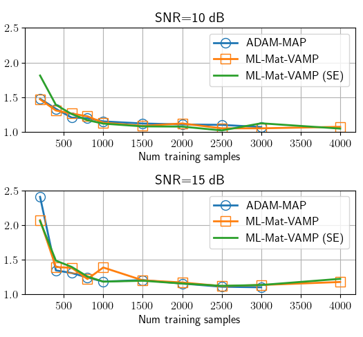
Fig. 2: Test error in learning the first layer of a 2 layer neural network using ADAM-based gradient descent, ML-Mat-VAMP and its state evolution prediction.

We consider the problem of learning the input layer of a two layer neural network as described in Section II-C. We learn the weights 𝑭1\bm{F}_{1} of the first layer of a two-layer network by solving problem (12). The LSL analysis in this case corresponds to the input size ninn_{\rm in} and number of samples NN going to infinity with the number of hidden units being fixed. Our experiment take d=4d=4 hidden units, Nin=100N_{\rm in}=100 input units, Nout=1N_{\rm out}=1 output unit, sigmoid activations and variable number of samples NN. The weight vectors 𝑭1\bm{F}_{1} and 𝑭2\bm{F}_{2} are generated as i.i.d. Gaussians with zero mean and unit variance. The input 𝐗\mathbf{X} is also i.i.d. Gaussians with variance 1/Nin1/N_{\rm in} so that the average pre-activation has unit variance. Output noise is added at two levels of 10 and 15 dB relative to the mean. We generate 1000 test samples and a variable number of training samples that ranges from 200 to 4000. For each trial and number of training samples, we compare three methods: (i) MAP estimation where the MAP loss function is minimized by the ADAM optimizer [47] in the Keras package of Tensorflow; (ii) the M-VAMP algorithm run for 20 iterations and (iii) the M-VAMP state evolution prediction. The MAP-ADAM algorithm is run for 100 epochs with a learning rate =0.01=0.01. The expectations in the M-VAMP SE are estimated via Monte-Carlo sampling (hence there is some variation).

Given an estimate 𝐅^1\widehat{\mathbf{F}}_{1} and true value 𝐅10\mathbf{F}_{1}^{0}, we can compute the test error as follows: Given a new sample 𝐱\mathbf{x}, the true and predicted pre-activations will be 𝐳1=(𝐅10)T​𝐱\mathbf{z}_{1}=(\mathbf{F}_{1}^{0})^{\text{\sf T}}\mathbf{x} and 𝐳^1=𝐅^1T​𝐱\widehat{\mathbf{z}}_{1}=\widehat{\mathbf{F}}_{1}^{\text{\sf T}}\mathbf{x}. Thus, if the new sample 𝐱∼𝒩⁡(0,1Nin​𝐈)\mathbf{x}\sim{\mathcal{N}}(0,\tfrac{1}{N_{\rm in}}\mathbf{I}), the true and predicted pre-activations, (𝐳1,𝐳^1)(\mathbf{z}_{1},\widehat{\mathbf{z}}_{1}), will be jointly Gaussian with covaraince equal to the empirical 2​d×2​d2d\times 2d covariance matrix of the rows of 𝐅10\mathbf{F}_{1}^{0} and 𝐅^1\widehat{\mathbf{F}}_{1}:

𝐊:=1Nin∑k=1Nin𝐮kT𝐮k,𝐮k=[𝐅1,k:𝐅^1,k:]\mathbf{K}:=\tfrac{1}{N_{\rm in}}\sum_{k=1}^{N_{\rm in}}\mathbf{u}_{k}^{\text{\sf T}}\mathbf{u}_{k},\quad\mathbf{u}_{k}=\left[\mathbf{F}_{1,k:}~\widehat{\mathbf{F}}_{1,k:}\right] (26)

From this covariance matrix, we can estimate the test error,

𝔼|y−y^|2=𝔼|𝐅2T(σ(𝐳1)−σ(𝐳^1)|2,\mathbb{E}|y-\widehat{y}|^{2}=\mathbb{E}|\mathbf{F}_{2}^{\text{\sf T}}(\sigma(\mathbf{z}_{1})-\sigma(\widehat{\mathbf{z}}_{1})|^{2},

where the expectation is taken over the Gaussian (𝐳1,𝐳^1)(\mathbf{z}_{1},\widehat{\mathbf{z}}_{1}) with covariance 𝐊\mathbf{K}. Also, since (26) is a row-wise operation, it can be predicted from the ML-Mat-VAMP SE. Thus, the SE can also predict the asymptotic test error. The normalized test error for ADAM-MAP, ML-Mat-VAMP and the ML-Mat-VAMP SE are plotted in Fig. 2. The normalized test error is defined as the ratio of the MSE on the test samples to the optimal MSE. Hence, a normalized MSE of one is the minimum value.

Note that since ADAM and ML-Mat-VAMP are solving the same optimization problem, they perform similarly as expected. The main message of this paper is not to develop an algorithm that outperforms ADAM, but rather an algorithm that has theoretical guarantees. The key property of ML-Mat-VAMP is that its asymptotic behavior at all the iterations can be exactly predicted by the state evolution equations. In this example, Fig. 2 shows tat the normalized test MSE predicted via state evolution (plotted in green) matches the normalized MSE of ML-Mat-VAMP estimates (plotted in orange).

Conclusions

We have developed a general framework for analyzing inference in multi-layer networks with matrix valued quantities in certain high-dimensional random settings. For learning the input layer of a two layer network, the methods enables precise predictions of the expected test error as a function of the parameter statistics, numbers of samples and noise level. This analysis can thus in turn be valuable in understanding key properties such as generalization error. Future work will look to extend these to more complex networks.

Acknowledgements

The work of P. Schniter was supported by NSF grant 1716388. The work of P. Pandit, M. Saharee-Ardakan and A. K. Fletcher was supported in part by the NSF Grants 1738285 and 1738286, ONR Grant N00014-15-1-2677. The work of S. Rangan was supported in part by NSF grants 1116589, 1302336, and 1547332, NIST, SRC and the the industrial affiliates of NYU Wireless.

Appendix A State Evolution Equations

Algorithm 2 State Evolution for ML-Mat-VAMP (Algo. 1)
0:   Functions {fℓ0}\{f^{0}_{\ell}\} from (28), {hℓ±}\{h_{\ell}^{\pm}\} from (29), and {fℓ±}\{f^{\pm}_{\ell}\} from (30). Perturbation random variables {Wℓ}\{W_{\ell}\} from (27). Initial random vectors {Q0​ℓ−}ℓ=0L−1\{Q_{0\ell}^{-}\}_{\ell=0}^{L-1} with Initial covariance matrices {𝝉0​ℓ−}ℓ=0L−1\{{\bm{\tau}}_{0\ell}^{-}\}_{\ell=0}^{L-1} from (21). Initial matrices {𝚪¯0​ℓ−}ℓ=0L\{\overline{\mathbf{\Gamma}}_{0\ell}^{-}\}_{\ell=0}^{L} from (22).
1:  // Initial Pass
2:  Q00=W0Q^{0}_{0}=W_{0}, 𝝉00=Cov⁡(Q00){\bm{\tau}}^{0}_{0}=\mathrm{Cov}(Q^{0}_{0}) and P00∼𝒩⁡(𝟎,𝝉00)P^{0}_{0}\sim{\mathcal{N}}(\mathbf{0},{\bm{\tau}}^{0}_{0})
3:  for ℓ=1,…,L−1\ell=1,\ldots,L\!-\!1 do
4:   Qℓ0=fℓ0​(Pℓ−10,Wℓ)Q^{0}_{\ell}=f^{0}_{\ell}(P^{0}_{\ell\!-\!1},W_{\ell})
5:   Pℓ0∼𝒩⁡(𝟎,𝝉ℓ0)P^{0}_{\ell}\sim{\mathcal{N}}(\mathbf{0},{\bm{\tau}}^{0}_{\ell}),  𝝉ℓ0=Cov⁡(Qℓ0){\bm{\tau}}^{0}_{\ell}=\mathrm{Cov}(Q^{0}_{\ell})
6:  end for
7:  for k=0,1,…k=0,1,\ldots do
8:   // Forward Pass
9:   Q^k​0+=h0+​(Qk​0−,W0,𝚯¯k​0+)\widehat{Q}^{+}_{k0}=h^{+}_{0}(Q_{k0}^{-},W_{0},\overline{\mathbf{\Theta}}^{+}_{k0})
10:   𝚲¯k​0+=(𝔼​∂Q^k​0+∂Q0−)−1​𝚪¯k,0−\overline{\mathbf{\Lambda}}_{k0}^{+}=(\mathbb{E}\tfrac{\partial\widehat{Q}^{+}_{k0}}{\partial Q_{0}^{-}})^{-1}\overline{\mathbf{\Gamma}}_{k,0}^{-}
11:   𝚪¯k​0+=𝚲¯k​0+−𝚪¯k​0−\overline{\mathbf{\Gamma}}_{k0}^{+}=\overline{\mathbf{\Lambda}}_{k0}^{+}-\overline{\mathbf{\Gamma}}_{k0}^{-}
12:   Qk​0+=f0+​(Qk​0−,W0,𝛀¯k​0+)Q_{k0}^{+}=f^{+}_{0}(Q_{k0}^{-},W_{0},\overline{\mathbf{\Omega}}^{+}_{k0})
13:   (P00,Pk​0+)∼𝒩⁡(𝟎,𝐊k​0+)(P^{0}_{0},P_{k0}^{+})\sim{\mathcal{N}}(\mathbf{0},\mathbf{K}_{k0}^{+}), 𝐊k​0+:=Cov⁡(Q00,Qk​0+)\qquad\mathbf{K}_{k0}^{+}:=\mathrm{Cov}(Q^{0}_{0},Q_{k0}^{+})
14:   for ℓ=1,…,L−1\ell=1,\ldots,L-1 do
15:    Q^k​ℓ+=hℓ+​(Pℓ−10,Pk,ℓ−1+,Qk​ℓ−,Wℓ,𝚯¯k​ℓ+)\widehat{Q}^{+}_{k\ell}=h^{+}_{\ell}(P^{0}_{\ell\!-\!1},P^{+}_{k,\ell\!-\!1},Q_{k\ell}^{-},W_{\ell},\overline{\mathbf{\Theta}}^{+}_{k\ell})
16:    𝚲¯k​ℓ+=(𝔼​∂Q^k​ℓ+∂Qk​ℓ−)−1​𝚪¯k​ℓ−\overline{\mathbf{\Lambda}}_{k\ell}^{+}=(\mathbb{E}\tfrac{\partial\widehat{Q}^{+}_{k\ell}}{\partial Q_{k\ell}^{-}})^{-1}\overline{\mathbf{\Gamma}}_{k\ell}^{-}
17:    𝚪¯k​ℓ+=𝚲¯k​ℓ+−𝚪¯k​ℓ−\overline{\mathbf{\Gamma}}_{k\ell}^{+}=\overline{\mathbf{\Lambda}}_{k\ell}^{+}-\overline{\mathbf{\Gamma}}_{k\ell}^{-}
18:    Qk​ℓ+=fℓ+​(Pℓ−10,Pk,ℓ−1+,Qk​ℓ−,Wℓ,𝛀¯k​ℓ+)Q_{k\ell}^{+}=f^{+}_{\ell}(P^{0}_{\ell\!-\!1},P^{+}_{k,\ell\!-\!1},Q_{k\ell}^{-},W_{\ell},\overline{\mathbf{\Omega}}^{+}_{k\ell})
19:    (Pℓ0,Pk​ℓ+)∼𝒩⁡(𝟎,𝐊k​ℓ+)(P^{0}_{\ell},P_{k\ell}^{+})\sim{\mathcal{N}}(\mathbf{0},\mathbf{K}_{k\ell}^{+}), 𝐊k​ℓ+:=Cov⁡(Qℓ0,Qk​ℓ+)\quad\mathbf{K}_{k\ell}^{+}:=\mathrm{Cov}(Q^{0}_{\ell},Q_{k\ell}^{+})
20:   end for
21:   // Backward Pass
22:   P^k+1,L−1−=hL−​(PL−10,Pk,L−1+,WL,𝚯¯k+1,L−)\widehat{P}_{k\!+\!1,L\!-\!1}^{-}=h^{-}_{L}(P^{0}_{L\!-\!1},P_{k,L\!-\!1}^{+},{W_{L}},\overline{\mathbf{\Theta}}^{-}_{k\!+\!1,L})
23:   𝚲¯k+1,L−=(𝔼​∂P^k+1,L−1−∂PL−1+)−1​𝚪¯k​L+\overline{\mathbf{\Lambda}}_{k+1,L}^{-}=(\mathbb{E}\tfrac{\partial\widehat{P}_{k\!+\!1,L\!-\!1}^{-}}{\partial P_{L\!-\!1}^{+}})^{-1}\overline{\mathbf{\Gamma}}_{kL}^{+}
24:   𝚪¯k+1,L−1−=𝚲¯k+1,L−1−−𝚪¯k,L−1+,\overline{\mathbf{\Gamma}}_{k+1,L\!-\!1}^{-}=\overline{\mathbf{\Lambda}}_{k+1,L\!-\!1}^{-}-\overline{\mathbf{\Gamma}}_{k,L\!-\!1}^{+},
25:   Pk+1,L−1−=fL−​(PL−10,Pk,L−1+,WL,𝛀¯k+1,L−)P_{k\!+\!1,L\!-\!1}^{-}=f^{-}_{L}(P^{0}_{L\!-\!1},P_{k,L\!-\!1}^{+},W_{L},\overline{\mathbf{\Omega}}^{-}_{k\!+\!1,L})
26:   Qk+1,L−1−∼𝒩⁡(𝟎,𝝉k+1,L−1−),Q_{k\!+\!1,L\!-\!1}^{-}\sim{\mathcal{N}}(\mathbf{0},{\bm{\tau}}_{k\!+\!1,L\!-\!1}^{-}),𝝉k+1,L−1−:=Cov⁡(Pk+1,L−1−)\ \ {\bm{\tau}}_{k\!+\!1,L\!-\!1}^{-}:=\mathrm{Cov}(P^{-}_{k\!+\!1,L\!-\!1})
27:   for ℓ=L−2,…,0\ell=L\!-\!2,\ldots,0 do
28:    P^k+1,ℓ−=hℓ−​(Pℓ0,Pk​ℓ+,Qk+1,ℓ+1−,Wℓ,𝚯¯k+1,ℓ−)\widehat{P}_{k\!+\!1,\ell}^{-}=h^{-}_{\ell}(P^{0}_{\ell},P_{k\ell}^{+},Q^{-}_{k+1,\ell+1},W_{\ell},\overline{\mathbf{\Theta}}^{-}_{k\!+\!1,\ell})
29:    𝚲¯k+1,ℓ−=(𝔼​∂P^k+1,ℓ−∂Pk,ℓ+)−1​𝚪¯k,ℓ+\overline{\mathbf{\Lambda}}_{k+1,\ell}^{-}=(\mathbb{E}\tfrac{\partial\widehat{P}_{k\!+\!1,\ell}^{-}}{\partial P_{k,\ell}^{+}})^{-1}\overline{\mathbf{\Gamma}}_{k,\ell}^{+}
30:    𝚪¯k+1,ℓ−=𝚲¯k+1,ℓ−−𝚪¯k,ℓ+,\overline{\mathbf{\Gamma}}_{k+1,\ell}^{-}=\overline{\mathbf{\Lambda}}_{k+1,\ell}^{-}-\overline{\mathbf{\Gamma}}_{k,\ell}^{+},
31:    Pk+1,ℓ−=fℓ−​(Pℓ0,Pk​ℓ+,Qk+1,ℓ+1−,Wℓ,𝛀¯k+1,ℓ−)P_{k\!+\!1,\ell}^{-}=f^{-}_{\ell}(P^{0}_{\ell},P^{+}_{k\ell},Q_{k\!+\!1,\ell+1}^{-},W_{\ell},\overline{\mathbf{\Omega}}^{-}_{k+1,\ell})
32:    Qk+1,ℓ−∼𝒩⁡(𝟎,𝝉k+1,ℓ−),Q_{k\!+\!1,\ell}^{-}\sim{\mathcal{N}}(\mathbf{0},{\bm{\tau}}_{k\!+\!1,\ell}^{-}), 𝝉k+1,ℓ−:=Cov⁡(Pk+1,ℓ−)\quad{\bm{\tau}}_{k\!+\!1,\ell}^{-}:=\mathrm{Cov}(P_{k\!+\!1,\ell}^{-})
33:   end for
34:  end for

The state evolution equations given in Algo. 2 define an iteration indexed by kk of constant matrices {𝐊k​ℓ+,𝝉k​l−,𝚪¯k​l±}ℓ=0L.\{\mathbf{K}_{k\ell}^{+},{\bm{\tau}}_{kl}^{-},\overline{\mathbf{\Gamma}}_{kl}^{\pm}\}_{\ell=0}^{L}. These constants appear in the statement of the main result in Theorem 1. The iterations in Algo. 2 also iteratively define a few ℝ1×d\mathbb{R}^{1\times d} valued random vectors {Qℓ0,Pℓ0,Qk​ℓ±,Pk​ℓ±}\{Q_{\ell}^{0},P_{\ell}^{0},Q_{k\ell}^{\pm},P_{k\ell}^{\pm}\} which are either multivariate Gaussian or functions of Multivariate Gaussians. In order to state Algorithm 2, we need to define certain random variables and functions appearing therein which are described below. Let ℒodd={1,3,…,L−1}\mathcal{L}_{\rm odd}=\{1,3,\ldots,L-1\} and ℒeven={2,4,…,L−2}\mathcal{L}_{\rm even}=\{2,4,\ldots,L-2\}.

Define {𝚯¯k​ℓ±}\{\overline{\mathbf{\Theta}}_{k\ell}^{\pm}\} similar to 𝚯k​ℓ±{\bm{\Theta}}_{k\ell}^{\pm} from equation (17) using {𝚪¯k​ℓ±}\{\overline{\mathbf{\Gamma}}_{k\ell}^{\pm}\}. Further, for ℓ=1,2,…,L−1\ell=1,2,\ldots,L-1 define

𝛀¯k​ℓ+:=(𝚲¯k​ℓ+,𝚪¯k​ℓ+,𝚪¯k​ℓ−),𝛀¯k​ℓ−:=(𝚲¯k,ℓ−1+,𝚪¯k,ℓ−1−,𝚪¯k,ℓ−1−),\overline{\mathbf{\Omega}}_{k\ell}^{+}:=(\overline{\mathbf{\Lambda}}_{k\ell}^{+},\overline{\mathbf{\Gamma}}_{k\ell}^{+},\overline{\mathbf{\Gamma}}_{k\ell}^{-}),\ \overline{\mathbf{\Omega}}_{k\ell}^{-}:=(\overline{\mathbf{\Lambda}}_{k,\ell-1}^{+},\overline{\mathbf{\Gamma}}_{k,\ell-1}^{-},\overline{\mathbf{\Gamma}}_{k,\ell-1}^{-}),

and 𝛀¯k​0+\overline{\mathbf{\Omega}}_{k0}^{+} and 𝛀¯k​L−.\overline{\mathbf{\Omega}}_{kL}^{-}. Now define random variables WℓW_{\ell} as

W0=Z00,WL=(Y,ΞL),Wℓ=Ξℓ,\displaystyle W_{0}=Z_{0}^{0},\ \ W_{L}=(Y,\Xi_{L}),\ \ W_{\ell}=\Xi_{\ell}, ∀ℓ∈ℒeven,\displaystyle\forall\,\ell\in\mathcal{L}_{\rm even}, (27)
Wℓ=(Sℓ,B¯ℓ,Ξℓ),\displaystyle W_{\ell}=(S_{\ell},\overline{B}_{\ell},\Xi_{\ell}), ∀ℓ∈ℒodd.\displaystyle\forall\,\ell\in\mathcal{L}_{\rm odd}.

Define functions {fℓ0}ℓ=1L\{f_{\ell}^{0}\}_{\ell=1}^{L} as

f0ℓ(P0ℓ−1,Wℓ):=SℓP0ℓ−1+B¯ℓ+Ξℓ,∀ℓ∈ℒodd,\displaystyle f^{0}_{\ell}(P^{0}_{\ell\!-\!1},W_{\ell}):={S}_{\ell}P^{0}_{\ell-1}+\overline{B}_{\ell}+{\Xi}_{\ell},\quad\forall\,\ell\in\mathcal{L}_{\rm odd}, (28)
f0ℓ(P0ℓ−1,Wℓ):=ϕℓ(P0ℓ−1,Ξℓ),∀ℓ∈ℒeven∪{L}.\displaystyle f^{0}_{\ell}(P^{0}_{\ell\!-\!1},W_{\ell}):=\phi_{\ell}(P^{0}_{\ell\!-\!1},\Xi_{\ell}),\quad\forall\,\ell\in\mathcal{L}_{\rm even}\cup\{L\}.

and using (17) define functions {hℓ±,}ℓ=1L\{h_{\ell}^{\pm},\}_{\ell=1}^{L}, h0+h_{0}^{+} and hL−h_{L}^{-} as

hℓ±​(Pℓ−10,Pℓ−1+,Qℓ−,Wℓ,𝚯k​ℓ±)\displaystyle h_{\ell}^{\pm}(P_{\ell-1}^{0},P_{\ell-1}^{+},Q_{\ell}^{-},W_{\ell},{\bm{\Theta}}_{k\ell}^{\pm}) (29)
=Gℓ±(Qℓ−+Qℓ0,Pℓ−1++Pℓ−10,𝚯k​ℓ±),∀ℓ∈ℒeven,\displaystyle=G_{\ell}^{\pm}(Q_{\ell}^{-}+Q_{\ell}^{0},P_{\ell-1}^{+}+P_{\ell-1}^{0},{\bm{\Theta}}_{k\ell}^{\pm}),\ \ \forall\,\ell\in\mathcal{L}_{\rm even},
hℓ±​(Pℓ−10,Pℓ−1+,Qℓ−,Wℓ,𝚯k​ℓ±)\displaystyle h_{\ell}^{\pm}(P_{\ell-1}^{0},P_{\ell-1}^{+},Q_{\ell}^{-},W_{\ell},{\bm{\Theta}}_{k\ell}^{\pm})
=G~ℓ±​(Qℓ−+Qℓ0,Pℓ−1++Pℓ−10,𝚯k​ℓ±),∀ℓ∈ℒodd\displaystyle=\widetilde{G}_{\ell}^{\pm}(Q_{\ell}^{-}+Q_{\ell}^{0},P_{\ell-1}^{+}+P_{\ell-1}^{0},{\bm{\Theta}}_{k\ell}^{\pm}),\ \ \forall\,\ell\in\mathcal{L}_{\rm odd}
h0+​(Q0−,W0,𝚯k​0+)=G0+​(Q0−+W0,𝚯k​0+),\displaystyle h_{0}^{+}(Q_{0}^{-},W_{0},{\bm{\Theta}}_{k0}^{+})=G^{+}_{0}(Q_{0}^{-}+W_{0},{\bm{\Theta}}_{k0}^{+}),
hL−​(PL−10,PL−1+,WL,𝚯k​L−)=GL−​(PL−1++PL−10,𝚯k​L−).\displaystyle h_{\mathchoice{\raisebox{0.0pt}{\resizebox{300660}{262144}{\hbox{\raisebox{0.0pt}{$\displaystyle L$}}}}}{\raisebox{0.0pt}{\resizebox{300660}{262144}{\hbox{\raisebox{0.0pt}{$\textstyle L$}}}}}{\raisebox{0.0pt}{\resizebox{261078}{262144}{\hbox{\raisebox{0.0pt}{$\scriptstyle L$}}}}}{\raisebox{0.0pt}{\resizebox{261078}{262144}{\hbox{\raisebox{0.0pt}{$\scriptscriptstyle L$}}}}}}^{-}(P_{\mathchoice{\raisebox{0.0pt}{\resizebox{866372}{262144}{\hbox{\raisebox{0.0pt}{$\displaystyle L-1$}}}}}{\raisebox{0.0pt}{\resizebox{866372}{262144}{\hbox{\raisebox{0.0pt}{$\textstyle L-1$}}}}}{\raisebox{0.0pt}{\resizebox{865899}{262144}{\hbox{\raisebox{0.0pt}{$\scriptstyle L-1$}}}}}{\raisebox{0.0pt}{\resizebox{979952}{262144}{\hbox{\raisebox{0.0pt}{$\scriptscriptstyle L-1$}}}}}}^{0},P_{\mathchoice{\raisebox{0.0pt}{\resizebox{866372}{262144}{\hbox{\raisebox{0.0pt}{$\displaystyle L-1$}}}}}{\raisebox{0.0pt}{\resizebox{866372}{262144}{\hbox{\raisebox{0.0pt}{$\textstyle L-1$}}}}}{\raisebox{0.0pt}{\resizebox{865899}{262144}{\hbox{\raisebox{0.0pt}{$\scriptstyle L-1$}}}}}{\raisebox{0.0pt}{\resizebox{979952}{262144}{\hbox{\raisebox{0.0pt}{$\scriptscriptstyle L-1$}}}}}}^{+},W_{\mathchoice{\raisebox{0.0pt}{\resizebox{300660}{262144}{\hbox{\raisebox{0.0pt}{$\displaystyle L$}}}}}{\raisebox{0.0pt}{\resizebox{300660}{262144}{\hbox{\raisebox{0.0pt}{$\textstyle L$}}}}}{\raisebox{0.0pt}{\resizebox{261078}{262144}{\hbox{\raisebox{0.0pt}{$\scriptstyle L$}}}}}{\raisebox{0.0pt}{\resizebox{261078}{262144}{\hbox{\raisebox{0.0pt}{$\scriptscriptstyle L$}}}}}},{\bm{\Theta}}_{{\mathchoice{\raisebox{0.0pt}{\resizebox{534216}{262143}{\hbox{\raisebox{0.0pt}{$\displaystyle kL$}}}}}{\raisebox{0.0pt}{\resizebox{534216}{262143}{\hbox{\raisebox{0.0pt}{$\textstyle kL$}}}}}{\raisebox{0.0pt}{\resizebox{465305}{262144}{\hbox{\raisebox{0.0pt}{$\scriptstyle kL$}}}}}{\raisebox{0.0pt}{\resizebox{465306}{262144}{\hbox{\raisebox{0.0pt}{$\scriptscriptstyle kL$}}}}}}}^{-})=G^{-}_{\mathchoice{\raisebox{0.0pt}{\resizebox{300660}{262144}{\hbox{\raisebox{0.0pt}{$\displaystyle L$}}}}}{\raisebox{0.0pt}{\resizebox{300660}{262144}{\hbox{\raisebox{0.0pt}{$\textstyle L$}}}}}{\raisebox{0.0pt}{\resizebox{261078}{262144}{\hbox{\raisebox{0.0pt}{$\scriptstyle L$}}}}}{\raisebox{0.0pt}{\resizebox{261078}{262144}{\hbox{\raisebox{0.0pt}{$\scriptscriptstyle L$}}}}}}(P_{\mathchoice{\raisebox{0.0pt}{\resizebox{1082965}{327680}{\hbox{\raisebox{0.0pt}{$\displaystyle L-1$}}}}}{\raisebox{0.0pt}{\resizebox{1082965}{327680}{\hbox{\raisebox{0.0pt}{$\textstyle L-1$}}}}}{\raisebox{0.0pt}{\resizebox{1082374}{327680}{\hbox{\raisebox{0.0pt}{$\scriptstyle L-1$}}}}}{\raisebox{0.0pt}{\resizebox{1224940}{327680}{\hbox{\raisebox{0.0pt}{$\scriptscriptstyle L-1$}}}}}}^{+}+P^{0}_{\mathchoice{\raisebox{0.0pt}{\resizebox{1082965}{327680}{\hbox{\raisebox{0.0pt}{$\displaystyle L-1$}}}}}{\raisebox{0.0pt}{\resizebox{1082965}{327680}{\hbox{\raisebox{0.0pt}{$\textstyle L-1$}}}}}{\raisebox{0.0pt}{\resizebox{1082374}{327680}{\hbox{\raisebox{0.0pt}{$\scriptstyle L-1$}}}}}{\raisebox{0.0pt}{\resizebox{1224940}{327680}{\hbox{\raisebox{0.0pt}{$\scriptscriptstyle L-1$}}}}}},{\bm{\Theta}}_{{\mathchoice{\raisebox{0.0pt}{\resizebox{534216}{262143}{\hbox{\raisebox{0.0pt}{$\displaystyle kL$}}}}}{\raisebox{0.0pt}{\resizebox{534216}{262143}{\hbox{\raisebox{0.0pt}{$\textstyle kL$}}}}}{\raisebox{0.0pt}{\resizebox{465305}{262144}{\hbox{\raisebox{0.0pt}{$\scriptstyle kL$}}}}}{\raisebox{0.0pt}{\resizebox{465306}{262144}{\hbox{\raisebox{0.0pt}{$\scriptscriptstyle kL$}}}}}}}^{-}).

Note that [Gℓ+,Gℓ−][G_{\ell}^{+},G_{\ell}^{-}] and [G~ℓ+,G~ℓ−][\widetilde{G}_{\ell}^{+},\widetilde{G}_{\ell}^{-}] are maps from ℝ1×d→ℝ1×d\mathbb{R}^{1\times d}\rightarrow\mathbb{R}^{1\times d} such that their row-wise extensions are the denoisers [𝐆ℓ+,𝐆ℓ−][\mathbf{G}_{\ell}^{+},\mathbf{G}_{\ell}^{-}] and [𝐆~ℓ+,𝐆~ℓ−][\widetilde{\mathbf{G}}_{\ell}^{+},\widetilde{\mathbf{G}}_{\ell}^{-}] respectively. Using (29) define functions {fℓ±}ℓ=1L−1\{f_{\ell}^{\pm}\}_{\ell=1}^{L-1}, f0+f_{0}^{+} and fL−f_{L}^{-} as

fℓ+​(Pℓ−10,Pℓ−1+,Qℓ−,Wℓ,𝛀k​ℓ+)\displaystyle f^{+}_{\ell}(P^{0}_{\ell\!-\!1},P_{\ell\!-\!1}^{+},Q_{\ell}^{-},W_{\ell},\mathbf{\Omega}_{k\ell}^{+}) (30)
=[(hℓ+−Qℓ0)​𝚲k​ℓ+−Qℓ−​𝚪k​ℓ−]​(𝚪k​ℓ+)−1,\displaystyle=\left[\left(h^{+}_{\ell}-Q^{0}_{\ell}\right)\mathbf{\Lambda}_{k\ell}^{+}-Q_{\ell}^{-}{\bm{\Gamma}}_{k\ell}^{-}\right]({\bm{\Gamma}}_{k\ell}^{+})^{-1},
fℓ−​(Pℓ−10,Pℓ−1+,Qℓ−,Wℓ,𝛀k​ℓ−)\displaystyle f^{-}_{\ell}(P^{0}_{\ell\!-\!1},P_{\ell\!-\!1}^{+},Q_{\ell}^{-},W_{\ell},\mathbf{\Omega}_{k\ell}^{-})
=[(hℓ−−Pℓ−10)​𝚲k,ℓ−1−−Pℓ−1+​𝚪k,ℓ−1+]​(𝚪k,ℓ−1−)−1.\displaystyle=\left[\left(h^{-}_{\ell}-P^{0}_{\ell\!-\!1}\right)\mathbf{\Lambda}_{k,\ell\!-\!1}^{-}-P_{\ell\!-\!1}^{+}{\bm{\Gamma}}_{k,\ell\!-\!1}^{+}\right]({\bm{\Gamma}}_{k,\ell\!-\!1}^{-})^{-1}.
f0+​(Q0−,W0,𝛀k​0+)\displaystyle f^{+}_{0}(Q_{0}^{-},W_{0},\mathbf{\Omega}_{k0}^{+})
=[(h0+−W0)​𝚲k​0+−Q0−​𝚪k​0−]​(𝚪k​0+)−1,\displaystyle=\left[\left(h^{+}_{0}-W_{0}\right)\mathbf{\Lambda}_{k0}^{+}-Q_{0}^{-}{\bm{\Gamma}}_{k0}^{-}\right]({\bm{\Gamma}}_{k0}^{+})^{-1},
fL−​(PL−10,PL−1+,WL,𝛀k​L−)\displaystyle f^{-}_{L}(P^{0}_{L\!-\!1},P_{L\!-\!1}^{+},W_{L},\mathbf{\Omega}_{kL}^{-})
=[(hL−−PL−10)​𝚲k,L−1−−PL−1+​𝚪k,L−1+]​(𝚪k,L−1−)−1.\displaystyle=\left[\left(h^{-}_{L}-P^{0}_{L\!-\!1}\right)\mathbf{\Lambda}_{k,L\!-\!1}^{-}-P_{L\!-\!1}^{+}{\bm{\Gamma}}_{k,L\!-\!1}^{+}\right]({\bm{\Gamma}}_{k,L\!-\!1}^{-})^{-1}.

Appendix B Large System Limit Details

The analysis of Algorithm 1 in the large system limit is based on [21] and is by now standard in the theory of AMP-based algorithms. The goal is to characterize ensemble row-wise averages of iterates of the algorithm using simpler finite-dimensional random variables which are either Gaussians or functions of Gaussians. To that end, we start by defining some key terms needed in this analysis.

Definition 1 (Pseudo-Lipschitz continuity).

For a given p≥1p\geq 1, a map 𝐠:ℝ1×d→ℝ1×r\mathbf{g}:\mathbb{R}^{1\times d}\rightarrow\mathbb{R}^{1\times r} is called pseudo-Lipschitz of order pp if for any 𝐫1,𝐫2∈ℝd\mathbf{r}_{1},\mathbf{r}_{2}\in\mathbb{R}^{d} we have,

‖𝐠⁡(𝐫1)−𝐠⁡(𝐫2)‖≤C​‖𝐫1−𝐫2‖​(1+‖𝐫1‖p−1+‖𝐫2‖p−1)\displaystyle\|\mathbf{g}(\mathbf{r}_{1})-\mathbf{g}(\mathbf{r}_{2})\|\leq C\|\mathbf{r}_{1}-\mathbf{r}_{2}\|\left(1+\|\mathbf{r}_{1}\|^{p-1}+\|\mathbf{r}_{2}\|^{p-1}\right)
Definition 2 (Empirical convergence of rows of a matrix sequence).

Consider a matrix-sequence {𝐗(N)}N=1∞\{\mathbf{X}^{(N)}\}_{N=1}^{\infty} with 𝐗(N)∈ℝN×d.\mathbf{X}^{(N)}\in\mathbb{R}^{N\times d}. For a finite p≥1p\geq 1, let X∈(ℝd,ℛd)X\in(\mathbb{R}^{d},\mathcal{R}^{d}) be a ℛd\mathcal{R}^{d}-measurable random variable with bounded moment 𝔼​‖X‖pp<∞\mathbb{E}\|X\|_{p}^{p}<\infty. We say the rows of matrix sequence {𝐗(N)}\{\mathbf{X}^{(N)}\} converge empirically to XX with pt​hp^{th} order moments if for all pseudo-Lipschitz continuous functions f⁡(⋅)f(\cdot) of order pp,

limN→∞1N∑n=1Nf(𝐗n:(N))=𝔼[f(X)]a.s.\displaystyle\lim_{N\rightarrow\infty}\frac{1}{N}\sum_{n=1}^{N}f(\mathbf{X}^{(N)}_{n:})=\mathbb{E}[f(X)]\quad{\rm a.s.} (31)

Note that the sequence {𝐗(N)}\{\mathbf{X}^{(N)}\} could be random or deterministic. If it is random, however, then the quantities on the left hand side are random sums and the almost sure convergence must take this randomness into account as well.

The above convergence is equivalent to requiring weak convergence as well as convergence of the pthp^{\rm th} moment, of the empirical distribution 1N∑n=1Nδ𝐗n:(N)\tfrac{1}{N}\sum_{n=1}^{N}\delta_{\mathbf{X}_{n:}^{(N)}} of the rows of 𝐗(N)\mathbf{X}^{(N)} to XX. This is also referred to convergence in the Wasserstein-pp metric [48, Chap. 6].

In the case of p=2p=2, the condition is equivalent to requiring (31) to hold for all continuously bounded functions ff as well as for all fq​(𝒙)=𝒙T​𝑸​𝒙f_{q}(\bm{x})=\bm{x}^{\text{\sf T}}\bm{Q}\bm{x} for all positive definite matrices 𝑸\bm{Q}.

Definition 3 (Uniform Lipschitz continuity).

For a positive definite matrix 𝑴\bm{M}, the map ϕ⁡(𝐫,𝑴):ℝd→ℝd\phi(\mathbf{r};\bm{M}):\mathbb{R}^{d}\rightarrow\mathbb{R}^{d} is said to be uniformly Lipschitz continuous in 𝐫\mathbf{r} at 𝑴=𝑴¯\bm{M}=\overline{\bm{M}} if there exist non-negative constants L1L_{1}, L2L_{2} and L3L_{3} such that for all 𝐫∈ℝd\mathbf{r}\in\mathbb{R}^{d}

‖ϕ⁡(𝐫1,𝑴0)−ϕ⁡(𝐫2,𝑴0)‖\displaystyle\|\phi(\mathbf{r}_{1};\bm{M}_{0})-\phi(\mathbf{r}_{2};\bm{M}_{0})\| ≤L1​‖𝐫1−𝐫2‖\displaystyle\leq L_{1}\|\mathbf{r}_{1}-\mathbf{r}_{2}\|
‖ϕ⁡(𝐫,𝑴1)−ϕ⁡(𝐫,𝑴2)‖\displaystyle\|\phi(\mathbf{r};\bm{M}_{1})-\phi(\mathbf{r};\bm{M}_{2})\| ≤L2​(1+‖𝐫‖)​ρ​(𝑴1,𝑴2)\displaystyle\leq L_{2}(1+\|\mathbf{r}\|)\rho(\bm{M}_{1},\bm{M}_{2})

for all 𝑴i\bm{M}_{i} such that ρ⁡(𝑴i,𝑴¯)<L3\rho(\bm{M}_{i},\overline{\bm{M}})<L_{3} where ρ\rho is a metric on the cone of positive semidefinite matrices.

We are now ready to prove Theorem 1.

Appendix C Proof of Theorem 1

The proof of Theorem 1 is a special case of a more general result on multi-layer recursions given in Theorem 2. This result is stated in Appendix D, and proved in Appendix E. The rest of this section identifies certain relevant quantities from Theorem 1 in order to apply Theorem 2.

Consider the SVD given in equation (19) of weight matrices 𝐖ℓ\mathbf{W}_{\ell} of the network. We analyze Algo. 1 using transformed versions of the true signals 𝐙ℓ0\mathbf{Z}_{\ell}^{0} and input errors 𝐑ℓ±−𝐙ℓ0\mathbf{R}_{\ell}^{\pm}-\mathbf{Z}_{\ell}^{0} to the denoisers 𝐆ℓ±\mathbf{G}_{\ell}^{\pm}. For ℓ=0,2,…​L−2\ell=0,2,\ldots L-2, define

𝐪ℓ0=𝐙ℓ0\displaystyle\mathbf{q}_{\ell}^{0}=\mathbf{Z}_{\ell}^{0} 𝐪ℓ+10\displaystyle\mathbf{q}_{\ell+1}^{0} =𝐕ℓ+1⊤​𝐙ℓ+10\displaystyle=\mathbf{V}_{\ell+1}^{\top}\mathbf{Z}_{\ell+1}^{0} (32a)
𝐩ℓ0=𝐕ℓ​𝐙ℓ0\displaystyle\mathbf{p}_{\ell}^{0}=\mathbf{V}_{\ell}\mathbf{Z}_{\ell}^{0} 𝐩ℓ+10\displaystyle\mathbf{p}_{\ell+1}^{0} =𝐙ℓ+10\displaystyle=\mathbf{Z}_{\ell+1}^{0} (32b)

which are depicted in Fig. 3 (TOP). Similarly, define the following transformed versions of errors in the inputs 𝐑ℓ±\mathbf{R}_{\ell}^{\pm} to the denoisers 𝐆ℓ±\mathbf{G}_{\ell}^{\pm}

𝐪ℓ−=𝐑ℓ−−𝐙ℓ0\displaystyle\mathbf{q}_{\ell}^{-}=\mathbf{R}_{\ell}^{-}-\mathbf{Z}_{\ell}^{0} 𝐪ℓ+1−\displaystyle\mathbf{q}_{\ell+1}^{-} =𝐕ℓ+1⊤​(𝐑ℓ+1−−𝐙ℓ+10)\displaystyle=\mathbf{V}_{\ell+1}^{\top}(\mathbf{R}_{\ell+1}^{-}-\mathbf{Z}_{\ell+1}^{0}) (33a)
𝐩ℓ+=𝐕ℓ​(𝐑ℓ+−𝐙ℓ0)\displaystyle\mathbf{p}_{\ell}^{+}=\mathbf{V}_{\ell}(\mathbf{R}_{\ell}^{+}-\mathbf{Z}_{\ell}^{0}) 𝐩ℓ+1+\displaystyle\mathbf{p}_{\ell+1}^{+} =𝐑ℓ+1+−𝐙ℓ+10\displaystyle=\mathbf{R}_{\ell+1}^{+}-\mathbf{Z}_{\ell+1}^{0} (33b)

These quantities are depicted as inputs to function blocks 𝐟ℓ±\mathbf{f}_{\ell}^{\pm} in Fig. 3 (MIDDLE). Define perturbation variables 𝐰ℓ\mathbf{w}_{\ell} as

𝐰0\displaystyle\mathbf{w}_{0} =𝐙00,𝐰L=(𝐘,𝚵L),𝐰ℓ=𝚵ℓ,\displaystyle=\mathbf{Z}^{0}_{0},\ \ \mathbf{w}_{\mathchoice{\raisebox{0.0pt}{\resizebox{300660}{262144}{\hbox{\raisebox{0.0pt}{$\displaystyle L$}}}}}{\raisebox{0.0pt}{\resizebox{300660}{262144}{\hbox{\raisebox{0.0pt}{$\textstyle L$}}}}}{\raisebox{0.0pt}{\resizebox{261078}{262144}{\hbox{\raisebox{0.0pt}{$\scriptstyle L$}}}}}{\raisebox{0.0pt}{\resizebox{261078}{262144}{\hbox{\raisebox{0.0pt}{$\scriptscriptstyle L$}}}}}}=(\mathbf{Y},{\bm{\Xi}}_{\mathchoice{\raisebox{0.0pt}{\resizebox{300660}{262144}{\hbox{\raisebox{0.0pt}{$\displaystyle L$}}}}}{\raisebox{0.0pt}{\resizebox{300660}{262144}{\hbox{\raisebox{0.0pt}{$\textstyle L$}}}}}{\raisebox{0.0pt}{\resizebox{261078}{262144}{\hbox{\raisebox{0.0pt}{$\scriptstyle L$}}}}}{\raisebox{0.0pt}{\resizebox{261078}{262144}{\hbox{\raisebox{0.0pt}{$\scriptscriptstyle L$}}}}}}),\ \ \mathbf{w}_{\ell}={\bm{\Xi}}_{\ell}, ∀ℓ∈ℒeven\displaystyle\forall\,\ell\in\mathcal{L}_{\rm even} (34a)
𝐰ℓ\displaystyle\mathbf{w}_{\ell} =(𝐒ℓ,𝐁¯ℓ,𝚵ℓ),\displaystyle=(\mathbf{S}_{\ell},\overline{\mathbf{B}}_{\ell},{\bm{\Xi}}_{\ell}), ∀ℓ∈ℒodd\displaystyle\forall\,\ell\in\mathcal{L}_{\rm odd} (34b)

Finally, we define 𝐪ℓ+\mathbf{q}_{\ell}^{+} and 𝐩ℓ−\mathbf{p}_{\ell}^{-} for ℓ=1,2,…,L−1\ell=1,2,\ldots,L-1 as

𝐪ℓ+\displaystyle\mathbf{q}_{\ell}^{+} =𝐟ℓ+​(𝐩ℓ−10,𝐩ℓ−1+,𝐪ℓ−,𝐰ℓ,Ωℓ)\displaystyle=\mathbf{f}_{\ell}^{+}(\mathbf{p}_{\ell-1}^{0},\mathbf{p}_{\ell-1}^{+},\mathbf{q}_{\ell}^{-},\mathbf{w}_{\ell},\Omega_{\ell}) (35a)
𝐩ℓ−1−\displaystyle\mathbf{p}_{\ell\!-\!1}^{-} =𝐟ℓ−​(𝐩ℓ−10,𝐩ℓ−1+,𝐪ℓ−,𝐰ℓ,Ωℓ),\displaystyle=\mathbf{f}_{\ell}^{-}(\mathbf{p}_{\ell-1}^{0},\mathbf{p}_{\ell-1}^{+},\mathbf{q}_{\ell}^{-},\mathbf{w}_{\ell},\Omega_{\ell}), (35b)

which are outputs of function blocks in Fig. 3 (MIDDLE). Similarly, define the quantities 𝐪0+=𝐟0+​(𝐪0−,𝐙0,Ω0)\mathbf{q}_{0}^{+}=\mathbf{f}_{0}^{+}(\mathbf{q}_{0}^{-},\mathbf{Z}_{0},\Omega_{0}) and 𝐩L−1−=𝐟L+​(𝐩L−10,𝐩L−1+,𝐘,ΩL)\mathbf{p}_{L-1}^{-}=\mathbf{f}_{L}^{+}(\mathbf{p}_{L-1}^{0},\mathbf{p}_{L-1}^{+},\mathbf{Y},\Omega_{L}).

Lemma 1.

Algorithm 1 is a special case of Algorithm 3 with the definitions {𝐪ℓ0,𝐩ℓ0,𝐪ℓ±,𝐩ℓ±}ℓ=0L−1\{\mathbf{q}_{\ell}^{0},\mathbf{p}_{\ell}^{0},\mathbf{q}_{\ell}^{\pm},\mathbf{p}_{\ell}^{\pm}\}_{\ell=0}^{L-1} given in equations (32),(33), and (35), functions 𝐟ℓ±\mathbf{f}_{\ell}^{\pm} are row-wise extensions of fℓ±f_{\ell}^{\pm} defined using equations (30) and (29).

Lemma 2.

Assumptions 1 and 2 required for applying Theorem 2 are satisfied by the conditions in Theorem 1.

Proof.

The proofs of the above lemmas are identical to the case of d=1d=1, which was shown in [18]. For details see [18, Appendix F]. □\Box

Appendix D General Multi-Layer Recursions

𝐪0+\mathbf{q}^{+}_{0}𝐕0\mathbf{V}_{0}𝐕0\mathbf{V}_{0}𝐩00\mathbf{p}_{0}^{0}𝐟10\mathbf{f}_{1}^{0}𝐪00\mathbf{q}_{0}^{0}𝐩0+\mathbf{p}_{0}^{+}𝐟1−\mathbf{f}_{1}^{-}𝐩0−\mathbf{p}_{0}^{-}𝐕0⊤\mathbf{V}_{0}^{\top}𝒩\mathcal{N}P0+P_{0}^{+}P00P_{0}^{0}f1−f_{1}^{-}P0−P_{0}^{-}𝒩\mathcal{N}Q0−Q^{-}_{0}f0+f_{0}^{+}Q0+Q^{+}_{0}Q00Q^{0}_{0}𝐪0−\mathbf{q}^{-}_{0}𝐟0+\mathbf{f}_{0}^{+}𝐪1+\mathbf{q}^{+}_{1}𝐕1\mathbf{V}_{1}𝐕1\mathbf{V}_{1}𝐩10\mathbf{p}_{1}^{0}𝐟20\mathbf{f}_{2}^{0}𝐪10\mathbf{q}_{1}^{0}𝐩1+\mathbf{p}_{1}^{+}𝐟2−\mathbf{f}_{2}^{-}𝐩1−\mathbf{p}_{1}^{-}𝐕1⊤\mathbf{V}_{1}^{\top}𝒩\mathcal{N}P1+P_{1}^{+}P10P_{1}^{0}f2−f_{2}^{-}P1−P_{1}^{-}𝒩\mathcal{N}Q1−Q^{-}_{1}f1+f_{1}^{+}Q1+Q^{+}_{1}Q10Q^{0}_{1}𝐪1−\mathbf{q}^{-}_{1}𝐟1+\mathbf{f}_{1}^{+}𝐪2+\mathbf{q}^{+}_{2}𝐕2\mathbf{V}_{2}𝐕2\mathbf{V}_{2}𝐩20\mathbf{p}_{2}^{0}𝐟30\mathbf{f}_{3}^{0}𝐪20\mathbf{q}_{2}^{0}𝐩2+\mathbf{p}_{2}^{+}𝐟3−\mathbf{f}_{3}^{-}𝐩2−\mathbf{p}_{2}^{-}𝐕2⊤\mathbf{V}_{2}^{\top}𝒩\mathcal{N}P2+P_{2}^{+}P20P_{2}^{0}f3−f_{3}^{-}P2−P_{2}^{-}𝒩\mathcal{N}Q2−Q^{-}_{2}f2+f_{2}^{+}Q2+Q^{+}_{2}Q20Q^{0}_{2}𝐪2−\mathbf{q}^{-}_{2}𝐟2+\mathbf{f}_{2}^{+}𝐪3+\mathbf{q}^{+}_{3}𝐕3\mathbf{V}_{3}𝐕3\mathbf{V}_{3}𝐩30\mathbf{p}_{3}^{0}𝐪30\mathbf{q}_{3}^{0}𝐩3+\mathbf{p}_{3}^{+}𝐟4−\mathbf{f}_{4}^{-}𝐩3−\mathbf{p}_{3}^{-}𝐕3⊤\mathbf{V}_{3}^{\top}𝒩\mathcal{N}P3+P_{3}^{+}P30P_{3}^{0}f4−f_{4}^{-}P3−P_{3}^{-}𝒩\mathcal{N}Q3−Q^{-}_{3}f3+f_{3}^{+}Q3+Q^{+}_{3}Q30Q^{0}_{3}𝐪3−\mathbf{q}^{-}_{3}𝐟3+\mathbf{f}_{3}^{+}
Fig. 3: (TOP) The equations (1) with equivalent quantities defined in (32), and 𝐟ℓ0\mathbf{f}_{\ell}^{0} defined using (28).
(MIDDLE) The Gen-ML-Mat recursions in Algorithm 3. These are also equivalent to ML-Mat-VAMP recursions from Algorithm 1 (See Lemma 1) if 𝐪±,𝐩±\mathbf{q}^{\pm},\mathbf{p}^{\pm} are as defined as in equations (33) and (35), and 𝐟ℓ±\mathbf{f}_{\ell}^{\pm} given by equations (30) and (29).
(BOTTOM) Quantities in the GEN-ML-SE recursions. These are also equivalent to ML-Mat-VAMP SE recursions from Algorithm 2 (See Lemma 1)
The iteration indices kk have been dropped for notational simplicity.

To analyze Algorithm 1, we consider a more general class of recursions as given in Algorithm 3 and depicted in Fig. 3. The Gen-ML recursions generates (i) a set of true matrices 𝐪ℓ0\mathbf{q}_{\ell}^{0} and 𝐩ℓ0\mathbf{p}_{\ell}^{0} and (ii) iterated matrices 𝐪k​ℓ±\mathbf{q}^{\pm}_{k\ell} and 𝐩k​ℓ±\mathbf{p}^{\pm}_{k\ell}. Each of these matrices have the same number of columns, denoted by dd.

The true matrices are generated by a single forward pass, whereas the iterated matrices are generated via a sequence of forward and backward passes through a multi-layer system. In proving the State Evolution for the ML-Mat-VAMP algorithm (Algo. 1, one would then associate the terms 𝐪k​ℓ±\mathbf{q}^{\pm}_{k\ell} and 𝐩k​ℓ±\mathbf{p}^{\pm}_{k\ell} with certain error quantities in the ML-Mat-VAMP recursions. To account for the effect of the parameters 𝚪k​ℓ±{\bm{\Gamma}}^{\pm}_{k\ell} and 𝚲k​ℓ±\mathbf{\Lambda}^{\pm}_{k\ell} in ML-Mat-VAMP, the Gen-ML algorithm describes the parameter updates through a sequence of parameter lists Υk​ℓ±\Upsilon^{\pm}_{k\ell}. The parameter lists are ordered lists of parameters that accumulate as the algorithm progresses. The true and iterated matrices from Algorithm 3 are depicted in the signal flow graphs on the (TOP) and (MIDDLE) panel of Fig. 3 respectively. The iteration index kk for the iterated vectors 𝐪k​ℓ,𝐩k​ℓ\mathbf{q}_{k\ell},\mathbf{p}_{k\ell} has been dropped for simplifying notation.

The functions 𝐟ℓ0​(⋅)\mathbf{f}_{\ell}^{0}(\cdot) that produce the true matrices 𝐪ℓ0,𝐩ℓ0\mathbf{q}_{\ell}^{0},\mathbf{p}_{\ell}^{0} are called initial matrix functions and use the initial parameter list Υ01−\Upsilon_{01}^{-}. The functions 𝐟k​ℓ±​(⋅)\mathbf{f}_{k\ell}^{\pm}(\cdot) that produce the matrices 𝐪k​ℓ+\mathbf{q}^{+}_{k\ell} and 𝐩k​ℓ−\mathbf{p}^{-}_{k\ell} are called the matrix update functions and use parameter lists Υk​l±\Upsilon_{kl}^{\pm}. The initial parameter lists Υ01−\Upsilon^{-}_{01} are assumed to be provided. As the algorithm progresses, new parameters λk​ℓ±\lambda^{\pm}_{k\ell} are computed and then added to the lists in lines 12, 18, 25 and 31. The matrix update functions 𝐟k​ℓ±​(⋅)\mathbf{f}_{k\ell}^{\pm}(\cdot) may depend on any sets of parameters accumulated in the parameter list. In lines 11, 17, 24 and 30, the new parameters λk​ℓ±\lambda_{k\ell}^{\pm} are computed by: (1) computing average values μk​ℓ±\mu_{k\ell}^{\pm} of row-wise functions 𝝋k​ℓ±​(⋅){\bm{\varphi}}^{\pm}_{k\ell}(\cdot); and (2) taking functions Tk​ℓ±​(⋅)T^{\pm}_{k\ell}(\cdot) of the average values μk​ℓ±\mu_{k\ell}^{\pm}. Since the average values μk​ℓ±\mu_{k\ell}^{\pm} represent statistics on the rows of 𝝋k​ℓ±​(⋅){\bm{\varphi}}^{\pm}_{k\ell}(\cdot), we will call 𝝋k​ℓ±​(⋅){\bm{\varphi}}^{\pm}_{k\ell}(\cdot) the parameter statistic functions. We will call the Tk​ℓ±​(⋅)T^{\pm}_{k\ell}(\cdot) the parameter update functions. The functions 𝐟ℓ0,𝐟k​ℓ±,𝝋ℓ±\mathbf{f}_{\ell}^{0},\mathbf{f}_{k\ell}^{\pm},{\bm{\varphi}}^{\pm}_{\ell} also take as input some perturbation vectors 𝐰ℓ\mathbf{w}_{\ell}.

Algorithm 3 General Multi-Layer Matrix (Gen-ML-Mat) Recursion
0:  Initial matrix functions {𝐟ℓ0}\{\mathbf{f}_{\ell}^{0}\}. Matrix update functions {𝐟k​ℓ±​(⋅)}\{\mathbf{f}^{\pm}_{k\ell}(\cdot)\}. Parameter statistic functions {𝝋k​ℓ±​(⋅)}\{{\bm{\varphi}}^{\pm}_{k\ell}(\cdot)\}. Parameter update functions {Tk​ℓ±​(⋅)}\{T^{\pm}_{k\ell}(\cdot)\}. Orthogonal matrices {𝐕ℓ}\{\mathbf{V}_{\ell}\}. Perturbation variables {𝐰ℓ±}\{\mathbf{w}^{\pm}_{\ell}\}. Initial matrices {𝐪0​ℓ−}\{\mathbf{q}_{0\ell}^{-}\}. Initial parameter list Υ01−\Upsilon_{01}^{-}.
1:  // Initial Pass
2:  𝐪00=𝐟00​(𝐰0),𝐩00=𝐕0​𝐪00\mathbf{q}^{0}_{0}=\mathbf{f}^{0}_{0}(\mathbf{w}_{0}),\quad\mathbf{p}^{0}_{0}=\mathbf{V}_{0}\mathbf{q}^{0}_{0}
3:  for ℓ=1,…,L−1\ell=1,\ldots,L\!-\!1 do
4:   𝐪ℓ0=𝐟ℓ0​(𝐩ℓ−10,𝐰ℓ,Υ01−)\mathbf{q}^{0}_{\ell}=\mathbf{f}^{0}_{\ell}(\mathbf{p}^{0}_{\ell\!-\!1},\mathbf{w}_{\ell},\Upsilon_{01}^{-})
5:   𝐩ℓ0=𝐕ℓ​𝐪ℓ0\mathbf{p}^{0}_{\ell}=\mathbf{V}_{\ell}\mathbf{q}^{0}_{\ell}
6:  end for
7:  
8:  for k=0,1,…k=0,1,\dots do
9:   // Forward Pass
10:   λk​0+=Tk​0+​(μk​0+,Υ0​k−)\lambda^{+}_{k0}=T_{k0}^{+}(\mu^{+}_{k0},\Upsilon_{0k}^{-})
11:   μk​0+=⟨𝝋k​0+​(𝐪k​0−,𝐰0,Υ0​k−)⟩\mu^{+}_{k0}={\left<{\bm{\varphi}}_{k0}^{+}(\mathbf{q}_{k0}^{-},\mathbf{w}_{0},\Upsilon_{0k}^{-})\right>}
12:   Υk​0+=(Υk​1−,λk​0+)\Upsilon_{k0}^{+}=(\Upsilon_{k1}^{-},\lambda^{+}_{k0})
13:   𝐪k​0+=𝐟k​0+​(𝐪k​0−,𝐰0,Υk​0+)\mathbf{q}_{k0}^{+}=\mathbf{f}^{+}_{k0}(\mathbf{q}_{k0}^{-},\mathbf{w}_{0},\Upsilon^{+}_{k0})
14:   𝐩k​0+=𝐕0​𝐪k​0+\mathbf{p}_{k0}^{+}=\mathbf{V}_{0}\mathbf{q}_{k0}^{+}
15:   for ℓ=1,…,L−1\ell=1,\ldots,L-1 do
16:    λk​ℓ+=Tk​ℓ+​(μk​ℓ+,Υk,ℓ−1+)\lambda^{+}_{k\ell}=T_{k\ell}^{+}(\mu^{+}_{k\ell},\Upsilon_{k,\ell\!-\!1}^{+})
17:    μk​ℓ+=⟨𝝋k​ℓ+​(𝐩ℓ−10,𝐩k,ℓ−1+,𝐪k​ℓ−,𝐰ℓ,Υk,ℓ−1+)⟩\mu^{+}_{k\ell}={\left<{\bm{\varphi}}_{k\ell}^{+}(\mathbf{p}^{0}_{\ell\!-\!1},\mathbf{p}^{+}_{k,\ell\!-\!1},\mathbf{q}_{k\ell}^{-},\mathbf{w}_{\ell},\Upsilon_{k,\ell\!-\!1}^{+})\right>}
18:    Υk​ℓ+=(Υk,ℓ−1+,λk​ℓ+)\Upsilon_{k\ell}^{+}=(\Upsilon_{k,\ell\!-\!1}^{+},\lambda^{+}_{k\ell})
19:    𝐪k​ℓ+=𝐟k​ℓ+​(𝐩ℓ−10,𝐩k,ℓ−1+,𝐪k​ℓ−,𝐰ℓ,Υk​ℓ+)\mathbf{q}_{k\ell}^{+}=\mathbf{f}^{+}_{k\ell}(\mathbf{p}^{0}_{\ell\!-\!1},\mathbf{p}^{+}_{k,\ell\!-\!1},\mathbf{q}_{k\ell}^{-},\mathbf{w}_{\ell},\Upsilon^{+}_{k\ell})
20:    𝐩k​ℓ+=𝐕ℓ​𝐪k​ℓ+\mathbf{p}_{k\ell}^{+}=\mathbf{V}_{\ell}\mathbf{q}_{k\ell}^{+}
21:   end for
22:   // Backward Pass
23:   λk+1,L−=Tk​L−​(μk​L−,Υk,L−1+)\lambda^{-}_{k\!+\!1,L}=T_{kL}^{-}(\mu^{-}_{kL},\Upsilon_{k,L\!-\!1}^{+})
24:   μk​L−=⟨𝝋k​L−​(𝐩k,L−1+,𝐰L,Υk,L−1+)⟩\mu^{-}_{kL}={\left<{\bm{\varphi}}_{kL}^{-}(\mathbf{p}_{k,L\!-\!1}^{+},\mathbf{w}_{L},\Upsilon_{k,L\!-\!1}^{+})\right>}
25:   Υk+1,L−=(Υk,L−1+,λk+1,L+)\Upsilon_{k\!+\!1,L}^{-}=(\Upsilon_{k,L\!-\!1}^{+},\lambda^{+}_{k\!+\!1,L})
26:   𝐩k+1,L−1−=𝐟k​L−​(𝐩L−10,𝐩k,L−1+,𝐰L,Υk+1,L−)\mathbf{p}_{k\!+\!1,L\!-\!1}^{-}=\mathbf{f}^{-}_{kL}(\mathbf{p}^{0}_{L\!-\!1},\mathbf{p}_{k,L\!-\!1}^{+},\mathbf{w}_{L},\Upsilon^{-}_{k\!+\!1,L})
27:   𝐪k+1,L−1−=𝐕L−1T​𝐩k+1,L−1\mathbf{q}_{k\!+\!1,L\!-\!1}^{-}=\mathbf{V}_{L\!-\!1}^{\text{\sf T}}\mathbf{p}_{k\!+\!1,L\!-\!1}
28:   for ℓ=L−1,…,1\ell=L\!-\!1,\ldots,1 do
29:    λk+1,ℓ−=Tk​ℓ−​(μk​ℓ−,Υk+1,ℓ+1−)\lambda^{-}_{k\!+\!1,\ell}=T_{k\ell}^{-}(\mu^{-}_{k\ell},\Upsilon_{k\!+\!1,\ell\!+\!1}^{-})
30:    μk​ℓ−=⟨𝝋k​ℓ−​(𝐩ℓ−10,𝐩k,ℓ−1+,𝐪k+1,ℓ−,𝐰ℓ,Υk+1,ℓ+1−)⟩\mu^{-}_{k\ell}={\left<{\bm{\varphi}}_{k\ell}^{-}(\mathbf{p}_{\ell\!-\!1}^{0},\mathbf{p}_{k,\ell\!-\!1}^{+},\mathbf{q}_{k\!+\!1,\ell}^{-},\mathbf{w}_{\ell},\Upsilon_{k\!+\!1,\ell\!+\!1}^{-})\right>}
31:    Υk+1,ℓ−=(Υk+1,ℓ+1−,λk+1,ℓ−)\Upsilon_{k\!+\!1,\ell}^{-}=(\Upsilon_{k\!+\!1,\ell\!+\!1}^{-},\lambda^{-}_{k\!+\!1,\ell})
32:    𝐩k+1,ℓ−1−=𝐟k​ℓ−​(𝐩ℓ−10,𝐩k,ℓ−1+,𝐪k+1,ℓ−,𝐰ℓ,Υk+1,ℓ−)\mathbf{p}_{k\!+\!1,\ell\!-\!1}^{-}=\mathbf{f}^{-}_{k\ell}(\mathbf{p}_{\ell\!-\!1}^{0},\mathbf{p}^{+}_{k,\ell\!-\!1},\mathbf{q}_{k\!+\!1,\ell}^{-},\mathbf{w}_{\ell},\Upsilon^{-}_{k+1,\ell})
33:    𝐪k+1,ℓ−1−=𝐕ℓ−1T​𝐩k+1,ℓ−1−\mathbf{q}_{k\!+\!1,\ell\!-\!1}^{-}=\mathbf{V}_{\ell\!-\!1}^{\text{\sf T}}\mathbf{p}_{k\!+\!1,\ell\!-\!1}^{-}
34:   end for
35:  end for

Similar to the analysis of the ML-Mat-VAMP Algorithm, we consider the following large-system limit (LSL) analysis of Gen-ML. Specifically, we consider a sequence of runs of the recursions indexed by NN. For each NN, let Nℓ=Nℓ​(N)N_{\ell}=N_{\ell}(N) be the dimension of the matrix signals 𝐩ℓ±\mathbf{p}_{\ell}^{\pm} and 𝐪ℓ±\mathbf{q}_{\ell}^{\pm} as we assume that limN→∞NℓN=βℓ∈(0,∞)\displaystyle\lim_{N\rightarrow\infty}\tfrac{N_{\ell}}{N}=\beta_{\ell}\in(0,\infty) is a constant so that NℓN_{\ell} scales linearly with NN. Note however that the number of columns of each of the matrices {𝐪ℓ0,𝐩ℓ0,𝐪k​ℓ±,𝐩k​ℓ±}\{\mathbf{q}_{\ell}^{0},\mathbf{p}_{\ell}^{0},\mathbf{q}_{k\ell}^{\pm},\mathbf{p}_{k\ell}^{\pm}\} is equal to a finite integer d>0,d>0, which remains fixed for all NN. We then make the following assumptions. See Appendix B for an overview of empirical convergence of sequences which we use in the assumptions described below.

Assumption 1.

For vectors in the Gen-ML Algorithm (Algorithm 3), we assume:

  1. (a)

    The matrices 𝐕ℓ\mathbf{V}_{\ell} are Haar distributed on the set of Nℓ×NℓN_{\ell}\times N_{\ell} orthogonal matrices and are independent from one another and from the matrices 𝐪00\mathbf{q}^{0}_{0}, 𝐪0​ℓ−\mathbf{q}_{0\ell}^{-}, perturbation variables 𝐰ℓ\mathbf{w}_{\ell}.

  2. (b)

    The rows of the initial matrices 𝐪0​ℓ−\mathbf{q}_{0\ell}^{-}, and perturbation variables 𝐰ℓ\mathbf{w}_{\ell} converge jointly empirically with limits,

    𝐪0​ℓ−⇒2Q0​ℓ−,𝐰ℓ⇒2Wℓ,\mathbf{q}_{0\ell}^{-}\xRightarrow{2}Q_{0\ell}^{-},\quad\mathbf{w}_{\ell}\xRightarrow{2}W_{\ell}, (36)

    where Q0​ℓ−Q_{0\ell}^{-} are random vectors in ℝ1×d\mathbb{R}^{1\times d} such that (Q00−,⋯,Q0,L−1−)(Q_{00}^{-},\cdots,Q^{-}_{0,L\!-\!1}) is jointly Gaussian. For ℓ=0,…,L−1\ell=0,\ldots,L\!-\!1, the random variables Wℓ,Pℓ−10W_{\ell},P_{\ell-1}^{0} and Q0​ℓ−Q_{0\ell}^{-} are all independent. We also assume that the initial parameter list converges as

    limN→∞Υ01−​(N)→a.s.Υ¯01−,\displaystyle\lim_{N\rightarrow\infty}\Upsilon_{01}^{-}(N)\xrightarrow{a.s.}\overline{\Upsilon}_{01}^{-}, (37)

    to some list Υ¯01−\overline{\Upsilon}_{01}^{-}. The limit (37) means that every element in the list λ⁡(N)∈Υ01−​(N)\lambda(N)\in\Upsilon_{01}^{-}(N) converges to a limit λ⁡(N)→λ¯∈Υ¯01−\lambda(N)\rightarrow\overline{\lambda}\in\overline{\Upsilon}_{01}^{-} as N→∞N\rightarrow\infty almost surely.

  3. (c)

    The matrix update functions 𝐟k​ℓ±​(⋅)\mathbf{f}_{k\ell}^{\pm}(\cdot) and parameter update functions 𝝋k​ℓ±​(⋅){\bm{\varphi}}_{k\ell}^{\pm}(\cdot) act row-wise. For e.g., in the kthk^{\rm th} forward pass, at stage ℓ\ell, we assume that for each output row nn,

    [𝐟k​ℓ+(𝐩ℓ−10,𝐩k,ℓ−1+,𝐪k​ℓ−,𝐰ℓ,Υk​ℓ+)]n:\displaystyle\left[\mathbf{f}^{+}_{k\ell}(\mathbf{p}^{0}_{\ell\!-\!1},\mathbf{p}^{+}_{k,\ell\!-\!1},\mathbf{q}_{k\ell}^{-},\mathbf{w}_{\ell},\Upsilon^{+}_{k\ell})\right]_{n:}
    =fk​ℓ+(𝐩ℓ−1,n:0,𝐩k,ℓ−1,n:+,𝐪k​ℓ,n:−,𝐰ℓ,n:,Υk​ℓ+)\displaystyle\qquad\qquad=f^{+}_{k\ell}(\mathbf{p}^{0}_{\ell\!-\!1,n:},\mathbf{p}^{+}_{k,\ell\!-\!1,n:},\mathbf{q}_{k\ell,n:}^{-},\mathbf{w}_{\ell,n:},\Upsilon^{+}_{k\ell})
    [𝝋k​ℓ+(𝐩ℓ−10,𝐩k,ℓ−1+,𝐪k​ℓ−,𝐰ℓ,Υk​ℓ+)]n:\displaystyle\left[{\bm{\varphi}}^{+}_{k\ell}(\mathbf{p}^{0}_{\ell\!-\!1},\mathbf{p}^{+}_{k,\ell\!-\!1},\mathbf{q}_{k\ell}^{-},\mathbf{w}_{\ell},\Upsilon^{+}_{k\ell})\right]_{n:}
    =φk​ℓ+(𝐩ℓ−1,n:0,𝐩k,ℓ−1,n:+,𝐪k​ℓ,n:−,𝐰ℓ,n:,Υk​ℓ+),\displaystyle\qquad\qquad=\varphi^{+}_{k\ell}(\mathbf{p}^{0}_{\ell\!-\!1,n:},\mathbf{p}^{+}_{k,\ell\!-\!1,n:},\mathbf{q}_{k\ell,n:}^{-},\mathbf{w}_{\ell,n:},\Upsilon^{+}_{k\ell}),

    for some ℝ1×d\mathbb{R}^{1\times d}-valued functions fk​ℓ+​(⋅)f^{+}_{k\ell}(\cdot) and φk​ℓ+​(⋅)\varphi^{+}_{k\ell}(\cdot). Similar definitions apply in the reverse directions and for the initial vector functions 𝐟ℓ0​(⋅)\mathbf{f}^{0}_{\ell}(\cdot). We will call fk​ℓ±​(⋅)f^{\pm}_{k\ell}(\cdot) the matrix update row-wise functions and φk​ℓ±​(⋅)\varphi^{\pm}_{k\ell}(\cdot) the parameter update row-wise functions.

Algorithm 4 Gen-ML-Mat State Evolution (SE)
0:  Matrix update row-wise functions fℓ0​(⋅)f^{0}_{\ell}(\cdot) and fk​ℓ±​(⋅)f^{\pm}_{k\ell}(\cdot), parameter statistic row-wise functions φk​ℓ±​(⋅)\varphi^{\pm}_{k\ell}(\cdot), parameter update functions Tk​ℓ±​(⋅)T^{\pm}_{k\ell}(\cdot), initial parameter list limit: Υ¯01−\overline{\Upsilon}_{01}^{-}, initial random variables WℓW_{\ell}, Q0​ℓ−Q_{0\ell}^{-}, ℓ=0,…,L−1\ell=0,\ldots,L\!-\!1.
1:  // Initial pass
2:  Q00=f00​(W0,Υ¯01−),P00∼𝒩⁡(0,τ00),τ00=𝔼​(Q00)2Q^{0}_{0}=f^{0}_{0}(W_{0},\overline{\Upsilon}_{01}^{-}),\quad P^{0}_{0}\sim{\mathcal{N}}(0,\tau^{0}_{0}),\quad\tau^{0}_{0}=\mathbb{E}(Q^{0}_{0})^{2}
3:  for ℓ=1,…,L−1\ell=1,\ldots,L\!-\!1 do
4:   Qℓ0=fℓ0​(Pℓ−10,Wℓ,Υ¯01−)Q^{0}_{\ell}=f^{0}_{\ell}(P^{0}_{\ell\!-\!1},W_{\ell},\overline{\Upsilon}_{01}^{-})
5:   Pℓ0∼𝒩⁡(0,τℓ0)P^{0}_{\ell}\sim{\mathcal{N}}(0,\tau^{0}_{\ell}),  τℓ0=Cov⁡(Qℓ0)\tau^{0}_{\ell}=\mathrm{Cov}(Q^{0}_{\ell})
6:  end for
7:  
8:  for k=0,1,…k=0,1,\dots do
9:   // Forward Pass
10:   λ¯k​0+=Tk​0+​(μ¯k​0+,Υ¯0​k−)\overline{\lambda}^{+}_{k0}=T_{k0}^{+}(\overline{\mu}^{+}_{k0},\overline{\Upsilon}_{0k}^{-})
11:   μ¯k​0+=𝔼⁡(φk​0+​(Qk​0−,W0,Υ¯0​k−))\overline{\mu}^{+}_{k0}=\mathbb{E}(\varphi_{k0}^{+}(Q_{k0}^{-},W_{0},\overline{\Upsilon}_{0k}^{-}))
12:   Υ¯k​0+=(Υ¯k​1−,λ¯k​0+)\overline{\Upsilon}_{k0}^{+}=(\overline{\Upsilon}_{k1}^{-},\overline{\lambda}^{+}_{k0})
13:   Qk​0+=fk​0+​(Qk​0−,W0,Υ¯k​0+)Q_{k0}^{+}=f^{+}_{k0}(Q_{k0}^{-},W_{0},\overline{\Upsilon}^{+}_{k0})
14:   (P00,Pk​0+)∼𝒩⁡(𝟎,𝐊k​0+),𝐊k​0+=Cov⁡(Q00,Qk​0+)(P^{0}_{0},P_{k0}^{+})\sim{\mathcal{N}}(\mathbf{0},\mathbf{K}_{k0}^{+}),\quad\mathbf{K}_{k0}^{+}=\mathrm{Cov}(Q^{0}_{0},Q_{k0}^{+})
15:   for ℓ=1,…,L−1\ell=1,\ldots,L-1 do
16:    λ¯k​ℓ+=Tk​ℓ+​(μ¯k​ℓ+,Υ¯k,ℓ−1+)\overline{\lambda}^{+}_{k\ell}=T_{k\ell}^{+}(\overline{\mu}^{+}_{k\ell},\overline{\Upsilon}_{k,\ell\!-\!1}^{+})
17:    μ¯k​ℓ+=𝔼⁡(φk​ℓ+​(Pℓ−10,Pk,ℓ−1+,Qk​ℓ−,Wℓ,Υ¯k,ℓ−1+))\overline{\mu}^{+}_{k\ell}=\mathbb{E}(\varphi_{k\ell}^{+}(P^{0}_{\ell\!-\!1},P^{+}_{k,\ell\!-\!1},Q_{k\ell}^{-},W_{\ell},\overline{\Upsilon}_{k,\ell\!-\!1}^{+}))
18:    Υ¯k​ℓ+=(Υ¯k,ℓ−1+,λ¯k​ℓ+)\overline{\Upsilon}_{k\ell}^{+}=(\overline{\Upsilon}_{k,\ell\!-\!1}^{+},\overline{\lambda}^{+}_{k\ell})
19:    Qk​ℓ+=fk​ℓ+​(Pℓ−10,Pk,ℓ−1+,Qk​ℓ−,Wℓ,Υ¯k​ℓ+)Q_{k\ell}^{+}=f^{+}_{k\ell}(P^{0}_{\ell\!-\!1},P^{+}_{k,\ell\!-\!1},Q_{k\ell}^{-},W_{\ell},\overline{\Upsilon}^{+}_{k\ell})
20:    (Pℓ0,Pk​ℓ+)∼𝒩⁡(𝟎,𝐊k​ℓ+),𝐊k​ℓ+=Cov⁡(Qℓ0,Qk​ℓ+)(P^{0}_{\ell},P_{k\ell}^{+})\sim{\mathcal{N}}(\mathbf{0},\mathbf{K}_{k\ell}^{+}),\quad\mathbf{K}_{k\ell}^{+}=\mathrm{Cov}(Q^{0}_{\ell},Q_{k\ell}^{+})
21:   end for
22:   // Backward Pass
23:   λ¯k+1,L−=Tk​L−​(μ¯k​L−,Υ¯k,L−1+)\overline{\lambda}^{-}_{k\!+\!1,L}=T_{kL}^{-}(\overline{\mu}^{-}_{kL},\overline{\Upsilon}_{k,L\!-\!1}^{+})
24:   μ¯k​L−=𝔼⁡(φk​L−​(PL−10,Pk,L−1+,WL,Υ¯k,L−1+))\overline{\mu}^{-}_{kL}=\mathbb{E}(\varphi_{kL}^{-}(P^{0}_{L\!-\!1},P_{k,L\!-\!1}^{+},W_{L},\overline{\Upsilon}_{k,L\!-\!1}^{+}))
25:   Υ¯k+1,L−=(Υ¯k,L−1+,λ¯k+1,L+)\overline{\Upsilon}_{k\!+\!1,L}^{-}=(\overline{\Upsilon}_{k,L\!-\!1}^{+},\overline{\lambda}^{+}_{k\!+\!1,L})
26:   Pk+1,L−1−=fk​L−​(PL−10,Pk,L−1+,WL,Υ¯k+1,L−)P_{k\!+\!1,L\!-\!1}^{-}=f^{-}_{kL}(P^{0}_{L\!-\!1},P_{k,L\!-\!1}^{+},W_{L},\overline{\Upsilon}^{-}_{k\!+\!1,L})
27:   Qk+1,L−1−∼𝒩⁡(0,τk+1,L−1−),τk+1,L−1−=Cov⁡(Pk+1,L−1−)Q_{k\!+\!1,L\!-\!1}^{-}\sim{\mathcal{N}}(0,\tau_{k\!+\!1,L\!-\!1}^{-}),\ \ \tau_{k\!+\!1,L\!-\!1}^{-}=\mathrm{Cov}(P^{-}_{k\!+\!1,L\!-\!1})
28:   for ℓ=L−1,…,1\ell=L\!-\!1,\ldots,1 do
29:    λ¯k+1,ℓ−=Tk​ℓ−​(μ¯k​ℓ−,Υ¯k+1,ℓ+1−)\overline{\lambda}^{-}_{k\!+\!1,\ell}=T_{k\ell}^{-}(\overline{\mu}^{-}_{k\ell},\overline{\Upsilon}_{k\!+\!1,\ell\!+\!1}^{-})
30:    μ¯k​ℓ−=𝔼⁡(φk​ℓ−​(Pℓ−10,Pk,ℓ−1+,Qk+1,ℓ−,Wℓ,Υ¯k+1,ℓ+1−))\overline{\mu}^{-}_{k\ell}=\mathbb{E}(\varphi_{k\ell}^{-}(P^{0}_{\ell\!-\!1},P_{k,\ell\!-\!1}^{+},Q_{k\!+\!1,\ell}^{-},W_{\ell},\overline{\Upsilon}_{k\!+\!1,\ell\!+\!1}^{-}))
31:    Υ¯k+1,ℓ−=(Υ¯k+1,ℓ+1−,λ¯k+1,ℓ−)\overline{\Upsilon}_{k\!+\!1,\ell}^{-}=(\overline{\Upsilon}_{k\!+\!1,\ell\!+\!1}^{-},\overline{\lambda}^{-}_{k\!+\!1,\ell})
32:    Pk+1,ℓ−1−=fk​ℓ−​(Pℓ−10,Pk,ℓ−1+,Qk+1,ℓ−,Wℓ,Υ¯k+1,ℓ−)P_{k\!+\!1,\ell\!-\!1}^{-}=f^{-}_{k\ell}(P^{0}_{\ell\!-\!1},P^{+}_{k,\ell\!-\!1},Q_{k\!+\!1,\ell}^{-},W_{\ell},\overline{\Upsilon}^{-}_{k+1,\ell})
33:    Qk+1,ℓ−1−∼𝒩⁡(0,τk+1,ℓ−1−),τk+1,ℓ−1−=Cov⁡(Pk+1,ℓ−1−)Q_{k\!+\!1,\ell\!-\!1}^{-}\sim{\mathcal{N}}(0,\tau_{k\!+\!1,\ell\!-\!1}^{-}),\ \ \tau_{k\!+\!1,\ell\!-\!1}^{-}=\mathrm{Cov}(P_{k\!+\!1,\ell\!-\!1}^{-})
34:   end for
35:  end for

Next we define a set of deterministic constants {𝐊k​ℓ+,𝝉k​ℓ−,μ¯k​ℓ±,Υ¯k​l±,𝝉ℓ0}\{\mathbf{K}_{k\ell}^{+},{\bm{\tau}}_{k\ell}^{-},\overline{\mu}_{k\ell}^{\pm},\overline{\Upsilon}_{kl}^{\pm},{\bm{\tau}}_{\ell}^{0}\} and ℝ1×d\mathbb{R}^{1\times d}-valued random vectors {Qℓ0,Pℓ0,Qk​ℓ±,Pℓ±}\{Q_{\ell}^{0},P_{\ell}^{0},Q_{k\ell}^{\pm},P_{\ell}^{\pm}\} which are recursively defined through Algorithm 4, which we call the Gen-ML-Mat State Evolution (SE). These recursions in Algorithm closely mirror those in the Gen-ML-Mat algorithm (Algorithm 3). The matrices 𝐪k​ℓ±\mathbf{q}^{\pm}_{k\ell} and 𝐩k​ℓ±\mathbf{p}^{\pm}_{k\ell} are replaced by random vectors Qk​ℓ±Q^{\pm}_{k\ell} and Pk​ℓ±P^{\pm}_{k\ell}; the matrix and parameter update functions 𝐟k​ℓ±​(⋅)\mathbf{f}^{\pm}_{k\ell}(\cdot) and 𝝋k​ℓ±​(⋅){\bm{\varphi}}^{\pm}_{k\ell}(\cdot) are replaced by their row-wise functions fk​ℓ±​(⋅)f^{\pm}_{k\ell}(\cdot) and φk​ℓ±​(⋅)\varphi^{\pm}_{k\ell}(\cdot); and the parameters λk​ℓ±\lambda_{k\ell}^{\pm} are replaced by their limits λ¯k​ℓ±\overline{\lambda}_{k\ell}^{\pm}. We refer to {Qℓ0,Pℓ0}\{Q_{\ell}^{0},P_{\ell}^{0}\} as true random vectors and {Qk​ℓ±,Pk​l±}\{Q_{k\ell}^{\pm},P_{kl}^{\pm}\} as iterated random vectors. The signal flow graph for the true and iterated random variables in Algorithm 4 is given in the (BOTTOM) panel of Fig. 3. The iteration index kk for the iterated random variables {Qk​ℓ±,Pk​l±}\{Q_{k\ell}^{\pm},P_{kl}^{\pm}\} to simplify notation.

We also assume the following about the behaviour of row-wise functions around the quantities defined in Algorithm 4. The iteration index kk has been dropped for simplifying notation.

Assumption 2.

For row-wise functions f,φf,\varphi and parameter update functions TT we assume:

  1. (a)

    Tk​ℓ±​(μk​ℓ±,⋅)T^{\pm}_{k\ell}(\mu_{k\ell}^{\pm},\cdot) are continuous at μk​ℓ±=μ¯k​ℓ±\mu_{k\ell}^{\pm}=\overline{\mu}_{k\ell}^{\pm}

  2. (b)

    fk​ℓ+​(pℓ−10,pk,ℓ−1+,qk​ℓ−,wℓ,Υk​ℓ+)f^{+}_{k\ell}(p_{\ell-1}^{0},p^{+}_{k,\ell\!-\!1},q_{k\ell}^{-},w_{\ell},\Upsilon^{+}_{k\ell}), ∂fk​ℓ+∂qk​ℓ−​(pℓ−10,pk,ℓ−1+,qk​ℓ−,wℓ,Υk​ℓ+)\tfrac{\partial f^{+}_{k\ell}}{\partial q_{k\ell}^{-}}(p_{\ell-1}^{0},p^{+}_{k,\ell\!-\!1},q_{k\ell}^{-},w_{\ell},\Upsilon^{+}_{k\ell}) and φk​ℓ+​(pℓ−10,pk,ℓ−1+,qk​ℓ−,wℓ,Υk,ℓ−1+)\varphi^{+}_{k\ell}(p_{\ell-1}^{0},p^{+}_{k,\ell\!-\!1},q_{k\ell}^{-},w_{\ell},\Upsilon^{+}_{k,\ell\!-\!1}) are uniformly Lipschitz continuous in (pℓ−10,pk,ℓ−1+,qk​ℓ−,wℓ)(p_{\ell-1}^{0},p^{+}_{k,\ell\!-\!1},q_{k\ell}^{-},w_{\ell}) at Υk​ℓ+=Υ¯k​ℓ+\Upsilon^{+}_{k\ell}=\overline{\Upsilon}^{+}_{k\ell}, Υk,ℓ−1+=Υ¯k,ℓ−1+\Upsilon^{+}_{k,\ell\!-\!1}=\overline{\Upsilon}^{+}_{k,\ell\!-\!1}. Similarly,
    fk+1,ℓ−​(pℓ−10,pk,ℓ−1+,qk+1,ℓ−,wℓ,Υk​ℓ−),f^{-}_{k+1,\ell}(p_{\ell-1}^{0},p^{+}_{k,\ell\!-\!1},q_{k+1,\ell}^{-},w_{\ell},\Upsilon^{-}_{k\ell}), ∂fk​ℓ−∂pk,ℓ−1+​(pℓ−10,pk,ℓ−1+,qk+1,ℓ−,wℓ,Υk​ℓ−),\tfrac{\partial f_{k\ell}^{-}}{\partial p_{k,\ell-1}^{+}}(p_{\ell-1}^{0},p^{+}_{k,\ell\!-\!1},q_{k+1,\ell}^{-},w_{\ell},\Upsilon^{-}_{k\ell}), and φk​ℓ−​(pℓ−10,pk,ℓ−1+,qk+1,ℓ−,wℓ,Υk+1,ℓ+1−)\varphi^{-}_{k\ell}(p_{\ell-1}^{0},p^{+}_{k,\ell\!-\!1},q_{k+1,\ell}^{-},w_{\ell},\Upsilon^{-}_{k+1,\ell+1}) are uniformly Lipschitz continuous in (pℓ−10,pk,ℓ−1+,qk+1,ℓ−,wℓ)(p_{\ell-1}^{0},p^{+}_{k,\ell\!-\!1},q_{k+1,\ell}^{-},w_{\ell}) at Υk​ℓ−=Υ¯k​ℓ−\Upsilon^{-}_{k\ell}=\overline{\Upsilon}^{-}_{k\ell}, Υk+1,ℓ+1−=Υ¯k+1,ℓ+1−\Upsilon^{-}_{k+1,\ell+1}=\overline{\Upsilon}^{-}_{k+1,\ell+1}.

  3. (c)

    fℓ0​(pℓ−10,wℓ,Υ01−)f^{0}_{\ell}(p^{0}_{\ell\!-\!1},w_{\ell},\Upsilon^{-}_{01}) are uniformly Lipschitz continuous in (pk,ℓ−10,wℓ)(p^{0}_{k,\ell\!-\!1},w_{\ell}) at Υk+1,ℓ−=Υ¯k+1,ℓ−\Upsilon^{-}_{k\!+\!1,\ell}=\overline{\Upsilon}^{-}_{k\!+\!1,\ell}.

  4. (d)

    Matrix update functions 𝐟k​ℓ±\mathbf{f}^{\pm}_{k\ell} are asymptotically divergence free meaning

    limN→∞⟨∂𝐟k​ℓ+∂𝐪k​ℓ−​(𝐩k,ℓ−1+,𝐪k​ℓ−,𝐰ℓ,Υ¯k​ℓ+)⟩=𝟎,\displaystyle\lim_{N\rightarrow\infty}{\left<\tfrac{\partial\mathbf{f}^{+}_{k\ell}}{\partial\mathbf{q}_{k\ell}^{-}}(\mathbf{p}^{+}_{k,\ell\!-\!1},\mathbf{q}_{k\ell}^{-},\mathbf{w}_{\ell},\overline{\Upsilon}^{+}_{k\ell})\right>}=\mathbf{0}, (38)
    limN→∞⟨∂𝐟k​ℓ−∂𝐩k,ℓ−1+​(𝐩k,ℓ−1+,𝐪k+1,ℓ−,𝐰ℓ,Υ¯k​ℓ−)⟩=𝟎\displaystyle\lim_{N\rightarrow\infty}{\left<\tfrac{\partial\mathbf{f}^{-}_{k\ell}}{\partial\mathbf{p}_{k,\ell\!-\!1}^{+}}(\mathbf{p}^{+}_{k,\ell\!-\!1},\mathbf{q}_{{k+1},\ell}^{-},\mathbf{w}_{\ell},\overline{\Upsilon}^{-}_{k\ell})\right>}=\mathbf{0}

We are now ready to state the general result regarding the empirical convergence of the true and iterated vectors from Algorithm 3 in terms of random variables defined in Algorithm 4.

Theorem 2.

Consider the iterates of the Gen-ML recursion (Algorithm 3) and the corresponding random variables and parameter limits defined by the SE recursions (Algorithm 4) under Assumptions 1 and 2. Then,

  1. (a)

    For any fixed k≥0k\geq 0 and fixed ℓ=1,…,L−1\ell=1,\ldots,L\!-\!1, the parameter list Υk​ℓ+\Upsilon_{k\ell}^{+} converges as

    limN→∞Υk​ℓ+=Υ¯k​ℓ+\lim_{N\rightarrow\infty}\Upsilon_{k\ell}^{+}=\overline{\Upsilon}_{k\ell}^{+} (39)

    almost surely. Also, the rows of 𝐰ℓ\mathbf{w}_{\ell}, 𝐩ℓ−10\mathbf{p}^{0}_{\ell\!-\!1}, 𝐪ℓ0\mathbf{q}^{0}_{\ell}, 𝐩0,ℓ−1+,…,𝐩k,ℓ−1+\mathbf{p}_{0,\ell\!-\!1}^{+},\ldots,\mathbf{p}_{k,\ell\!-\!1}^{+} and 𝐪0​ℓ±,…,𝐪k​ℓ±\mathbf{q}_{0\ell}^{\pm},\ldots,\mathbf{q}_{k\ell}^{\pm} almost surely jointly converge empirically with limits,

    (𝐩ℓ−10,𝐩i,ℓ−1+,𝐪j​ℓ−,𝐪ℓ0,𝐪j​ℓ+)⇒2(Pℓ−10,Pi,ℓ−1+,Qj​ℓ−,Qℓ0,Qj​ℓ+),(\mathbf{p}^{0}_{\ell\!-\!1},\mathbf{p}^{+}_{i,\ell\!-\!1},\mathbf{q}^{-}_{j\ell},\mathbf{q}^{0}_{\ell},\mathbf{q}^{+}_{j\ell})\xRightarrow{2}(P^{0}_{\ell\!-\!1},P^{+}_{i,\ell\!-\!1},Q^{-}_{j\ell},Q^{0}_{\ell},Q^{+}_{j\ell}), (40)

    for all 0≤i,j≤k0\leq i,j\leq k, where the variables Pℓ−10P^{0}_{\ell\!-\!1}, Pi,ℓ−1+P_{i,\ell\!-\!1}^{+} and Qj​ℓ−Q_{j\ell}^{-} are zero-mean jointly Gaussian random variables independent of WℓW_{\ell} and with covariance matrix given by

    Cov(P0ℓ−1,Pi,ℓ−1+)=𝐊i,ℓ−1+,𝔼(Qj​ℓ−)2=𝝉j​ℓ−,\displaystyle\mathrm{Cov}(P^{0}_{\ell\!-\!1},P_{i,\ell\!-\!1}^{+})=\mathbf{K}_{i,\ell\!-\!1}^{+},\quad\mathbb{E}(Q_{j\ell}^{-})^{2}={\bm{\tau}}_{j\ell}^{-}, (41)
    𝔼(Pi,ℓ−1+𝖳Qj​ℓ−)=𝟎,𝔼(P0​𝖳ℓ−1Qj​ℓ−)=𝟎,\displaystyle\mathbb{E}(P_{i,\ell\!-\!1}^{+\mathsf{T}}Q_{j\ell}^{-})=\mathbf{0},\quad\mathbb{E}(P^{0\mathsf{T}}_{\ell\!-\!1}Q_{j\ell}^{-})=\mathbf{0},

    and Qℓ0Q^{0}_{\ell}, Qj​ℓ+Q^{+}_{j\ell} are the random variable in lines 4, 19,i.e.,

    Qℓ0=fℓ0​(Pℓ−10,Wℓ),\displaystyle Q^{0}_{\ell}=f^{0}_{\ell}(P^{0}_{\ell\!-\!1},W_{\ell}), (42)
    Qj​ℓ+=fj​ℓ+​(Pℓ−10,Pj,ℓ−1+,Qj​ℓ−,Wℓ,Υ¯j​ℓ+).\displaystyle Q^{+}_{j\ell}=f^{+}_{j\ell}(P^{0}_{\ell\!-\!1},P^{+}_{j,\ell\!-\!1},Q^{-}_{j\ell},W_{\ell},\overline{\Upsilon}_{j\ell}^{+}).

    An identical result holds for ℓ=0\ell=0 with all the variables 𝐩i,ℓ−1+\mathbf{p}_{i,\ell\!-\!1}^{+} and Pi,ℓ−1+P_{i,\ell\!-\!1}^{+} removed.

  2. (b)

    For any fixed k≥1k\geq 1 and fixed ℓ=1,…,L−1\ell=1,\ldots,L\!-\!1, the parameter lists Υk​ℓ−\Upsilon_{k\ell}^{-} converge as

    limN→∞Υk​ℓ−=Υ¯k​ℓ−\lim_{N\rightarrow\infty}\Upsilon_{k\ell}^{-}=\overline{\Upsilon}_{k\ell}^{-} (43)

    almost surely. Also, the rows of 𝐰ℓ\mathbf{w}_{\ell}, 𝐩ℓ−10\mathbf{p}^{0}_{\ell\!-\!1}, 𝐩0,ℓ−1±,…,𝐩k−1,ℓ−1±\mathbf{p}_{0,\ell\!-\!1}^{\pm},\ldots,\mathbf{p}_{k\!-\!1,\ell\!-\!1}^{\pm}, and 𝐪0​ℓ−,…,𝐪k​ℓ−\mathbf{q}_{0\ell}^{-},\ldots,\mathbf{q}_{k\ell}^{-} almost surely jointly converge empirically with limits,

    (𝐩ℓ−10,𝐩i,ℓ−1+,𝐪j​ℓ−,𝐩j,ℓ−1−)⇒2(Pℓ−10,Pi,ℓ−1+,Qj​ℓ−,Pj,ℓ−1−),(\mathbf{p}^{0}_{\ell\!-\!1},\mathbf{p}^{+}_{i,\ell\!-\!1},\mathbf{q}^{-}_{j\ell},\mathbf{p}^{-}_{j,\ell-1})\xRightarrow{2}(P^{0}_{\ell\!-\!1},P^{+}_{i,\ell\!-\!1},Q^{-}_{j\ell},P_{j,\ell-1}^{-}), (44)

    for all 0≤i≤k−10\leq i\leq k\!-\!1 and 0≤j≤k0\leq j\leq k, where the variables Pℓ−10P^{0}_{\ell\!-\!1}, Pi,ℓ−1+P_{i,\ell\!-\!1}^{+} and Qj​ℓ−Q_{j\ell}^{-} are zero-mean jointly Gaussian random variables independent of WℓW_{\ell} and with covariance matrix given by equation (41) and Pj​ℓ−P^{-}_{j\ell} is the random variable in line 32:

    Pj​ℓ−=fj​ℓ−​(Pℓ−10,Pj−1,ℓ−1+,Qj​ℓ−,Wℓ,Υ¯j​ℓ−).P^{-}_{j\ell}=f^{-}_{j\ell}(P^{0}_{\ell\!-\!1},P^{+}_{j-1,\ell\!-\!1},Q^{-}_{j\ell},W_{\ell},\overline{\Upsilon}_{j\ell}^{-}). (45)

    An identical result holds for ℓ=L\ell=L with all the variables 𝐪j​ℓ−\mathbf{q}_{j\ell}^{-} and Qj​ℓ−Q_{j\ell}^{-} removed.

    For k=0k=0, Υ01−→Υ¯01−\Upsilon_{01}^{-}\rightarrow\overline{\Upsilon}_{01}^{-} almost surely, and the rows {(𝐰ℓ,n:,𝐩ℓ−1,n:0,𝐪j​ℓ,n:−)}n=1N\{(\mathbf{w}_{\ell,n:},\mathbf{p}_{\ell-1,n:}^{0},\mathbf{q}_{j\ell,n:}^{-})\}_{n=1}^{N} empirically converge to independent random variables (Wℓ,Pℓ−10,Q0​ℓ−)(W_{\ell},P_{\ell-1}^{0},Q_{0\ell}^{-}).

Proof.

Appendix E is dedicated to proving this result. □\Box

Appendix E Proof of Theorem 2

The proof proceeds using mathematical induction. It largely mimics the proof for the case of d=1d=1 which were the convergence results in [18, Thm. 5]. However, in the case of d>1d>1, we observe that several quantities which were scalars in proving [18, Thm. 5] are now matrices. Due to the non-commutativity of these matrix quantities, we re-state the whole prove, while modifying the requisite matrix terms appropriately.

Appendix E.1 Overview of the Induction Sequence

The proof is similar to that of [26, Theorem 4], which provides a SE analysis for VAMP on a single-layer network. The critical challenge here is to extend that proof to multi-layer recursions. Many of the ideas in the two proofs are similar, so we highlight only the key differences between the two.

Similar to the SE analysis of VAMP in [26], we use an induction argument. However, for the multi-layer proof, we must index over both the iteration index kk and layer index ℓ\ell. To this end, let ℋk​ℓ+\mathcal{H}_{k\ell}^{+} and ℋk​ℓ−\mathcal{H}_{k\ell}^{-} be the hypotheses:

  • •

    ℋk​ℓ+\mathcal{H}_{k\ell}^{+}: The hypothesis that Theorem 2(a) is true for a given kk and ℓ\ell, where 0≤ℓ≤L−10\leq\ell\leq L-1.

  • •

    ℋk​ℓ−\mathcal{H}_{k\ell}^{-}: The hypothesis that Theorem 2(b) is true for a given kk and ℓ\ell, where 1≤ℓ≤L1\leq\ell\leq L.

We prove these hypotheses by induction via a sequence of implications,

{ℋ−0​ℓ}ℓ=1L⋯⇒ℋk​1−⇒ℋk​0+⇒⋯\displaystyle\{\mathcal{H}^{-}_{0\ell}\}_{\ell=1}^{L}\cdots\Rightarrow\mathcal{H}_{k1}^{-}\Rightarrow\mathcal{H}_{k0}^{+}\Rightarrow\cdots (46)
⇒ℋk,L−1+⇒ℋk+1,L−⇒⋯⇒ℋk+1,1−⇒⋯,\displaystyle\Rightarrow\mathcal{H}_{k,L\!-\!1}^{+}\Rightarrow\mathcal{H}_{k\!+\!1,L}^{-}\Rightarrow\cdots\Rightarrow\mathcal{H}_{k\!+\!1,1}^{-}\Rightarrow\cdots,

beginning with the hypotheses {ℋ0​ℓ−}\{\mathcal{H}^{-}_{0\ell}\} for all ℓ=1,…,L−1\ell=1,\ldots,L\!-\!1.

Appendix E.2 Base Case: Proof of {ℋ0​ℓ−}ℓ=1L\{\mathcal{H}_{0\ell}^{-}\}_{\ell=1}^{L}

The base case corresponds to the hypotheses {ℋ0​ℓ−}ℓ=1L.\{\mathcal{H}_{0\ell}^{-}\}_{\ell=1}^{L}. Note that Theorem 2(b) states that for k=0k=0, we need Υ01−→Υ¯01−\Upsilon_{01}^{-}\rightarrow\overline{\Upsilon}_{01}^{-} almost surely, and {(𝐰ℓ,n:,𝐩ℓ−1,n:0,𝐪j​ℓ,n:−)}n=1N\{(\mathbf{w}_{\ell,n:},\mathbf{p}_{\ell-1,n:}^{0},\mathbf{q}_{j\ell,n:}^{-})\}_{n=1}^{N} empirically converge to independent random variables (Wℓ,Pℓ−10,Q0​ℓ−)(W_{\ell},P_{\ell-1}^{0},Q_{0\ell}^{-}). These follow directly from equations (36) and (37) in Assumption 1 (a).

Appendix E.3 Inductive Step: Proof of ℋk,ℓ+1+\mathcal{H}_{k,\ell+1}^{+}

Fix a layer index ℓ=1,…,L−1\ell=1,\ldots,L\!-\!1 and an iteration index k=0,1,…k=0,1,\ldots. We show the implication ⋯⟹ℋk,ℓ+1+\cdots\implies\mathcal{H}^{+}_{k,\ell+1} in (46). All other implications can be proven similarly using symmetry arguments.

Definition 4 (Induction hypothesis).

The hypotheses prior to ℋk,ℓ+1+\mathcal{H}^{+}_{k,\ell\!+\!1} in the sequence (46), but not including ℋk,ℓ+1+\mathcal{H}^{+}_{k,\ell\!+\!1}, are true.

The inductive step then corresponds to the following result.

Lemma 3.

Under the induction hypothesis, ℋk,ℓ+1+\mathcal{H}_{k,\ell+1}^{+} holds

Before proving the inductive step in Lemma 3, we prove two intermediate lemmas. Let us start by defining some notation. Define 𝐏k​ℓ+:=[𝐩0​ℓ+⋯𝐩k​ℓ+]∈ℝNℓ×(k+1)​d,\mathbf{P}_{k\ell}^{+}:=\left[\mathbf{p}_{0\ell}^{+}\cdots\mathbf{p}_{k\ell}^{+}\right]\in{\mathbb{R}}^{N_{\ell}\times(k\!+\!1)d}, be a matrix whose column blocks are the first k+1k\!+\!1 values of the matrix 𝐩ℓ+\mathbf{p}^{+}_{\ell}. We define the matrices 𝐏k​ℓ−\mathbf{P}_{k\ell}^{-}, 𝐐k​ℓ+\mathbf{Q}_{k\ell}^{+} and 𝐐k​ℓ−\mathbf{Q}_{k\ell}^{-} in a similar manner with values of 𝐩ℓ−,𝐪ℓ+\mathbf{p}_{\ell}^{-},\mathbf{q}_{\ell}^{+} and 𝐪ℓ−\mathbf{q}_{\ell}^{-} respectively.

Note that except the initial matrices {𝐰ℓ,𝐪0​ℓ−}ℓ=1L\{\mathbf{w}_{\ell},\mathbf{q}_{0\ell}^{-}\}_{\ell=1}^{L}, all later iterates in Algorithm 3 are random due to the randomness of 𝐕ℓ\mathbf{V}_{\ell}. Let 𝔊k​ℓ±\mathfrak{G}_{k\ell}^{\pm} denote the collection of random variables associated with the hypotheses, ℋk​ℓ±\mathcal{H}^{\pm}_{k\ell}. That is, for ℓ=1,…,L−1\ell=1,\ldots,L\!-\!1,

𝔊k​ℓ+:={𝐰ℓ,𝐩ℓ−10,𝐏k,ℓ−1+,𝐪ℓ0,𝐐k​ℓ−,𝐐k​ℓ+},\displaystyle\mathfrak{G}_{k\ell}^{+}:=\left\{\mathbf{w}_{\ell},\mathbf{p}^{0}_{\ell\!-\!1},\mathbf{P}^{+}_{k,\ell\!-\!1},\mathbf{q}^{0}_{\ell},\mathbf{Q}^{-}_{k\ell},\mathbf{Q}_{k\ell}^{+}\right\},
𝔊k​ℓ−:={𝐰ℓ,𝐩ℓ−10,𝐏k−1,ℓ−1+,𝐪ℓ0,𝐐k​ℓ−,𝐏k,ℓ−1−}.\displaystyle\mathfrak{G}_{k\ell}^{-}:=\left\{\mathbf{w}_{\ell},\mathbf{p}^{0}_{\ell\!-\!1},\mathbf{P}^{+}_{k\!-\!1,\ell\!-\!1},\mathbf{q}^{0}_{\ell},\mathbf{Q}^{-}_{k\ell},\mathbf{P}^{-}_{k,\ell\!-\!1}\right\}.

For ℓ=0\ell=0 and ℓ=L\ell=L we set, 𝔊k​0+:={𝐰0,𝐐k​0−,𝐐k​0+},𝔊k​L−:={𝐰L,𝐩L−10,𝐏k−1,L−1+,𝐏k,L−1−}.\mathfrak{G}_{k0}^{+}:=\left\{\mathbf{w}_{0},\mathbf{Q}^{-}_{k0},\mathbf{Q}_{k0}^{+}\right\},\quad\mathfrak{G}_{kL}^{-}:=\left\{\mathbf{w}_{L},\mathbf{p}^{0}_{L\!-\!1},\mathbf{P}^{+}_{k\!-\!1,L\!-\!1},\mathbf{P}^{-}_{k,L\!-\!1}\right\}.

Let 𝔊¯k​ℓ+\overline{\mathfrak{G}}_{k\ell}^{+} be the sigma algebra generated by the union of all the sets 𝔊k′​ℓ′±\mathfrak{G}_{k^{\prime}\ell^{\prime}}^{\pm} as they have appeared in the sequence (46) up to and including the final set 𝔊k​ℓ+\mathfrak{G}_{k\ell}^{+}. Thus, the sigma algebra 𝔊¯k​ℓ+\overline{\mathfrak{G}}_{k\ell}^{+} contains all information produced by Algorithm 3 immediately before line 20 in layer ℓ\ell of iteration kk. Note also that the random variables in Algorithm 4 immediately before defining Pk,ℓ+P_{k,\ell}^{+} in line 20 are all 𝔊¯k​ℓ+\overline{\mathfrak{G}}_{k\ell}^{+} measurable.

Observe that the matrix 𝐕ℓ\mathbf{V}_{\ell} in Algorithm 3 appears only during matrix-vector multiplications in lines 20 and 32. If we define the matrices, 𝐀k​ℓ:=[𝐩ℓ0,𝐏k−1,ℓ+​𝐏k​ℓ−],𝐁k​ℓ:=[𝐪ℓ0,𝐐k−1,ℓ+​𝐐k​ℓ−],\mathbf{A}_{k\ell}:=\left[\mathbf{p}^{0}_{\ell},\mathbf{P}_{k\!-\!1,\ell}^{+}~\mathbf{P}_{k\ell}^{-}\right],\quad\mathbf{B}_{k\ell}:=\left[\mathbf{q}^{0}_{\ell},\mathbf{Q}_{k\!-\!1,\ell}^{+}~\mathbf{Q}_{k\ell}^{-}\right], all the matrices in the set 𝔊¯k​ℓ+\overline{\mathfrak{G}}_{k\ell}^{+} will be unchanged for all matrices 𝐕ℓ\mathbf{V}_{\ell} satisfying the linear constraints

𝐀k​ℓ=𝐕ℓ​𝐁k​ℓ.\mathbf{A}_{k\ell}=\mathbf{V}_{\ell}\mathbf{B}_{k\ell}. (47)

Hence, the conditional distribution of 𝐕ℓ\mathbf{V}_{\ell} given 𝔊¯k​ℓ+\overline{\mathfrak{G}}_{k\ell}^{+} is precisely the uniform distribution on the set of orthogonal matrices satisfying (47). The matrices 𝐀k​ℓ\mathbf{A}_{k\ell} and 𝐁k​ℓ\mathbf{B}_{k\ell} are of dimensions Nℓ×(2​k+2)​dN_{\ell}\times(2k+2)d. From [26, Lemmas 3,4], this conditional distribution is given by

𝐕ℓ|𝔊¯k​ℓ+=d𝐀k​ℓ​(𝐀k​ℓT​𝐀k​ℓ)−1​𝐁k​ℓT+𝐔𝐀k​ℓ⟂​𝐕~ℓ​𝐔𝐁k​ℓ⟂T,\left.\mathbf{V}_{\ell}\right|_{\overline{\mathfrak{G}}_{k\ell}^{+}}\stackrel{{\scriptstyle d}}{{=}}\mathbf{A}_{k\ell}(\mathbf{A}^{\text{\sf T}}_{k\ell}\mathbf{A}_{k\ell})^{-1}\mathbf{B}_{k\ell}^{\text{\sf T}}+\mathbf{U}_{\mathbf{A}_{k\ell}^{\perp}}\widetilde{\mathbf{V}}_{\ell}\mathbf{U}_{\mathbf{B}_{k\ell}^{\perp}}^{\text{\sf T}}, (48)

where 𝐔𝐀k​ℓ⟂\mathbf{U}_{\mathbf{A}_{k\ell}^{\perp}} and 𝐔𝐁k​ℓ⟂\mathbf{U}_{\mathbf{B}_{k\ell}^{\perp}} are Nℓ×(Nℓ−(2​k+2)​d)N_{\ell}\times(N_{\ell}-(2k+2)d) matrices whose columns are an orthonormal basis for Range​(𝐀k​ℓ)⟂\mathrm{Range}(\mathbf{A}_{k\ell})^{\perp} and Range​(𝐁k​ℓ)⟂\mathrm{Range}(\mathbf{B}_{k\ell})^{\perp}. The matrix 𝐕~ℓ\widetilde{\mathbf{V}}_{\ell} is Haar distributed on the set of (Nℓ−(2​k+2)​d)×(Nℓ−(2​k+2)​d)(N_{\ell}-(2k+2)d)\times(N_{\ell}-(2k+2)d) orthogonal matrices and is independent of 𝔊¯k​ℓ+\overline{\mathfrak{G}}_{k\ell}^{+}.

Next, similar to the proof of [26, Thm. 4], we can use (48) to write the conditional distribution of 𝐩k​ℓ+\mathbf{p}_{k\ell}^{+} (from line 20 of Algorithm 3) given 𝔊¯k​ℓ+\overline{\mathfrak{G}}_{k\ell}^{+} as a sum of two terms

𝐩k​ℓ+|𝔊¯k​ℓ+\displaystyle\mathbf{p}_{k\ell}^{+}|_{\overline{\mathfrak{G}}_{k\ell}^{+}} =𝐕ℓ|𝔊¯k​ℓ+​𝐪k​ℓ+​=𝑑​𝐩k​ℓ+det+𝐩k​ℓ+ran,\displaystyle=\mathbf{V}_{\ell}|_{\overline{\mathfrak{G}}_{k\ell}^{+}}\ \mathbf{q}_{k\ell}^{+}\overset{d}{=}\mathbf{p}_{k\ell}^{\rm+det}+\mathbf{p}_{k\ell}^{\rm+ran}, (49a)
𝐩k​ℓ+det\displaystyle\mathbf{p}_{k\ell}^{\rm+det} :=𝐀k​ℓ​(𝐁k​ℓT​𝐁k​ℓ)−1​𝐁k​ℓT​𝐪k​ℓ+\displaystyle:=\mathbf{A}_{k\ell}(\mathbf{B}^{\text{\sf T}}_{k\ell}\mathbf{B}_{k\ell})^{-1}\mathbf{B}_{k\ell}^{\text{\sf T}}\mathbf{q}_{k\ell}^{+} (49b)
𝐩k​ℓ+ran\displaystyle\mathbf{p}_{k\ell}^{\rm+ran} :=𝐔𝐁k⟂​𝐕~ℓT​𝐔𝐀k⟂T​𝐪k​ℓ+.\displaystyle:=\mathbf{U}_{\mathbf{B}_{k}^{\perp}}\widetilde{\mathbf{V}}_{\ell}^{\text{\sf T}}\mathbf{U}_{\mathbf{A}_{k}^{\perp}}^{\text{\sf T}}\mathbf{q}_{k\ell}^{+}. (49c)

where we call 𝐩k​ℓ+det\mathbf{p}_{k\ell}^{\rm+det} the deterministic term and 𝐩k​ℓ+ran\mathbf{p}_{k\ell}^{\rm+ran} the random term. The next two lemmas characterize the limiting distributions of the deterministic and random terms.

Lemma 4.

Under the induction hypothesis, the rows of the “deterministic" term 𝐩k​ℓ+det\mathbf{p}_{k\ell}^{+\rm det} along with the rows of the matrices in 𝔊¯k​ℓ+\overline{\mathfrak{G}}_{k\ell}^{+} converge empirically. In addition, there exists constant d×dd\times d matrices β0​ℓ+,…,βk−1,ℓ+\beta_{0\ell}^{+},\ldots,\beta^{+}_{k\!-\!1,\ell} such that

𝐩k​ℓ+det⇒2Pk​ℓ+det:=Pℓ0​βℓ0+∑i=0k−1Pi​ℓ+​βi​ℓ,\displaystyle\mathbf{p}_{k\ell}^{\rm+det}\xRightarrow{2}P_{k\ell}^{\rm+det}:=P^{0}_{\ell}\beta^{0}_{\ell}+\sum_{i=0}^{k\!-\!1}P_{i\ell}^{+}\beta_{i\ell}, (50)

where Pk​ℓ+det∈ℝ1×dP_{k\ell}^{+\rm det}\in\mathbb{R}^{1\times d} is the limiting random vector for the rows of 𝐩k​ℓdet\mathbf{p}_{k\ell}^{\rm det}.

Proof.

The proof is similar that of [26, Lem. 6], but we go over the details as there are some important differences in the multi-layer matrix case. Define 𝐏~k−1,ℓ+=[𝐩ℓ0,𝐏k−1,ℓ+],𝐐~k−1,ℓ+=[𝐪ℓ0,𝐐k−1,ℓ+],\widetilde{\mathbf{P}}_{k\!-\!1,\ell}^{+}=\left[\mathbf{p}^{0}_{\ell},~\mathbf{P}_{k\!-\!1,\ell}^{+}\right],\widetilde{\mathbf{Q}}_{k\!-\!1,\ell}^{+}=\left[\mathbf{q}^{0}_{\ell},~\mathbf{Q}_{k\!-\!1,\ell}^{+}\right], which are the matrices in ℝNℓ×(k+1)​d\mathbb{R}^{N_{\ell}\times(k+1)d}. We can then write 𝐀k​ℓ\mathbf{A}_{k\ell} and 𝐁k​ℓ\mathbf{B}_{k\ell} from (47) as

𝐀k​ℓ:=[𝐏~k−1,ℓ+​𝐏k​ℓ−],𝐁k​ℓ:=[𝐐~k−1,ℓ+​𝐐k​ℓ−],\mathbf{A}_{k\ell}:=\left[\widetilde{\mathbf{P}}_{k\!-\!1,\ell}^{+}~\mathbf{P}_{k\ell}^{-}\right],\quad\mathbf{B}_{k\ell}:=\left[\widetilde{\mathbf{Q}}_{k\!-\!1,\ell}^{+}~\mathbf{Q}_{k\ell}^{-}\right], (51)

We first evaluate the asymptotic values of various terms in (49b). By definition of 𝐁k​ℓ\mathbf{B}_{k\ell} in (51),

𝐁k​ℓT​𝐁k​ℓ=[(𝐐~k−1,ℓ+)T​𝐐~k−1,ℓ+(𝐐~k−1,ℓ+)T​𝐐k​ℓ−(𝐐k​ℓ−)T​𝐐~k−1,ℓ+(𝐐k​ℓ−)T​𝐐k​ℓ−]\mathbf{B}^{\text{\sf T}}_{k\ell}\mathbf{B}_{k\ell}=\begin{bmatrix}(\widetilde{\mathbf{Q}}_{k\!-\!1,\ell}^{+})^{\text{\sf T}}\widetilde{\mathbf{Q}}_{k\!-\!1,\ell}^{+}&(\widetilde{\mathbf{Q}}_{k\!-\!1,\ell}^{+})^{\text{\sf T}}\mathbf{Q}_{k\ell}^{-}\\ (\mathbf{Q}_{k\ell}^{-})^{\text{\sf T}}\widetilde{\mathbf{Q}}_{k\!-\!1,\ell}^{+}&(\mathbf{Q}_{k\ell}^{-})^{\text{\sf T}}\mathbf{Q}_{k\ell}^{-}\end{bmatrix}

We can then evaluate the asymptotic values of these terms as follows: For 0≤i,j≤k−10\leq i,j\leq k-1 the asymptotic value of the (i+2,j+2)nd(i+2,j+2)^{\rm nd} d×dd\times d block of the matrix (𝐐~k−1,ℓ+)T​𝐐~k−1,ℓ+(\widetilde{\mathbf{Q}}_{k\!-\!1,\ell}^{+})^{\text{\sf T}}\widetilde{\mathbf{Q}}_{k\!-\!1,\ell}^{+} is

limN→∞1Nℓ​[(𝐐~k−1,ℓ+)T​𝐐~k−1,ℓ+]i+2,j+2=(a)limN→∞1Nℓ​(𝐪i​ℓ+)T​𝐪j​ℓ+\displaystyle\lim_{N\rightarrow\infty}\tfrac{1}{N_{\ell}}\left[(\widetilde{\mathbf{Q}}_{k\!-\!1,\ell}^{+})^{\text{\sf T}}\widetilde{\mathbf{Q}}_{k\!-\!1,\ell}^{+}\right]_{i+2,j+2}\stackrel{{\scriptstyle(a)}}{{=}}\lim_{N\rightarrow\infty}\frac{1}{N_{\ell}}(\mathbf{q}_{i\ell}^{+})^{\text{\sf T}}\mathbf{q}_{j\ell}^{+}
=limN→∞1Nℓ∑n=1Nℓ[𝐪i​ℓ+]n:[𝐪j​ℓ+]n:T=(b)𝔼[Qi​ℓ+𝖳Qj​ℓ+]\displaystyle=\lim_{N\rightarrow\infty}\tfrac{1}{N_{\ell}}\sum_{n=1}^{N_{\ell}}[\mathbf{q}_{i\ell}^{+}]_{n:}[\mathbf{q}_{j\ell}^{+}]_{n:}^{\text{\sf T}}\stackrel{{\scriptstyle(b)}}{{=}}\mathbb{E}\left[Q_{i\ell}^{+\mathsf{T}}Q_{j\ell}^{+}\right]

where (a) follows since the (i+2)th(i+2)^{\rm th} column block of 𝐐~k−1,ℓ+\widetilde{\mathbf{Q}}_{k\!-\!1,\ell}^{+} is 𝐪i​ℓ+\mathbf{q}_{i\ell}^{+}, and (b) follows due to the empirical convergence assumption in (40). Also, since the first column block of 𝐐~k−1,ℓ+\widetilde{\mathbf{Q}}_{k\!-\!1,\ell}^{+} is 𝐪ℓ0\mathbf{q}^{0}_{\ell}, we obtain that

limNℓ→∞1Nℓ​(𝐐~k−1,ℓ+)T​𝐐~k−1,ℓ+=𝐑k−1,ℓ+and\displaystyle\lim_{N_{\ell}\rightarrow\infty}\tfrac{1}{N_{\ell}}(\widetilde{\mathbf{Q}}_{k-1,\ell}^{+})^{\text{\sf T}}\widetilde{\mathbf{Q}}_{k-1,\ell}^{+}=\mathbf{R}^{+}_{k-1,\ell}\qquad{\rm and} (52)
limNℓ→∞1Nℓ​(𝐐k​ℓ−)T​𝐐k​ℓ−=𝐑k​ℓ−,\displaystyle\lim_{N_{\ell}\rightarrow\infty}\tfrac{1}{N_{\ell}}(\mathbf{Q}_{k\ell}^{-})^{\text{\sf T}}\mathbf{Q}_{k\ell}^{-}=\mathbf{R}^{-}_{k\ell},

where 𝐑k−1,ℓ+∈ℝ(k+1)​d×(k+1)​d\mathbf{R}^{+}_{k-1,\ell}\in\mathbb{R}^{(k+1)d\times(k+1)d} is the covariance matrix of [Qℓ0​Q0​ℓ+​…​Qk−1,ℓ+]\left[Q^{0}_{\ell}\ Q_{0\ell}^{+}\ \ldots\ Q_{k-1,\ell}^{+}\right], and 𝐑k​ℓ−∈ℝ(k+1)​d×(k+1)​d\mathbf{R}^{-}_{k\ell}\in\mathbb{R}^{(k+1)d\times(k+1)d} is the covariance matrix of [Q0​ℓ−​Q1​ℓ−​…​Qk​ℓ−]\left[Q_{0\ell}^{-}\ Q_{1\ell}^{-}\ \ldots\ Q_{k\ell}^{-}\right]. For the matrix (𝐐~k−1,ℓ+)T​𝐐k​ℓ−(\widetilde{\mathbf{Q}}_{k\!-\!1,\ell}^{+})^{\text{\sf T}}\mathbf{Q}_{k\ell}^{-}, first observe that the limit of the divergence free condition (38) implies

𝔼⁡[∂fi​ℓ+​(Pi,ℓ−1+,Qi​ℓ−,Wℓ,Υ¯i​ℓ)∂Qi​ℓ−]\displaystyle\mathbb{E}\left[\frac{\partial f_{i\ell}^{+}(P_{i,\ell\!-\!1}^{+},Q_{i\ell}^{-},W_{\ell},\overline{\Upsilon}_{i\ell})}{\partial Q_{i\ell}^{-}}\right] (53)
=limNℓ→∞⟨∂𝐟i​ℓ+​(𝐩i,ℓ−1+,𝐪i​ℓ−,𝐰ℓ,Υ¯i​ℓ+)∂𝐪i​ℓ−⟩=𝟎,\displaystyle=\lim_{N_{\ell}\rightarrow\infty}{\left<\frac{\partial\mathbf{f}^{+}_{i\ell}(\mathbf{p}^{+}_{i,\ell\!-\!1},\mathbf{q}_{i\ell}^{-},\mathbf{w}_{\ell},\overline{\Upsilon}^{+}_{i\ell})}{\partial\mathbf{q}_{i\ell}^{-}}\right>}=\mathbf{0},

for any ii. Also, by the induction hypothesis ℋk​ℓ+\mathcal{H}_{k\ell}^{+},

𝔼⁡(Pi,ℓ−1+𝖳​Qj​ℓ−)=𝟎,𝔼⁡(Pℓ−10​𝖳​Qj​ℓ−)=𝟎,\mathbb{E}(P_{i,\ell\!-\!1}^{+\mathsf{T}}Q_{j\ell}^{-})=\mathbf{0},\quad\mathbb{E}(P_{\ell\!-\!1}^{0\mathsf{T}}Q_{j\ell}^{-})=\mathbf{0}, (54)

for all 0≤i,j≤k0\leq i,j\leq k. Therefore using (42), the cross-terms 𝔼⁡(Qi​ℓ+𝖳​Qj​ℓ−)\mathbb{E}(Q_{i\ell}^{+\mathsf{T}}Q_{j\ell}^{-}) are given by

𝔼⁡(fi​ℓ+​(Pℓ−10,Pi,ℓ−1+,Qi​ℓ−,Wℓ,Υ¯i​ℓ)𝖳​Qj​ℓ−)\displaystyle\mathbb{E}(f_{i\ell}^{+}(P^{0}_{\ell\!-\!1},P_{i,\ell\!-\!1}^{+},Q_{i\ell}^{-},W_{\ell},\overline{\Upsilon}_{i\ell})^{\mathsf{T}}Q_{j\ell}^{-}) (55)
=(a)𝔼⁡[∂fi​ℓ+​(Pℓ−10,Pi,ℓ−1+,Qi​ℓ−,Wℓ,Υ¯i​ℓ+)∂Pℓ−10]​𝔼​(Pℓ−10​𝖳​Qj​ℓ−)\displaystyle\stackrel{{\scriptstyle(a)}}{{=}}\mathbb{E}\left[\tfrac{\partial f_{i\ell}^{+}(P^{0}_{\ell\!-\!1},P_{i,\ell\!-\!1}^{+},Q_{i\ell}^{-},W_{\ell},\overline{\Upsilon}^{+}_{i\ell})}{\partial P_{\ell\!-\!1}^{0}}\right]\mathbb{E}(P_{\ell\!-\!1}^{0\mathsf{T}}Q_{j\ell}^{-})
+𝔼⁡[∂fi​ℓ+​(Pℓ−10,Pi,ℓ−1+,Qi​ℓ−,Wℓ,Υ¯i​ℓ+)∂Pi,ℓ−1+]​𝔼​(Pi,ℓ−1+𝖳​Qj​ℓ−)\displaystyle+\mathbb{E}\left[\tfrac{\partial f_{i\ell}^{+}(P^{0}_{\ell\!-\!1},P_{i,\ell\!-\!1}^{+},Q_{i\ell}^{-},W_{\ell},\overline{\Upsilon}^{+}_{i\ell})}{\partial P_{i,\ell\!-\!1}^{+}}\right]\mathbb{E}(P_{i,\ell\!-\!1}^{+\mathsf{T}}Q_{j\ell}^{-})
+𝔼⁡[∂fi​ℓ+​(Pℓ−10,Pi,ℓ−1+,Qi​ℓ−,Wℓ,Υ¯i​ℓ+)∂Qi​ℓ−]​𝔼​(Qi​ℓ−𝖳​Qj​ℓ−)=(b)𝟎,\displaystyle+\mathbb{E}\left[\tfrac{\partial f_{i\ell}^{+}(P^{0}_{\ell\!-\!1},P_{i,\ell\!-\!1}^{+},Q_{i\ell}^{-},W_{\ell},\overline{\Upsilon}^{+}_{i\ell})}{\partial Q_{i\ell}^{-}}\right]\mathbb{E}(Q_{i\ell}^{-\mathsf{T}}Q_{j\ell}^{-})\stackrel{{\scriptstyle(b)}}{{=}}\mathbf{0},

(a) follows from a multivariate version of Stein’s Lemma [49, eqn.(2)]; and (b) follows from (53), and (54). Consequently,

limNℓ→∞1Nℓ​𝐁k​ℓT​𝐁k​ℓ=[𝐑k−1,ℓ+𝟎𝟎𝐑k​ℓ−],and\displaystyle\lim_{N_{\ell}\rightarrow\infty}\tfrac{1}{N_{\ell}}\mathbf{B}^{\text{\sf T}}_{k\ell}\mathbf{B}_{k\ell}=\begin{bmatrix}\mathbf{R}_{k\!-\!1,\ell}^{+}&\mathbf{0}\\ \mathbf{0}&\mathbf{R}_{k\ell}^{-}\end{bmatrix},\quad{\rm and} (56)
limNℓ→∞1Nℓ​𝐁k​ℓT​𝐪k​ℓ+=[𝐛k​ℓ+𝟎],\displaystyle\lim_{N_{\ell}\rightarrow\infty}\tfrac{1}{N_{\ell}}\mathbf{B}_{k\ell}^{\text{\sf T}}\mathbf{q}_{k\ell}^{+}=\ \begin{bmatrix}\mathbf{b}^{+}_{k\ell}\\ \mathbf{0}\end{bmatrix},

where 𝐛k​ℓ+:=[𝔼(Q0​ℓ+𝖳Qk​ℓ+)𝔼(Q1​ℓ+𝖳Qk​ℓ+)⋯𝔼(Qk−1,ℓ+𝖳Qk​ℓ+)]T,\mathbf{b}^{+}_{k\ell}:=\left[\mathbb{E}(Q_{0\ell}^{+\mathsf{T}}Q_{k\ell}^{+})~\mathbb{E}(Q_{1\ell}^{+\mathsf{T}}Q_{k\ell}^{+})~\cdots~\mathbb{E}(Q_{k\!-\!1,\ell}^{+\mathsf{T}}Q_{k\ell}^{+})\right]^{\text{\sf T}}, is the matrix of correlations. We again have 𝟎\mathbf{0} in the second term because 𝔼⁡[Qi​ℓ+𝖳​Qj​ℓ−]=𝟎\mathbb{E}[Q_{i\ell}^{+\mathsf{T}}Q_{j\ell}^{-}]=\mathbf{0} for all 0≤i,j≤k0\leq i,j\leq k. Hence we have

limNℓ→∞(𝐁k​ℓT​𝐁k​ℓ)−1​𝐁k​ℓT​𝐪k​ℓ+=[𝜷k​ℓ+𝟎],𝜷k​ℓ+:=[𝐑k−1,ℓ+]−1​𝐛k​ℓ+.\lim_{N_{\ell}\rightarrow\infty}(\mathbf{B}^{\text{\sf T}}_{k\ell}\mathbf{B}_{k\ell})^{-1}\mathbf{B}_{k\ell}^{\text{\sf T}}\mathbf{q}_{k\ell}^{+}=\begin{bmatrix}{\bm{\beta}}_{k\ell}^{+}\\ \mathbf{0}\end{bmatrix},\ \ {\bm{\beta}}_{k\ell}^{+}:=\begin{bmatrix}\mathbf{R}^{+}_{k\!-\!1,\ell}\end{bmatrix}^{-1}\mathbf{b}^{+}_{k\ell}. (57)

Therefore, 𝐩k​ℓ+det\mathbf{p}_{k\ell}^{+\rm det} equals

𝐀k​ℓ​(𝐁k​ℓT​𝐁k​ℓ)−1​𝐁k​ℓT​𝐪k​ℓ+=[𝐏~k−1,ℓ+​𝐏k,ℓ−]​[𝜷k​ℓ+𝟎]+O⁡(1Nℓ)\displaystyle\mathbf{A}_{k\ell}(\mathbf{B}^{\text{\sf T}}_{k\ell}\mathbf{B}_{k\ell})^{-1}\mathbf{B}_{k\ell}^{\text{\sf T}}\mathbf{q}_{k\ell}^{+}=\left[\widetilde{\mathbf{P}}_{k\!-\!1,\ell}^{+}~\mathbf{P}_{k,\ell}^{-}\right]\begin{bmatrix}{\bm{\beta}}_{k\ell}^{+}\\ \mathbf{0}\end{bmatrix}+O\left(\tfrac{1}{N_{\ell}}\right) (58)
=𝐩ℓ0​βℓ0+∑i=0k−1𝐩i​ℓ+​βi​ℓ++O⁡(1Nℓ),\displaystyle=\mathbf{p}^{0}_{\ell}\beta^{0}_{\ell}+\sum_{i=0}^{k\!-\!1}\mathbf{p}_{i\ell}^{+}\beta_{i\ell}^{+}+O\left(\tfrac{1}{N_{\ell}}\right),

where βℓ0\beta^{0}_{\ell} and βi​ℓ+\beta_{i\ell}^{+} are d×dd\times d block matrices of 𝜷k​ℓ+{\bm{\beta}}_{k\ell}^{+} and the term O⁡(1Nℓ)O(\tfrac{1}{N_{\ell}}) means a matrix sequence, 𝝋⁡(N)∈ℝNℓ{\bm{\varphi}}(N)\in{\mathbb{R}}^{N_{\ell}} such that limN→∞1N​‖𝝋⁡(N)‖2=0.\lim_{N\rightarrow\infty}\tfrac{1}{N}\|{\bm{\varphi}}(N)\|^{2}=0. A continuity argument then shows the empirical convergence (50). □\Box

Lemma 5.

Under the induction hypothesis, the components of the “random" term 𝐩k​ℓ+ran\mathbf{p}_{k\ell}^{+\rm ran} along with the components of the vectors in 𝔊¯k​ℓ+\overline{\mathfrak{G}}_{k\ell}^{+} almost surely converge empirically. The components of 𝐩k​ℓ+ran\mathbf{p}_{k\ell}^{+\rm ran} converge as

𝐩k​ℓ+ran⇒2Uk​ℓ,\mathbf{p}_{k\ell}^{+\rm ran}\xRightarrow{2}U_{k\ell}, (59)

where Uk​ℓU_{k\ell} is a zero mean Gaussian random vector in ℝ1×d\mathbb{R}^{1\times d} independent of the limiting random variables corresponding to the variables in 𝔊¯k​ℓ+\overline{\mathfrak{G}}_{k\ell}^{+}.

Proof.

The proof is identical to that of [26, Lemmas 7,8]. □\Box

We are now ready to prove Lemma 3.

Proof of Lemma 3.

Using the partition (49a) and Lemmas 4 and 5, we see that the components of the vector sequences in 𝔊¯k​ℓ+\overline{\mathfrak{G}}_{k\ell}^{+} along with 𝐩k​ℓ+\mathbf{p}^{+}_{k\ell} almost surely converge jointly empirically, where the components of 𝐩k​ℓ+\mathbf{p}^{+}_{k\ell} have the limit

𝐩k​ℓ+=𝐩k​ℓdet+𝐩k​ℓran⇒2Pℓ0​βℓ0+∑i=0k−1Pi​ℓ+​βi​ℓ++Uk​ℓ=:Pk​ℓ+.\displaystyle\mathbf{p}^{+}_{k\ell}=\mathbf{p}^{\rm det}_{k\ell}+\mathbf{p}^{\rm ran}_{k\ell}\xRightarrow{2}P^{0}_{\ell}\beta^{0}_{\ell}+\sum_{i=0}^{k\!-\!1}P_{i\ell}^{+}\beta_{i\ell}^{+}+U_{k\ell}=:P_{k\ell}^{+}. (60)

Note that the above Wasserstein-2 convergence can be shown using the same arguments involved in showing that if XN​|ℱ​⟹𝑑​X|​ℱ,X_{N}|\mathcal{F}\overset{d}{\implies}X|\mathcal{F}, and YN|ℱ​⟹𝑑​c,Y_{N}|\mathcal{F}\overset{d}{\implies}c, then (XN,YN)​|ℱ​⟹𝑑​(X,c)|​ℱ(X_{N},Y_{N})|\mathcal{F}\overset{d}{\implies}(X,c)|\mathcal{F} for some constant cc and sigma-algebra ℱ\mathcal{F}.

We first establish the Gaussianity of Pk​ℓ+P_{k\ell}^{+}. Observe that by the induction hypothesis, ℋk,ℓ+1−\mathcal{H}_{k,\ell\!+\!1}^{-} holds whereby (Pℓ0,P0​ℓ+,…,Pk−1,ℓ+,Q0,ℓ+1−,…,Qk,ℓ+1−),(P_{\ell}^{0},P_{0\ell}^{+},\ldots,P_{k\!-\!1,\ell}^{+},Q_{0,\ell\!+\!1}^{-},\ldots,Q_{k,\ell\!+\!1}^{-}), is jointly Gaussian. Since UkU_{k} is Gaussian and independent of (Pℓ0,P0​ℓ+,…,Pk−1,ℓ+,Q0,ℓ+1−,…,Qk,ℓ+1−),(P_{\ell}^{0},P_{0\ell}^{+},\ldots,P_{k-1,\ell}^{+},Q_{0,\ell\!+\!1}^{-},\ldots,Q_{k,\ell\!+\!1}^{-}), we can conclude from (60) that (Pℓ0,P0​ℓ+,…,Pk−1,ℓ+,Pk​ℓ+,Q0,ℓ+1−,…,Qk,ℓ+1−)(P_{\ell}^{0},P_{0\ell}^{+},\ldots,P_{k\!-\!1,\ell}^{+},P_{k\ell}^{+},Q_{0,\ell\!+\!1}^{-},\ldots,Q_{k,\ell\!+\!1}^{-}) is jointly Gaussian.

We now need to prove the correlations of this jointly Gaussian random vector are as claimed by ℋk,ℓ+1+\mathcal{H}_{k,\ell+1}^{+}. Since ℋk,ℓ+1−\mathcal{H}_{k,\ell\!+\!1}^{-} is true, we know that (41) is true for all i=0,…,k−1i=0,\ldots,k\!-\!1 and j=0,…,kj=0,\ldots,k and ℓ=ℓ+1\ell=\ell+1. Hence, we need only to prove the additional identity for i=ki=k, namely the equations: Cov​(Pℓ0,Pk​ℓ+)2=𝐊k​ℓ+\mathrm{Cov}(P^{0}_{\ell},P_{k\ell}^{+})^{2}=\mathbf{K}_{k\ell}^{+} and 𝔼⁡(Pk​ℓ+​Qj,ℓ+1−)=0.\mathbb{E}(P_{k\ell}^{+}Q_{j,\ell\!+\!1}^{-})=0. First observe that

𝔼​(Pk​ℓ+𝖳​Pk​ℓ+)2=(a)limNℓ→∞1Nℓ​𝐩k​ℓ+𝖳​𝐩k​ℓ+\displaystyle\mathbb{E}(P_{k\ell}^{+\mathsf{T}}P_{k\ell}^{+})^{2}\stackrel{{\scriptstyle(a)}}{{=}}\lim_{N_{\ell}\rightarrow\infty}\tfrac{1}{N_{\ell}}\mathbf{p}_{k\ell}^{+\mathsf{T}}\mathbf{p}_{k\ell}^{+}
=(b)limNℓ→∞1Nℓ​𝐪k​ℓ+𝖳​𝐪k​ℓ+=(c)𝔼​(Qk​ℓ+𝖳​Qk​ℓ+)2\displaystyle\stackrel{{\scriptstyle(b)}}{{=}}\lim_{N_{\ell}\rightarrow\infty}\tfrac{1}{N_{\ell}}\mathbf{q}_{k\ell}^{+\mathsf{T}}\mathbf{q}_{k\ell}^{+}\stackrel{{\scriptstyle(c)}}{{=}}\mathbb{E}\left(Q_{k\ell}^{+\mathsf{T}}Q_{k\ell}^{+}\right)^{2}

where (a) follows from the fact that the rows of 𝐩k​ℓ+\mathbf{p}^{+}_{k\ell} converge empirically to Pk​ℓ+P_{k\ell}^{+}; (b) follows from line 20 in Algorithm 3 and the fact that 𝐕ℓ\mathbf{V}_{\ell} is orthogonal; and (c) follows from the fact that the rows of 𝐪k​ℓ+\mathbf{q}^{+}_{k\ell} converge empirically to Qk​ℓ+Q_{k\ell}^{+} from hypothesis ℋk,ℓ+\mathcal{H}_{k,\ell}^{+}. Since 𝐩ℓ0=𝐕ℓ​𝐪0\mathbf{p}^{0}_{\ell}=\mathbf{V}_{\ell}\mathbf{q}^{0}, we similarly obtain that 𝔼⁡(Pℓ0​𝖳​Pk​ℓ+)=𝔼⁡(Qℓ0​𝖳​Qk​ℓ+),𝔼⁡(Pℓ0​𝖳​Pℓ0)=𝔼⁡(Qℓ0​𝖳​Qℓ0),\mathbb{E}(P^{0\mathsf{T}}_{\ell}P_{k\ell}^{+})=\mathbb{E}(Q^{0\mathsf{T}}_{\ell}Q_{k\ell}^{+}),\quad\mathbb{E}(P^{0\mathsf{T}}_{\ell}P^{0}_{\ell})=\mathbb{E}(Q^{0\mathsf{T}}_{\ell}Q^{0}_{\ell}), from which we conclude

Cov⁡(Pℓ0,Pk​ℓ+)=Cov⁡(Qℓ0,Qk​ℓ+)=:𝐊k​ℓ+,\mathrm{Cov}(P^{0}_{\ell},P_{k\ell}^{+})=\mathrm{Cov}(Q^{0}_{\ell},Q_{k\ell}^{+})=:\mathbf{K}^{+}_{k\ell}, (61)

where the last step follows from the definition of 𝐊k​ℓ+\mathbf{K}^{+}_{k\ell} in line 20 of Algorithm 4. Finally, we observe that for 0≤j≤k0\leq j\leq k

𝔼⁡(Pk​ℓ+𝖳​Qj,ℓ+1−)=(a)βℓ0​𝖳​𝔼​(Pℓ0​𝖳​Qj,ℓ+1−)\displaystyle\mathbb{E}(P_{k\ell}^{+\mathsf{T}}Q_{j,\ell\!+\!1}^{-})\stackrel{{\scriptstyle(a)}}{{=}}\beta^{0\mathsf{T}}_{\ell}\mathbb{E}(P_{\ell}^{0\mathsf{T}}Q_{j,\ell\!+\!1}^{-}) (62)
+∑i=0k−1βi​ℓ+𝖳𝔼(Pi​ℓ+𝖳Qj,ℓ+1−)+𝔼(Uk​ℓ𝖳Qj,ℓ+1−)=(b)𝟎,\displaystyle+\sum_{i=0}^{k\!-\!1}\beta_{i\ell}^{+\mathsf{T}}\mathbb{E}(P_{i\ell}^{+\mathsf{T}}Q_{j,\ell\!+\!1}^{-})+\mathbb{E}(U_{k\ell}^{\mathsf{T}}Q_{j,\ell\!+\!1}^{-})\stackrel{{\scriptstyle(b)}}{{=}}\mathbf{0},

where (a) follows from (60) and, in (b), we used the fact that 𝔼⁡(Pℓ0​𝖳​Qj,ℓ+1−)=𝟎\mathbb{E}(P_{\ell}^{0\mathsf{T}}Q_{j,\ell\!+\!1}^{-})=\mathbf{0} and 𝔼⁡(Pi​ℓ+𝖳​Qj,ℓ+1−)=𝟎\mathbb{E}(P_{i\ell}^{+\mathsf{T}}Q_{j,\ell\!+\!1}^{-})=\mathbf{0} since (41) is true for i≤k−1i\leq k\!-\!1 corresponding to ℋk,ℓ+1−\mathcal{H}_{k,\ell+1}^{-} and 𝔼⁡(Uk​ℓ𝖳​Qj,ℓ+1−)=𝟎\mathbb{E}(U_{k\ell}^{\mathsf{T}}Q_{j,\ell\!+\!1}^{-})=\mathbf{0} since Uk​ℓU_{k\ell} is independent of 𝔊¯k​ℓ+\overline{\mathfrak{G}}_{k\ell}^{+}, and Qj,ℓ+1−Q_{j,\ell\!+\!1}^{-} is 𝔊¯k​ℓ+\overline{\mathfrak{G}}_{k\ell}^{+} measurable. Thus, with (61) and (62), we have proven all the correlations in (41) corresponding to ℋk,ℓ+1+\mathcal{H}_{k,\ell+1}^{+}.

Next, we prove the convergence of the parameter lists Υk,ℓ+1+\Upsilon_{k,\ell+1}^{+} to Υ¯k,ℓ+1+\overline{\Upsilon}_{k,\ell+1}^{+}. Since Υk​ℓ+→Υ¯k​ℓ+\Upsilon^{+}_{k\ell}\rightarrow\overline{\Upsilon}_{k\ell}^{+} due to hypothesis ℋk​ℓ+\mathcal{H}_{k\ell}^{+}, and φk,ℓ+1+​(⋅)\varphi_{k,\ell\!+\!1}^{+}(\cdot) is uniformly Lipschitz continuous, we have that limN→∞μk,ℓ+1+\lim_{N\rightarrow\infty}\mu^{+}_{k,\ell\!+\!1} from line 17 in Algorithm 3 converges almost surely as

limN→∞⟨𝝋k,ℓ+1+​(𝐩ℓ0,𝐩k​ℓ+,𝐪k,ℓ+1−,𝐰ℓ+1,Υ¯k​ℓ+)⟩\displaystyle\lim_{N\rightarrow\infty}{\left<{\bm{\varphi}}_{k,\ell\!+\!1}^{+}(\mathbf{p}^{0}_{\ell},\mathbf{p}^{+}_{k\ell},\mathbf{q}_{k,\ell\!+\!1}^{-},\mathbf{w}_{\ell\!+\!1},\overline{\Upsilon}_{k\ell}^{+})\right>} (63)
=𝔼⁡[φk,ℓ+1+​(Pℓ0,Pk​ℓ+,Qk,ℓ+1−,Wℓ+1,Υ¯k​ℓ+)]=μ¯k,ℓ+1+,\displaystyle=\mathbb{E}\left[\varphi_{k,\ell\!+\!1}^{+}(P^{0}_{\ell},P^{+}_{k\ell},Q_{k,\ell\!+\!1}^{-},W_{\ell\!+\!1},\overline{\Upsilon}_{k\ell}^{+})\right]=\overline{\mu}^{+}_{k,\ell\!+\!1},

where μ¯k,ℓ+1+\overline{\mu}^{+}_{k,\ell\!+\!1} is the value in line 17 in Algorithm 4. Since Tk,ℓ+1+​(⋅)T^{+}_{k,\ell\!+\!1}(\cdot) is continuous, we have that λk,ℓ+1+\lambda_{k,\ell\!+\!1}^{+} in line 18 in Algorithm 3 converges as limN→∞λk,ℓ+1+=Tk,ℓ+1+​(μ¯k,ℓ+1+,Υ¯k​ℓ+)=:λ¯k,ℓ+1+,\lim_{N\rightarrow\infty}\lambda_{k,\ell\!+\!1}^{+}=T_{k,\ell\!+\!1}^{+}(\overline{\mu}_{k,\ell\!+\!1}^{+},\overline{\Upsilon}_{k\ell}^{+})=:\overline{\lambda}_{k,\ell\!+\!1}^{+}, from line 18 in Algorithm 4. Therefore, we have the limit

limN→∞Υk,ℓ+1+=limN→∞(Υk,ℓ+,λk,ℓ+1+)=(Υ¯k,ℓ+,λ¯k,ℓ+1+)=Υ¯k,ℓ+1+,\lim_{N\rightarrow\infty}\Upsilon_{k,\ell\!+\!1}^{+}=\lim_{N\rightarrow\infty}(\Upsilon_{k,\ell}^{+},\lambda_{k,\ell\!+\!1}^{+})=(\overline{\Upsilon}_{k,\ell}^{+},\overline{\lambda}_{k,\ell\!+\!1}^{+})=\overline{\Upsilon}_{k,\ell\!+\!1}^{+}, (64)

which proves the convergence of the parameter lists stated in ℋk,ℓ+1+\mathcal{H}_{k,\ell+1}^{+}. Finally, using (64), the empirical convergence of the matrix sequences 𝐩ℓ0\mathbf{p}^{0}_{\ell}, 𝐩k​ℓ+\mathbf{p}_{k\ell}^{+} and 𝐪k,ℓ+1−\mathbf{q}_{k,\ell\!+\!1}^{-} and the uniform Lipschitz continuity of the update function fk,ℓ+1+​(⋅)f_{k,\ell\!+\!1}^{+}(\cdot) we obtain that 𝐪k,ℓ+1+\mathbf{q}_{k,\ell\!+\!1}^{+} equals

𝐟k,ℓ+1+​(𝐩ℓ0,𝐩k​ℓ−,𝐪k,ℓ+1−,𝐰ℓ+1,Υk,ℓ+1+)\displaystyle\mathbf{f}_{k,\ell\!+\!1}^{+}(\mathbf{p}^{0}_{\ell},\mathbf{p}_{k\ell}^{-},\mathbf{q}_{k,\ell\!+\!1}^{-},\mathbf{w}_{\ell\!+\!1},\Upsilon_{k,\ell\!+\!1}^{+})
⇒2fk,ℓ+1+​(Pℓ0,Pk​ℓ−,Qk,ℓ+1−,Wℓ+1,Υ¯k,ℓ+1+)=:Qk,ℓ+1+,\displaystyle\qquad\qquad\xRightarrow{2}f_{k,\ell\!+\!1}^{+}(P^{0}_{\ell},P_{k\ell}^{-},Q_{k,\ell\!+\!1}^{-},W_{\ell\!+\!1},\overline{\Upsilon}_{k,\ell\!+\!1}^{+})=:Q^{+}_{k,\ell\!+\!1},

which proves the claim (42) for ℋk,ℓ+1+\mathcal{H}_{k,\ell+1}^{+}. This completes the proof. □\Box

An overview of the iterates in Algorithm 3 is depicted in (TOP) and (MIDDLE) of Figure 3. Theorem 2 shows that the rows of the iterates of Algorithm 3 converge empirically with 2nd2^{\rm nd} order moments to random variables defined in Algorithm 4. The random variables defined in Algo. 4 are depicted in Figure 3 (BOTTOM).

References

  • [1] R. Yeh, C. Chen, T. Y. Lim, M. Hasegawa-Johnson, and M. N. Do, “Semantic image inpainting with perceptual and contextual losses,” arXiv:1607.07539, 2016.
  • [2] A. Bora, A. Jalal, E. Price, and A. G. Dimakis, “Compressed sensing using generative models,” Proc. ICML, 2017.
  • [3] D. J. Rezende, S. Mohamed, and D. Wierstra, “Stochastic backpropagation and approximate inference in deep generative models,” in Proc. ICML, 2014, pp. 1278–1286.
  • [4] D. P. Kingma and M. Welling, “Auto-encoding variational bayes,” arXiv:1312.6114, 2013.
  • [5] A. Radford, L. Metz, and S. Chintala, “Unsupervised representation learning with deep convolutional generative adversarial networks,” arXiv preprint arXiv:1511.06434, 2015.
  • [6] R. Salakhutdinov, “Learning deep generative models,” Annual Review of Statistics and Its Application, vol. 2, 2015.
  • [7] D. Ulyanov, A. Vedaldi, and V. Lempitsky, “Deep image prior,” in Proc. IEEE Conf. Computer Vision and Pattern Recognition, 2018, pp. 9446–9454.
  • [8] D. Van Veen, A. Jalal, M. Soltanolkotabi, E. Price, S. Vishwanath, and A. G. Dimakis, “Compressed sensing with deep image prior and learned regularization,” arXiv preprint arXiv:1806.06438, 2018.
  • [9] P. Hand and V. Voroninski, “Global guarantees for enforcing deep generative priors by empirical risk,” arXiv:1705.07576, 2017.
  • [10] M. Kabkab, P. Samangouei, and R. Chellappa, “Task-aware compressed sensing with generative adversarial networks,” in Thirty-Second AAAI Conference on Artificial Intelligence, 2018.
  • [11] V. Shah and C. Hegde, “Solving linear inverse problems using GAN priors: An algorithm with provable guarantees,” in IEEE Int. Conf. Acoustics, Speech and Signal Processing, 2018, pp. 4609–4613.
  • [12] S. Tripathi, Z. C. Lipton, and T. Q. Nguyen, “Correction by projection: Denoising images with generative adversarial networks,” arXiv preprint arXiv:1803.04477, 2018.
  • [13] D. G. Mixon and S. Villar, “Sunlayer: Stable denoising with generative networks,” arXiv preprint arXiv:1803.09319, 2018.
  • [14] X. Cheng, N. S. Chatterji, Y. Abbasi-Yadkori, P. L. Bartlett, and M. I. Jordan, “Sharp convergence rates for langevin dynamics in the nonconvex setting,” arXiv preprint arXiv:1805.01648, 2018.
  • [15] M. Welling and Y. W. Teh, “Bayesian learning via stochastic gradient Langevin dynamics,” in Proc. 28th Int. Conf. Machine Learning, 2011, pp. 681–688.
  • [16] A. Manoel, F. Krzakala, G. Varoquaux, B. Thirion, and L. Zdeborová, “Approximate message-passing for convex optimization with non-separable penalties,” arXiv preprint arXiv:1809.06304, 2018.
  • [17] A. K. Fletcher, S. Rangan, and P. Schniter, “Inference in deep networks in high dimensions,” Proc. IEEE Int. Symp. Information Theory, 2018.
  • [18] P. Pandit, M. Sahraee-Ardakan, S. Rangan, P. Schniter, and A. K. Fletcher, “Inference with deep generative priors in high dimensions,” 2019.
  • [19] D. L. Donoho, A. Maleki, and A. Montanari, “Message-passing algorithms for compressed sensing,” Proc. Nat. Acad. Sci., vol. 106, no. 45, pp. 18 914–18 919, Nov. 2009.
  • [20] ——, “Message passing algorithms for compressed sensing,” in Proc. Inform. Theory Workshop, 2010, pp. 1–5.
  • [21] M. Bayati and A. Montanari, “The dynamics of message passing on dense graphs, with applications to compressed sensing,” IEEE Trans. Inform. Theory, vol. 57, no. 2, pp. 764–785, Feb. 2011.
  • [22] G. Reeves, “Additivity of information in multilayer networks via additive Gaussian noise transforms,” in Proc. Allerton Conf. Comm. Control & Comput., 2017, pp. 1064–1070.
  • [23] M. Gabrié, A. Manoel, C. Luneau, J. Barbier, N. Macris, F. Krzakala, and L. Zdeborová, “Entropy and mutual information in models of deep neural networks,” in Proc. NIPS, 2018.
  • [24] J. Barbier, F. Krzakala, N. Macris, L. Miolane, and L. Zdeborová, “Optimal errors and phase transitions in high-dimensional generalized linear models,” Proc. Nat. Acad. Sci., vol. 116, no. 12, pp. 5451–5460, 2019.
  • [25] H. He, C.-K. Wen, and S. Jin, “Generalized expectation consistent signal recovery for nonlinear measurements,” in 2017 IEEE International Symposium on Information Theory (ISIT). IEEE, 2017, pp. 2333–2337.
  • [26] S. Rangan, P. Schniter, and A. K. Fletcher, “Vector approximate message passing,” IEEE Trans. Information Theory, vol. 65, no. 10, pp. 6664–6684, 2019.
  • [27] T. P. Minka, “Expectation propagation for approximate bayesian inference,” in Proc. UAI, 2001, pp. 362–369.
  • [28] K. Takeuchi, “Rigorous dynamics of expectation-propagation-based signal recovery from unitarily invariant measurements,” in Proc. IEEE Int. Symp. Information Theory, 2017, pp. 501–505.
  • [29] M. Opper and O. Winther, “Expectation consistent approximate inference,” J. Machine Learning Res., vol. 6, pp. 2177–2204, Dec. 2005.
  • [30] A. K. Fletcher, M. Sahraee-Ardakan, S. Rangan, and P. Schniter, “Expectation consistent approximate inference: Generalizations and convergence,” in Proc. IEEE Int. Symp. Information Theory, 2016, pp. 190–194.
  • [31] B. Cakmak, O. Winther, and B. H. Fleury, “S-AMP: Approximate message passing for general matrix ensembles,” in Proc. IEEE ITW, 2014.
  • [32] J. Ma and L. Ping, “Orthogonal AMP,” IEEE Access, vol. 5, pp. 2020–2033, 2017.
  • [33] G. Obozinski, B. Taskar, and M. Jordan, “Multi-task feature selection,” Statistics Department, UC Berkeley, Tech. Rep, vol. 2, no. 2.2, 2006.
  • [34] S. F. Cotter, B. D. Rao, K. Engan, and K. Kreutz-Delgado, “Sparse solutions to linear inverse problems with multiple measurement vectors,” IEEE Transactions on Signal Processing, vol. 53, no. 7, pp. 2477–2488, 2005.
  • [35] G. Tzagkarakis, D. Milioris, and P. Tsakalides, “Multiple-measurement Bayesian compressed sensing using GSM priors for DOA estimation,” in Proc. IEEE International Conference on Acoustics, Speech and Signal Processing. IEEE, 2010, pp. 2610–2613.
  • [36] D. Liang, L. Ying, and F. Liang, “Parallel MRI Acceleration Using M-FOCUSS,” in Proc. International Conference on Bioinformatics and Biomedical Engineering. IEEE, 2009, pp. 1–4.
  • [37] J. Ziniel and P. Schniter, “Efficient high-dimensional inference in the multiple measurement vector problem,” IEEE Transactions on Signal Processing, vol. 61, no. 2, pp. 340–354, 2012.
  • [38] X. Yi, C. Caramanis, and S. Sanghavi, “Alternating minimization for mixed linear regression,” in International Conference on Machine Learning, 2014, pp. 613–621.
  • [39] N. Keriven, A. Bourrier, R. Gribonval, and P. Pérez, “Sketching for large-scale learning of mixture models,” Information and Inference: A Journal of the IMA, vol. 7, no. 3, pp. 447–508, 2017.
  • [40] N. Keriven, N. Tremblay, Y. Traonmilin, and R. Gribonval, “Compressive k-means,” in IEEE International Conference on Acoustics, Speech and Signal Processing (ICASSP). IEEE, 2017, pp. 6369–6373.
  • [41] E. Byrne, A. Chatalic, R. Gribonval, and P. Schniter, “Sketched clustering via hybrid approximate message passing,” IEEE Transactions on Signal Processing, vol. 67, no. 17, pp. 4556–4569, 2019.
  • [42] V. Tresp, “A bayesian committee machine,” Neural computation, vol. 12, no. 11, pp. 2719–2741, 2000.
  • [43] B. Aubin, A. Maillard, F. Krzakala, N. Macris, L. Zdeborová et al., “The committee machine: Computational to statistical gaps in learning a two-layers neural network,” in Advances in Neural Information Processing Systems, 2018, pp. 3223–3234.
  • [44] S. Mei, A. Montanari, and P.-M. Nguyen, “A mean field view of the landscape of two-layer neural networks,” Proceedings of the National Academy of Sciences, vol. 115, no. 33, pp. E7665–E7671, 2018.
  • [45] P. Pandit, M. Sahraee, S. Rangan, and A. K. Fletcher, “Asymptotics of MAP inference in deep networks,” in Proc. IEEE Int. Symp. Information Theory, 2019, pp. 842–846.
  • [46] A. Montanari, F. Ruan, Y. Sohn, and J. Yan, “The generalization error of max-margin linear classifiers: High-dimensional asymptotics in the overparametrized regime,” arXiv preprint arXiv:1911.01544, 2019.
  • [47] D. P. Kingma and J. Ba, “Adam: A method for stochastic optimization,” arXiv preprint arXiv:1412.6980, 2014.
  • [48] C. Villani, Optimal transport: old and new. Springer Science & Business Media, 2008, vol. 338.
  • [49] J. S. Liu, “Siegel’s formula via stein’s identities,” Statistics & Probability Letters, vol. 21, no. 3, pp. 247–251, 1994.