跳到论文正文
W Papers独立论文阅读器 arXiv:2001.09384 论文正文 计算阅读时间 · 0%
引用这篇论文根据当前论文元数据生成,正式投稿前建议核对。


License: arXiv.org perpetual non-exclusive license
arXiv:2001.09384v2 [cs.LG] 03 Feb 2020

Boosted and Differentially Private Ensembles of Decision Trees

Richard Nock Affiliation: Data61, the Australian National University{firstname.lastname}@data61.csiro.au    Wilko Henecka
Abstract

Boosted ensemble of decision tree (DT) classifiers are extremely popular in international competitions, yet to our knowledge nothing is formally known on how to make them also differential private (DP), up to the point that random forests currently reign supreme in the DP stage. Our paper starts with the proof that the privacy vs boosting picture for DT involves a notable and general technical tradeoff: the sensitivity tends to increase with the boosting rate of the loss, for any proper loss. DT induction algorithms being fundamentally iterative, our finding implies non-trivial choices to select or tune the loss to balance noise against utility to split nodes. To address this, we craft a new parametererized proper loss, called the Mα\alpha-loss, which, as we show, allows to finely tune the tradeoff in the complete spectrum of sensitivity vs boosting guarantees. We then introduce objective calibration as a method to adaptively tune the tradeoff during DT induction to limit the privacy budget spent while formally being able to keep boosting-compliant convergence on limited-depth nodes with high probability. Extensive experiments on 19 UCI domains reveal that objective calibration is highly competitive, even in the DP-free setting. Our approach tends to very significantly beat random forests, in particular on high DP regimes (ε≤0.1\varepsilon\leq 0.1) and even with boosted ensembles containing ten times less trees, which could be crucial to keep a key feature of DT models under differential privacy: interpretability.

1 Introduction

The past decade has seen considerable growth of the subfield of machine learning (ML) tackling the augmentation of the classical models with additional constraints that are now paramount in applications (Agarwal et al. 2019; Kaplan et al. 2019; Alistarh et al. 2017; Drumond et al. 2018; Jacob et al. 2018; Jagielski et al. 2019). One challenge posed by such constraints is the potentially risky design process for new approaches: it may not be hard to modify the state of the art to accomodate for the new constraint(s), but if not cared for enough, the modification may come at a hefty price tag for accuracy. Differential privacy (DP) is a very good example of a now popular constraint, which essentially proceeds by randomizing parts of the whole process to reduce the output’s sensitivity to local changes in the input (Dwork & Roth 2014). DP possesses a toolbox of simple randomisation mechanisms that can allow for simple modifications of ML algorithms to make them private. However, a careful optimization of the utility (accuracy) under the DP constraints typically requires rethinking the training process, as exemplified by the output perturbation mechanism to train kernel machines in Chaudhuri et al. 2011.
There is to date no such comparable achievement in the case of Decision Trees (DTs) induction, a crucial problem to address: decision trees have been popular in machine learning for decades (Breiman et al. 1984; Quinlan 1993), they are widely used, in particular for tabular data, and recognised for their accuracy, interpretability, and efficiency; they are virtually present in almost every Kaggle competition Andriushchenko & Hein 2019, with extremely popular implementations like Chen & Guestrin 2016; Ke et al. 2017. On the DP side, there is to our knowledge no extension of boosting properties to DP. We attribute the fact that random forests (RFs) currently "reign supreme" in DP (Fletcher & Islam 2019, Section 6) as more a consequence of the lack of formal results for boosting rather than following from any negative result.

Our first contribution shows a tradeoff to address to solve this problem. On the accuracy side, it has been known for a long time that the curvature of the Bayes risk used conditions the convergence rate in the boosting model (Kearns & Mansour 1996; Nock & Nielsen 2004). In this paper, we first investigate the privacy side and show that the sensitivity of the splitting criterion has the same dependence on the curvature: in few words, faster rate goes along with putting more noise to pick the split. Since the total privacy budget spent grows with the size of the tree, there is therefore a nontrivial tradeoff to solve between rate and noise injection to get sufficient accuracy under DP budget constraints.

Our second contribution brings a nail to hammer for this tradeoff: a new proper loss, properness being the minimal requirement that Bayes rule achieves the optimum of the loss. This loss, that we call Mα\alpha-loss, admits parameter α∈[0,1]\alpha\in[0,1] which finely tunes the boosting convergence vs privacy budget tradeoff. As α→1\alpha\rightarrow 1, boosting rate converges to the optimal rate while as α→0\alpha\rightarrow 0, sensitivity converges to the minimum. In addition, we provide the full picture of boosting rates for the Mα\alpha-loss, of independent interest since generalizing the results of Kearns & Mansour 1996.

Our third contribution brings a possible hammer for this nail. We show how to tune the loss during induction to limit the privacy budget spent while keeping the same boosting rates as in the noise-free case for a subtree of the tree with the same root, with a guaranteed probability. As the training sample increase in size, all else being equal, this probability converges to 1 and the subtree converges to the full boosted tree. This technique, that we nickname objective calibration, picks at the beginning of the induction a splitting criterion with optimal boosting convergence, thus paying significant privacy budget, and then reduces the budget spent as we split deeper nodes, thus also reducing convergence. Ultimately, the budget converges to the smallest splitting budget as the tree converges to consistency on training.

Our fourth contribution provides extensive experiments on 19 UCI domains (Dua & Graff 2017). An extensive comparison of our approach with two SOTA RFs reveals that our approach tends to very significantly beat RFs, even with ensembles more than ten times smaller. Our results display the benefits of combining boosting with DP, as well as the fact that objective calibration happens to be competitive also in the noise-free case.

The rest of this paper follows the order of contributions: after some definition in Section §\lx@sectionsign 2, the tradeoff between privacy and accuracy is developed in Section §\lx@sectionsign 3, the Mα\alpha-loss is presented in §\lx@sectionsign 4, results on boosting with the Mα\alpha-loss are given in §\lx@sectionsign 5, objective calibration is presented in §\lx@sectionsign 6, experiments are summarized in §\lx@sectionsign 7 and a last Section, §\lx@sectionsign 8, concludes the paper. In order not to laden the main body’s content, all proofs and considerably more detailed experiments have been pushed to an appendix (App.), available from pp 9 (proofs) and from pp 17 (experiments).

2 Definitions

⊳\triangleright Batch learning: most of our notations from Nock & Williamson 2019. We use the shorthand notations [n]=.{1,2,…,n}[n]\stackrel{{\scriptstyle\mathrm{.}}}{{=}}\{1,2,...,n\} for n∈ℕ∗n\in\mathbb{N}_{*} and z′+z⋅[a,b]=.[z′+z​a,z′+z​b]z^{\prime}+z\cdot[a,b]\stackrel{{\scriptstyle\mathrm{.}}}{{=}}[z^{\prime}+za,z^{\prime}+zb] for z≥0,z′∈ℝ,a≤b∈ℝz\geq 0,z^{\prime}\in\mathbb{R},a\leq b\in\mathbb{R}. We also let ℝ¯=.[−∞,∞]\overline{\mathbb{R}}\stackrel{{\scriptstyle\mathrm{.}}}{{=}}[-\infty,\infty]. In the batch supervised learning setting, one is given a training set of mm examples 𝒮=.{(𝒙i,yi),i∈[m]}{\mathcal{S}}\stackrel{{\scriptstyle\mathrm{.}}}{{=}}\{({\bm{x}}_{i},y_{i}),i\in[m]\}, where 𝒙i∈𝒳{\bm{x}}_{i}\in{\mathcal{X}} is an observation (𝒳{\mathcal{X}} is called the domain: often, 𝒳⊆ℝn{\mathcal{X}}\subseteq{\mathbb{R}}^{n}) and yi∈𝒴=.{−1,1}y_{i}\in\mathcal{Y}\stackrel{{\scriptstyle\mathrm{.}}}{{=}}\{-1,1\} is a label, or class. The objective is to learn a classifier, i.e. a function h:𝒳→ℝh:\mathcal{X}\rightarrow\mathbb{R} which belongs to a given set ℋ\mathcal{H}. The first class of models we consider are decision trees (DTs). A (binary) DT hh makes a recursive partition of a domain. There are two types of nodes: internal nodes are indexed by a binary test and leaves are indexed by a real number. The depth of a node (resp. a tree) is the minimal path length from the root to the node (resp. the maximal node depth). Thus, depth(root) is zero. The classification of some 𝒙∈𝒳\bm{x}\in\mathcal{X} is achieved by taking the sign of the real number whose leaf is reached by 𝒙\bm{x} after traversing the tree from the root, following the path of the tests it satisfies. The other types of classifiers we consider are linear combinations of base classifiers, now hugely popular when base classifiers are DTs, after the advents of bagging (Breiman 1996) and boosting (Friedman et al. 2000).

⊳\triangleright Losses: the goodness of fit of some hh on 𝒮\mathcal{S} is evaluated by a given loss. There are two dual views of losses to train domain-partitioning classifiers (like DTs) and linear combinations of base classifiers (Nock & Nielsen 2009). Both views start from the definition of a loss for class probability estimation, ℓcpe:𝒴×[0,1]→ℝ\ell_{\mbox{\tiny{cpe}}}:\mathcal{Y}\times[0,1]\rightarrow\mathbb{R},

ℓcpe​(y,u)\displaystyle\ell_{\mbox{\tiny{cpe}}}(y,u) =.\displaystyle\stackrel{{\scriptstyle\mathrm{.}}}{{=}} ⟦y=1⟧⋅ℓ1(u)+⟦y=−1⟧⋅ℓ−1(u),\displaystyle\llbracket y=1\rrbracket\cdot\ell_{1}(u)+\llbracket y=-1\rrbracket\cdot\ell_{-1}(u), (1)

where ⟦.⟧\llbracket.\rrbracket is Iverson’s bracket. Functions ℓ1,ℓ−1\ell_{1},\ell_{-1} are called partial losses; we refer to Reid & Williamson 2010 for the additional background on partial losses. We consider symmetric losses for which ℓ1​(u)=ℓ−1​(1−u),∀u∈[0,1]\ell_{1}(u)=\ell_{-1}(1-u),\forall u\in[0,1] (Nock & Nielsen 2008) (in particular, this assumes that there is no class-dependent misclassification loss). For example, the square loss has ℓ1sq​(u)=.(1/2)⋅(1−u)2\ell^{\mbox{\tiny{{sq}}}}_{1}(u)\stackrel{{\scriptstyle\mathrm{.}}}{{=}}(1/2)\cdot(1-u)^{2} and ℓ−1sq​(u)=.(1/2)⋅u2\ell^{\mbox{\tiny{{sq}}}}_{-1}(u)\stackrel{{\scriptstyle\mathrm{.}}}{{=}}(1/2)\cdot u^{2}. The log loss has ℓ1log​(u)=.−log⁡u\ell^{\mbox{\tiny{{log}}}}_{1}(u)\stackrel{{\scriptstyle\mathrm{.}}}{{=}}-\log u and ℓ−1log​(u)=.−log⁡(1−u)\ell^{\mbox{\tiny{{log}}}}_{-1}(u)\stackrel{{\scriptstyle\mathrm{.}}}{{=}}-\log(1-u). The 0/1 loss has ℓ−10/1(u)=.⟦π≥1/2⟧\ell^{\mbox{\tiny{{0/1}}}}_{-1}(u)\stackrel{{\scriptstyle\mathrm{.}}}{{=}}\llbracket\pi\geq 1/2\rrbracket and ℓ10/1(u)=.⟦π≤1/2⟧\ell^{\mbox{\tiny{{0/1}}}}_{1}(u)\stackrel{{\scriptstyle\mathrm{.}}}{{=}}\llbracket\pi\leq 1/2\rrbracket. All these losses are symmetric. The associated (pointwise) Bayes risk is

L¯​(π)\displaystyle\underline{L}(\pi) =.\displaystyle\stackrel{{\scriptstyle\mathrm{.}}}{{=}} infu𝔼𝖸∼B⁡(π)​[ℓcpe​(𝖸,u)],\displaystyle\inf_{u}\mathbb{E}_{\mathsf{Y}\sim\mathrm{B}(\pi)}[\ell_{\mbox{\tiny{cpe}}}(\mathsf{Y},u)], (2)

where B⁡(π)\mathrm{B}(\pi) denotes a Bernoulli for picking label 𝖸=1\mathsf{Y}=1. Most DT induction algorithms follow the greedy minimisation of a loss which is in fact a Bayes risk (Kearns & Mansour 1996). For example, up to a multiplicative constant that plays no role in its minimisation, the square loss gives Gini criterion, L¯sq​(π)=(1/2)⋅π⁡(1−π){\underline{L}^{\mbox{\tiny{{sq}}}}}(\pi)=(1/2)\cdot\pi(1-\pi) (Breiman et al. 1984); the log loss gives the information gain, L¯log​(u)=−π​log⁡(π)−(1−π)​log⁡(1−π){\underline{L}^{\mbox{\tiny{{log}}}}}(u)=-\pi\log(\pi)-(1-\pi)\log(1-\pi) (Quinlan 1993) and the 0/1 loss gives the empirical risk L¯0/1​(u)=min⁡{π,1−π}{\underline{L}^{\mbox{\tiny{{0/1}}}}}(u)=\min\{\pi,1-\pi\}. To follow Kearns & Mansour 1996, we assume wlog that all Bayes risks are normalized so that L¯​(1/2)=1\underline{L}(1/2)=1, which is the maximum for any symmetric proper loss (Nock & Nielsen 2008), and L¯​(0)=L¯​(1)=0\underline{L}(0)=\underline{L}(1)=0 (the loss is fair, Reid & Williamson 2010). Any Bayes risk is concave (Reid & Williamson 2010). So, if hh is a DT, then the loss minimized to greedily learn hh, F⁡(h,𝒮)F(h;\mathcal{S}), can be defined in general as:

F⁡(h,𝒮)\displaystyle F(h;\mathcal{S}) =.\displaystyle\stackrel{{\scriptstyle\mathrm{.}}}{{=}} 𝔼𝒮​[L¯​(q⁡(ℓ⁡(𝒙i)))],\displaystyle\mathbb{E}_{\mathcal{S}}[\underline{L}(q(\ell(\bm{x}_{i})))], (3)

where ℓ(.)\ell(.) is the leaf reached by 𝒙i\bm{x}_{i} in HH11 1 Not to be confused with the general notation of a loss for class probability estimation, ℓcpe\ell_{\mbox{\tiny{cpe}}}. and q​(ℓ)=.p^​[𝖸=1|ℓ]q(\ell)\stackrel{{\scriptstyle\mathrm{.}}}{{=}}\hat{p}[\mathsf{Y}=1|\ell] is the relative proportion of class 11 in the examples reaching ℓ\ell. To ensure that a real valued classification is taken at each leaf of hh, the predicted value for leaf λ\lambda is

h⁡(ℓ)\displaystyle h(\ell) =.\displaystyle\stackrel{{\scriptstyle\mathrm{.}}}{{=}} −L¯′​(q⁡(ℓ))∈ℝ.\displaystyle-\underline{L}^{\prime}(q(\ell))\in\mathbb{R}. (4)

Function −L¯′-\underline{L}^{\prime} is called the canonical link of the loss (Buja et al. 2005; Nock & Williamson 2019; Reid & Williamson 2010). If the loss is non differentiable, the canonical link is obtained from any selection of its subdifferential.

If HH is a linear combination of base classifiers, we adopt the convex dual formulation of (negative) the Bayes risk which, by the property of Bayes risk, admits a domain that can be the full ℝ\mathbb{R} (Boyd & Vandenberghe 2004). In this case, we replace (3) by the following loss:

F⁡(h,𝒮)\displaystyle F(h;\mathcal{S}) =.\displaystyle\stackrel{{\scriptstyle\mathrm{.}}}{{=}} 𝔼𝒮​[(−L¯)⋆​(−yi​h​(𝒙i))],\displaystyle\mathbb{E}_{\mathcal{S}}[(-\underline{L})^{\star}(-y_{i}h(\bm{x}_{i}))], (5)

where ⋆\star denotes the Legendre conjugate of FF, F⋆​(z)=.supz′∈dom⁡(F){z​z′−F⁡(z′)}F^{\star}(z)\stackrel{{\scriptstyle\mathrm{.}}}{{=}}\sup_{z^{\prime}\in\mathrm{dom}(F)}\{zz^{\prime}-F(z^{\prime})\} (Boyd & Vandenberghe 2004). Losses like (5) are sometimes called balanced convex losses (Nock & Nielsen 2008) and belong to a broad class of losses also known as margin losses (Masnadi-Shirazi & Vasconcelos 2015, Section 2.3). The most popular losses are particular cases of (5), like the square or logistic losses (Masnadi-Shirazi & Vasconcelos 2015). It can be shown that if a DT has its outputs mapped to ℝ\mathbb{R} following the canonical link (4), then minimizing (5) to learn the DT is equivalent to minimizing (3), which therefore make both views equivalent (Nock & Nielsen 2009, Theorem 3). Finally, the empirical risk of HH, ε0/1​(H)\varepsilon_{\mbox{\tiny{0/1}}}(H), is (5) in which the inside brackets is predicate ⟦yih(𝒙i)<0⟧\llbracket y_{i}h(\bm{x}_{i})<0\rrbracket.

⊳\triangleright Differential privacy (DP) essentially relies on randomized mechanisms to guarantee that neighbor inputs to an algorithm ℳ\mathcal{M} should not change too much its distribution of outputs (Dwork et al. 2006). In our context, ℳ\mathcal{M} is a learning algorithm and its input is a training sample (omitting additional inputs for simplicity) and two training samples 𝒮{\mathcal{S}} and 𝒮′{\mathcal{S}}^{\prime} are neighbors, noted 𝒮≈𝒮′{\mathcal{S}}\approx{\mathcal{S}}^{\prime} iff they differ by at most one example. The output of ℳ\mathcal{M} is a classifier hh.

Definition 1

Fix ε≥0\varepsilon\geq 0. ℳ\mathcal{M} gives ε\varepsilon-DP if p[ℳ(𝒮)=h]≤exp(ε)⋅p[ℳ(𝒮′)=h],∀𝒮≈𝒮′,∀hp[\mathcal{M}({\mathcal{S}})=h]\leq\exp(\varepsilon)\cdot p[\mathcal{M}({\mathcal{S}}^{\prime})=h],\forall{\mathcal{S}}\approx{\mathcal{S}}^{\prime},\forall h, where the probabilities are taken over the coin flips of ℳ\mathcal{M}.

The smaller ε\varepsilon, the more private the algorithm. Privacy comes with a price which is in general the noisification of ℳ\mathcal{M}. A fundamental quantity that allows to finely calibrate noise to the privacy parameters relies on the sensitivity of a function f(.)f(.), defined on the same inputs as ℳ\mathcal{M}, which is just the maximal possible difference of ff among two neighbor inputs. Assuming Im​f⊆ℝn\mathrm{Im}f\subseteq{\mathbb{R}}^{n}, the global sensitivity of f(.)f(.), Δf\Delta_{f}, is Δf=.max𝒮≈𝒮′⁡‖f⁡(𝒮)−f⁡(𝒮′)‖1\Delta_{f}\stackrel{{\scriptstyle\mathrm{.}}}{{=}}\max_{{\mathcal{S}}\approx{\mathcal{S}}^{\prime}}\|f({\mathcal{S}})-f({\mathcal{S}}^{\prime})\|_{1} (Dwork et al. 2006). DP offers two standard tools to devise general mechanisms with ε\varepsilon-DP guarantees, one to protect real values and the other to protect a choice in a fixed set (Dwork & Roth 2014; McSherry & Talwar 2007). The former, the Laplace mechanism, adds Lap⁡(b)\mathrm{Lap}(b) noise to a real-valued input, with b=.Δf/εb\stackrel{{\scriptstyle\mathrm{.}}}{{=}}\Delta_{f}/\varepsilon is the scale parameter. The latter is the exponential mechanism: let {g:g∈𝒢}\{g:g\in{\mathcal{G}}\} denote a set of alternatives and f:ℛ→ℝf:{\mathcal{R}}\rightarrow{\mathbb{R}} a function that scores each of them (the higher, the better), whose values depend of course on 𝒮\mathcal{S}. The exponential mechanism outputs g∈𝒢g\in{\mathcal{G}} with probability ∝exp⁡(ε​f​(g)/(2​Δf))\propto\exp(\varepsilon f(g)/(2\Delta_{f})), thus tending to favor the highest scores. Finally, the composition theorem, particularly useful when training hh is iterative like for DTs, states that the sequential application of εi\varepsilon_{i}-DP mechanisms (i=1,2,…i=1,2,...), provides (∑iεi)\left(\sum_{i}\varepsilon_{i}\right)-DP (Dwork et al. 2006).

3 The Privacy vs Boosting Dilemma for DT

Let Λ⁡(h)\Lambda(h) denote the set of leaves of tree hh. Let 𝒘∈(0,1]m\bm{w}\in(0,1]^{m} denote a set of non-normalized weights over the training sample 𝒮\mathcal{S}. Because hh produces a partition of 𝒮\mathcal{S}, we rewrite the loss (3) as w⁡(𝒮)⋅F⁡(h,𝒮)=∑λ∈Λ⁡(h)fL¯​(h,λ,𝒮)w(\mathcal{S})\cdot F(h;\mathcal{S})=\sum_{\lambda\in\Lambda(h)}f_{\underline{L}}(h,\lambda,\mathcal{S}) with22 2 We multiply both sides by w⁡(𝒮)w(\mathcal{S}) to follow Friedman & Schuster 2010; w⁡(𝒮)w(\mathcal{S}) is indeed constant when growing a tree and does not influence the exponential mechanism.

fL¯​(h,λ,𝒮)\displaystyle f_{\underline{L}}(h,\lambda,\mathcal{S}) =.\displaystyle\stackrel{{\scriptstyle\mathrm{.}}}{{=}} w​(λ)⋅L¯​(w1​(λ)w⁡(λ)),\displaystyle w(\lambda)\cdot\underline{L}\left(\frac{w^{1}(\lambda)}{w(\lambda)}\right), (6)

and w(𝒮)=.1⊤𝒘,w1(λ)=.∑i⟦(i∈λ)∧(yi=1)⟧⋅wi,w(λ)=.∑i⟦i∈λ⟧⋅wiw(\mathcal{S})\stackrel{{\scriptstyle\mathrm{.}}}{{=}}1^{\top}\bm{w},w^{1}(\lambda)\stackrel{{\scriptstyle\mathrm{.}}}{{=}}\sum_{i}\llbracket(i\in\lambda)\wedge(y_{i}=1)\rrbracket\cdot w_{i},w(\lambda)\stackrel{{\scriptstyle\mathrm{.}}}{{=}}\sum_{i}\llbracket i\in\lambda\rrbracket\cdot w_{i} and i∈λi\in\lambda is the predicate "observation 𝒙i\bm{x}_{i} reaches leaf λ\lambda in hh". Following Friedman & Schuster 2010, we want to compute the sensitivity of ff,

ΔL¯​(h,λ)\displaystyle\Delta_{\underline{L}}(h,\lambda) =.\displaystyle\stackrel{{\scriptstyle\mathrm{.}}}{{=}} sup𝒮′≈𝒮|fL¯​(h,λ,𝒮′)−fL¯​(h,λ,𝒮)|\displaystyle\sup_{{\mathcal{S}}^{\prime}\approx{\mathcal{S}}}|f_{\underline{L}}(h,\lambda,\mathcal{S}^{\prime})-f_{\underline{L}}(h,\lambda,\mathcal{S})| (7)

(we sometimes note ΔL¯\Delta_{\underline{L}} to save readability). To compute it, we need a definition from convex analysis, perspectives.

Definition 2

(Maréchal 2005a; Maréchal 2005b) Given closed convex function ff, the perspective of ff, noted fˇ​(x,y)\check{f}(x,y) is:

fˇ​(x,y)\displaystyle\check{f}(x,y) =.\displaystyle\stackrel{{\scriptstyle\mathrm{.}}}{{=}} y⋅f(x/y), if y>0,\displaystyle y\cdot f(x/y)\>\>,\mbox{ if }y>0\>\>, (8)

and otherwise fˇ​(x,y)=.f​0+​(x)\check{f}(x,y)\stackrel{{\scriptstyle\mathrm{.}}}{{=}}f0^{+}(x) if y=0y=0 and fˇ​(x,y)=.+∞\check{f}(x,y)\stackrel{{\scriptstyle\mathrm{.}}}{{=}}+\infty if y<0y<0. Here, f​0+f0^{+} is the recession function of ff.

To save notations, we extend this notion to Bayes risks, that are concave, and therefore write for short ˇ​L¯=.−( -L
 

      ⋀     


)
\check{}\underline{L}\stackrel{{\scriptstyle\mathrm{.}}}{{=}}-\left(\hbox{\hskip 455.45732pt\hskip-4.79167pt\hbox{-\lx@text@underline{L}}\hskip-4.79167pt\hskip-455.45732pt\raisebox{17.83344pt}{\hbox{\scalebox{-1}{\hbox{\raisebox{-3.34055pt}{\resizebox{53617400}{141084}{\hbox{\raisebox{10.00012pt}{$\mathchoice{\raisebox{-853.45891pt}{\resizebox{468892385}{36044800}{\hbox{\raisebox{10.00012pt}{$\displaystyle\mathchoice{\raisebox{0.0pt}{\resizebox{0}{0}{\hbox{\raisebox{10.00012pt}{$\displaystyle\kern-0.6pt\bigwedge\kern-0.6pt$}}}}}{\raisebox{0.0pt}{\resizebox{0}{0}{\hbox{\raisebox{10.00012pt}{$\textstyle\kern-0.6pt\bigwedge\kern-0.6pt$}}}}}{\raisebox{0.0pt}{\resizebox{0}{0}{\hbox{\raisebox{1.4pt}{$\scriptstyle\kern-0.6pt\bigwedge\kern-0.6pt$}}}}}{\raisebox{0.0pt}{\resizebox{0}{0}{\hbox{\raisebox{1.0pt}{$\scriptscriptstyle\kern-0.6pt\bigwedge\kern-0.6pt$}}}}}$}}}}}{\raisebox{-853.45891pt}{\resizebox{468892385}{36044800}{\hbox{\raisebox{10.00012pt}{$\textstyle\mathchoice{\raisebox{0.0pt}{\resizebox{0}{0}{\hbox{\raisebox{10.00012pt}{$\displaystyle\kern-0.6pt\bigwedge\kern-0.6pt$}}}}}{\raisebox{0.0pt}{\resizebox{0}{0}{\hbox{\raisebox{10.00012pt}{$\textstyle\kern-0.6pt\bigwedge\kern-0.6pt$}}}}}{\raisebox{0.0pt}{\resizebox{0}{0}{\hbox{\raisebox{1.4pt}{$\scriptstyle\kern-0.6pt\bigwedge\kern-0.6pt$}}}}}{\raisebox{0.0pt}{\resizebox{0}{0}{\hbox{\raisebox{1.0pt}{$\scriptscriptstyle\kern-0.6pt\bigwedge\kern-0.6pt$}}}}}$}}}}}{\raisebox{-157.14236pt}{\resizebox{468892385}{36044800}{\hbox{\raisebox{1.4pt}{$\scriptstyle\mathchoice{\raisebox{0.0pt}{\resizebox{0}{0}{\hbox{\raisebox{1.4pt}{$\displaystyle\kern-0.6pt\bigwedge\kern-0.6pt$}}}}}{\raisebox{0.0pt}{\resizebox{0}{0}{\hbox{\raisebox{1.4pt}{$\textstyle\kern-0.6pt\bigwedge\kern-0.6pt$}}}}}{\raisebox{0.0pt}{\resizebox{0}{0}{\hbox{\raisebox{0.98pt}{$\scriptstyle\kern-0.6pt\bigwedge\kern-0.6pt$}}}}}{\raisebox{0.0pt}{\resizebox{0}{0}{\hbox{\raisebox{0.7pt}{$\scriptscriptstyle\kern-0.6pt\bigwedge\kern-0.6pt$}}}}}$}}}}}{\raisebox{-157.14285pt}{\resizebox{468892385}{36044800}{\hbox{\raisebox{1.0pt}{$\scriptscriptstyle\mathchoice{\raisebox{0.0pt}{\resizebox{0}{0}{\hbox{\raisebox{1.0pt}{$\displaystyle\kern-0.6pt\bigwedge\kern-0.6pt$}}}}}{\raisebox{0.0pt}{\resizebox{0}{0}{\hbox{\raisebox{1.0pt}{$\textstyle\kern-0.6pt\bigwedge\kern-0.6pt$}}}}}{\raisebox{0.0pt}{\resizebox{0}{0}{\hbox{\raisebox{0.7pt}{$\scriptstyle\kern-0.6pt\bigwedge\kern-0.6pt$}}}}}{\raisebox{0.0pt}{\resizebox{0}{0}{\hbox{\raisebox{0.5pt}{$\scriptscriptstyle\kern-0.6pt\bigwedge\kern-0.6pt$}}}}}$}}}}}$}}}}}}}}\hskip-455.45732pt\hskip 455.45732pt}\right)
.

Theorem 3

ΔL¯​(h,λ)≤max⁡{3,1+L¯ˇ​(1,m+1)}\Delta_{\underline{L}}(h,\lambda)\leq\max\{3,1+\check{\underline{L}}(1,m+1)\}.

Theorem 3 generalizes SOTA in two ways, first because only up to 4 Bayes risks were covered (Friedman & Schuster 2010), and second because classical analyses have 𝒘\bm{w} uniform (which precludes boosting). We now show that the variation of a perspective transform of a Bayes risk is linked to its weight (or curvature, Reid & Williamson 2010).

Lemma 4

For any twice differentiable L¯\underline{L}, for any mm, there exists a∈[0,1/(m+1)]a\in[0,1/(m+1)] such that

(L¯ˇ′)​(1,m+1)\displaystyle(\check{\underline{L}}^{\prime})(1,m+1) =\displaystyle= (m+1)−2⋅(−L¯′′)​(a).\displaystyle(m+1)^{-2}\cdot(-\underline{L}^{\prime\prime})(a)\>\>. (9)

The proof of Theorem 3 includes the proof that the bound is in fact almost tight as some neighboring samples admit ΔL¯​(h,λ)=L¯ˇ​(1,m)\Delta_{\underline{L}}(h,\lambda)=\check{\underline{L}}(1,m), so the variation in DP budget with mm is directly linked to (9). In other words, the larger the weight (−L¯′′-\underline{L}^{\prime\prime}, Reid & Williamson 2010), the more expensive becomes DP with mm when relying on ΔL¯\Delta_{\underline{L}} as sensitivity measure — such as the exponential mechanism in Friedman & Schuster 2010. It turns out that it has long been known that boosting’s convergence works the exact same way: the larger the weight, the better is the rate guaranteed under boosting-compliant assumptions (Kearns & Mansour 1996). Since the top-down induction of a greedy tree gradually spends privacy budget to split each node, the boosting vs privacy dilemma is thus to guarantee fast enough convergence — because it also saves budget as we converge in less iterations — while keeping the privacy budget within required bounds. We now give an example of the budget required for popular Bayes risks using Theorem 3. L¯Mat​(u)=.2​u⁡(1−u){\underline{L}^{\mbox{{\tiny Mat}}}}(u)\stackrel{{\scriptstyle\mathrm{.}}}{{=}}2\sqrt{u(1-u)} is Bayes risk of Matsushita loss (Nock & Nielsen 2008; Nock & Nielsen 2009), which guarantees optimal boosting convergence (Kearns & Mansour 1996) and thus, as expectable, is the most "expensive" DP-wise.

Lemma 5

∀L¯∈{L¯Mat,L¯log,L¯sq,L¯0/1}\forall\underline{L}\in\{{\underline{L}^{\mbox{{\tiny Mat}}}},{\underline{L}^{\mbox{\tiny{{log}}}}},{\underline{L}^{\mbox{\tiny{{sq}}}}},{\underline{L}^{\mbox{\tiny{{0/1}}}}}\}, we have ΔL¯≤max⁡{3,1+ΔL¯∗​(m)}\Delta_{\underline{L}}\leq\max\{3,1+\Delta^{*}_{\underline{L}}(m)\} where ΔL¯Mat∗=2​m\Delta^{*}_{{\underline{L}^{\mbox{{\tiny Mat}}}}}=2\sqrt{m}, ΔL¯log∗=(1+log⁡(m+1))⋅log−1⁡2\Delta^{*}_{{\underline{L}^{\mbox{\tiny{{log}}}}}}=(1+\log(m+1))\cdot\log^{-1}2, ΔL¯sq∗=4​m/(m+1)\Delta^{*}_{{\underline{L}^{\mbox{\tiny{{sq}}}}}}=4m/(m+1), ΔL¯0/1∗=2\Delta^{*}_{{\underline{L}^{\mbox{\tiny{{0/1}}}}}}=2.

We note that all our bounds are within 1 of the bounds known for L¯log,L¯sq,L¯0/1{\underline{L}^{\mbox{\tiny{{log}}}}},{\underline{L}^{\mbox{\tiny{{sq}}}}},{\underline{L}^{\mbox{\tiny{{0/1}}}}} (Friedman & Schuster 2010), so the generality of Theorem 3 (all applicable Bayes risks, non-uniform weights over examples) comes at reduced price.

4 The Mα\alpha-loss

ψ(α)​(u)\displaystyle{\psi^{(\alpha)}}(u)\hskip-8.5359pt ∈\displaystyle\in α⋅2​u−1u⁡(1−u)−2​(1−α)⋅{1 if u<1/2[−1,1] if u=1/2−1 if u>1/2,\displaystyle\hskip-8.5359pt\alpha\cdot\frac{2u-1}{\sqrt{u(1-u)}}-2(1-\alpha)\cdot\left\{\begin{array}[]{rcl}1&\mbox{ if }&u<1/2\\ \big[-1,1\big]&\mbox{ if }&u=1/2\\ -1&\mbox{ if }&u>1/2\end{array}\right.,
ψ(α)−1​(z)\displaystyle{{\psi^{(\alpha)}}}^{-1}(z)\hskip-8.5359pt =\displaystyle= 12⋅(1+⟦z∉2(1−α)⋅[−1,1]⟧⋅z2−sign⁡(z)⋅(1−α)α2+(|z|2−(1−α))2),\displaystyle\hskip-8.5359pt\frac{1}{2}\cdot\left(1+\llbracket z\not\in 2(1-\alpha)\cdot[-1,1]\rrbracket\cdot\frac{\frac{z}{2}-\mathrm{sign}(z)\cdot(1-\alpha)}{\sqrt{\alpha^{2}+\left(\frac{|z|}{2}-(1-\alpha)\right)^{2}}}\right),
F(α)​(z)\displaystyle{F^{(\alpha)}}(z)\hskip-8.5359pt =\displaystyle= 1−z2+⟦z∉2(1−α)⋅[−1,1]⟧⋅(α2+(|z|2−(1−α))2−α).\displaystyle\hskip-8.5359pt1-\frac{z}{2}+\llbracket z\not\in 2(1-\alpha)\cdot[-1,1]\rrbracket\cdot\left(\sqrt{\alpha^{2}+\left(\frac{|z|}{2}-(1-\alpha)\right)^{2}}-\alpha\right).
Refer to caption Refer to caption
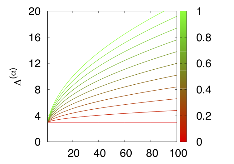
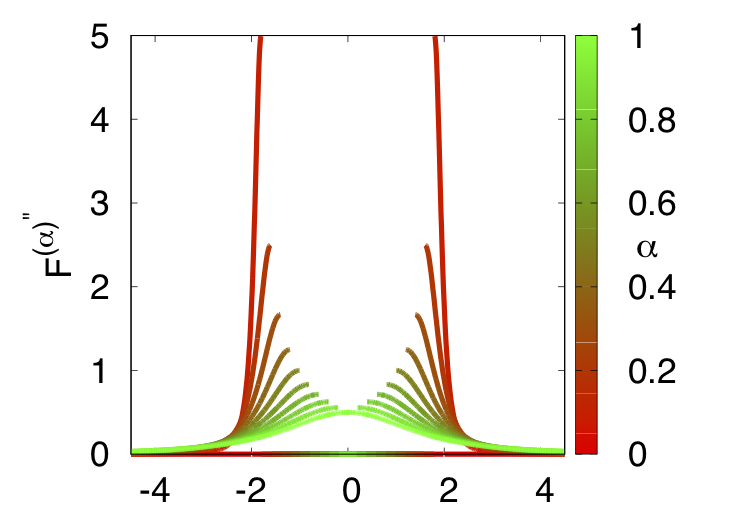
Figure 1: Left: canonical link ψ(α){\psi^{(\alpha)}}, inverse canonical link ψ(α)−1{{\psi^{(\alpha)}}}^{-1} and convex surrogate F(α){F^{(\alpha)}} for the Mα\alpha-loss. Right: plots of Bayes risk L¯(α)​(q){\underline{L}^{(\alpha)}}(q), sensitivity Δ(α)=.ΔL¯(α)​(m)\Delta^{(\alpha)}\stackrel{{\scriptstyle\mathrm{.}}}{{=}}\Delta_{{\underline{L}^{(\alpha)}}}(m), ψ(α)−1​(z){{\psi^{(\alpha)}}}^{-1}(z) and F(α)​(u){F^{(\alpha)}}(u) for the Mα\alpha-loss, for various α\alphas (colors).

In the boosting vs DP picture, there are two extremal losses. The 0/1 loss is the one that necessitates the smallest DP budget (Lemma 5) but achieves the poorest convergence guarantee (Kearns & Mansour 1996, Section 5.1). On the other side of the spectrum, Matsushita loss guarantees the optimal convergence rate (Kearns & Mansour 1996; Nock & Nielsen 2004) but necessitates a considerable DP budget (Lemmata 4, 5). We address the challenge of tuning the convergence rate vs DP budget by creating a new proper symmetric loss, allowing to stand anywhere in between these extremes via a simple tunable parameter α\alpha.

Definition 6

The Mα\alpha-loss is defined for any α∈[0,1]\alpha\in[0,1] by the following partial losses, for y∈{−1,1}y\in\{-1,1\}:

ℓy(α)​(u)\displaystyle\ell^{(\alpha)}_{y}(u) =.\displaystyle\stackrel{{\scriptstyle\mathrm{.}}}{{=}} 2α⋅(1−uu)y/2+2(1−α)⋅⟦yu≤y/2⟧.\displaystyle 2\alpha\cdot\left(\frac{1-u}{u}\right)^{\nicefrac{{y}}{{2}}}+2(1-\alpha)\cdot\llbracket yu\leq y/2\rrbracket.

It is easy to check that the Mα\alpha-loss is proper (strictly if α>0\alpha>0) and symmetric, as well as its Bayes risk is a convex combination of those of the 0/1 and Matsushita losses:

L¯(α)​(u)\displaystyle{\underline{L}^{(\alpha)}}(u) =\displaystyle= α⋅L¯Mat​(u)+(1−α)⋅L¯0/1​(u).\displaystyle\alpha\cdot{\underline{L}^{\mbox{{\tiny Mat}}}}(u)+(1-\alpha)\cdot{\underline{L}^{\mbox{\tiny{{0/1}}}}}(u).

It is also not hard to show that the sensitivity intrapolates between both losses’ sensitivities using Lemma 5.

Corollary 7

The sensitivity (7) of the Mα\alpha-loss satisfies ΔL¯(α)≤ΔL¯(α)∗​(m)=.3+2​α​(m−1)\Delta_{{\underline{L}^{(\alpha)}}}\leq\Delta^{*}_{{\underline{L}^{(\alpha)}}}(m)\stackrel{{\scriptstyle\mathrm{.}}}{{=}}3+2\alpha(\sqrt{m}-1).

Because of the 0/1 loss is not differentiable, getting the inverse canonical link and the convex surrogate is trickier.

Theorem 8

The canonical link ψ(α){\psi^{(\alpha)}}, inverse canonical link ψ(α)−1{{\psi^{(\alpha)}}}^{-1} and surrogate F(α){F^{(\alpha)}} of the Mα\alpha-loss are as in Fig. 1.

5 Boosting with the Mα\alpha-loss

⊳\triangleright Boosting decision trees: We know from the last Section that the Mα\alpha-loss allows, by tuning α\alpha, to continuously change the sensitivity of the criterion between the minimal (α=0\alpha=0) and a maximal one (α=1\alpha=1). We are now going to show that the criterion allows as well to intrapolate between optimal boosting regime (α=1\alpha=1) and a "minimal" convergence guarantee (α=0\alpha=0), thereby completing the boosting vs privacy picture for the Mα\alpha-loss. We first tackle the induction of a single DT as in Kearns & Mansour 1996. Boosting start by formulating a Weak Learning Assumption (WLA) which gives a weak form of correlation with labels for the elementary block of a classifier. In the case of a DT, such a block is a split. So, consider leaf λ\lambda and a test g:𝒳→{0,1}g:{\mathcal{X}}\rightarrow\{0,1\} that splits the leaf in two, the examples going to the left (for which g=0g=0) and those going to the right (for which g=1g=1). The relative weight of positive examples reaching λ\lambda is q∈(0,1)q\in(0,1), where q≠0,1q\neq 0,1 ensures that the leaf is not pure. Define the balanced weights at leaf λ\lambda to be (a) w~i=0\tilde{w}_{i}=0 if 𝒙i∉λ\bm{x}_{i}\not\in\lambda, else (b) w~i=1/(2​q)\tilde{w}_{i}=1/(2q) if yi=+1y_{i}=+1, else (c) w~i=1/(2​(1−q))\tilde{w}_{i}=1/(2(1-q)). Let 𝒘~λ\tilde{\bm{w}}_{\lambda} denote the complete distribution and g+/−∈{−1,1}𝒳g^{\nicefrac{{+}}{{-}}}\in\{-1,1\}^{\mathcal{X}} as g+/−=.−1+2​gg^{\nicefrac{{+}}{{-}}}\stackrel{{\scriptstyle\mathrm{.}}}{{=}}-1+2g. We adopt the edge notation η⁡(𝒘~,h)=.∑iw~i​yi​h​(𝒙i)\eta(\tilde{\bm{w}},h)\stackrel{{\scriptstyle\mathrm{.}}}{{=}}\sum_{i}\tilde{w}_{i}y_{i}h(\bm{x}_{i}) for any h∈ℝ𝒳h\in\mathbb{R}^{\mathcal{X}}. Suppose γ>0\upgamma>0 a constant.

Definition 9

(WLA for DT) Split gg at leaf λ\lambda satisfies the γ\upgamma-WLA iff |η⁡(𝐰~λ,g+/−)|≥γ|\eta(\tilde{\bm{w}}_{\lambda},g^{\nicefrac{{+}}{{-}}})|\geq\upgamma.

Definition 9 is not the same as Kearns & Mansour 1996, but it is equivalent (App., §\lx@sectionsign 14) and in fact more convenient for our framework. A random split would not satisfy the WLA so the WLA enforces the existence of splits at least moderately correlated with the class. Top-down DT induction usually does not proceed by optimizing the split based on the WLA, but in fact it can be shown that the WLA implies good splits according to top-down DT induction criteria Kearns & Mansour 1996. So we let hℓh_{\ell} denote the current DT with ℓ\ell leaves and ℓ−1\ell-1 internal nodes. We grow it to get hℓ+1h_{\ell+1} by minimizing L¯(αℓ){\underline{L}^{(\alpha_{\ell})}} as:

L¯(αℓ)​(hℓ+1)\displaystyle{\underline{L}^{(\alpha_{\ell})}}(h_{\ell+1}) =.\displaystyle\stackrel{{\scriptstyle\mathrm{.}}}{{=}} αℓ⋅L¯Mat​(hℓ+1)+(1−αℓ)⋅L¯err​(hℓ+1),\displaystyle\alpha_{\ell}\cdot{\underline{L}^{\mbox{{\tiny Mat}}}}(h_{\ell+1})+(1-\alpha_{\ell})\cdot{\underline{L}^{\mbox{{\tiny err}}}}(h_{\ell+1}),

where hℓ+1h_{\ell+1} is hℓh_{\ell} with a leaf λ∈Λ⁡(hℓ)\lambda\in\Lambda(h_{\ell}) replaced by a split. Noting K≥0K\geq 0 a constant, w=.∑iwiw\stackrel{{\scriptstyle\mathrm{.}}}{{=}}\sum_{i}w_{i} and

w~ℓ\displaystyle\tilde{w}_{\ell} =.\displaystyle\stackrel{{\scriptstyle\mathrm{.}}}{{=}} (1w)⋅∑iwi⟦i∈λℓ⟧∈[0,1]\displaystyle\left(\frac{1}{w}\right)\cdot\sum_{i}w_{i}\llbracket i\in\lambda_{\ell}\rrbracket\quad\in[0,1] (11)

the total normalized weight of the examples reaching λℓ\lambda_{\ell}, we say that the sequence of α\alphas is KK-monotonic iff αℓ≤αℓ−1⋅exp⁡(K​w~ℓ​(1−αℓ−1))\alpha_{\ell}\leq\alpha_{\ell-1}\cdot\exp\left(K\tilde{w}_{\ell}(1-\alpha_{\ell-1})\right) for any ℓ>2\ell>2 (and α1∈[0,1]\alpha_{1}\in[0,1]). Since the parameter in the exp\exp is ≥0\geq 0, KK-monotonicity prevents the sequence from growing too fast.

Theorem 10

Suppose all splits satisfy the γ\upgamma-WLA and the sequence of α\alphas is (γ2/16)(\upgamma^{2}/16)-monotonic. Then ∀ξ∈(0,1]\forall\xi\in(0,1], the empirical risk of hLh_{L} satisfies ε0/1​(hL)≤ξ\varepsilon_{\mbox{\tiny{0/1}}}(h_{L})\leq\xi as long as

∑ℓ=1Lw~ℓ​αℓ\displaystyle\sum_{\ell=1}^{L}\tilde{w}_{\ell}\alpha_{\ell} ≥\displaystyle\geq (16γ2)⋅log⁡(1ξ).\displaystyle\left(\frac{16}{\upgamma^{2}}\right)\cdot\log\left(\frac{1}{\xi}\right). (12)

It is worth remarking that this is indeed a generalization of Kearns & Mansour 1996: suppose αℓ=α\alpha_{\ell}=\alpha constant (which is (γ2/16)(\upgamma^{2}/16)-monotonic ∀γ≥0\forall\upgamma\geq 0) and we pick at each iteration the heaviest leaf to split. We thus have w~ℓ≥1/ℓ\tilde{w}_{\ell}\geq 1/\ell, assuming further it satisfies the WLA. Since ∑ℓ=1L(1/ℓ)≥∫1L+1𝑑z/z=log⁡(L+1)\sum_{\ell=1}^{L}(1/\ell)\geq\int_{1}^{L+1}\mathrm{d}z/z=\log(L+1), (12) is guaranteed if

L\displaystyle L ≥\displaystyle\geq (1ξ)16α​γ2,\displaystyle\left(\frac{1}{\xi}\right)^{\frac{16}{\alpha\upgamma^{2}}}, (13)

which, for α=1\alpha=1, is in fact the square root of the bound in Kearns & Mansour 1996 and is thus significantly better. Rather than a quantitative improvement, we were seeking for a qualitative one as Kearns & Mansour 1996 pick the heaviest leaf to split, which means using DP budget to find it. To see how we can get essentially the same guarantee without this contraint, suppose instead that we split all current leaves, all of them satisfying the WLA33 3 This happens to be reasonable on domains big enough, for small trees or when the set from which gg is picked is rich enough.. Since ∑λw~​(λ)=1\sum_{\lambda}\tilde{w}(\lambda)=1 (those weights are normalized), once we remark that it takes one split for the root, then two, then four and so on to fully split the current leaves, LL boosting iterations guarantee a full split up to depth O⁡(log⁡(L))O(\log(L)), which delivers the same condition as (13) with an eventual change in the exponent constant. Our result is also a generalization of Kearns & Mansour 1996 since it allows to tune α\alpha during learning, which is important for us (§\lx@sectionsign 6).

⊳\triangleright Boosting linear combinations of classifiers: we now consider that we build a Linear Combination (LC) of classifiers, HT=.∑t=1Tβt​htH_{T}\stackrel{{\scriptstyle\mathrm{.}}}{{=}}\sum_{t=1}^{T}\beta_{t}h_{t}, where ht:𝒳→ℝh_{t}:\mathcal{X}\rightarrow\mathbb{R} is a real valued classifier — this could be a DT or any other applicable classifier. We tackle the problem of achieving boosting-compliant convergence when building HTH_{T}, which means we have a WLA on each hth_{t}. We also assume ∃M>0\exists M>0 such that |ht|≤M|h_{t}|\leq M. Let 𝒘t∈[0,1]m\bm{w}_{t}\in[0,1]^{m} an unnormalized weight vector on 𝒮\mathcal{S}, tt denoting the iteration number from which hth_{t} is obtained. Noting w~t=.(1/m)⋅∑iwt​i∈[0,1]\tilde{w}_{t}\stackrel{{\scriptstyle\mathrm{.}}}{{=}}\left(\nicefrac{{1}}{{m}}\right)\cdot\sum_{i}w_{ti}\in[0,1] the expected unnormalized weight at iteration tt, we also let 𝒘~t=.(1/(m​w~t))⋅𝒘t\tilde{\bm{w}}_{t}\stackrel{{\scriptstyle\mathrm{.}}}{{=}}(1/(m\tilde{w}_{t}))\cdot\bm{w}_{t} denote the normalized weight vector at iteration tt. The WLA is as follows.

Definition 11

(WLA for LC) hth_{t} obtained at iteration tt satisfies the γ\upgamma-WLA iff |η⁡(𝐰~t,ht)|≥γ​M|\eta(\tilde{\bm{w}}_{t},h_{t})|\geq\upgamma M.

Remark that this definition is similar to Definition 9, since |g+/−|=1|g^{\nicefrac{{+}}{{-}}}|=1. All the crux is now how to get the weight vectors 𝒘t\bm{w}_{t} so that we can prove a boosting-compliant convergence rate using the Mα\alpha-loss. We do so using a standard mechanism, which consists in initializing 𝒘1=.(1/2)⋅𝟏\bm{w}_{1}\stackrel{{\scriptstyle\mathrm{.}}}{{=}}(1/2)\cdot\bm{1} (unnormalized) and then using the mirror update of the Mα\alpha-loss to update weights after hth_{t} has been received:

w(t+1)​i\displaystyle w_{(t+1)i}\hskip-8.5359pt ←\displaystyle\leftarrow ψ(α)−1​(−βt​yi​ht​(𝒙i)+ψ(α)​(wt​i)),\displaystyle\hskip-8.5359pt{{\psi^{(\alpha)}}}^{-1}\left(-\beta_{t}y_{i}h_{t}(\bm{x}_{i})+{{\psi^{(\alpha)}}}(w_{ti})\right), (14)

where βt\beta_{t} is a leveraging coefficient for hth_{t} in the final classifier, taken to be βt←a​w~t⋅η⁡(𝒘~t,ht)\beta_{t}\leftarrow a\tilde{w}_{t}\cdot\eta(\tilde{\bm{w}}_{t},h_{t}), where aa is a constant chosen beforehand anywhere in interval (α/M2)⋅[1−π,1+π](\alpha/M^{2})\cdot\left[1-\pi,1+\pi\right], π∈[0,1)\pi\in[0,1) quantifying the freedom in choosing aa. This is sufficient to complete the description of the algorithm (also given in extenso in App., §\lx@sectionsign 15).

Theorem 12

Suppose all hth_{t} satisfy the γ\upgamma-WLA. Then ∀ξ∈[0,1]\forall\xi\in[0,1], we have ε0/1​(HT)≤ξ\varepsilon_{\mbox{\tiny{0/1}}}(H_{T})\leq\xi as long as:

∑t=1Tw~t2\displaystyle\sum_{t=1}^{T}\tilde{w}^{2}_{t} ≥\displaystyle\geq 2​(1−ξ)(1−π2)​γ2​α.\displaystyle\frac{2(1-\xi)}{(1-\pi^{2})\upgamma^{2}\alpha}. (15)

This Theorem has a very similar flavour on boosting conditions as we had in Theorem 10 for DTs but its dependence on ξ\xi is comparatively misleading. What Theorem 12 indeed tells us is boosting for LC is efficient under the WLA as long as wtw_{t} is "large" enough in [0,1][0,1]. The weight update in (14) meets the classical boosting property that an example has its weight directly correlated to classification: the better, the smaller its weight (Cf the plot of ψ(α)−1{{\psi^{(\alpha)}}}^{-1} in Figure 1). Hence, as classification gets better, the sum on the LHS of (15) increases at smaller rate and if ξ\xi is too small, this means a potentially larger number of iterations to meet (15).

6 Privacy and boosting: objective calibration

We have so far described the complete picture of DP for DT with any noisification mechanism that relies on the sensitivity of a Bayes risk, and the complete but noise-free boosting picture for the Mα\alpha-loss for DT and LC. We now assemble them. In an iterative boosted combination of DT, two locations of privacy budget spending can make the full classifier meet DP: (a) node splitting in trees, (b) leaf predictions in trees. The protection of the leveraging coefficients βt\beta_{t} can be obtained in two ways: either we multiply each leaf prediction by βt\beta_{t}, then replace βt←1\beta_{t}\leftarrow 1 and then carry out (b), or use the faster but more conservative approach to just do (b) e.g. with the Laplace mechanism from which follows the protection of βt\beta_{t} (§\lx@sectionsign 5). We do not carry out pruning as boosting alone can be sufficient for good generalization, see e.g. Schapire et al. 1998, Bartlett & Mendelson 2002, and pruning also requires privacy budget (Fletcher & Islam 2019, §\lx@sectionsign 3.5). The public information is the attribute domain, which is standard (Fletcher & Islam 2019), and we consider that each continuous attributes is regularly quantized using a public number vqv_{q} of values. This makes sense for many common attributes like age, percentages, $\$-value, and this can contribute to ease interpretation; this also has three technical justifications: (1) a private approaches requires budget, (2) vqv_{q} allows to tightly control the computational complexity of the whole DT induction, (3) boosting does not require exhaustive split search provided vqv_{q} is not too small (more in App., §\lx@sectionsign17.1).

⊳\triangleright Private induction of a DT: objective calibration. The overall privacy budget ε\varepsilon is split in two proportions: βtree\beta_{\mbox{{\tiny tree}}} for node splitting (a) and βpred=.1−βtree\beta_{\mbox{{\tiny pred}}}\stackrel{{\scriptstyle\mathrm{.}}}{{=}}1-\beta_{\mbox{{\tiny tree}}} leaves’ predictions (b). The basis of our approach to split nodes is the nice — but never formally analyzed — trick of Friedman & Schuster 2010 which consists in using the exponential mechanism to choose splits. Let 𝒢\mathcal{G} denote the whole set of splits. The probability to pick g∈𝒢g\in\mathcal{G} to split leaf λ∈Λ⁡(hℓ)\lambda\in\Lambda(h_{\ell}) is:

pexp​((,,,))\displaystyle p_{\mbox{\tiny{{exp}}}}((g,\lambda))\hskip-8.5359pt ∝\displaystyle\propto exp⁡(−ε⁡(hℓ,λ)​w​(𝒮)​F​(hℓ⊕(g,λ))2​ΔL¯(α)∗​(m)),\displaystyle\hskip-8.5359pt\exp\left(-\frac{\varepsilon(h_{\ell},\lambda)w(\mathcal{S})F(h_{\ell}\oplus(g,\lambda))}{2\Delta^{*}_{{\underline{L}^{(\alpha)}}}(m)}\right), (16)

where notation hℓ⊕(g,λ)h_{\ell}\oplus(g,\lambda) refers to decision tree hℓh_{\ell} in which leaf λ\lambda is replaced by split gg, w⁡(𝒮)⋅F⁡(hℓ⊕(g,λ))w(\mathcal{S})\cdot F(h_{\ell}\oplus(g,\lambda)) is the unnormalized Bayes risk (Section 3) and ΔL¯(α)∗​(m)\Delta^{*}_{{\underline{L}^{(\alpha)}}}(m) is given in Lemma 7. ε⁡(hℓ,λ)\varepsilon(h_{\ell},\lambda) is the fraction of the total privacy budget allocated to the split. So far, all recorded approaches consider uniform budget spending (Fletcher & Islam 2019) but such a strategy is clearly oblivious to the accuracy vs privacy dilemma as explained in Section 3. We now introduce a more sophisticated approach exploiting our result, allowing to bring strong probabilistic guarantees on boosting while being private. The intuition behind is simple: the "support" (total unnormalized weight) of a node is monotonic decreasing on any root-to-leaf path. Therefore, we should typically increase the budget spent in low-depth splits because (i) it impacts more examples and (ii) it increases the likelihood of picking the splits that meet the WLA in the exponential mechanism (16). Consequently, we also should pick α\alpha larger for low-depth splits, to increase the early boosting rate and drive as fast as possible the empirical risk to the minimum, yet monitoring the dependency of the exponential mechanism in α\alpha to control the probability of picking the splits that meet the WLA. This may look like a quite intricate set of dependences between privacy and boosting, but here is a solution that matches all of them. If we denote h1h_{1} the tree reduced to a leaf from which hℓh_{\ell} was built, 0pt(.)0pt(.) as the depth of a node, dd the maximal depth of a tree and TT the number of trees in the combination, then we let:

αℓ\displaystyle\alpha_{\ell} =.\displaystyle\stackrel{{\scriptstyle\mathrm{.}}}{{=}} ε0/1​(hℓ)ε0/1​(h1)(∈[0,1]),\displaystyle\frac{\varepsilon_{\mbox{\tiny{0/1}}}(h_{\ell})}{\varepsilon_{\mbox{\tiny{0/1}}}(h_{1})}\quad(\in[0,1]), (17)
ε⁡(hℓ,λ)\displaystyle\varepsilon(h_{\ell},\lambda) =\displaystyle= βtreeT​d​20​p​t​(λ)⋅ε.\displaystyle\frac{\beta_{\mbox{{\tiny tree}}}}{Td2^{0pt(\lambda)}}\cdot\varepsilon. (18)

The choice of αℓ\alpha_{\ell} makes it decreasing along every path from the root: while we split the root using Matsushita loss (α=1\alpha=1), which guarantees optimal boosting rate, we gradually move in deeper leaves to using more of the Bayes risk of the 0/1 loss, which may reduce the rate but reduces privacy budget used as well. Referring to objective perturbation which noisifies the loss (Chaudhuri et al. 2011), we call our method that tunes the loss objective calibration (O.C).

We formally analyze O.C. First, remark that the total budget spent for one tree is βtree​ε/T\beta_{\mbox{{\tiny tree}}}\varepsilon/T, which fits in the global budget ε\varepsilon. To develop the boosting picture, we build on the γ\upgamma-WLA. We first remark that for any hh, leaf λ∈Λ⁡(h)\lambda\in\Lambda(h) and split g∈𝒢g\in\mathcal{G}, there exists u≥0u\geq 0 such that

L¯(α)​(h)−L¯(α)​(h⊕(g,λ))\displaystyle\hskip-8.5359pt{\underline{L}^{(\alpha)}}(h)-{\underline{L}^{(\alpha)}}(h\oplus(g,\lambda))\hskip-8.5359pt =\displaystyle= u⋅γ2​α​w~​(λ)16⋅L¯(α)​(h).\displaystyle\hskip-8.5359ptu\cdot\frac{\upgamma^{2}\alpha\tilde{w}(\lambda)}{16}\cdot{\underline{L}^{(\alpha)}}(h). (19)

This is a simple consequence of the concavity of any Bayes risk. Interestingly, for all splits that satisfy the WLA, it can be shown that we can pick u≥1u\geq 1 (App., §\lx@sectionsign 16). Let us denote 𝒢wla⊆𝒢\mathcal{G}_{\mbox{\tiny{{wla}}}}\subseteq\mathcal{G} the whole set of such boosting amenable splits, and let 𝒢lazy=.𝒢\𝒢wla\mathcal{G}_{\mbox{\tiny{{lazy}}}}\stackrel{{\scriptstyle\mathrm{.}}}{{=}}\mathcal{G}\backslash\mathcal{G}_{\mbox{\tiny{{wla}}}} denote the remaining splits. The exponential mechanism might of course pick splits in 𝒢lazy\mathcal{G}_{\mbox{\tiny{{lazy}}}} but let us assume that there is at least a small "gap" between those splits and those of 𝒢wla\mathcal{G}_{\mbox{\tiny{{wla}}}}, in such a way that for any split in 𝒢lazy\mathcal{G}_{\mbox{\tiny{{lazy}}}}, (19) holds only for u≤δu\leq\delta for some δ<1\delta<1. This property always holds for some δ<1\delta<1 but let us assume that this δ\delta is a constant, just like the γ\upgamma of the WLA, and call it the δ\delta-Gap assumption. Let 𝒩⁡(h){\mathcal{N}}(h) denotes the set of nodes of hh, including leaves in Λ⁡(h)\Lambda(h). The tree-efficiency of ν∈𝒩⁡(h)\nu\in{\mathcal{N}}(h) in hh is defined as

J⁡(ν,h)\displaystyle J(\nu,h) =.\displaystyle\stackrel{{\scriptstyle\mathrm{.}}}{{=}} 8​w~​(ν)​ε0/1​(h)220​p​t​(ν)∈[0,1],\displaystyle\frac{8\tilde{w}(\nu)\varepsilon_{\mbox{\tiny{0/1}}}(h)^{2}}{2^{0pt(\nu)}}\quad\in[0,1], (20)

where w~​(ν)\tilde{w}(\nu) is the normalized weights of examples reaching ν\nu. Let ℒ\mathcal{L} be a subset of indexes of the leaves split from h1h_{1} to create a depth-dd tree, with unnormalized weights 𝒘\bm{w}. Each element ℓ\ell refers to a couple (λℓ,hℓ)(\lambda_{\ell},h_{\ell}) where hℓh_{\ell} is the tree in which λℓ\lambda_{\ell} was replaced by a split.

Theorem 13

Suppose the exponential mechanism is implemented with αℓ\alpha_{\ell} and εℓ\varepsilon_{\ell} as in (17), (18). Suppose T​d≤log⁡mTd\leq\log m, m≥3m\geq 3 and both the γ\upgamma-WLA and δ\delta-Gap assumptions hold. Suppose that ∀ℓ∈ℒ\forall\ell\in\mathcal{L},

|𝒢wlaℓ|\displaystyle|{\mathcal{G}_{\mbox{\tiny{{wla}}}}}_{\ell}| ≥\displaystyle\geq |𝒢lazyℓ|⋅exp⁡(−Ω⁡(J⁡(λℓ,hℓ)⋅ε​mlog⁡m)).\displaystyle|{\mathcal{G}_{\mbox{\tiny{{lazy}}}}}_{\ell}|\cdot\exp\left(-\Omega\left(J(\lambda_{\ell},h_{\ell})\cdot\frac{\varepsilon\sqrt{m}}{\log m}\right)\right).

Then, for any ξ>0\xi>0, if

minℓ∈ℒ⁡J⁡(λℓ,hℓ)\displaystyle\min_{\ell\in\mathcal{L}}J(\lambda_{\ell},h_{\ell}) =\displaystyle= Ω⁡(log⁡mε​m​log⁡|ℒ|ξ),\displaystyle\Omega\left(\frac{\log m}{\varepsilon\sqrt{m}}\log\frac{|\mathcal{L}|}{\xi}\right), (21)

then with probability ≥1−ξ\geq 1-\xi, all splits chosen by the exponential mechanism to split the leaves indexed in ℒ\mathcal{L} satisfy the WLA.

The proof (App., §\lx@sectionsign 16), explicits all hidden constants. We insist on the message that Theorem 13 carries about the exponential mechanism: under the WLA/Gap assumptions and a size constraint on each 𝒢wlat{\mathcal{G}_{\mbox{\tiny{{wla}}}}}_{t} (which by the way authorises it to be reasonably smaller than 𝒢lazyt{\mathcal{G}_{\mbox{\tiny{{lazy}}}}}_{t}), the exponential mechanism has essentially no negative impact on boosting with high probability. This, we believe, is a very strong incentive in favor of the exponential mechanism as designed in Friedman & Schuster 2010. Finally, the condition T​d≤log⁡mTd\leq\log m could be replaced by a low-degree polylog but even without doing so, it actually fits well in a series of experimental work (Fletcher & Islam 2019), for example Mohammed et al. 2015 (T​d=4Td=4), Friedman & Schuster 2010 (T​d=5Td=5), Fletcher & Islam 2015 (T​d=20Td=20).

Remark 14

Theorem 13 reveals another reason why we should indeed put emphasis on boosting on low-depth nodes: for any node of hh, if its tree efficiency is above a threshold, then so is the case for all nodes along a shortest path from this node to the root of hh. Hence the largest set ℒ\mathcal{L} for which (21) holds corresponds to a subtree of hh with the same root.

To get a simple idea of how (21) vanishes with mm, remark that |ℒ|≤2d+1−1|\mathcal{L}|\leq 2^{d+1}-1. Condition (207) is therefore satisfied if for example ε,ξ,d\varepsilon,\xi,d are related to mm as

log⁡(m)m\displaystyle\frac{\log(m)}{\sqrt{m}} =\displaystyle= o⁡(ε),\displaystyle o(\varepsilon),
d,log⁡1/ξ\displaystyle d,\log\nicefrac{{1}}{{\xi}} =\displaystyle= o⁡(mlog⁡m),\displaystyle o\left(\frac{\sqrt{m}}{\log m}\right),

and in this case the constraint on minℓ∈ℒ⁡J⁡(λℓ,h)\min_{\ell\in\mathcal{L}}J(\lambda_{\ell},h) in (208) vanishes with mm. This makes that strong privacy regimes can fit to Theorem 13, e.g. with ε=log1+c⁡(m)/m\varepsilon=\log^{1+c}(m)/\sqrt{m} for c>0c>0 a constant.

⊳\triangleright Private predictions at the leaves: because our trees output real values, we use the Laplace mechanism. This fits well with the WLA using |ht|≤M|h_{t}|\leq M (Definition 11), for the sensitivity of the mechanism (Dwork & Roth 2014).

7 Experiments

ε\varepsilon 0.010.01 0.10.1 11 1010 2525
(O.C, 0.1, 1.0) (14,3,5) (13,2,6) (9,3,9) (5,4,11) (8,6,6)
Table 1: Summary, on the 19 domains, of the #\# of domains for which one strategy for α\alpha in {\{objective calibration (O.C), 0.10.1, 1,01,0}\} leads to the best result (ties lead to sums >19>19).
perf. wrt α\alphas, w/o DP perf. wrt α\alphas, with DP     #\#leaves, w/o DP #\#leaves, with DP
Refer to caption Refer to caption     Refer to caption
Figure 2: UCI domain banknote: in each plot, xx depicts test errors and yy a cumulated %\% of runs of bdpeα having test error at most xx. In each pane (left, right), the left plot is without DP and the right plot is with DP. Left pane: comparison of bdpeα for three strategies on α\alpha (see text). Right pane: mean ±\pm stddev for the number of leaves in the related trees (see text).

We have performed 10-folds stratified CV experiments on 19 UCI domains, detailed in App., Section 17.3, ranging from m⋅n<m\cdot n< 3 000 to m⋅n>m\cdot n> 200 000 . We have compared our approach, bdpeα, to two state of the art implementation of RFs based on Fletcher & Islam 2017 but replacing the smooth sensitivity by the global sensitivity (Definition 1). RFs have the appealing property for DP that privacy budget needs only be spent at the leaves: we have tried both the Laplace (RF-L) and the exponential (RF-E) mechanisms (see App., §\lx@sectionsign 17.2) with RFs containing T=21T=21 trees to prevent ties. We have performed three kinds of experiments: (i) check that bdpeα performs well and complies with the boosting theory in the privacy-free case, (ii) compare the various flavours of bdpeα in the private case, (iii) compare bdpeα vs RFs in the private case. We ran bdpeα, both private and not private, for all combinations of T∈{2,5,10,20},α∈{0.1,1.0,O.C}T\in\{2,5,10,20\},\alpha\in\{0.1,1.0,\mbox{O.C}\}, depth ∈{1,2,3,4,5,6},ε∈{0.01,0.1,1.0,10.0,25.0},βtree∈{0.1,0.5,0.9}\in\{1,2,3,4,5,6\},\varepsilon\in\{0.01,0.1,1.0,10.0,25.0\},\beta_{\mbox{{\tiny tree}}}\in\{0.1,0.5,0.9\}, and even more parameters (see App., §\lx@sectionsign 17.1), for a total number of boosting experiments alone that far exceeds the million ensemble models learned. When there is no DP constraint, we add in bdpeα the test of whether a leaf is pure – i.e. is not reached by examples of both classes – before attempting to split it (we do not split further pure leaves). When there is DP however, we do not make the test in order not to spend privacy budget, and so bdpeα  builds trees in which all leaves are at the required depth. The App., §\lx@sectionsign 17, gives the experiments in greater details, summarized here.
⊳\triangleright bdpeα, with and without noise: Figure 2, left pane, displays a picture that can be observed more or less over all domains: bdpeα with α=1\alpha=1 tends to obtain better results than with α=0.1\alpha=0.1, which complies with Theorems 10 and 12, and with the boosting theory more generally (Kearns & Mansour 1996). Three additional observations emerge: (a) objective calibration (O.C) is competitive without noise, (b) this also holds with noise, which we believe indicate a good compromise between convergence rates and safekeeping privacy budget in bdpeα  (Section 3) and contributes to experimentally validate our theory in Section 6; (c) DP curves display predictable degradations due to noise, but on many domains noisification still gives interesting results compared to the noise-free setting: in banknote for example (Figure 2), more than 2/3 of the private runs with O.C get test error ≤20%\leq 20\%, an upperbound test error for noise-free boosting.
⊳\triangleright bdpeα in various privacy regimes: Table 1 is an extremal experiments which looks at the best models that can be learned under DP under various ε\varepsilon. The picture that seems to emerge is that objective calibration is the best technique for high privacy demand, which we take as a good sign given our theory (Section 6). Obviously, the experiments aggregate a number of parameters for each ε\varepsilon, such as T,d,βtreeT,d,\beta_{\mbox{{\tiny tree}}}, so to really get the best of a regime for α\alpha, one should be able to have clues on how to fix those other parameters. It turns out that the experiments display that this should be possible. In particular, for each domain, the value βtree\beta_{\mbox{{\tiny tree}}} does not seem to significantly matter to get the best results but the model size parameters seem to matter a lot more: for each domain, there is a particular regime of d,Td,T that tends to give the top DP results (like rather deep trees for banknote, Figure 2). App., Section Summary in d,Td,T for the best DP in bdpeα presents the whole list details. This, we believe, is important, in particular for domains where TT is small like page, as some RFs approaches fit huge sets reducing interpretability (Fletcher & Islam 2019, Table I).
⊳\triangleright bdpeα vs (RF-L and RF-E): a Table (4, given in App., S§\lx@sectionsign Summary of the comparison bdpeα vs RFs with DP) computes over all 19 domains the %\% of runs where bdpeα beats RFs, among all runs for which one approach statistically significantly (pval<0.01p_{\mbox{\tiny val}}<0.01) beats the other. The scale heavily tips in favor of bdpeα when it boosts T=20T=20 trees: O.C and α=1.0\alpha=1.0 are significantly superior than RF-E and RF-L on more than 80 %\% of such cases (less than 4%\% of the differences are not significant). This means two things: first, for these strategies of bdpeα, there is not much care needed to optimize some parameters of bdpeα (d,βpredd,\beta_{\mbox{{\tiny pred}}}) to get to or beat SOTA, which is good news; second, this suggests that we can compete with RFs on much smaller trees, which is indeed displayed in the left pane of Table 4 where bdpeα fits less than ten times trees than RFs, and still beat those in a majority of cases, which is good news for interpretability. When we drill down into the results as a function of ε\varepsilon, we observe that bdpeα tends to be especially good against RFs for high privacy regimes (e.g.ε=0.01\varepsilon=0.01).
⊳\triangleright bdpeα in the vq=10v_{q}=10 vs vq=50v_{q}=50 regime: the previous summarizes experiments for a regular quantization with vq=10v_{q}=10 of the continuous attributes. Our experiments (App., Section Summary comparison vq=10v_{q}=10 vs vq=50v_{q}=50 (M=10M=10)) also contain a summary of the comparisons for bdpeα when we rather use vq=50v_{q}=50. Notice that multiplying by five the potential number of splits significantly affects the time complexity of the algorithm. The results display that the impact varies as a function of the domain at hand. There can be significant improvements: qsar and winewhite are two domains for which vq=50v_{q}=50 buys more than 2%\% improvement for objective calibration, a clear winner among all tested strategies for α\alpha. On banknote, the improvement is more in favor of α=1.0\alpha=1.0. On winered, there is no significant improvement for the best strategy and apart from a seemingly better "concentration" of more than 3/4 of the runs of objective calibration towards its best results with vq=50v_{q}=50, there is no apparent gain otherwise.

8 Conclusion

While boosted ensemble of DTs have long shown their accuracy in international competitions, to our knowledge nothing is known on how to fit them in a differentially private framework while keeping some of the boosting guarantees, a setting in which random forests have been reigning supreme. In this paper, we first establish the existence of a nontrivial tradeoff to push boosting methods in a differentially private framework. To address this tradeoff, we first create a tunable proper canonical loss, whose boosting rate and sensitivity can be controlled up to optimal boosting rate, or minimal sensitivity. We then show guaranteed boosting rates for both the induction of DTs and ensembles using this loss, of independent interest. We introduce objective calibration as a way to dynamically tune this loss and make the most of boosting under a given privacy budget with high probability. Experiments reveal that our approach manages to significantly beat random forests, that the best private models tend to be learned by objective calibration, and that our technique appears all the better on high privacy regimes.

Acknowledgments

The authors thank Sam Fletcher and Borja Balle for comments on this material.

References

  • Agarwal et al. (2019) Agarwal, A., Dudík, M., and Wu, Z.-S. Fair regression: Quantitative definitions and reduction-based algorithms. In 36th ICML, pp. 120–129, 2019.
  • Alistarh et al. (2017) Alistarh, D., Grubic, D., Li, J., Tomioka, R., and Vojnovic, M. QSGD: communication-efficient SGD via gradient quantization and encoding. In NIPS*30, pp. 1707–1718, 2017.
  • Andriushchenko & Hein (2019) Andriushchenko, M. and Hein, M. Provably robust boosted decision stumps and trees against adversarial attacks. In NeurIPS*32 and NeurIPS’19 workshop on Machine Learning with Guarantees, 2019. URL https://www.idiap.ch/workshop/smld2019/slides/smld2019_maksym_andriushchenko.pdf.
  • Bartlett & Mendelson (2002) Bartlett, P.-L. and Mendelson, S. Rademacher and gaussian complexities: Risk bounds and structural results. JMLR, 3:463–482, 2002.
  • Boyd & Vandenberghe (2004) Boyd, S. and Vandenberghe, L. Convex optimization. Cambridge University Press, 2004.
  • Breiman (1996) Breiman, L. Bagging predictors. MLJ, 24:123–140, 1996.
  • Breiman et al. (1984) Breiman, L., Freidman, J. H., Olshen, R. A., and Stone, C. J. Classification and regression trees. Wadsworth, 1984.
  • Buja et al. (2005) Buja, A., Stuetzle, W., and Shen, Y. Loss functions for binary class probability estimation and classification: structure and applications, 2005. Technical Report, University of Pennsylvania.
  • Chaudhuri et al. (2011) Chaudhuri, K., Monteleoni, C., and Sarwate, A.-D. Differentially private empirical risk minimization. JMLR, 12:1069–1109, 2011.
  • Chen & Guestrin (2016) Chen, T. and Guestrin, C. XGBoost: A scalable tree boosting system. In 22nd KDD, pp. 785–794, 2016.
  • Drumond et al. (2018) Drumond, M., Lin, T., Jaggi, M., and Falsafi, B. Training DNNs with hybrid block floating point. In NeurIPS*31, pp. 451–461, 2018.
  • Dua & Graff (2017) Dua, D. and Graff, C. UCI machine learning repository, 2017. URL http://archive.ics.uci.edu/ml.
  • Dwork & Roth (2014) Dwork, C. and Roth, A. The algorithmic foudations of differential privacy. Found. &\& Trends in TCS, 9:211–407, 2014.
  • Dwork et al. (2006) Dwork, C., McSherry, F., Nissim, K., and Smith, A. Calibrating noise to sensitivity in private data analysis. In 3rd TCC, pp. 265–284, 2006.
  • Fan et al. (2003) Fan, W., Wang, H., Yu, P.-S., and Ma, S. Is random model better? on its accuracy and efficiency. In ICDM’03, 2003.
  • Fletcher & Islam (2015) Fletcher, S. and Islam, M.-Z. A differentially private decision forest. In AusDM’15, pp. 99–108, 2015.
  • Fletcher & Islam (2017) Fletcher, S. and Islam, M.-Z. Differentially private random decision forests using smooth sensitivity. Expert Systems with Applications, 78:16 – 31, 2017.
  • Fletcher & Islam (2019) Fletcher, S. and Islam, M.-Z. Decision tree classification with differential privacy: A survey. ACM Computing Surveys, 2019.
  • Friedman & Schuster (2010) Friedman, A. and Schuster, A. Data mining with differential privacy. In Proc. of the 16th ACM KDD, pp. 493–502, 2010.
  • Friedman et al. (2000) Friedman, J., Hastie, T., and Tibshirani, R. Additive Logistic Regression : a Statistical View of Boosting. Ann. of Stat., 28:337–374, 2000.
  • Jacob et al. (2018) Jacob, B., Kligys, S., Chen, B., Zhu, M., Tang, M., Howard, A.-G., Adam, H., and Kalenichenko, D. Quantization and training of neural networks for efficient integer-arithmetic-only inference. In Proc. of the 31st IEEE CVPR, pp. 2704–2713, 2018.
  • Jagielski et al. (2019) Jagielski, M., Kearns, M.-J., Mao, J., Oprea, A., Roth, A., Sharifi-Malvajerdi, S., and Ullman, J. Differentially private fair learning. In 36th ICML, pp. 3000–3008, 2019.
  • Kaplan et al. (2019) Kaplan, H., Mansour, Y., Matias, Y., and Stemmer, U. Differentially private learning of geometric concepts. In 36th ICML, pp. 3233–3241, 2019.
  • Ke et al. (2017) Ke, G., Meng, Q., Finley, T., Wang, T., Chen, W., Ma, W., Ye, Q., and Liu, T.-Y. Lightgbm: A highly efficient gradient boosting decision tree. In NIPS*30, pp. 3146–3154, 2017.
  • Kearns & Mansour (1996) Kearns, M. and Mansour, Y. On the boosting ability of top-down decision tree learning algorithms. In Proc. of the 28th ACM STOC, pp. 459–468, 1996.
  • Maréchal (2005a) Maréchal, P. On a functional operation generating convex functions, part I: duality. J. OTA, 126:175–189, 2005a.
  • Maréchal (2005b) Maréchal, P. On a functional operation generating convex functions, part II: algebraic properties. J. OTA, 126:357–366, 2005b.
  • Masnadi-Shirazi & Vasconcelos (2015) Masnadi-Shirazi, H. and Vasconcelos, N. A view of margin losses as regularizers of probability estimates. JMLR, 16:2751–2795, 2015.
  • McSherry & Talwar (2007) McSherry, F. and Talwar, K. Mechanism design via differential privacy. In 48th IEEE FOCS, pp. 94–103, 2007.
  • Mohammed et al. (2015) Mohammed, N., Barouti, S., Alhadidi, D., and Chen, R. Secure and private management of healthcare databases for data mining. In CBMS’15, pp. 191–196, 2015.
  • Nock & Nielsen (2004) Nock, R. and Nielsen, F. On Domain-Partitioning Induction Criteria: Worst-case Bounds for the Worst-case Based. Theoretical Computer Science, 321:371–382, 2004.
  • Nock & Nielsen (2008) Nock, R. and Nielsen, F. On the efficient minimization of classification-calibrated surrogates. In NIPS*21, pp. 1201–1208, 2008.
  • Nock & Nielsen (2009) Nock, R. and Nielsen, F. Bregman divergences and surrogates for learning. IEEE Trans. PAMI, 31:2048–2059, 2009.
  • Nock & Williamson (2019) Nock, R. and Williamson, R.-C. Lossless or quantized boosting with integer arithmetic. In 36th ICML, pp. 4829–4838, 2019.
  • Quinlan (1993) Quinlan, J. R. C4.5 : programs for machine learning. Morgan Kaufmann, 1993.
  • Reid & Williamson (2010) Reid, M.-D. and Williamson, R.-C. Composite binary losses. JMLR, 11:2387–2422, 2010.
  • Schapire et al. (1998) Schapire, R. E., Freund, Y., Bartlett, P., and Lee, W. S. Boosting the margin : a new explanation for the effectiveness of voting methods. Annals of statistics, 26:1651–1686, 1998.

Appendix

9 Table of contents

Appendix on proofs

 Pg Appendix on Proofs
Proof of Theorem 3

 Pg 10
Proof of Lemma 4

 Pg 11
Proof of Lemma 5

 Pg 12
Proof of Theorem 8

 Pg 13
Proof of Theorem 10

 Pg 14
Proof of Theorem 12

 Pg 15
Proof of Theorem 13

 Pg 16

Appendix on experiments

 Pg 17
Implementation

 Pg 17.2
General setting

 Pg 17.1
Domain summary Table

 Pg 17
UCI transfusion

 Pg ⊳\triangleright UCI transfusion
UCI banknote

 Pg ⊳\triangleright UCI banknote
UCI breastwisc

 Pg ⊳\triangleright UCI breastwisc
UCI ionosphere

 Pg ⊳\triangleright UCI ionosphere
UCI sonar

 Pg ⊳\triangleright UCI sonar
UCI yeast

 Pg ⊳\triangleright UCI yeast
UCI winered

 Pg ⊳\triangleright UCI winered
UCI cardiotocography

 Pg ⊳\triangleright UCI cardiotocography
UCI creditcardsmall

 Pg ⊳\triangleright UCI creditcardsmall
UCI abalone

 Pg ⊳\triangleright UCI abalone
UCI qsar

 Pg ⊳\triangleright UCI qsar
UCI page

 Pg ⊳\triangleright UCI page
UCI mice

 Pg ⊳\triangleright UCI mice
UCI hill+noise

 Pg ⊳\triangleright UCI hill++noise
UCI hill+nonoise

 Pg ⊳\triangleright UCI hill++nonoise
UCI firmteacher

 Pg ⊳\triangleright UCI firmteacher
UCI magic

 Pg ⊳\triangleright UCI magic
UCI eeg

 Pg ⊳\triangleright UCI eeg
Summary in d,Td,T for the best DP results in bdpeα

 Pg Summary in d,Td,T for the best DP in bdpeα
Summary of the comparison bdpeα vs RFs with DP

 Pg Summary of the comparison bdpeα vs RFs with DP
Summary comparison vq=10v_{q}=10 vs vq=50v_{q}=50 (M=10M=10)

 Pg Summary comparison vq=10v_{q}=10 vs vq=50v_{q}=50 (M=10M=10)

Appendix on Proofs

10 Proof of Theorem 3

The proof is split in three parts. The two first being the following two Lemmata.

Lemma 15

Fix u≥0u\geq 0. L¯ˇ​(u,v)\check{\underline{L}}(u,v) is non-decreasing over v≥uv\geq u.

Proof.

We know that −L¯-\underline{L} is convex and therefore D−L¯(a∥b)D_{-\underline{L}}(a\|b) is non negative, D−L¯D_{-\underline{L}} being the Bregman divergence with generator −L¯-\underline{L} (Nock & Nielsen 2009). We obtain, with a=0,b=u/va=0,b=u/v,

D−L¯(a∥b)=L¯(uv)−L¯(0)−(0−uv)⋅(−L¯)′\displaystyle D_{-\underline{L}}(a\|b)=\underline{L}\left(\frac{u}{v}\right)-\underline{L}(0)-\left(0-\frac{u}{v}\right)\cdot(-\underline{L})^{\prime} ≥\displaystyle\geq 0,\displaystyle 0\>\>,

where (−L¯)′∈∂(−L¯)​(u/v)(-\underline{L})^{\prime}\in\partial(-\underline{L})(u/v), ∂\partial denoting the subdifferential. Simplifying (L¯​(0)=0\underline{L}(0)=0) yields

L¯​(uv)+uv⋅(−L¯)′\displaystyle\underline{L}\left(\frac{u}{v}\right)+\frac{u}{v}\cdot(-\underline{L})^{\prime} ≥\displaystyle\geq 0.\displaystyle 0\>\>. (22)

We then remark that

∂vL¯ˇ​(u,v)\displaystyle\partial_{v}\check{\underline{L}}(u,v) =\displaystyle= {L¯​(uv)+uv⋅(−L¯)′,L¯′∈∂L¯​(uv)}.\displaystyle\left\{\underline{L}\left(\frac{u}{v}\right)+\frac{u}{v}\cdot(-\underline{L})^{\prime}\>\>,\underline{L}^{\prime}\in\partial\underline{L}\left(\frac{u}{v}\right)\right\}\>\>. (23)

Therefore, L¯ˇ​(u,v)\check{\underline{L}}(u,v) is non-decreasing when v≥uv\geq u, and we obtain the statement of Lemma 15. ∎

The next Lemma shows a few more facts about L¯\underline{L}.

Lemma 16

The following holds true:

  • (A)

    L¯\underline{L} is not decreasing (resp. not increasing) over [0,1/2][0,1/2] (resp. [1/2,1][1/2,1]);

  • (B)

    For any 0≤p≤q≤1/20\leq p\leq q\leq 1/2, or any 1/2≤q≤p≤11/2\leq q\leq p\leq 1, we have

    0≤L¯​(q)−L¯​(p)≤L¯​(|q−p|).\displaystyle 0\leq\underline{L}(q)-\underline{L}(p)\leq\underline{L}(|q-p|)\>\>. (24)
  • (C)

    Suppose m≥2m\geq 2. For any 0<v≤m+10<v\leq m+1, 0<u≤min⁡{1,v}0<u\leq\min\{1,v\}, L¯ˇ​(u,v)≤L¯ˇ​(1,m+1)\check{\underline{L}}(u,v)\leq\check{\underline{L}}(1,m+1)

  • (D)

    For any x≥2x\geq 2

    L¯​(12)−L¯​(12−1x)\displaystyle\underline{L}\left(\frac{1}{2}\right)-\underline{L}\left(\frac{1}{2}-\frac{1}{x}\right) ≤\displaystyle\leq 2x.\displaystyle\frac{2}{x}. (25)
Proof.

A fact that we will use repeatedly hereafter is the fact that a concave function sits above all its chords. We first prove (A): if L¯\underline{L} were decreasing somewhere on [0,1/2][0,1/2], there would be some a≥b,a,b∈[0,1/2]a\geq b,a,b\in[0,1/2] such that L¯​(a)>L¯​(b)\underline{L}(a)>\underline{L}(b). Since L¯​(a)≤L¯​(1/2)\underline{L}(a)\leq\underline{L}(1/2), (a,L¯​(a))(a,\underline{L}(a)) sits below the chord (b,L¯​(b)),(1/2,1)(b,\underline{L}(b)),(1/2,1), which is impossible. The case [1/2,1][1/2,1] is obtained by symmetry.
We now prove (B). We prove it for the case 0≤p≤q≤1/20\leq p\leq q\leq 1/2, the other following from the symmetry of L¯\underline{L}. Non-negativity follows from (A) and the fact that L¯​(0)=0\underline{L}(0)=0. The right inequality follows from the concavity of L¯\underline{L}: indeed, since L¯​(0)=0\underline{L}(0)=0, this inequality is equivalent to proving

L¯​(q)−L¯​(p)q−p≤L¯​(q−p)−L¯​(0)q−p−0,\displaystyle\frac{\underline{L}(q)-\underline{L}(p)}{q-p}\leq\frac{\underline{L}(q-p)-\underline{L}(0)}{q-p-0}\>\>, (26)

which since p≥0p\geq 0, is just stating that slopes of chords that intersect L¯\underline{L} at points of constant difference between abscissae do not increase, i.e. L¯\underline{L} is concave.
We prove (C). To get the result, we just need to write:

L¯ˇ​(u,v)\displaystyle\check{\underline{L}}(u,v) =.\displaystyle\stackrel{{\scriptstyle\mathrm{.}}}{{=}} v⋅L¯​(uv)\displaystyle v\cdot\underline{L}\left(\frac{u}{v}\right) (27)
≤\displaystyle\leq (m+1)⋅L¯​(um+1)\displaystyle(m+1)\cdot\underline{L}\left(\frac{u}{m+1}\right)
≤\displaystyle\leq (m+1)⋅L¯​(1m+1),\displaystyle(m+1)\cdot\underline{L}\left(\frac{1}{m+1}\right), (28)

where Ineq. (27) follows from Lemma 15 and v≤mv\leq m. Ineq. (28) follows from u/m≤1/m≤1/2u/m\leq 1/m\leq 1/2. We finally prove (D). We have

L¯​(x)\displaystyle\underline{L}(x) ≥\displaystyle\geq 2​x,∀x∈[0,1/2],\displaystyle 2x\>\>,\forall x\in[0,1/2]\>\>, (29)

since y=2​xy=2x is a chord for L¯\underline{L} over [0,1/2][0,1/2] and L¯\underline{L} is concave (it therefore sits over its chords). We get for any x≥2x\geq 2,

L¯​(12)−L¯​(12−1x)\displaystyle\underline{L}\left(\frac{1}{2}\right)-\underline{L}\left(\frac{1}{2}-\frac{1}{x}\right) =\displaystyle= 1−L¯​(12−1x)\displaystyle 1-\underline{L}\left(\frac{1}{2}-\frac{1}{x}\right)
≤\displaystyle\leq 1−2⋅(12−1x)\displaystyle 1-2\cdot\left(\frac{1}{2}-\frac{1}{x}\right)
=2x,\displaystyle=\frac{2}{x}\>\>,

as claimed. We obtain the statement of Lemma 16. ∎

We now embark on the proof of Theorem 3. Let us fix for short

Δ\displaystyle\Delta =.\displaystyle\stackrel{{\scriptstyle\mathrm{.}}}{{=}} |fL¯​(h,λ,𝒮′)−fL¯​(h,λ,𝒮)|\displaystyle|f_{\underline{L}}(h,\lambda,\mathcal{S}^{\prime})-f_{\underline{L}}(h,\lambda,\mathcal{S})| (30)
=|w′​(λ)⋅L¯​(w′1​(λ)w′​(λ))−w⁡(λ)⋅L¯​(w1​(λ)w⁡(λ))|,\displaystyle=\left|w^{\prime}(\lambda)\cdot\underline{L}\left(\frac{{w^{\prime}}^{1}(\lambda)}{w^{\prime}(\lambda)}\right)-w(\lambda)\cdot\underline{L}\left(\frac{w^{1}(\lambda)}{w(\lambda)}\right)\right|,

and let us assume without loss of generality that samples contain at least two examples (otherwise Δ=0\Delta=0). The only eventual difference between 𝒮\mathcal{S} and 𝒮′\mathcal{S}^{\prime} that can make Δ>0\Delta>0 is on a weight and / or class change for the switched example. So, for some δ≤1\delta\leq 1, we consider the following cases.

Case A: the total weight in leaf λ\lambda changes vs it does not change

A1=."​w′​(λ)=w⁡(λ)​"\displaystyle A_{1}\stackrel{{\scriptstyle\mathrm{.}}}{{=}}"w^{\prime}(\lambda)=w(\lambda)" ; A2=."​w′​(λ)=w⁡(λ)+δ​".\displaystyle A_{2}\stackrel{{\scriptstyle\mathrm{.}}}{{=}}"w^{\prime}(\lambda)=w(\lambda)+\delta". (31)

Case B: the total weight for class 1 in leaf λ\lambda changes vs it does not change

B1=."​w′1​(λ)=w1​(λ)+δ​"\displaystyle B_{1}\stackrel{{\scriptstyle\mathrm{.}}}{{=}}"{w^{\prime}}^{1}(\lambda)=w^{1}(\lambda)+\delta" ; B2=."​w′1​(λ)=w1​(λ)​".\displaystyle B_{2}\stackrel{{\scriptstyle\mathrm{.}}}{{=}}"{w^{\prime}}^{1}(\lambda)=w^{1}(\lambda)". (32)

And we also consider different cases depending on the relationship between the weight of class 1 and the total weight in leaf λ\lambda in 𝒮\mathcal{S}: ∃u∈(w⁡(λ)/2)⋅[−1,1]\exists u\in(w(\lambda)/2)\cdot[-1,1] such that

w1​(λ)\displaystyle w^{1}(\lambda) =\displaystyle= w⁡(λ)2+u.\displaystyle\frac{w(\lambda)}{2}+u. (33)

We also suppose wlog that δ>0\delta>0 (otherwise, we permute 𝒮{\mathcal{S}} and 𝒮′{\mathcal{S}}^{\prime}, which does not change Δ\Delta because of |.||.|). We also remark that if we prove the result for u≤0u\leq 0, then because of the symmetry of L¯\underline{L}, we get the result for u≥0u\geq 0 as well – this just amounts to reasoning on negative examples instead of positive examples, changing notations but not the reasoning.

↪\hookrightarrow Case A1∧B1∧(u≤−δ/2)A_{1}\wedge B_{1}\wedge(u\leq-\delta/2). Because of the constraint on uu, either w1​(λ)+δ≤w⁡(λ)/2w^{1}(\lambda)+\delta\leq w(\lambda)/2 (if u≤−δu\leq-\delta), or when u∈(−δ,−δ/2]u\in(-\delta,-\delta/2], we have both w1​(λ)/w⁡(λ)≤1/2w^{1}(\lambda)/w(\lambda)\leq 1/2, (w1​(λ)+δ)/w⁡(λ)>1/2(w^{1}(\lambda)+\delta)/w(\lambda)>1/2 and (w1​(λ)+δ)/w⁡(λ)−(1/2)≤(1/2)−w1​(λ)/w⁡(λ)(w^{1}(\lambda)+\delta)/w(\lambda)-(1/2)\leq(1/2)-w^{1}(\lambda)/w(\lambda). So,

L¯​(w1​(λ)+δw⁡(λ))\displaystyle\underline{L}\left(\frac{w^{1}(\lambda)+\delta}{w(\lambda)}\right) ≥\displaystyle\geq L¯​(w1​(λ)w⁡(λ)),\displaystyle\underline{L}\left(\frac{w^{1}(\lambda)}{w(\lambda)}\right), (34)

and therefore using A1,B1A_{1},B_{1}, we get

Δ\displaystyle\Delta =\displaystyle= w⁡(λ)⋅|L¯​(w1​(λ)+δw⁡(λ))−L¯​(w1​(λ)w⁡(λ))|\displaystyle w(\lambda)\cdot\left|\underline{L}\left(\frac{w^{1}(\lambda)+\delta}{w(\lambda)}\right)-\underline{L}\left(\frac{w^{1}(\lambda)}{w(\lambda)}\right)\right|
=\displaystyle= w⁡(λ)⋅(L¯​(w1​(λ)+δw⁡(λ))−L¯​(w1​(λ)w⁡(λ))).\displaystyle w(\lambda)\cdot\left(\underline{L}\left(\frac{w^{1}(\lambda)+\delta}{w(\lambda)}\right)-\underline{L}\left(\frac{w^{1}(\lambda)}{w(\lambda)}\right)\right).

We now have two sub-cases,
∙\bullet If (w1​(λ)+δ)/w⁡(λ)≤1/2(w^{1}(\lambda)+\delta)/w(\lambda)\leq 1/2, then we directly get

Δ\displaystyle\Delta ≤\displaystyle\leq w​(λ)⋅L¯​(δw⁡(λ))\displaystyle w(\lambda)\cdot\underline{L}\left(\frac{\delta}{w(\lambda)}\right) (35)
=L¯ˇ​(δ,w​(λ))\displaystyle=\check{\underline{L}}(\delta,w(\lambda))
≤\displaystyle\leq m⋅L¯​(1m).\displaystyle m\cdot\underline{L}\left(\frac{1}{m}\right)\>\>. (36)

(35) holds because of Lemma 16 (B). Ineq. (36) follows from Lemma 16 (C).
∙\bullet If (w1​(λ)+δ)/w⁡(λ)>1/2(w^{1}(\lambda)+\delta)/w(\lambda)>1/2, then we know that since w1​(λ)/w⁡(λ)≤1/2w^{1}(\lambda)/w(\lambda)\leq 1/2,

12−w1​(λ)w⁡(λ)\displaystyle\frac{1}{2}-\frac{w^{1}(\lambda)}{w(\lambda)} ≤\displaystyle\leq δw⁡(λ),\displaystyle\frac{\delta}{w(\lambda)}, (37)

and so

Δ\displaystyle\Delta =\displaystyle= w⁡(λ)⋅(L¯​(w1​(λ)+δw⁡(λ))−L¯​(w1​(λ)w⁡(λ)))\displaystyle w(\lambda)\cdot\left(\underline{L}\left(\frac{w^{1}(\lambda)+\delta}{w(\lambda)}\right)-\underline{L}\left(\frac{w^{1}(\lambda)}{w(\lambda)}\right)\right)
≤\displaystyle\leq w⁡(λ)⋅(L¯​(12)−L¯​(12−v)),\displaystyle w(\lambda)\cdot\left(\underline{L}\left(\frac{1}{2}\right)-\underline{L}\left(\frac{1}{2}-v\right)\right),

with therefore

v\displaystyle v =.\displaystyle\stackrel{{\scriptstyle\mathrm{.}}}{{=}} w⁡(λ)−2​w1​(λ)2​w​(λ)≤δw⁡(λ).\displaystyle\frac{w(\lambda)-2w^{1}(\lambda)}{2w(\lambda)}\leq\frac{\delta}{w(\lambda)}. (38)

We get

Δ\displaystyle\Delta ≤\displaystyle\leq w⁡(λ)⋅(L¯​(12)−L¯​(12−δw⁡(λ)))\displaystyle w(\lambda)\cdot\left(\underline{L}\left(\frac{1}{2}\right)-\underline{L}\left(\frac{1}{2}-\frac{\delta}{w(\lambda)}\right)\right) (39)
≤\displaystyle\leq w⁡(λ)⋅(2​δw⁡(λ))\displaystyle w(\lambda)\cdot\left(\frac{2\delta}{w(\lambda)}\right)
=2​δ≤2,\displaystyle=2\delta\leq 2,

because of Lemma 16 (D) (x=.w⁡(λ)/δ≥2x\stackrel{{\scriptstyle\mathrm{.}}}{{=}}w(\lambda)/\delta\geq 2), δ≤1\delta\leq 1, L¯​(1/2)=1\underline{L}(1/2)=1 and Lemma 15.
↪\hookrightarrow Case A1∧B1∧(u∈(−δ/2,δ/2))A_{1}\wedge B_{1}\wedge(u\in(-\delta/2,\delta/2)). We now obtain:

Δ\displaystyle\Delta =\displaystyle= w⁡(λ)⋅(L¯​(w1​(λ)w⁡(λ))−L¯​(w1​(λ)+δw⁡(λ)))\displaystyle w(\lambda)\cdot\left(\underline{L}\left(\frac{w^{1}(\lambda)}{w(\lambda)}\right)-\underline{L}\left(\frac{w^{1}(\lambda)+\delta}{w(\lambda)}\right)\right)
≤\displaystyle\leq w⁡(λ)⋅(L¯​(12)−L¯​(w1​(λ)+δw⁡(λ)))\displaystyle w(\lambda)\cdot\left(\underline{L}\left(\frac{1}{2}\right)-\underline{L}\left(\frac{w^{1}(\lambda)+\delta}{w(\lambda)}\right)\right)
=w⁡(λ)⋅(L¯​(12)−L¯​(12+v))\displaystyle=w(\lambda)\cdot\left(\underline{L}\left(\frac{1}{2}\right)-\underline{L}\left(\frac{1}{2}+v\right)\right)

with

v\displaystyle v =.\displaystyle\stackrel{{\scriptstyle\mathrm{.}}}{{=}} 2​w1​(λ)+2​δ−w⁡(λ)2​w​(λ).\displaystyle\frac{2w^{1}(\lambda)+2\delta-w(\lambda)}{2w(\lambda)}. (40)

we remark that v≥0v\geq 0 because it is equivalent to

w1​(λ)\displaystyle w^{1}(\lambda) ≥\displaystyle\geq w⁡(λ)2−δ,\displaystyle\frac{w(\lambda)}{2}-\delta, (41)

which indeed holds because u>−δ/2≥−δu>-\delta/2\geq-\delta (we recall δ>0\delta>0). We also obviously have v≥1/2v\geq 1/2, so using the symmetry of L¯\underline{L} around 1/21/2, we get

Δ\displaystyle\Delta ≤\displaystyle\leq w⁡(λ)⋅(L¯​(12)−L¯​(12−v))\displaystyle w(\lambda)\cdot\left(\underline{L}\left(\frac{1}{2}\right)-\underline{L}\left(\frac{1}{2}-v\right)\right) (42)
≤\displaystyle\leq w⁡(λ)⋅(2​w1​(λ)+2​δ−w⁡(λ)w⁡(λ))\displaystyle w(\lambda)\cdot\left(\frac{2w^{1}(\lambda)+2\delta-w(\lambda)}{w(\lambda)}\right)
=2​w1​(λ)+2​δ−w⁡(λ)\displaystyle=2w^{1}(\lambda)+2\delta-w(\lambda)
=\displaystyle= 2​(u+δ)≤3​δ≤3.\displaystyle 2(u+\delta)\leq 3\delta\leq 3. (43)

(42) follows from Lemma 16 (D).
↪\hookrightarrow Case A1∧B1∧(u≥δ/2)A_{1}\wedge B_{1}\wedge(u\geq\delta/2). Since L¯\underline{L} is symmetric around 1/21/2, this boils down to case (u≤−δ/2)(u\leq-\delta/2) with the negative examples.
↪\hookrightarrow Case A1∧B2A_{1}\wedge B_{2}. In this case, Δ=0≤L¯ˇ​(1,m)\Delta=0\leq\check{\underline{L}}(1,m).
↪\hookrightarrow Case A2∧B1∧(u≤−δ2⋅w⁡(λ)2​w​(λ)+δ)A_{2}\wedge B_{1}\wedge\left(u\leq-\frac{\delta}{2}\cdot\frac{w(\lambda)}{2w(\lambda)+\delta}\right). In this case, there is no class flip, just a change in weight. We first show that because of the constraint on uu,

L¯​(w1​(λ)+δw⁡(λ)+δ)\displaystyle\underline{L}\left(\frac{w^{1}(\lambda)+\delta}{w(\lambda)+\delta}\right) ≥\displaystyle\geq L¯​(w1​(λ)w⁡(λ)).\displaystyle\underline{L}\left(\frac{w^{1}(\lambda)}{w(\lambda)}\right). (44)

A sufficient condition for this to happen is (w1​(λ)+δ)/(w⁡(λ)+δ)≤1/2(w^{1}(\lambda)+\delta)/(w(\lambda)+\delta)\leq 1/2, which, after reorganising yields

w1​(λ)\displaystyle w^{1}(\lambda) ≤\displaystyle\leq w⁡(λ)2−δ2,\displaystyle\frac{w(\lambda)}{2}-\frac{\delta}{2}, (45)

and so is covered by the fact that u≤−δ/2u\leq-\delta/2, or, given the symmetry of L¯\underline{L}, can also be achieved if the following conditions are met:

w1​(λ)+δw⁡(λ)+δ\displaystyle\frac{w^{1}(\lambda)+\delta}{w(\lambda)+\delta} ≥\displaystyle\geq 12,\displaystyle\frac{1}{2}, (46)
w1​(λ)w⁡(λ)\displaystyle\frac{w^{1}(\lambda)}{w(\lambda)} ≤\displaystyle\leq 12,\displaystyle\frac{1}{2}, (47)
w1​(λ)+δw⁡(λ)+δ−12\displaystyle\frac{w^{1}(\lambda)+\delta}{w(\lambda)+\delta}-\frac{1}{2} ≤\displaystyle\leq 12−w1​(λ)w⁡(λ).\displaystyle\frac{1}{2}-\frac{w^{1}(\lambda)}{w(\lambda)}. (48)

To satisfy all these inequalities, we need, respectively, u≥−δ/2u\geq-\delta/2, u≤0u\leq 0 and

u\displaystyle u ≤\displaystyle\leq −δ2⋅w⁡(λ)2​w​(λ)+δ,\displaystyle-\frac{\delta}{2}\cdot\frac{w(\lambda)}{2w(\lambda)+\delta}, (49)

all of which are then implied if

u\displaystyle u ∈\displaystyle\in −δ2​(1,w⁡(λ)2​w​(λ)+δ),\displaystyle-\frac{\delta}{2}\left(1,\frac{w(\lambda)}{2w(\lambda)+\delta}\right), (50)

which, together with the previous case results in the Case condition on uu. We therefore have:

Δ\displaystyle\Delta =\displaystyle= (w⁡(λ)+δ)⋅L¯​(w1​(λ)+δw⁡(λ)+δ)−w⁡(λ)⋅L¯​(w1​(λ)w⁡(λ))\displaystyle(w(\lambda)+\delta)\cdot\underline{L}\left(\frac{w^{1}(\lambda)+\delta}{w(\lambda)+\delta}\right)-w(\lambda)\cdot\underline{L}\left(\frac{w^{1}(\lambda)}{w(\lambda)}\right) (51)

We now have two sub-cases:
∙\bullet If

w1​(λ)+δw⁡(λ)+δ\displaystyle\frac{w^{1}(\lambda)+\delta}{w(\lambda)+\delta} ≤\displaystyle\leq 12,\displaystyle\frac{1}{2}, (52)

then since we have as well w1​(λ)/w⁡(λ)≤(w1​(λ)+δ)/(w⁡(λ)+δ)w^{1}(\lambda)/w(\lambda)\leq(w^{1}(\lambda)+\delta)/(w(\lambda)+\delta) and L¯\underline{L} is non decreasing over [0,1/2][0,1/2], we get directly from Lemma 16 (B),

Δ\displaystyle\Delta =\displaystyle= (w⁡(λ)+δ)⋅(L¯​(w1​(λ)+δw⁡(λ)+δ)−L¯​(w1​(λ)w⁡(λ)))+δ⋅L¯​(w1​(λ)w⁡(λ))\displaystyle(w(\lambda)+\delta)\cdot\left(\underline{L}\left(\frac{w^{1}(\lambda)+\delta}{w(\lambda)+\delta}\right)-\underline{L}\left(\frac{w^{1}(\lambda)}{w(\lambda)}\right)\right)+\delta\cdot\underline{L}\left(\frac{w^{1}(\lambda)}{w(\lambda)}\right) (53)
≤\displaystyle\leq (w⁡(λ)+δ)⋅(L¯​(w1​(λ)+δw⁡(λ)+δ)−L¯​(w1​(λ)w⁡(λ)+δ))+δ⋅L¯​(w1​(λ)w⁡(λ))\displaystyle(w(\lambda)+\delta)\cdot\left(\underline{L}\left(\frac{w^{1}(\lambda)+\delta}{w(\lambda)+\delta}\right)-\underline{L}\left(\frac{w^{1}(\lambda)}{w(\lambda)+\delta}\right)\right)+\delta\cdot\underline{L}\left(\frac{w^{1}(\lambda)}{w(\lambda)}\right)
≤\displaystyle\leq (w⁡(λ)+δ)⋅L¯​(δw⁡(λ)+δ)+δ⋅L¯​(w1​(λ)w⁡(λ))\displaystyle(w(\lambda)+\delta)\cdot\underline{L}\left(\frac{\delta}{w(\lambda)+\delta}\right)+\delta\cdot\underline{L}\left(\frac{w^{1}(\lambda)}{w(\lambda)}\right)
≤\displaystyle\leq (w⁡(λ)+δ)⋅L¯​(δw⁡(λ)+δ)+δ.\displaystyle(w(\lambda)+\delta)\cdot\underline{L}\left(\frac{\delta}{w(\lambda)+\delta}\right)+\delta.

We also remark that

(w​(λ)+δ)⋅L¯​(δw⁡(λ)+δ)\displaystyle(w(\lambda)+\delta)\cdot\underline{L}\left(\frac{\delta}{w(\lambda)+\delta}\right) ≤\displaystyle\leq (m+1)⋅L¯​(δm+1)\displaystyle(m+1)\cdot\underline{L}\left(\frac{\delta}{m+1}\right)
≤\displaystyle\leq (m+1)⋅L¯​(1m+1),\displaystyle(m+1)\cdot\underline{L}\left(\frac{1}{m+1}\right),

respectively because of Lemma 15 and 1/(m+1)≤1/21/(m+1)\leq 1/2, which is in the regime where L¯\underline{L} is non decreasing. We get from (53) that

Δ\displaystyle\Delta ≤\displaystyle\leq L¯ˇ​(1,m+1)+1.\displaystyle\check{\underline{L}}(1,m+1)+1. (54)

∙\bullet If

w1​(λ)+δw⁡(λ)+δ\displaystyle\frac{w^{1}(\lambda)+\delta}{w(\lambda)+\delta} >\displaystyle> 12,\displaystyle\frac{1}{2}, (55)

then we can use (48) and get

Δ\displaystyle\Delta =\displaystyle= (w⁡(λ)+δ)⋅(L¯​(w1​(λ)+δw⁡(λ)+δ)−L¯​(w1​(λ)w⁡(λ)))+δ⋅L¯​(w1​(λ)w⁡(λ))\displaystyle(w(\lambda)+\delta)\cdot\left(\underline{L}\left(\frac{w^{1}(\lambda)+\delta}{w(\lambda)+\delta}\right)-\underline{L}\left(\frac{w^{1}(\lambda)}{w(\lambda)}\right)\right)+\delta\cdot\underline{L}\left(\frac{w^{1}(\lambda)}{w(\lambda)}\right) (56)
≤\displaystyle\leq (w⁡(λ)+δ)⋅(L¯​(12)−L¯​(w1​(λ)w⁡(λ)))+δ⋅L¯​(w1​(λ)w⁡(λ))\displaystyle(w(\lambda)+\delta)\cdot\left(\underline{L}\left(\frac{1}{2}\right)-\underline{L}\left(\frac{w^{1}(\lambda)}{w(\lambda)}\right)\right)+\delta\cdot\underline{L}\left(\frac{w^{1}(\lambda)}{w(\lambda)}\right)
=(w⁡(λ)+δ)⋅(L¯​(12)−L¯​(12−v))+δ⋅L¯​(w1​(λ)w⁡(λ)),\displaystyle=(w(\lambda)+\delta)\cdot\left(\underline{L}\left(\frac{1}{2}\right)-\underline{L}\left(\frac{1}{2}-v\right)\right)+\delta\cdot\underline{L}\left(\frac{w^{1}(\lambda)}{w(\lambda)}\right),

with

v\displaystyle v =.\displaystyle\stackrel{{\scriptstyle\mathrm{.}}}{{=}} 12−w1​(λ)w⁡(λ).\displaystyle\frac{1}{2}-\frac{w^{1}(\lambda)}{w(\lambda)}. (57)

Remark that

w1​(λ)+δw⁡(λ)+δ\displaystyle\frac{w^{1}(\lambda)+\delta}{w(\lambda)+\delta} =\displaystyle= w1​(λ)w⁡(λ)+δ⁡(w⁡(λ)−w1​(λ))w​(λ)​(w​(λ)+δ),\displaystyle\frac{w^{1}(\lambda)}{w(\lambda)}+\frac{\delta(w(\lambda)-w^{1}(\lambda))}{w(\lambda)(w(\lambda)+\delta)}, (58)

so to get both (55) and (47), we need

w1​(λ)w⁡(λ)\displaystyle\frac{w^{1}(\lambda)}{w(\lambda)} ≥\displaystyle\geq 12−δ⁡(w⁡(λ)−w1​(λ))w​(λ)​(w​(λ)+δ),\displaystyle\frac{1}{2}-\frac{\delta(w(\lambda)-w^{1}(\lambda))}{w(\lambda)(w(\lambda)+\delta)}, (59)

which implies

v\displaystyle v ≤\displaystyle\leq δ⁡(w⁡(λ)−w1​(λ))w​(λ)​(w​(λ)+δ),\displaystyle\frac{\delta(w(\lambda)-w^{1}(\lambda))}{w(\lambda)(w(\lambda)+\delta)}, (60)

and so (56) and Lemma 16 (D) yields

Δ\displaystyle\Delta ≤\displaystyle\leq (w⁡(λ)+δ)⋅(2​δ​(w⁡(λ)−w1​(λ))w​(λ)​(w​(λ)+δ))+δ⋅L¯​(w1​(λ)w⁡(λ))\displaystyle(w(\lambda)+\delta)\cdot\left(\frac{2\delta(w(\lambda)-w^{1}(\lambda))}{w(\lambda)(w(\lambda)+\delta)}\right)+\delta\cdot\underline{L}\left(\frac{w^{1}(\lambda)}{w(\lambda)}\right) (61)
=2​δ⋅(1−w1​(λ)w⁡(λ))+δ≤3​δ≤3.\displaystyle=2\delta\cdot\left(1-\frac{w^{1}(\lambda)}{w(\lambda)}\right)+\delta\leq 3\delta\leq 3.

↪\hookrightarrow Case A2∧B1∧(u∈(−δ2⋅w⁡(λ)2​w​(λ)+δ,δ2⋅w⁡(λ)2​w​(λ)+δ))A_{2}\wedge B_{1}\wedge\left(u\in\left(-\frac{\delta}{2}\cdot\frac{w(\lambda)}{2w(\lambda)+\delta},\frac{\delta}{2}\cdot\frac{w(\lambda)}{2w(\lambda)+\delta}\right)\right). In this case, we have

L¯​(w1​(λ)+δw⁡(λ)+δ)\displaystyle\underline{L}\left(\frac{w^{1}(\lambda)+\delta}{w(\lambda)+\delta}\right) ≤\displaystyle\leq L¯​(w1​(λ)w⁡(λ)),\displaystyle\underline{L}\left(\frac{w^{1}(\lambda)}{w(\lambda)}\right), (62)

and therefore, by virtue of the triangle inequality,

Δ\displaystyle\Delta =\displaystyle= |(w⁡(λ)+δ)⋅L¯​(w1​(λ)+δw⁡(λ)+δ)−w⁡(λ)⋅L¯​(w1​(λ)w⁡(λ))|\displaystyle\left|(w(\lambda)+\delta)\cdot\underline{L}\left(\frac{w^{1}(\lambda)+\delta}{w(\lambda)+\delta}\right)-w(\lambda)\cdot\underline{L}\left(\frac{w^{1}(\lambda)}{w(\lambda)}\right)\right|
=\displaystyle= |(w⁡(λ)+δ)⋅(L¯​(w1​(λ)+δw⁡(λ)+δ)−L¯​(w1​(λ)w⁡(λ)))+δ⋅L¯​(w1​(λ)w⁡(λ))|\displaystyle\left|(w(\lambda)+\delta)\cdot\left(\underline{L}\left(\frac{w^{1}(\lambda)+\delta}{w(\lambda)+\delta}\right)-\underline{L}\left(\frac{w^{1}(\lambda)}{w(\lambda)}\right)\right)+\delta\cdot\underline{L}\left(\frac{w^{1}(\lambda)}{w(\lambda)}\right)\right|
≤\displaystyle\leq |(w⁡(λ)+δ)⋅(L¯​(w1​(λ)+δw⁡(λ)+δ)−L¯​(w1​(λ)w⁡(λ)))|+δ⋅L¯​(w1​(λ)w⁡(λ))\displaystyle\left|(w(\lambda)+\delta)\cdot\left(\underline{L}\left(\frac{w^{1}(\lambda)+\delta}{w(\lambda)+\delta}\right)-\underline{L}\left(\frac{w^{1}(\lambda)}{w(\lambda)}\right)\right)\right|+\delta\cdot\underline{L}\left(\frac{w^{1}(\lambda)}{w(\lambda)}\right)
=\displaystyle= (w⁡(λ)+δ)⋅(L¯​(w1​(λ)w⁡(λ))−L¯​(w1​(λ)+δw⁡(λ)+δ))+δ⋅L¯​(w1​(λ)w⁡(λ)).\displaystyle(w(\lambda)+\delta)\cdot\left(\underline{L}\left(\frac{w^{1}(\lambda)}{w(\lambda)}\right)-\underline{L}\left(\frac{w^{1}(\lambda)+\delta}{w(\lambda)+\delta}\right)\right)+\delta\cdot\underline{L}\left(\frac{w^{1}(\lambda)}{w(\lambda)}\right).

We have two sub-cases.
∙\bullet w1​(λ)/w⁡(λ)≥1/2w^{1}(\lambda)/w(\lambda)\geq 1/2. In this case, we apply Lemma 16 (B) and get

Δ\displaystyle\Delta ≤\displaystyle\leq (w⁡(λ)+δ)⋅L¯​(w1​(λ)+δw⁡(λ)+δ−w1​(λ)w⁡(λ))+δ⋅L¯​(w1​(λ)w⁡(λ))\displaystyle(w(\lambda)+\delta)\cdot\underline{L}\left(\frac{w^{1}(\lambda)+\delta}{w(\lambda)+\delta}-\frac{w^{1}(\lambda)}{w(\lambda)}\right)+\delta\cdot\underline{L}\left(\frac{w^{1}(\lambda)}{w(\lambda)}\right) (63)
=(w⁡(λ)+δ)⋅L¯​(δ⁡(w⁡(λ)−w1​(λ))w​(λ)​(w​(λ)+δ))+δ⋅L¯​(w1​(λ)w⁡(λ)).\displaystyle=(w(\lambda)+\delta)\cdot\underline{L}\left(\frac{\delta(w(\lambda)-w^{1}(\lambda))}{w(\lambda)(w(\lambda)+\delta)}\right)+\delta\cdot\underline{L}\left(\frac{w^{1}(\lambda)}{w(\lambda)}\right).

Fixing u=.δ⁡(w⁡(λ)−w1​(λ))w⁡(λ)≤δu\stackrel{{\scriptstyle\mathrm{.}}}{{=}}\frac{\delta(w(\lambda)-w^{1}(\lambda))}{w(\lambda)}\leq\delta and v=.w⁡(λ)+δv\stackrel{{\scriptstyle\mathrm{.}}}{{=}}w(\lambda)+\delta, we remark that u≤vu\leq v and v≤m+1v\leq m+1 so we can apply Lemma 16 (C) and get

Δ\displaystyle\Delta ≤\displaystyle\leq L¯ˇ​(1,m+1)+δ⋅L¯​(w1​(λ)w⁡(λ))\displaystyle\check{\underline{L}}(1,m+1)+\delta\cdot\underline{L}\left(\frac{w^{1}(\lambda)}{w(\lambda)}\right) (64)
≤\displaystyle\leq L¯ˇ​(1,m+1)+δ≤L¯ˇ​(1,m+1)+1.\displaystyle\check{\underline{L}}(1,m+1)+\delta\leq\check{\underline{L}}(1,m+1)+1.

∙\bullet w1​(λ)/w⁡(λ)<1/2w^{1}(\lambda)/w(\lambda)<1/2. In this case, we remark that (62) implies (w1​(λ)+δ)/(w⁡(λ)+δ)>1/2(w^{1}(\lambda)+\delta)/(w(\lambda)+\delta)>1/2, in which case since we still get (58), to get w1​(λ)/w⁡(λ)<1/2w^{1}(\lambda)/w(\lambda)<1/2, we must have

w1​(λ)+δw⁡(λ)+δ\displaystyle\frac{w^{1}(\lambda)+\delta}{w(\lambda)+\delta} ≤\displaystyle\leq 12+δ⁡(w⁡(λ)−w1​(λ))w​(λ)​(w​(λ)+δ),\displaystyle\frac{1}{2}+\frac{\delta(w(\lambda)-w^{1}(\lambda))}{w(\lambda)(w(\lambda)+\delta)}, (65)

and combining this with the fact that (i) L¯\underline{L} is maximum in 1/21/2 and non increasing afterwards, and symmetric around 1/21/2,

Δ\displaystyle\Delta ≤\displaystyle\leq (w⁡(λ)+δ)⋅(L¯​(12)−L¯​(w1​(λ)+δw⁡(λ)+δ))+δ⋅L¯​(w1​(λ)w⁡(λ))\displaystyle(w(\lambda)+\delta)\cdot\left(\underline{L}\left(\frac{1}{2}\right)-\underline{L}\left(\frac{w^{1}(\lambda)+\delta}{w(\lambda)+\delta}\right)\right)+\delta\cdot\underline{L}\left(\frac{w^{1}(\lambda)}{w(\lambda)}\right) (66)
≤\displaystyle\leq (w⁡(λ)+δ)⋅(L¯​(12)−L¯​(12+δ⁡(w⁡(λ)−w1​(λ))w​(λ)​(w​(λ)+δ)))+δ⋅L¯​(w1​(λ)w⁡(λ))\displaystyle(w(\lambda)+\delta)\cdot\left(\underline{L}\left(\frac{1}{2}\right)-\underline{L}\left(\frac{1}{2}+\frac{\delta(w(\lambda)-w^{1}(\lambda))}{w(\lambda)(w(\lambda)+\delta)}\right)\right)+\delta\cdot\underline{L}\left(\frac{w^{1}(\lambda)}{w(\lambda)}\right)
=(w⁡(λ)+δ)⋅(L¯​(12)−L¯​(12−δ⁡(w⁡(λ)−w1​(λ))w​(λ)​(w​(λ)+δ)))+δ⋅L¯​(w1​(λ)w⁡(λ))\displaystyle=(w(\lambda)+\delta)\cdot\left(\underline{L}\left(\frac{1}{2}\right)-\underline{L}\left(\frac{1}{2}-\frac{\delta(w(\lambda)-w^{1}(\lambda))}{w(\lambda)(w(\lambda)+\delta)}\right)\right)+\delta\cdot\underline{L}\left(\frac{w^{1}(\lambda)}{w(\lambda)}\right)
≤\displaystyle\leq (w⁡(λ)+δ)⋅(2​δ​(w⁡(λ)−w1​(λ))w​(λ)​(w​(λ)+δ))+δ⋅L¯​(w1​(λ)w⁡(λ))\displaystyle(w(\lambda)+\delta)\cdot\left(\frac{2\delta(w(\lambda)-w^{1}(\lambda))}{w(\lambda)(w(\lambda)+\delta)}\right)+\delta\cdot\underline{L}\left(\frac{w^{1}(\lambda)}{w(\lambda)}\right)
=2​δ⋅(1−w1​(λ)w⁡(λ))+δ⋅L¯​(w1​(λ)w⁡(λ))\displaystyle=2\delta\cdot\left(1-\frac{w^{1}(\lambda)}{w(\lambda)}\right)+\delta\cdot\underline{L}\left(\frac{w^{1}(\lambda)}{w(\lambda)}\right)
≤\displaystyle\leq 3​δ≤3.\displaystyle 3\delta\leq 3. (67)

We have used Lemma 16 (D) in (66).
↪\hookrightarrow Case A2∧B1∧(u≥δ2⋅w⁡(λ)2​w​(λ)+δ)A_{2}\wedge B_{1}\wedge\left(u\geq\frac{\delta}{2}\cdot\frac{w(\lambda)}{2w(\lambda)+\delta}\right). Since L¯\underline{L} is symmetric around 1/21/2, this boils down to case (u≤−δ2⋅w⁡(λ)2​w​(λ)+δ)\left(u\leq-\frac{\delta}{2}\cdot\frac{w(\lambda)}{2w(\lambda)+\delta}\right) with the negative examples.
↪\hookrightarrow Case A2∧B2∧(u≤δ2⋅2​w​(λ)2​w​(λ)+δ)A_{2}\wedge B_{2}\wedge\left(u\leq\frac{\delta}{2}\cdot\frac{2w(\lambda)}{2w(\lambda)+\delta}\right). This time, we can immediately write, independently from the condition on uu,

Δ\displaystyle\Delta =\displaystyle= |(w⁡(λ)+δ)⋅L¯​(w1​(λ)w⁡(λ)+δ)−w⁡(λ)⋅L¯​(w1​(λ)w⁡(λ))|\displaystyle\left|(w(\lambda)+\delta)\cdot\underline{L}\left(\frac{w^{1}(\lambda)}{w(\lambda)+\delta}\right)-w(\lambda)\cdot\underline{L}\left(\frac{w^{1}(\lambda)}{w(\lambda)}\right)\right| (68)
=\displaystyle= |(w⁡(λ)+δ)⋅(L¯​(w1​(λ)w⁡(λ)+δ)−L¯​(w1​(λ)w⁡(λ)))+δ⋅L¯​(w1​(λ)w⁡(λ))|\displaystyle\left|(w(\lambda)+\delta)\cdot\left(\underline{L}\left(\frac{w^{1}(\lambda)}{w(\lambda)+\delta}\right)-\underline{L}\left(\frac{w^{1}(\lambda)}{w(\lambda)}\right)\right)+\delta\cdot\underline{L}\left(\frac{w^{1}(\lambda)}{w(\lambda)}\right)\right|
≤\displaystyle\leq |(w⁡(λ)+δ)⋅(L¯​(w1​(λ)w⁡(λ)+δ)−L¯​(w1​(λ)w⁡(λ)))|+δ⋅L¯​(w1​(λ)w⁡(λ))\displaystyle\left|(w(\lambda)+\delta)\cdot\left(\underline{L}\left(\frac{w^{1}(\lambda)}{w(\lambda)+\delta}\right)-\underline{L}\left(\frac{w^{1}(\lambda)}{w(\lambda)}\right)\right)\right|+\delta\cdot\underline{L}\left(\frac{w^{1}(\lambda)}{w(\lambda)}\right)
≤\displaystyle\leq |(w⁡(λ)+δ)⋅(L¯​(w1​(λ)w⁡(λ)+δ)−L¯​(w1​(λ)w⁡(λ)))|+δ.\displaystyle\left|(w(\lambda)+\delta)\cdot\left(\underline{L}\left(\frac{w^{1}(\lambda)}{w(\lambda)+\delta}\right)-\underline{L}\left(\frac{w^{1}(\lambda)}{w(\lambda)}\right)\right)\right|+\delta.

We first examine the condition under which

L¯​(w1​(λ)w⁡(λ)+δ)\displaystyle\underline{L}\left(\frac{w^{1}(\lambda)}{w(\lambda)+\delta}\right) ≤\displaystyle\leq L¯​(w1​(λ)w⁡(λ)).\displaystyle\underline{L}\left(\frac{w^{1}(\lambda)}{w(\lambda)}\right). (69)

Again, u≤0u\leq 0 is a sufficient condition. Otherwise, if therefore w1​(λ)/w⁡(λ)≥1/2w^{1}(\lambda)/w(\lambda)\geq 1/2, then we need

w1​(λ)w⁡(λ)+δ\displaystyle\frac{w^{1}(\lambda)}{w(\lambda)+\delta} <\displaystyle< 12,\displaystyle\frac{1}{2},
12−w1​(λ)w⁡(λ)+δ\displaystyle\frac{1}{2}-\frac{w^{1}(\lambda)}{w(\lambda)+\delta} ≥\displaystyle\geq w1​(λ)w⁡(λ)−12;\displaystyle\frac{w^{1}(\lambda)}{w(\lambda)}-\frac{1}{2}; (70)

the latter constraint is equivalent to

w1​(λ)w⁡(λ)\displaystyle\frac{w^{1}(\lambda)}{w(\lambda)} ≤\displaystyle\leq w⁡(λ)+δ2​w​(λ)+δ,\displaystyle\frac{w(\lambda)+\delta}{2w(\lambda)+\delta}, (71)

and therefore

uw⁡(λ)=.w1​(λ)w⁡(λ)−12\displaystyle\frac{u}{w(\lambda)}\stackrel{{\scriptstyle\mathrm{.}}}{{=}}\frac{w^{1}(\lambda)}{w(\lambda)}-\frac{1}{2} ≤\displaystyle\leq w⁡(λ)+δ2​w​(λ)+δ−12=δ2​w​(λ)+δ,\displaystyle\frac{w(\lambda)+\delta}{2w(\lambda)+\delta}-\frac{1}{2}=\frac{\delta}{2w(\lambda)+\delta}, (72)

which leads to our constraint on uu and gives

Δ\displaystyle\Delta ≤\displaystyle\leq (w⁡(λ)+δ)⋅(L¯​(w1​(λ)w⁡(λ))−L¯​(w1​(λ)w⁡(λ)+δ))+δ.\displaystyle(w(\lambda)+\delta)\cdot\left(\underline{L}\left(\frac{w^{1}(\lambda)}{w(\lambda)}\right)-\underline{L}\left(\frac{w^{1}(\lambda)}{w(\lambda)+\delta}\right)\right)+\delta. (73)

We have two sub-cases.
∙\bullet w1​(λ)/w⁡(λ)≤1/2w^{1}(\lambda)/w(\lambda)\leq 1/2. In thise case, we get directly from Lemma 16 (B),

Δ\displaystyle\Delta ≤\displaystyle\leq (w⁡(λ)+δ)⋅L¯​(w1​(λ)w⁡(λ)−w1​(λ)w⁡(λ)+δ)+δ\displaystyle(w(\lambda)+\delta)\cdot\underline{L}\left(\frac{w^{1}(\lambda)}{w(\lambda)}-\frac{w^{1}(\lambda)}{w(\lambda)+\delta}\right)+\delta (74)
=(w⁡(λ)+δ)⋅L¯​(w1​(λ)​δw​(λ)​(w​(λ)+δ))+δ\displaystyle=(w(\lambda)+\delta)\cdot\underline{L}\left(\frac{w^{1}(\lambda)\delta}{w(\lambda)(w(\lambda)+\delta)}\right)+\delta
≤\displaystyle\leq L¯ˇ​(1,m+1)+1,\displaystyle\check{\underline{L}}(1,m+1)+1,

where we have used Lemma 16 (C) with u=.w1​(λ)​δ/w⁡(λ)≤1u\stackrel{{\scriptstyle\mathrm{.}}}{{=}}w^{1}(\lambda)\delta/w(\lambda)\leq 1 and v=.w⁡(λ)+δ≤m+1v\stackrel{{\scriptstyle\mathrm{.}}}{{=}}w(\lambda)+\delta\leq m+1. We also check that u≤δ≤vu\leq\delta\leq v.
∙\bullet w1​(λ)/w⁡(λ)≥1/2w^{1}(\lambda)/w(\lambda)\geq 1/2. In this case, we remark that

w1​(λ)w⁡(λ)\displaystyle\frac{w^{1}(\lambda)}{w(\lambda)} =\displaystyle= w1​(λ)w⁡(λ)+δ+w1​(λ)​δw​(λ)​(w​(λ)+δ),\displaystyle\frac{w^{1}(\lambda)}{w(\lambda)+\delta}+\frac{w^{1}(\lambda)\delta}{w(\lambda)(w(\lambda)+\delta)}, (75)

and since we need w1​(λ)/(w⁡(λ)+δ)≤1/2w^{1}(\lambda)/(w(\lambda)+\delta)\leq 1/2 (otherwise, (69) cannot hold), then it implies

w1​(λ)w⁡(λ)+δ\displaystyle\frac{w^{1}(\lambda)}{w(\lambda)+\delta} ≥\displaystyle\geq 12−w1​(λ)​δw​(λ)​(w​(λ)+δ),\displaystyle\frac{1}{2}-\frac{w^{1}(\lambda)\delta}{w(\lambda)(w(\lambda)+\delta)}, (76)

and so the fact that L¯\underline{L} is non-decreasing before 1/21/2 and Lemma 16 (D) yield

Δ\displaystyle\Delta ≤\displaystyle\leq (w⁡(λ)+δ)⋅(L¯​(12)−L¯​(w1​(λ)w⁡(λ)+δ))+δ\displaystyle(w(\lambda)+\delta)\cdot\left(\underline{L}\left(\frac{1}{2}\right)-\underline{L}\left(\frac{w^{1}(\lambda)}{w(\lambda)+\delta}\right)\right)+\delta (77)
≤\displaystyle\leq (w⁡(λ)+δ)⋅(L¯​(12)−L¯​(12−w1​(λ)​δw​(λ)​(w​(λ)+δ)))+δ\displaystyle(w(\lambda)+\delta)\cdot\left(\underline{L}\left(\frac{1}{2}\right)-\underline{L}\left(\frac{1}{2}-\frac{w^{1}(\lambda)\delta}{w(\lambda)(w(\lambda)+\delta)}\right)\right)+\delta
≤\displaystyle\leq (w⁡(λ)+δ)⋅2​w1​(λ)​δw​(λ)​(w​(λ)+δ)+δ\displaystyle(w(\lambda)+\delta)\cdot\frac{2w^{1}(\lambda)\delta}{w(\lambda)(w(\lambda)+\delta)}+\delta
=2​w1​(λ)​δw⁡(λ)+δ≤3​δ≤3.\displaystyle=\frac{2w^{1}(\lambda)\delta}{w(\lambda)}+\delta\leq 3\delta\leq 3.

To complete the proof of the Case, suppose now that

L¯​(w1​(λ)w⁡(λ)+δ)\displaystyle\underline{L}\left(\frac{w^{1}(\lambda)}{w(\lambda)+\delta}\right) ≥\displaystyle\geq L¯​(w1​(λ)w⁡(λ)),\displaystyle\underline{L}\left(\frac{w^{1}(\lambda)}{w(\lambda)}\right), (78)

which therefore imposes

w1​(λ)w⁡(λ)≥w1​(λ)w⁡(λ)+δ≥12,\displaystyle\frac{w^{1}(\lambda)}{w(\lambda)}\geq\frac{w^{1}(\lambda)}{w(\lambda)+\delta}\geq\frac{1}{2}, (79)

so using Lemma 16 (B) yields

Δ\displaystyle\Delta ≤\displaystyle\leq (w⁡(λ)+δ)⋅(L¯​(w1​(λ)w⁡(λ)+δ−L¯​(w1​(λ)w⁡(λ))))+δ\displaystyle(w(\lambda)+\delta)\cdot\left(\underline{L}\left(\frac{w^{1}(\lambda)}{w(\lambda)+\delta}-\underline{L}\left(\frac{w^{1}(\lambda)}{w(\lambda)}\right)\right)\right)+\delta (80)
≤\displaystyle\leq (w⁡(λ)+δ)⋅L¯​(w1​(λ)w⁡(λ)−w1​(λ)w⁡(λ)+δ)+δ\displaystyle(w(\lambda)+\delta)\cdot\underline{L}\left(\frac{w^{1}(\lambda)}{w(\lambda)}-\frac{w^{1}(\lambda)}{w(\lambda)+\delta}\right)+\delta
=(w⁡(λ)+δ)⋅L¯​(w1​(λ)​δw​(λ)​(w​(λ)+δ))+δ\displaystyle=(w(\lambda)+\delta)\cdot\underline{L}\left(\frac{w^{1}(\lambda)\delta}{w(\lambda)(w(\lambda)+\delta)}\right)+\delta
≤\displaystyle\leq L¯ˇ​(1,m+1)+1,\displaystyle\check{\underline{L}}(1,m+1)+1,

where we have used Lemma 16 (C) with u=.w1​(λ)​δ/w⁡(λ)≤1u\stackrel{{\scriptstyle\mathrm{.}}}{{=}}w^{1}(\lambda)\delta/w(\lambda)\leq 1 and v=.w⁡(λ)+δ≤m+1v\stackrel{{\scriptstyle\mathrm{.}}}{{=}}w(\lambda)+\delta\leq m+1. We also check that u≤δ≤vu\leq\delta\leq v.
↪\hookrightarrow Case A2∧B2∧(u>δ2⋅2​w​(λ)2​w​(λ)+δ)A_{2}\wedge B_{2}\wedge\left(u>\frac{\delta}{2}\cdot\frac{2w(\lambda)}{2w(\lambda)+\delta}\right). Since L¯\underline{L} is symmetric around 1/21/2, this boils down to case (u≤δ2⋅2​w​(λ)2​w​(λ)+δ)\left(u\leq\frac{\delta}{2}\cdot\frac{2w(\lambda)}{2w(\lambda)+\delta}\right) with the negative examples.

We can now finish the upperbound on Δ\Delta by taking all bounds in (36), (39), (43), (54), (61), (64), (67), (74), (77) and (80):

Δ\displaystyle\Delta ≤\displaystyle\leq max⁡{L¯ˇ​(1,m),2,3,1+L¯ˇ​(1,m+1)}=max⁡{3,1+L¯ˇ​(1,m+1)},\displaystyle\max\{\check{\underline{L}}(1,m),2,3,1+\check{\underline{L}}(1,m+1)\}=\max\{3,1+\check{\underline{L}}(1,m+1)\}, (81)

as claimed, using Lemma 16 (C).

Remark: We can prove that Δ=L¯ˇ​(1,m)\Delta=\check{\underline{L}}(1,m) can be realized: consider set 𝒮\mathcal{S} with mm examples with unit weight, 1 of which each is from the positive class class. In 𝒮′{\mathcal{S}}^{\prime}, we flip this class. We get:

Δ\displaystyle\Delta =\displaystyle= m⋅L¯​(1m)−m⋅L¯​(0m)\displaystyle m\cdot\underline{L}\left(\frac{1}{m}\right)-m\cdot\underline{L}\left(\frac{0}{m}\right) (82)
=\displaystyle= m⋅L¯​(1m)−m⋅L¯​(0)\displaystyle m\cdot\underline{L}\left(\frac{1}{m}\right)-m\cdot\underline{L}\left(0\right)
=\displaystyle= m⋅L¯​(1m)=L¯ˇ​(1,m),\displaystyle m\cdot\underline{L}\left(\frac{1}{m}\right)=\check{\underline{L}}(1,m)\>\>,

as claimed (since L¯​(0)=0\underline{L}(0)=0).

11 Proof of Lemma 4

We perform a Taylor expansion of L¯\underline{L} up to second order and obtain:

L¯​(0)\displaystyle\underline{L}(0) =\displaystyle= L¯​(1x)+(0−1x)⋅L¯′​(1x)⏟=.J\displaystyle\underbrace{\underline{L}\left(\frac{1}{x}\right)+\left(0-\frac{1}{x}\right)\cdot\underline{L}^{\prime}\left(\frac{1}{x}\right)}_{\stackrel{{\scriptstyle\mathrm{.}}}{{=}}J}
+(0−1x)2⋅L¯′′(a),\displaystyle+\left(0-\frac{1}{x}\right)^{2}\cdot\underline{L}^{\prime\prime}(a)\>\>,

for some a∈[0,x]a\in[0,x]. There remains to see that J=L¯ˇ′​(1,x)J=\check{\underline{L}}^{\prime}(1,x) (eq. (23) in the Appendix), fix x=m+1x=m+1 and reorder given L¯​(0)=0\underline{L}(0)=0.

12 Proof of Lemma 5

We have

L¯Mat​(1,m+1)\displaystyle{\underline{L}^{\mbox{{\tiny Mat}}}}(1,m+1) =\displaystyle= (m+1)⋅2​1m+1⋅mm+1\displaystyle(m+1)\cdot 2\sqrt{\frac{1}{m+1}\cdot\frac{m}{m+1}} (83)
=\displaystyle= 2​m,\displaystyle 2\sqrt{m}\>\>,

as claimed.

We have (we make the distinction log\log base-2 and ln\ln base-ee44 4 In the main body, log\log is base-ee by default.)

L¯log​(1,m+1)\displaystyle{\underline{L}^{\mbox{\tiny{{log}}}}}(1,m+1) =\displaystyle= (m+1)⋅(−1m+1​log⁡1m+1−mm+1​log⁡mm+1)\displaystyle(m+1)\cdot\left(-\frac{1}{m+1}\log\frac{1}{m+1}-\frac{m}{m+1}\log\frac{m}{m+1}\right) (84)
=\displaystyle= log⁡(m+1)+m​log⁡m+1m\displaystyle\log(m+1)+m\log\frac{m+1}{m}
≤\displaystyle\leq log⁡(m+1)+1ln⁡2.\displaystyle\log(m+1)+\frac{1}{\ln 2}\>\>.

The last inequality follows from Friedman & Schuster 2010.

We have

L¯sq​(1,m+1)\displaystyle{\underline{L}^{\mbox{\tiny{{sq}}}}}(1,m+1) =\displaystyle= (m+1)⋅4m+1⋅mm+1\displaystyle(m+1)\cdot\frac{4}{m+1}\cdot\frac{m}{m+1} (85)
=\displaystyle= 4​mm+1,\displaystyle\frac{4m}{m+1}\>\>,

as claimed.

Finally, we have

L¯0/1​(1,m+1)\displaystyle{\underline{L}^{\mbox{\tiny{{0/1}}}}}(1,m+1) =\displaystyle= (m+1)⋅2​min⁡{1m+1,mm+1}\displaystyle(m+1)\cdot 2\min\left\{\frac{1}{m+1},\frac{m}{m+1}\right\} (86)
=\displaystyle= 2,\displaystyle 2\>\>,

as claimed.

13 Proof of Theorem 8

That Matsushita’s α\alpha-loss is symmetric is a direct consequence of its definition. It is proper because it is a convex combination of two proper losses, Matsushita loss and the 0/1-loss Reid & Williamson 2010. As a consequence, its pointwise Bayes risk is the convex combination of the Bayes risks:

L¯(α)​(u)=2⋅(α⋅u⁡(1−u)+(1−α)⋅min⁡{u,1−u}).\displaystyle{\underline{L}^{(\alpha)}}(u)=2\cdot(\alpha\cdot\sqrt{u(1-u)}+(1-\alpha)\cdot\min\{u,1-u\}). (87)

We get the canonical link in the subdifferential of negative the pointwise Bayes risk:

ψ(α)(u)=.−∂L¯(α)(u)\displaystyle{\psi^{(\alpha)}}(u)\stackrel{{\scriptstyle\mathrm{.}}}{{=}}-\partial{\underline{L}^{(\alpha)}}(u) =\displaystyle= α⋅2​u−1u⁡(1−u)−2​(1−α)⋅{1 if u<1/2[−1,1] if u=1/2−1 if u>1/2,\displaystyle\alpha\cdot\frac{2u-1}{\sqrt{u(1-u)}}-2(1-\alpha)\cdot\left\{\begin{array}[]{rcl}1&\mbox{ if }&u<1/2\\ \big[-1,1\big]&\mbox{ if }&u=1/2\\ -1&\mbox{ if }&u>1/2\end{array}\right.,

and we immediately get the weight function from the fact that w(α)=.−L¯(α)′′w^{(\alpha)}\stackrel{{\scriptstyle\mathrm{.}}}{{=}}-{\underline{L}^{(\alpha)}}^{\prime\prime} Reid & Williamson 2010. We get the corresponding convex surrogate of the proper loss by taking the convex conjugate of negative the pointwise Bayes risk:

λα​(z)\displaystyle\lambda_{\alpha}(z) =.\displaystyle\stackrel{{\scriptstyle\mathrm{.}}}{{=}} supu∈[0,1]{z​u+2⋅(α⋅u⁡(1−u)+(1−α)⋅min⁡{u,1−u})}.\displaystyle\sup_{u\in[0,1]}\{zu+2\cdot(\alpha\cdot\sqrt{u(1-u)}+(1-\alpha)\cdot\min\{u,1-u\})\}. (92)

We remark that if z<0z<0 then the sup\sup is going to be attained for uu closer to 00 than 11 (thus u≤1/2u\leq 1/2), and if z>0z>0, it is the opposite: the sup\sup is going to be attained for uu closer to 11 than to 00 (thus u≥1/2u\geq 1/2). If z=0z=0, the sup\sup is trivially going to hold for u=1/2u=1/2 (that is, λα​(0)=1/2\lambda_{\alpha}(0)=1/2).
Case 1: α=0\alpha=0 – when z<−2z<-2 (resp. z>2z>2), the sup\sup is attained for u=0u=0 (resp. u=1u=1). Otherwise, the sup\sup is attained for u=1/2u=1/2. Hence

λ0​(z)\displaystyle\lambda_{0}(z) =\displaystyle= {0 if z<−21+z2 if z∈2⋅[−1,1]z if z>2.\displaystyle\left\{\begin{array}[]{lcr}0&\mbox{ if }&z<-2\\ 1+\frac{z}{2}&\mbox{ if }&z\in 2\cdot[-1,1]\\ z&\mbox{ if }&z>2\end{array}\right..

Case 2: α≠0\alpha\neq 0 – Let us find the values of zz for which the argument u=1/2u=1/2 in (92), that is we want to find zz such that

{z​u+2​α​u⁡(1−u)+2​(1−α)​u≤1+z2,∀u∈[0,1/2]z​u+2​α​u⁡(1−u)+2​(1−α)​(1−u)≤1+z2,∀u∈[1/2,1].\displaystyle\left\{\begin{array}[]{rcl}zu+2\alpha\sqrt{u(1-u)}+2(1-\alpha)u&\leq&1+\frac{z}{2},\forall u\in[0,1/2]\\ zu+2\alpha\sqrt{u(1-u)}+2(1-\alpha)(1-u)&\leq&1+\frac{z}{2},\forall u\in[1/2,1]\end{array}\right..

We consider the topmost condition in (13). Reorganising, we want 2​α​u⁡(1−u)≤1+(z/2)−(z+2​(1−α))​u2\alpha\sqrt{u(1-u)}\leq 1+(z/2)-(z+2(1-\alpha))u for u∈[0,1/2]u\in[0,1/2]. Fix z=.−2​(1−α)+δz\stackrel{{\scriptstyle\mathrm{.}}}{{=}}-2(1-\alpha)+\delta, which gives the condition

2​u⁡(1−u)\displaystyle 2\sqrt{u(1-u)} ≤\displaystyle\leq 1+δα⋅(1−u),∀u∈[0,1/2].\displaystyle 1+\frac{\delta}{\alpha}\cdot(1-u),\forall u\in[0,1/2]. (100)

This condition obviously holds when δ≥0\delta\geq 0, and it is in fact violated when δ<0\delta<0 because the LHS can be made as close as desired to 11. So the topmost condition holds for z≥−2​(1−α)z\geq-2(1-\alpha). Regarding the bottommost condition, we now want 2​α​u⁡(1−u)≤1−2​(1−α)+(z/2)−(z−2​(1−α))​u2\alpha\sqrt{u(1-u)}\leq 1-2(1-\alpha)+(z/2)-(z-2(1-\alpha))u for u∈[1/2,1]u\in[1/2,1], which, after letting z=.2​(1−α)+δz\stackrel{{\scriptstyle\mathrm{.}}}{{=}}2(1-\alpha)+\delta, gives equivalently

2​u⁡(1−u)\displaystyle 2\sqrt{u(1-u)} ≤\displaystyle\leq 1−δα⋅(u−12),∀u∈[1/2,1].\displaystyle 1-\frac{\delta}{\alpha}\cdot\left(u-\frac{1}{2}\right),\forall u\in[1/2,1]. (101)

While the condition trivially holds when δ≤0\delta\leq 0, it is in fact violated when δ>0\delta>0 because the LHS can be made as close as desired to 11. To summarize, the trivial argument u=1/2u=1/2 giving us (92) is obtained when z∈[−2(1−α),+∞)∩(−∞,2(1−α)]=2(1−α)⋅[−1,1]z\in[-2(1-\alpha),+\infty)\cap(-\infty,2(1-\alpha)]=2(1-\alpha)\cdot[-1,1], and we get

λα​(z)\displaystyle\lambda_{\alpha}(z) =\displaystyle= 1+z2​ if ​z∈2​(1−α)⋅[−1,1],\displaystyle 1+\frac{z}{2}\mbox{ if }z\in 2(1-\alpha)\cdot[-1,1], (102)

which, we also remark, gives the mid condition in (13) when α→0\alpha\rightarrow 0.

Now, when z∉2​(1−α)⋅[−1,1]z\not\in 2(1-\alpha)\cdot[-1,1], we can differentiate (92) to find the argument uu realising the max. Let

h−​(u)\displaystyle h_{-}(u) =.\displaystyle\stackrel{{\scriptstyle\mathrm{.}}}{{=}} (z+2​(1−α))⋅u+2​α⋅u⁡(1−u)\displaystyle(z+2(1-\alpha))\cdot u+2\alpha\cdot\sqrt{u(1-u)}
=α⋅(Z−​u+2​u⁡(1−u))⏟=.g−​(u),\displaystyle=\alpha\cdot\underbrace{\left(Z_{-}u+2\sqrt{u(1-u)}\right)}_{\stackrel{{\scriptstyle\mathrm{.}}}{{=}}g_{-}(u)},
h+​(u)\displaystyle h_{+}(u) =.\displaystyle\stackrel{{\scriptstyle\mathrm{.}}}{{=}} 2​(1−α)+(z−2​(1−α))⋅u+2​α⋅u⁡(1−u)\displaystyle 2(1-\alpha)+(z-2(1-\alpha))\cdot u+2\alpha\cdot\sqrt{u(1-u)} (103)
=2​(1−α)+α⋅(Z+​u+2​u⁡(1−u))⏟=.g+​(u),\displaystyle=2(1-\alpha)+\alpha\cdot\underbrace{\left(Z_{+}u+2\sqrt{u(1-u)}\right)}_{\stackrel{{\scriptstyle\mathrm{.}}}{{=}}g_{+}(u)},

with Z−=.(z+2​(1−α))/α,Z+=.(z−2​(1−α))/αZ_{-}\stackrel{{\scriptstyle\mathrm{.}}}{{=}}(z+2(1-\alpha))/\alpha,Z_{+}\stackrel{{\scriptstyle\mathrm{.}}}{{=}}(z-2(1-\alpha))/\alpha. We compute max[0,1/2]⁡h−​(u)\max_{[0,1/2]}h_{-}(u) and max[1/2,1]⁡h+​(u)\max_{[1/2,1]}h_{+}(u), granted that the max of the two will give us the convex conjugate.

Let us focus on h−​(u)h_{-}(u). The argument uu we seek satisfies, after derivating g−​(u)g_{-}(u),

Z−+1−2​uu⁡(1−u)\displaystyle Z_{-}+\frac{1-2u}{\sqrt{u(1-u)}} =\displaystyle= 0,\displaystyle 0, (104)

i.e. 1−2​u=−Z−​u⁡(1−u)1-2u=-Z_{-}\sqrt{u(1-u)}, or 1−(4+Z−2)​u+(4+Z−2)​u2=01-(4+Z_{-}^{2})u+(4+Z_{-}^{2})u^{2}=0, which brings the solution u∗​(z)u^{*}(z),

u∗​(z)\displaystyle u^{*}(z) =\displaystyle= 4+Z−2±|Z−|​4+Z−22​(4+Z−2)=12±|Z−|2​4+Z−2=12−|Z−|2​4+Z−2,\displaystyle\frac{4+Z_{-}^{2}\pm|Z_{-}|\sqrt{4+Z_{-}^{2}}}{2(4+Z_{-}^{2})}=\frac{1}{2}\pm\frac{|Z_{-}|}{2\sqrt{4+Z_{-}^{2}}}=\frac{1}{2}-\frac{|Z_{-}|}{2\sqrt{4+Z_{-}^{2}}}, (105)

because we maximize g−g_{-} in [0,1/2][0,1/2]. We get:

h−​(u∗​(z))\displaystyle h_{-}(u^{*}(z)) =\displaystyle= α​Z−2−α​|Z−|​Z−2​4+Z−2+2​α​14−Z−24​(4+Z−2)\displaystyle\frac{\alpha Z_{-}}{2}-\frac{\alpha|Z_{-}|Z_{-}}{2\sqrt{4+Z_{-}^{2}}}+2\alpha\sqrt{\frac{1}{4}-\frac{Z_{-}^{2}}{4(4+Z_{-}^{2})}} (106)
=\displaystyle= α​Z−2−α​|Z−|​Z−2​4+Z−2+α​1−Z−24+Z−2\displaystyle\frac{\alpha Z_{-}}{2}-\frac{\alpha|Z_{-}|Z_{-}}{2\sqrt{4+Z_{-}^{2}}}+\alpha\sqrt{1-\frac{Z_{-}^{2}}{4+Z_{-}^{2}}}
=\displaystyle= α​Z−2−α​|Z−|​Z−2​4+Z−2+2​α4+Z−2\displaystyle\frac{\alpha Z_{-}}{2}-\frac{\alpha|Z_{-}|Z_{-}}{2\sqrt{4+Z_{-}^{2}}}+\frac{2\alpha}{\sqrt{4+Z_{-}^{2}}}
=\displaystyle= α⋅(Z−2+4−|Z−|​Z−2​4+Z−2)\displaystyle\alpha\cdot\left(\frac{Z_{-}}{2}+\frac{4-|Z_{-}|Z_{-}}{2\sqrt{4+Z_{-}^{2}}}\right)
=\displaystyle= z+2​(1−α)2+4​α2−|z+2​(1−α)|​(z+2​(1−α))2​α​4+(z+2​(1−α)α)2\displaystyle\frac{z+2(1-\alpha)}{2}+\frac{4\alpha^{2}-|z+2(1-\alpha)|(z+2(1-\alpha))}{2\alpha\sqrt{4+\left(\frac{z+2(1-\alpha)}{\alpha}\right)^{2}}}
=\displaystyle= 1−α+z2+4​α2−|z+2​(1−α)|​(z+2​(1−α))2​4​α2+(z+2​(1−α))2=.h−∗​(z).\displaystyle 1-\alpha+\frac{z}{2}+\frac{4\alpha^{2}-|z+2(1-\alpha)|(z+2(1-\alpha))}{2\sqrt{4\alpha^{2}+(z+2(1-\alpha))^{2}}}\stackrel{{\scriptstyle\mathrm{.}}}{{=}}h^{*}_{-}(z).

We now focus on h+​(u)h_{+}(u). It is straightforward to check that (104) still holds but with Z+Z_{+} replacing Z−Z_{-} and

u∗​(z)\displaystyle u^{*}(z) =\displaystyle= 12+|Z+|2​4+Z+2≥1/2,\displaystyle\frac{1}{2}+\frac{|Z_{+}|}{2\sqrt{4+Z_{+}^{2}}}\geq 1/2, (107)

leading to

h+​(u∗​(z))\displaystyle h_{+}(u^{*}(z)) =\displaystyle= 2​(1−α)+α​Z+2+α​|Z+|​Z+2​4+Z+2+2​α​14−Z+24​(4+Z+2)\displaystyle 2(1-\alpha)+\frac{\alpha Z_{+}}{2}+\frac{\alpha|Z_{+}|Z_{+}}{2\sqrt{4+Z_{+}^{2}}}+2\alpha\sqrt{\frac{1}{4}-\frac{Z_{+}^{2}}{4(4+Z_{+}^{2})}} (108)
=\displaystyle= 2​(1−α)+z−2​(1−α)2+4​α2+|z−2​(1−α)|​(z−2​(1−α))2​4​α2+(z−2​(1−α))2\displaystyle 2(1-\alpha)+\frac{z-2(1-\alpha)}{2}+\frac{4\alpha^{2}+|z-2(1-\alpha)|(z-2(1-\alpha))}{2\sqrt{4\alpha^{2}+(z-2(1-\alpha))^{2}}}
=\displaystyle= 1−α+z2+4​α2+|z−2​(1−α)|​(z−2​(1−α))2​4​α2+(z−2​(1−α))2=.h+∗​(z).\displaystyle 1-\alpha+\frac{z}{2}+\frac{4\alpha^{2}+|z-2(1-\alpha)|(z-2(1-\alpha))}{2\sqrt{4\alpha^{2}+(z-2(1-\alpha))^{2}}}\stackrel{{\scriptstyle\mathrm{.}}}{{=}}h^{*}_{+}(z).

To finish up, we need to compute λα​(z)=max⁡{h−∗​(z),h+∗​(z)}\lambda_{\alpha}(z)=\max\{h^{*}_{-}(z),h^{*}_{+}(z)\} for z∉2​(1−α)⋅[−1,1]z\not\in 2(1-\alpha)\cdot[-1,1].

Case 2.1: z<−2​(1−α)z<-2(1-\alpha) — In this case,

h−∗​(z)\displaystyle h^{*}_{-}(z) =\displaystyle= 1−α+z2+4​α2+(z+2​(1−α))22​4​α2+(z+2​(1−α))2,\displaystyle 1-\alpha+\frac{z}{2}+\frac{4\alpha^{2}+(z+2(1-\alpha))^{2}}{2\sqrt{4\alpha^{2}+(z+2(1-\alpha))^{2}}},
=\displaystyle= 1−α+z2+4​α2+(z+2​(1−α))22.\displaystyle 1-\alpha+\frac{z}{2}+\frac{\sqrt{4\alpha^{2}+(z+2(1-\alpha))^{2}}}{2}.
h+∗​(z)\displaystyle h^{*}_{+}(z) =\displaystyle= 1−α+z2+4​α2−(z−2​(1−α))22​4​α2+(z−2​(1−α))2,\displaystyle 1-\alpha+\frac{z}{2}+\frac{4\alpha^{2}-(z-2(1-\alpha))^{2}}{2\sqrt{4\alpha^{2}+(z-2(1-\alpha))^{2}}}, (109)

and it is easy to check that h−∗​(z)>h+∗​(z)h^{*}_{-}(z)>h^{*}_{+}(z).

Case 2.1: z>2​(1−α)z>2(1-\alpha) — In this case,

h−∗​(z)\displaystyle h^{*}_{-}(z) =\displaystyle= 1−α+z2+4​α2−(z+2​(1−α))22​4​α2+(z+2​(1−α))2,\displaystyle 1-\alpha+\frac{z}{2}+\frac{4\alpha^{2}-(z+2(1-\alpha))^{2}}{2\sqrt{4\alpha^{2}+(z+2(1-\alpha))^{2}}},
h+∗​(z)\displaystyle h^{*}_{+}(z) =\displaystyle= 1−α+z2+4​α2+(z−2​(1−α))22​4​α2+(z−2​(1−α))2\displaystyle 1-\alpha+\frac{z}{2}+\frac{4\alpha^{2}+(z-2(1-\alpha))^{2}}{2\sqrt{4\alpha^{2}+(z-2(1-\alpha))^{2}}} (110)
=\displaystyle= 1−α+z2+4​α2+(z−2​(1−α))22.\displaystyle 1-\alpha+\frac{z}{2}+\frac{\sqrt{4\alpha^{2}+(z-2(1-\alpha))^{2}}}{2}.

and it is easy to check that h+∗​(z)>h−∗​(z)h^{*}_{+}(z)>h^{*}_{-}(z).

To summarize Case 2, we get the convex conjugate and surrogate loss for Matsushita α\alpha-entropy:

λα​(z)\displaystyle\lambda_{\alpha}(z) =\displaystyle= {1−α+z2+4​α2+(z+2​(1−α))22 if z<−2​(1−α)1+z2 if z∈2​(1−α)⋅[−1,1]1−α+z2+4​α2+(z−2​(1−α))22 if z>2​(1−α),\displaystyle\left\{\begin{array}[]{rcl}1-\alpha+\frac{z}{2}+\frac{\sqrt{4\alpha^{2}+(z+2(1-\alpha))^{2}}}{2}&\mbox{ if }&z<-2(1-\alpha)\\ 1+\frac{z}{2}&\mbox{ if }&z\in 2(1-\alpha)\cdot[-1,1]\\ 1-\alpha+\frac{z}{2}+\frac{\sqrt{4\alpha^{2}+(z-2(1-\alpha))^{2}}}{2}&\mbox{ if }&z>2(1-\alpha)\end{array}\right.,

which can be further simplified to

λα​(z)\displaystyle\lambda_{\alpha}(z) =\displaystyle= 1+z2+⟦z∉2(1−α)⋅[−1,1]⟧⋅(α2+(|z|2−(1−α))2−α),\displaystyle 1+\frac{z}{2}+\llbracket z\not\in 2(1-\alpha)\cdot[-1,1]\rrbracket\cdot\left(\sqrt{\alpha^{2}+\left(\frac{|z|}{2}-(1-\alpha)\right)^{2}}-\alpha\right), (115)

and the convex surrogate is just by definition

F(α)​(z)\displaystyle{F^{(\alpha)}}(z) =\displaystyle= λα​(−z),\displaystyle\lambda_{\alpha}(-z), (116)

as claimed. We also get the inverse canonical link by differentiating λα\lambda_{\alpha}, giving

ψ(α)−1​(z)\displaystyle{{\psi^{(\alpha)}}}^{-1}(z) =.\displaystyle\stackrel{{\scriptstyle\mathrm{.}}}{{=}} λα′​(z)\displaystyle\lambda^{\prime}_{\alpha}(z) (117)
=\displaystyle= 12⋅(1+⟦z∉2(1−α)⋅[−1,1]⟧⋅sign(z)⋅|z|2−(1−α)α2+(|z|2−(1−α))2)\displaystyle\frac{1}{2}\cdot\left(1+\llbracket z\not\in 2(1-\alpha)\cdot[-1,1]\rrbracket\cdot\mathrm{sign}(z)\cdot\frac{\frac{|z|}{2}-(1-\alpha)}{\sqrt{\alpha^{2}+\left(\frac{|z|}{2}-(1-\alpha)\right)^{2}}}\right)

This achieves the proof of Theorem 8.

14 Proof of Theorem 10

The proof proceeds in two steps. First we give some notations and explain why our WLA in Definition 9 is equivalent to Kearns & Mansour 1996. We then proceed to the proof itself.

⊳\triangleright Notations and the Weak Learning Assumption: recall that our objective is to minimise

L¯(α)​(h)\displaystyle{\underline{L}^{(\alpha)}}(h) =.\displaystyle\stackrel{{\scriptstyle\mathrm{.}}}{{=}} ∑λ∈Λw⁡(λ)​L¯(α)​(q⁡(λ)),\displaystyle\sum_{\lambda\in\Lambda}w(\lambda){\underline{L}^{(\alpha)}}(q(\lambda)), (118)

where hh is a tree and Λ\Lambda is its set of leaves. Note also that ∑λw⁡(λ)=w⁡(𝒮)\sum_{\lambda}w(\lambda)=w({\mathcal{S}}), which is not normalized. Even when un-normalizing makes no difference, we are going to stick to Kearns & Mansour 1996’s setting and assume that our loss in (118) is normalized (thus divided by w⁡(𝒮)w({\mathcal{S}})). We shall remove this assumption at the end of the proof.

We have alleviated the boosting iteration index in ww, so that w(λ)=.∑iwi⋅⟦i∈λ⟧w(\lambda)\stackrel{{\scriptstyle\mathrm{.}}}{{=}}\sum_{i}w_{i}\cdot\llbracket i\in\lambda\rrbracket. q⁡(λ)∈[0,1]q(\lambda)\in[0,1] is the relative proportion of positive examples reaching leaf λ\lambda,

q⁡(λ)\displaystyle q(\lambda) =.\displaystyle\stackrel{{\scriptstyle\mathrm{.}}}{{=}} (1/w⁡(λ))⋅∑i⟦(i∈λ)∧(yi=+1)⟧⋅wi.\displaystyle(1/w(\lambda))\cdot\sum_{i}\llbracket(i\in\lambda)\wedge(y_{i}=+1)\rrbracket\cdot w_{i}. (119)

It should be clear at this stage that because we spend part of our DP budget each time we learn a split in a tree, we need to minimise (118) as fast as possible under the weakest possible assumptions. Boosting gives us a very convenient framework to do so. Notations used are now simplified as summarized in Figure 3, so that for example q=.q⁡(λ)q\stackrel{{\scriptstyle\mathrm{.}}}{{=}}q(\lambda).

Refer to caption
Figure 3: Notations used in our proof of Theorem 10: leaf λ\lambda in tree hh is replaced by subtree indexed by binary subtree with root test g:ℝ→{0,1}g:\mathbb{R}\rightarrow\{0,1\} and two new leaves λ0\lambda_{0} and λ1\lambda_{1} in grown tree h⊕(g,λ)h\oplus(g,\lambda). The total proportion of examples reaching λ\lambda (and therefore subject to test gg) is ww; the relative proportion of those for which g(.)=0g(.)=0 (resp. g(.)=1g(.)=1) is 1−τ1-\tau (resp. τ\tau). The relative proportion of positive examples in λ\lambda (resp. λ0\lambda_{0}; resp. λ1\lambda_{1}) is qq (resp pp; resp. rr).

We first review the weak learning assumption (WLA) for decision trees as carried out in Kearns & Mansour 1996, which imposes a weak correlation between split gg and the labels of the examples reaching λ\lambda for the split to meet the WLA. This correlation is measured not with respect to the current weights ww but to a distribution restricted to leaf λ\lambda and giving equal weight to positive and negative examples: let

wλ,i\displaystyle w_{\lambda,i} =.\displaystyle\stackrel{{\scriptstyle\mathrm{.}}}{{=}} wi⋅{0 if i∉λ12​q if (i∈λ)∧(yi=+1)12​(1−q) if (i∈λ)∧(yi=−1).\displaystyle w_{i}\cdot\left\{\begin{array}[]{rcl}0&\mbox{ if }&i\not\in\lambda\\ \frac{1}{2q}&\mbox{ if }&(i\in\lambda)\wedge(y_{i}=+1)\\ \frac{1}{2(1-q)}&\mbox{ if }&(i\in\lambda)\wedge(y_{i}=-1)\end{array}\right..
Definition 17

(Weak learning assumption, Kearns & Mansour 1996) Fix γ>0\upgamma>0. Split gg at leaf λ\lambda satisfies the γ\upgamma-weak learning assumption (WLA for short, omitting γ\upgamma) iff

|∑iwλ,i⋅⟦((g⁡(𝒙i)=0)∧(yi=+1))∨((g⁡(𝒙i)=1)∧(yi=−1))⟧−12|\displaystyle\left|\sum_{i}w_{\lambda,i}\cdot\llbracket((g(\bm{x}_{i})=0)\wedge(y_{i}=+1))\vee((g(\bm{x}_{i})=1)\wedge(y_{i}=-1))\rrbracket-\frac{1}{2}\right| ≥\displaystyle\geq γ.\displaystyle\upgamma. (124)

It is not hard to check that, provided the splits are closed under negation (that is, if gg is a potential split then so is ¬g\neg g), then Definition 17 is equivalent to the weak hypothesis assumption of Kearns & Mansour 1996. To better see the correlation, define g+/−=.−1+2​g∈{−1,1}g^{\nicefrac{{+}}{{-}}}\stackrel{{\scriptstyle\mathrm{.}}}{{=}}-1+2g\in\{-1,1\}. Then it is not hard to check that

∑iwλ,i⋅⟦((g⁡(𝒙i)=0)∧(yi=+1))∨((g⁡(𝒙i)=1)∧(yi=−1))⟧\displaystyle\sum_{i}w_{\lambda,i}\cdot\llbracket((g(\bm{x}_{i})=0)\wedge(y_{i}=+1))\vee((g(\bm{x}_{i})=1)\wedge(y_{i}=-1))\rrbracket
=\displaystyle= 12⋅∑iwλ,i⋅(1−yi​g+/−​(𝒙i))\displaystyle\frac{1}{2}\cdot\sum_{i}w_{\lambda,i}\cdot(1-y_{i}g^{\nicefrac{{+}}{{-}}}(\bm{x}_{i}))
=\displaystyle= 12⋅(1−∑iwλ,i⋅yi​g+/−​(𝒙i)),\displaystyle\frac{1}{2}\cdot\left(1-\sum_{i}w_{\lambda,i}\cdot y_{i}g^{\nicefrac{{+}}{{-}}}(\bm{x}_{i})\right),

so the WLA is equivalent to |∑iwλ,i⋅yi​g+/−​(𝒙i)|≥2​γ|\sum_{i}w_{\lambda,i}\cdot y_{i}g^{\nicefrac{{+}}{{-}}}(\bm{x}_{i})|\geq 2\upgamma, that is, using the edge notation η⁡(𝒘,h)=.∑iwi​yi​h​((x)i)\eta(\bm{w},h)\stackrel{{\scriptstyle\mathrm{.}}}{{=}}\sum_{i}w_{i}y_{i}h(\bm{(}x)_{i}) with h:𝒳→ℝh:\mathcal{X}\rightarrow\mathbb{R} and 𝒘\bm{w} defines a discrete distribution over the training sample 𝒮\mathcal{S}, we can reformulate the weak learning assumption as: split gg at leaf λ\lambda satisfies the γ\upgamma-WLA iff |η⁡(𝒘λ,g+/−)|≥γ|\eta(\bm{w}_{\lambda},g^{\nicefrac{{+}}{{-}}})|\geq\upgamma, which is Definition 9 and is therefore equivalent to Definition 17 up to a factor 2 in the weak learning guarantee.

⊳\triangleright Proof of the Theorem: we now embark on the proof of Theorem 10. The proof follows the same schema as Kearns & Mansour 1996 with some additional details to handle the change of α\alpha in the course of training a DT. We first summarize the high-level details of the proof. Denote h⊕(g,λ)h\oplus(g,\lambda) tree hh in which a leaf λ\lambda has been replaced by a split indexed with some g:ℝ→{0,1}g:\mathbb{R}\rightarrow\{0,1\} satisfying the weak learning assumption (Figure 3). The decrease in L¯(.)\underline{L}(.), Δ=.L¯​(h)−L¯​(h⊕(g,λ))\Delta\stackrel{{\scriptstyle\mathrm{.}}}{{=}}\underline{L}(h)-\underline{L}(h\oplus(g,\lambda)), is lowerbounded as a function of γ\upgamma and then used to lowerbound the number of iterations (each of which is the replacement of a leaf by a binary subtree) to get to a given value of L¯(.)\underline{L}(.). It follows that Δ=.ω⁡(λ)⋅ΔL¯(α)​(q,τ,δ)\Delta\stackrel{{\scriptstyle\mathrm{.}}}{{=}}\omega(\lambda)\cdot\Delta_{{\underline{L}^{(\alpha)}}}(q,\tau,\delta), with

ΔL¯(α)​(q,τ,δ)\displaystyle\Delta_{{\underline{L}^{(\alpha)}}}(q,\tau,\delta) =.\displaystyle\stackrel{{\scriptstyle\mathrm{.}}}{{=}} L¯(α)​(q)−(1−τ)​L¯(α)​(q−τ​δ)−τ​L¯(α)​(q+(1−τ)​δ)\displaystyle{\underline{L}^{(\alpha)}}(q)-(1-\tau){\underline{L}^{(\alpha)}}(q-\tau\delta)-\tau{\underline{L}^{(\alpha)}}(q+(1-\tau)\delta) (125)

with δ=.γ​q​(1−q)/(τ⁡(1−τ))\delta\stackrel{{\scriptstyle\mathrm{.}}}{{=}}\upgamma q(1-q)/(\tau(1-\tau)) with τ\tau denoting the relative proportion of examples for which g=+1g=+1 in leaf λ\lambda, following Kearns & Mansour 1996. We thus have

τ\displaystyle\tau =.\displaystyle\stackrel{{\scriptstyle\mathrm{.}}}{{=}} ∑iwi⋅⟦(i∈λ)∧(g⁡(𝒙i)=1)⟧∑iwi⋅⟦i∈λ⟧.\displaystyle\frac{\sum_{i}w_{i}\cdot\llbracket(i\in\lambda)\wedge(g(\bm{x}_{i})=1)\rrbracket}{\sum_{i}w_{i}\cdot\llbracket i\in\lambda\rrbracket}. (126)

We also introduce normalized weights with notation w~i=.wi/w⁡(𝒮)\tilde{w}_{i}\stackrel{{\scriptstyle\mathrm{.}}}{{=}}w_{i}/w(\mathcal{S}), so the total normalized weight of examples reaching leaf λ\lambda can also be denoted with the tilda: w~(λ)=.∑iw~i⋅⟦i∈λ⟧\tilde{w}(\lambda)\stackrel{{\scriptstyle\mathrm{.}}}{{=}}\sum_{i}\tilde{w}_{i}\cdot\llbracket i\in\lambda\rrbracket.

Refer to caption
Figure 4: Sequence of key parameters for the induction of a DT, which leads to tree ht+1h_{t+1} after having split leaf λt\lambda_{t} in hth_{t}. αt\alpha_{t} is the parameter chosen for the Mα\alpha-loss.

We now let hℓh_{\ell} denote the current DT with ℓ\ell leaves and ℓ−1\ell-1 internal nodes, the first tree being thus the single root leaf h1h_{1}. We obtain hℓ+1h_{\ell+1} by splitting a leaf λℓ∈Λ⁡(hℓ)\lambda_{\ell}\in\Lambda(h_{\ell}), chosen to minimize

L¯(αℓ)​(hℓ+1)\displaystyle{\underline{L}^{(\alpha_{\ell})}}(h_{\ell+1}) =.\displaystyle\stackrel{{\scriptstyle\mathrm{.}}}{{=}} αℓ⋅L¯Mat​(hℓ+1)+(1−αℓ)⋅L¯err​(hℓ+1)\displaystyle\alpha_{\ell}\cdot{\underline{L}^{\mbox{{\tiny Mat}}}}(h_{\ell+1})+(1-\alpha_{\ell})\cdot{\underline{L}^{\mbox{{\tiny err}}}}(h_{\ell+1})

over all possible leaf splits in Λ⁡(hℓ)\Lambda(h_{\ell}). Figure 4 summarizes the whole process of getting hℓ+1h_{\ell+1} from hℓh_{\ell}.

Lemma 18

Suppose the sequence of αℓ\alpha_{\ell} satisfies:

αℓ\displaystyle\alpha_{\ell} ≤\displaystyle\leq αℓ−1⋅exp⁡(γ2​w~ℓ16⋅(1−αℓ−1)),∀ℓ>0,\displaystyle\alpha_{\ell-1}\cdot\exp\left(\frac{\upgamma^{2}\tilde{w}_{\ell}}{16}\cdot(1-\alpha_{\ell-1})\right),\forall\ell>0, (127)

with w~ℓ\tilde{w}_{\ell} the total normalized weight of examples reaching leaf λℓ\lambda_{\ell} split at iteration ℓ\ell. Then for any ξ∈(0,1]\xi\in(0,1], the empirical risk of hLh_{L} satisfies ε0/1​(hL)≤ξ\varepsilon_{\mbox{\tiny{0/1}}}(h_{L})\leq\xi as long as

∑ℓ=1Lw~ℓ​αℓ\displaystyle\sum_{\ell=1}^{L}\tilde{w}_{\ell}\alpha_{\ell} ≥\displaystyle\geq 16γ2⋅log⁡1ξ.\displaystyle\frac{16}{\upgamma^{2}}\cdot\log\frac{1}{\xi}. (128)
Proof.

We first need a technical Lemma, in which we replace αℓ\alpha_{\ell} by α\alpha for the sake of readability.

Lemma 19

(Equivalent of Kearns & Mansour 1996 for ΔL¯(α)\Delta_{{\underline{L}^{(\alpha)}}}) Fix α∈[0,1]\alpha\in[0,1]. If γ<0.2\upgamma<0.2 and qq is sufficiently small, then ΔL¯(α)\Delta_{{\underline{L}^{(\alpha)}}} is minimized by τ∈[0.4,0.6]\tau\in[0.4,0.6].

Proof.

We have

ΔL¯(α)​(q,τ,δ)\displaystyle\Delta_{{\underline{L}^{(\alpha)}}}(q,\tau,\delta) =\displaystyle= α⋅ΔL¯Mat​(q,τ,δ)+(1−α)⋅ΔL¯err​(q,τ,δ).\displaystyle\alpha\cdot\Delta_{{\underline{L}^{\mbox{{\tiny Mat}}}}}(q,\tau,\delta)+(1-\alpha)\cdot\Delta_{{\underline{L}^{\mbox{{\tiny err}}}}}(q,\tau,\delta). (129)

Suppose without loss of generality that p≤q≤rp\leq q\leq r. It follows that if r≤1/2r\leq 1/2 or p≥1/2p\geq 1/2, ΔL¯err​(q,τ,δ)=0\Delta_{{\underline{L}^{\mbox{{\tiny err}}}}}(q,\tau,\delta)=0 so we get the result directly from Kearns & Mansour 1996. Otherwise, we have two cases.

Case 1: q≤1/2,r>1/2q\leq 1/2,r>1/2. In this case,

ΔL¯err​(q,τ,δ)\displaystyle\Delta_{{\underline{L}^{\mbox{{\tiny err}}}}}(q,\tau,\delta) =\displaystyle= 2​q−2​(1−τ)​(q−τ​δ)−2​τ​(1−(q+(1−τ)​δ))\displaystyle 2q-2(1-\tau)(q-\tau\delta)-2\tau(1-(q+(1-\tau)\delta))
=\displaystyle= 2​τ⋅(2​q+2​(1−τ)​δ−1)\displaystyle 2\tau\cdot\left(2q+2(1-\tau)\delta-1\right)
=\displaystyle= 2​τ⋅(2​q+2​γ​q​(1−q)τ−1)\displaystyle 2\tau\cdot\left(2q+\frac{2\upgamma q(1-q)}{\tau}-1\right)
=\displaystyle= 2​τ​(2​q−1)+4​γ​q​(1−q),\displaystyle 2\tau(2q-1)+4\upgamma q(1-q),

under the additional condition (for r>1/2r>1/2)

τ\displaystyle\tau <\displaystyle< 2​γ​q​(1−q)1−2​q\displaystyle\frac{2\gamma q(1-q)}{1-2q} (130)
∼04γq.\displaystyle\sim_{0}4\gamma q.

We get ∂ΔL¯err​(q,τ,δ)/∂τ=2​(2​q−1)\partial\Delta_{{\underline{L}^{\mbox{{\tiny err}}}}}(q,\tau,\delta)/\partial\tau=2(2q-1) and so

∂ΔL¯(α)​(q,τ,δ)∂τ\displaystyle\frac{\partial\Delta_{{\underline{L}^{(\alpha)}}}(q,\tau,\delta)}{\partial\tau} =\displaystyle= α⋅∂ΔL¯Mat​(q,τ,δ)∂τ+2​(1−α)​(2​q−1)\displaystyle\alpha\cdot\frac{\partial\Delta_{{\underline{L}^{\mbox{{\tiny Mat}}}}}(q,\tau,\delta)}{\partial\tau}+2(1-\alpha)(2q-1) (131)
≤\displaystyle\leq α⋅∂ΔL¯Mat​(q,τ,δ)∂τ\displaystyle\alpha\cdot\frac{\partial\Delta_{{\underline{L}^{\mbox{{\tiny Mat}}}}}(q,\tau,\delta)}{\partial\tau}

since q≤1/2q\leq 1/2, and it comes from Lemma 13 in Kearns & Mansour 1996 that ∂ΔL¯(α)​(q,τ,δ)/∂τ≤0\partial\Delta_{{\underline{L}^{(\alpha)}}}(q,\tau,\delta)/\partial\tau\leq 0 for τ≤0.4\tau\leq 0.4, and under the condition of their Lemma (qq is sufficiently small, γ<0.2\upgamma<0.2), then (130) precludes τ≥0.6\tau\geq 0.6 on Case 1.

Case 2: q≥1/2,p<1/2q\geq 1/2,p<1/2. In this case, we remark that ΔL¯(α)\Delta_{{\underline{L}^{(\alpha)}}} is invariant to the change p↦1−pp\mapsto 1-p, q↦1−qq\mapsto 1-q, r↦1−rr\mapsto 1-r, which brings us back to Case 1. ∎

The following Lemma brings the key brick to the proof of Lemma 18.

Lemma 20

Using notations of Figure 3, suppose the split put at left λℓ\lambda_{\ell} in hℓh_{\ell} satisfies the γ\upgamma-Weak Learning Assumption and furthermore the sequence of α\alphas satisfies (127). Then we have

L¯(αℓ)​(hℓ+1)\displaystyle{\underline{L}^{(\alpha_{\ell})}}(h_{\ell+1}) ≤\displaystyle\leq (1−γ2​w~ℓ​αℓ16)⋅L¯(αℓ−1)​(hℓ).\displaystyle\left(1-\frac{\upgamma^{2}\tilde{w}_{\ell}\alpha_{\ell}}{16}\right)\cdot{\underline{L}^{(\alpha_{\ell-1})}}(h_{\ell}). (132)

Remark: the key result for Matsushita’s loss in Kearns & Mansour 1996 follows from the particular case of Lemma 20 for αℓ=1,∀ℓ\alpha_{\ell}=1,\forall\ell (for which condition (127) obviously holds for any γ\upgamma and w~ℓ\tilde{w}_{\ell}).

Proof.

We use the notations of Figures 3 and 4. As long as the split satisfies the γ\upgamma-Weak Learning Assumption, we get from the proof of Kearns & Mansour 1996

L¯Mat​(hℓ+1)\displaystyle{\underline{L}^{\mbox{{\tiny Mat}}}}(h_{\ell+1}) ≤\displaystyle\leq (1−γ2​w~ℓ16)⋅L¯Mat​(hℓ),\displaystyle\left(1-\frac{\upgamma^{2}\tilde{w}_{\ell}}{16}\right)\cdot{\underline{L}^{\mbox{{\tiny Mat}}}}(h_{\ell}), (133)

further noting that the use of Lemma 19 is "hidden" in this bound, but proceeds as in the proof of Kearns & Mansour 1996. We remind that if we tune α\alpha then by definition

L¯(αℓ)​(hℓ+1)\displaystyle{\underline{L}^{(\alpha_{\ell})}}(h_{\ell+1}) =.\displaystyle\stackrel{{\scriptstyle\mathrm{.}}}{{=}} αℓ⋅L¯Mat​(hℓ+1)+(1−αℓ)⋅L¯err​(hℓ+1),\displaystyle\alpha_{\ell}\cdot{\underline{L}^{\mbox{{\tiny Mat}}}}(h_{\ell+1})+(1-\alpha_{\ell})\cdot{\underline{L}^{\mbox{{\tiny err}}}}(h_{\ell+1}),
L¯(αℓ−1)​(hℓ)\displaystyle{\underline{L}^{(\alpha_{\ell-1})}}(h_{\ell}) =.\displaystyle\stackrel{{\scriptstyle\mathrm{.}}}{{=}} αℓ−1⋅L¯Mat​(hℓ)+(1−αℓ−1)⋅L¯err​(hℓ).\displaystyle\alpha_{\ell-1}\cdot{\underline{L}^{\mbox{{\tiny Mat}}}}(h_{\ell})+(1-\alpha_{\ell-1})\cdot{\underline{L}^{\mbox{{\tiny err}}}}(h_{\ell}).

Now we have, successively because of (133) and L¯err​(hℓ+1)≤L¯err​(hℓ){\underline{L}^{\mbox{{\tiny err}}}}(h_{\ell+1})\leq{\underline{L}^{\mbox{{\tiny err}}}}(h_{\ell}) (error cannot increase as the partition of 𝒳\mathcal{X} achieved by hℓ+1h_{\ell+1} is finer than that of hℓh_{\ell}),

L¯(αℓ)​(hℓ+1)\displaystyle{\underline{L}^{(\alpha_{\ell})}}(h_{\ell+1}) ≤\displaystyle\leq αℓ⋅(1−γ2​w~ℓ16)⋅L¯Mat​(hℓ)+(1−αℓ)⋅L¯err​(hℓ+1)\displaystyle\alpha_{\ell}\cdot\left(1-\frac{\upgamma^{2}\tilde{w}_{\ell}}{16}\right)\cdot{\underline{L}^{\mbox{{\tiny Mat}}}}(h_{\ell})+(1-\alpha_{\ell})\cdot{\underline{L}^{\mbox{{\tiny err}}}}(h_{\ell+1}) (134)
≤\displaystyle\leq αℓ⋅(1−γ2​w~ℓ16)⋅L¯Mat​(hℓ)+(1−αℓ)⋅L¯err​(hℓ)\displaystyle\alpha_{\ell}\cdot\left(1-\frac{\upgamma^{2}\tilde{w}_{\ell}}{16}\right)\cdot{\underline{L}^{\mbox{{\tiny Mat}}}}(h_{\ell})+(1-\alpha_{\ell})\cdot{\underline{L}^{\mbox{{\tiny err}}}}(h_{\ell})
=αℓ⋅(1−γ2​w~ℓ16)⋅L¯Mat​(hℓ)+Q⋅L¯err​(hℓ)\displaystyle=\alpha_{\ell}\cdot\left(1-\frac{\upgamma^{2}\tilde{w}_{\ell}}{16}\right)\cdot{\underline{L}^{\mbox{{\tiny Mat}}}}(h_{\ell})+Q\cdot{\underline{L}^{\mbox{{\tiny err}}}}(h_{\ell})
+(1−αℓ−1)⋅(1−γ2​w~ℓ​αℓ16)⋅L¯err(hℓ),\displaystyle+(1-\alpha_{\ell-1})\cdot\left(1-\frac{\upgamma^{2}\tilde{w}_{\ell}\alpha_{\ell}}{16}\right)\cdot{\underline{L}^{\mbox{{\tiny err}}}}(h_{\ell}),

with

Q\displaystyle Q =.\displaystyle\stackrel{{\scriptstyle\mathrm{.}}}{{=}} αℓ−1−αℓ+γ2​w~ℓ16⋅αℓ​(1−αℓ−1).\displaystyle\alpha_{\ell-1}-\alpha_{\ell}+\frac{\upgamma^{2}\tilde{w}_{\ell}}{16}\cdot\alpha_{\ell}(1-\alpha_{\ell-1}). (135)

Now, if

αℓ\displaystyle\alpha_{\ell} ≤\displaystyle\leq αℓ−11−γ2​w~ℓ16⋅(1−αℓ−1),\displaystyle\frac{\alpha_{\ell-1}}{1-\frac{\upgamma^{2}\tilde{w}_{\ell}}{16}\cdot(1-\alpha_{\ell-1})}, (136)

then Q≥0Q\geq 0. Since L¯err​(hℓ)≤L¯Mat​(hℓ){\underline{L}^{\mbox{{\tiny err}}}}(h_{\ell})\leq{\underline{L}^{\mbox{{\tiny Mat}}}}(h_{\ell}),

αℓ⋅(1−γ2​w~ℓ16)⋅L¯Mat​(hℓ)+Q⋅L¯err​(hℓ)\displaystyle\alpha_{\ell}\cdot\left(1-\frac{\upgamma^{2}\tilde{w}_{\ell}}{16}\right)\cdot{\underline{L}^{\mbox{{\tiny Mat}}}}(h_{\ell})+Q\cdot{\underline{L}^{\mbox{{\tiny err}}}}(h_{\ell})
≤\displaystyle\leq αℓ⋅(1−γ2​w~ℓ16)⋅L¯Mat​(hℓ)+Q⋅L¯Mat​(hℓ)\displaystyle\alpha_{\ell}\cdot\left(1-\frac{\upgamma^{2}\tilde{w}_{\ell}}{16}\right)\cdot{\underline{L}^{\mbox{{\tiny Mat}}}}(h_{\ell})+Q\cdot{\underline{L}^{\mbox{{\tiny Mat}}}}(h_{\ell})
=(αℓ−γ2​w~ℓ​αℓ16+αℓ−1−αℓ+γ2​w~ℓ16⋅αℓ​(1−αℓ−1))⋅L¯Mat​(hℓ)\displaystyle=\left(\alpha_{\ell}-\frac{\upgamma^{2}\tilde{w}_{\ell}\alpha_{\ell}}{16}+\alpha_{\ell-1}-\alpha_{\ell}+\frac{\upgamma^{2}\tilde{w}_{\ell}}{16}\cdot\alpha_{\ell}(1-\alpha_{\ell-1})\right)\cdot{\underline{L}^{\mbox{{\tiny Mat}}}}(h_{\ell})
=\displaystyle= αℓ−1⋅(1−γ2​w~ℓ​αℓ16)⋅L¯Mat​(hℓ),\displaystyle\alpha_{\ell-1}\cdot\left(1-\frac{\upgamma^{2}\tilde{w}_{\ell}\alpha_{\ell}}{16}\right)\cdot{\underline{L}^{\mbox{{\tiny Mat}}}}(h_{\ell}),

and so, assembling with (134), we get

L¯(αℓ)​(hℓ+1)\displaystyle{\underline{L}^{(\alpha_{\ell})}}(h_{\ell+1}) ≤\displaystyle\leq αℓ−1⋅(1−γ2​w~ℓ​αℓ16)⋅L¯Mat​(hℓ)+(1−αℓ−1)⋅(1−γ2​w~ℓ​αℓ16)⋅L¯err​(hℓ)\displaystyle\alpha_{\ell-1}\cdot\left(1-\frac{\upgamma^{2}\tilde{w}_{\ell}\alpha_{\ell}}{16}\right)\cdot{\underline{L}^{\mbox{{\tiny Mat}}}}(h_{\ell})+(1-\alpha_{\ell-1})\cdot\left(1-\frac{\upgamma^{2}\tilde{w}_{\ell}\alpha_{\ell}}{16}\right)\cdot{\underline{L}^{\mbox{{\tiny err}}}}(h_{\ell}) (137)
=(1−γ2​w~ℓ​αℓ16)⋅(αℓ−1⋅L¯Mat​(hℓ)+(1−αℓ−1)⋅L¯err​(hℓ))\displaystyle=\left(1-\frac{\upgamma^{2}\tilde{w}_{\ell}\alpha_{\ell}}{16}\right)\cdot(\alpha_{\ell-1}\cdot{\underline{L}^{\mbox{{\tiny Mat}}}}(h_{\ell})+(1-\alpha_{\ell-1})\cdot{\underline{L}^{\mbox{{\tiny err}}}}(h_{\ell}))
=\displaystyle= (1−γ2​w~ℓ​αℓ16)⋅L¯(αℓ−1)​(hℓ),\displaystyle\left(1-\frac{\upgamma^{2}\tilde{w}_{\ell}\alpha_{\ell}}{16}\right)\cdot{\underline{L}^{(\alpha_{\ell-1})}}(h_{\ell}),

which achieves the proof of Lemma 20 once we use the fact that 1−z≤exp⁡(−z)1-z\leq\exp(-z) on the denominator of (136), which yields a lower-bound on its right-hand side and thus a sufficient condition of this inequality to hold, which, after simplification, is (127) and the definition of Γ\Gamma-monotonicity in the main file. Notice finally that the first split, on h1h_{1} to get h2h_{2} (t=.1t\stackrel{{\scriptstyle\mathrm{.}}}{{=}}1) introduces a dependence on α0∈[0,1]\alpha_{0}\in[0,1] to compute the Mα0\alpha_{0}-loss of the root leaf. Since L¯(α)​(q)≤L¯Mat​(q),∀q∈[0,1]{\underline{L}^{(\alpha)}}(q)\leq{\underline{L}^{\mbox{{\tiny Mat}}}}(q),\forall q\in[0,1], we just pick α0=1\alpha_{0}=1, which implies complete freedom to pick α1∈[0,1]\alpha_{1}\in[0,1] under Γ\Gamma-monotonicity. ∎

To finish the proof of Lemma 18, we use the fact that 1−z≤exp⁡(−z)1-z\leq\exp(-z) and unravel (132): after LL iterations of boosting, under the conditions of Lemma 20, we get

L¯(α)​(hL)\displaystyle{\underline{L}^{(\alpha)}}(h_{L}) ≤\displaystyle\leq exp(−γ216⋅∑ℓ=1Lw~ℓαℓ),\displaystyle\exp\left(-\frac{\upgamma^{2}}{16}\cdot\sum_{\ell=1}^{L}\tilde{w}_{\ell}\alpha_{\ell}\right), (138)

from which, since αℓ∈[0,1],∀ℓ\alpha_{\ell}\in[0,1],\forall\ell, we have the empirical risk of hLh_{L}, ε0/1​(hL)\varepsilon_{\mbox{\tiny{0/1}}}(h_{L}), satisfy ε0/1​(hL)=L¯err​(hL)≤L¯(α)​(hL)\varepsilon_{\mbox{\tiny{0/1}}}(h_{L})={\underline{L}^{\mbox{{\tiny err}}}}(h_{L})\leq{\underline{L}^{(\alpha)}}(h_{L}) and a sufficient condition for ε0/1​(hL)≤ξ\varepsilon_{\mbox{\tiny{0/1}}}(h_{L})\leq\xi is thus

∑ℓ=1Lw~ℓ​αℓ\displaystyle\sum_{\ell=1}^{L}\tilde{w}_{\ell}\alpha_{\ell} ≥\displaystyle\geq 16γ2⋅log⁡1ξ,\displaystyle\frac{16}{\upgamma^{2}}\cdot\log\frac{1}{\xi}, (139)

which is the statement of Lemma 18. ∎

Remark that Lemma 18 is Theorem 10 with normalized weights. If we consider unnormalized weights in L¯(α){\underline{L}^{(\alpha)}} then we need to multiply the right hand side of (138) by w⁡(𝒮)w({\mathcal{S}}), but we also have in this case ε0/1​(hL)≤L¯(α)​(hL)/w⁡(𝒮)\varepsilon_{\mbox{\tiny{0/1}}}(h_{L})\leq{\underline{L}^{(\alpha)}}(h_{L})/w({\mathcal{S}}), which in fact does not change the statement for normalized weights. We also remark that the Weak Learning Assumption is not affected by this change in normalization, so we get the statement of Theorem 10 for unnormalized weights as well.

15 Proof of Theorem 12

Algorithm 1 Mα\alpha-boost
 Input sample 𝒮={(𝒙i,yi),i=1,2,…,m}{\mathcal{S}}=\{(\bm{x}_{i},y_{i}),i=1,2,...,m\}, number of iterations TT, loss and update parameters
α\displaystyle\alpha ∈\displaystyle\in (0,1]\displaystyle(0,1]
π\displaystyle\pi ∈\displaystyle\in [0,1)\displaystyle[0,1)
a\displaystyle a ∈\displaystyle\in αM2⋅[1−π,1+π];\displaystyle\frac{\alpha}{M^{2}}\cdot\left[1-\pi,1+\pi\right]; (140)
 Step 1 : let wi=1/2,∀i=1,2,…,mw_{i}=1/2,\forall i=1,2,...,m; // initial weights
 Step 2 : for t=1,2,…,Tt=1,2,...,T
      Step 2.1 : let ht←wl​(𝒮,𝒘t)h_{t}\leftarrow\textsc{wl}({\mathcal{S}},\bm{w}_{t})  // weak classifier
      Step 2.2 : let βt←(a/m)⋅∑iwt​i​yi​ht​(𝒙i)\beta_{t}\leftarrow(a/m)\cdot\sum_{i}{w_{ti}y_{i}h_{t}(\bm{x}_{i})}  // leveraging coefficient
      Step 2.3 : for i=1,2,…,mi=1,2,...,m, let
w(t+1)​i\displaystyle w_{(t+1)i} ←\displaystyle\leftarrow ψ(α)−1​(−βt​yi​ht​(𝒙i)+ψ(α)​(wt​i))(∈[0,1]);\displaystyle{{\psi^{(\alpha)}}}^{-1}\left(-\beta_{t}y_{i}h_{t}(\bm{x}_{i})+{{\psi^{(\alpha)}}}(w_{ti})\right)\quad(\in[0,1])\>\>; (141)
 Return HT=∑tβt​htH_{T}=\sum_{t}\beta_{t}h_{t}.
Refer to caption
Figure 5: Second derivative of the convex surrogate F(α){F^{(\alpha)}}, for various values of α\alpha. The color code follows Figure 1 in the main file.

We first display in Algorithm Mα\alpha-boost the complete pseudo-code of our approach to boosting using the Mα\alpha-loss. In stating the algorithm, we have simplified notations; in particular we can indeed check that the leveraging coefficient of hth_{t} satisfies:

βt\displaystyle\beta_{t} =\displaystyle= a​w~t​η​(𝒘~t,ht).\displaystyle a\tilde{w}_{t}\eta(\tilde{\bm{w}}_{t},h_{t}). (142)

We make use of the same proof technique as in Nock & Williamson 2019. We sketch here the main steps. A first quantity we define is:

X\displaystyle X =.\displaystyle\stackrel{{\scriptstyle\mathrm{.}}}{{=}} 𝔼𝒮​[(yi​Ht​(𝒙i)−yi​Ht+1​(𝒙i))​F(α)′​(yi​Ht​(𝒙i))]\displaystyle\mathbb{E}_{{\mathcal{S}}}\left[(y_{i}H_{t}(\bm{x}_{i})-y_{i}H_{t+1}(\bm{x}_{i})){F^{(\alpha)}}^{\prime}(y_{i}H_{t}(\bm{x}_{i}))\right] (143)
=\displaystyle= βt𝔼𝒮[−yiht(𝒙i)⋅−ψ(α)−1(−yiHt(𝒙i))]\displaystyle\beta_{t}\mathbb{E}_{{\mathcal{S}}}\left[-y_{i}h_{t}(\bm{x}_{i})\cdot-{{\psi^{(\alpha)}}}^{-1}\left(-y_{i}H_{t}(\bm{x}_{i})\right)\right]
=\displaystyle= βt​𝔼𝒮​[wt​i​yi​ht​(𝒙i)]\displaystyle\beta_{t}\mathbb{E}_{{\mathcal{S}}}\left[w_{ti}y_{i}h_{t}(\bm{x}_{i})\right] (144)
=\displaystyle= βt⋅1m⋅∑iwt​i​yi​ht​(𝒙i)\displaystyle\beta_{t}\cdot\frac{1}{m}\cdot\sum_{i}w_{ti}y_{i}h_{t}(\bm{x}_{i}) (145)
=\displaystyle= a​w~t2​η2​(𝒘~t,ht).\displaystyle a\tilde{w}^{2}_{t}\eta^{2}(\tilde{\bm{w}}_{t},h_{t}). (146)

(143) holds because of (116) and the fact that Ht+1​(𝒙i)=Ht​(𝒙i)+yi​ht​(𝒙i)H_{t+1}(\bm{x}_{i})=H_{t}(\bm{x}_{i})+y_{i}h_{t}(\bm{x}_{i}) by definition. (144) holds because of the definition of wt​iw_{ti} and (145) is just a rewriting using the distribution of examples in 𝒮\mathcal{S}. A second quantity we define is

Y⁡(𝒵)\displaystyle Y(\mathcal{Z}) =.\displaystyle\stackrel{{\scriptstyle\mathrm{.}}}{{=}} 𝔼𝒮​[(yi​Ht​(𝒙i)−yi​Ht+1​(𝒙i))2​F(α)′′​(zi)],\displaystyle\mathbb{E}_{{\mathcal{S}}}\left[(y_{i}H_{t}(\bm{x}_{i})-y_{i}H_{t+1}(\bm{x}_{i}))^{2}{F^{(\alpha)}}^{\prime\prime}(z_{i})\right], (147)

where 𝒵=.{z1,z2,…,zm}⊂ℝm\mathcal{Z}\stackrel{{\scriptstyle\mathrm{.}}}{{=}}\{z_{1},z_{2},...,z_{m}\}\subset\mathbb{R}^{m}. We then need to compute the second derivative of F(α){F^{(\alpha)}}, which we find to be (Figure 5)

F(α)′′​(z)\displaystyle{F^{(\alpha)}}^{\prime\prime}(z) =\displaystyle= {0 if z∈2​(1−α)⋅(−1,1)4​α2(4​α2+(|z|−2​(1−α))2)32 if z∉2​(1−α)⋅[−1,1]undefined if z∈2​(1−α)⋅{−1,1}.\displaystyle\left\{\begin{array}[]{ccl}0&\mbox{ if }&z\in 2(1-\alpha)\cdot(-1,1)\\ \frac{4\alpha^{2}}{\left(4\alpha^{2}+(|z|-2(1-\alpha))^{2}\right)^{\frac{3}{2}}}&\mbox{ if }&z\not\in 2(1-\alpha)\cdot[-1,1]\\ \mbox{undefined}&\mbox{ if }&z\in 2(1-\alpha)\cdot\{-1,1\}\end{array}\right..

from which we easily find

supzF(α)′′\displaystyle\sup_{z}{F^{(\alpha)}}^{\prime\prime} =\displaystyle= 12​α,\displaystyle\frac{1}{2\alpha}, (152)

and therefore for any 𝒵⊂ℝm\mathcal{Z}\subset\mathbb{R}^{m},

Y⁡(𝒵)\displaystyle Y(\mathcal{Z}) ≤\displaystyle\leq 12​α⋅𝔼𝒮​[(yi​Ht​(𝒙i)−yi​Ht+1​(𝒙i))2]\displaystyle\frac{1}{2\alpha}\cdot\mathbb{E}_{{\mathcal{S}}}\left[(y_{i}H_{t}(\bm{x}_{i})-y_{i}H_{t+1}(\bm{x}_{i}))^{2}\right] (153)
=12​α⋅𝔼𝒮​[(a​ηt⋅ht​(𝒙i))2]\displaystyle=\frac{1}{2\alpha}\cdot\mathbb{E}_{{\mathcal{S}}}\left[(a\eta_{t}\cdot h_{t}(\bm{x}_{i}))^{2}\right]
≤\displaystyle\leq a2​w~t2​η2​(𝒘~t,ht)​M22​α.\displaystyle\frac{a^{2}\tilde{w}^{2}_{t}\eta^{2}(\tilde{\bm{w}}_{t},h_{t})M^{2}}{2\alpha}.

We then get from the proof of Nock & Williamson 2019 and (146), (153) that there exists a set 𝒵⊂ℝm\mathcal{Z}\subset\mathbb{R}^{m} such that

𝔼𝒮​[F(α)​(yi​Ht​(𝒙i))]−𝔼𝒮​[F(α)​(yi​Ht+1​(𝒙i))]\displaystyle\mathbb{E}_{{\mathcal{S}}}\left[{F^{(\alpha)}}(y_{i}H_{t}(\bm{x}_{i}))\right]-\mathbb{E}_{{\mathcal{S}}}\left[{F^{(\alpha)}}(y_{i}H_{t+1}(\bm{x}_{i}))\right] ≥\displaystyle\geq X−Y⁡(𝒵)\displaystyle X-Y(\mathcal{Z}) (154)
≥\displaystyle\geq a​w~t2​η2​(𝒘~t,ht)−a2​w~t2​η2​(𝒘~t,ht)​M22​α\displaystyle a\tilde{w}^{2}_{t}\eta^{2}(\tilde{\bm{w}}_{t},h_{t})-\frac{a^{2}\tilde{w}^{2}_{t}\eta^{2}(\tilde{\bm{w}}_{t},h_{t})M^{2}}{2\alpha}
(1−a​M22​α)⋅a​ηt2.\displaystyle\left(1-\frac{aM^{2}}{2\alpha}\right)\cdot a\eta_{t}^{2}.

Suppose

a\displaystyle a ∈\displaystyle\in αM2⋅[1−π,1+π]\displaystyle\frac{\alpha}{M^{2}}\cdot\left[1-\pi,1+\pi\right] (155)

for some π∈[0,1]\pi\in[0,1]. We then have:

𝔼𝒮​[F(α)​(yi​Ht​(𝒙i))]−𝔼𝒮​[F(α)​(yi​Ht+1​(𝒙i))]\displaystyle\mathbb{E}_{{\mathcal{S}}}\left[{F^{(\alpha)}}(y_{i}H_{t}(\bm{x}_{i}))\right]-\mathbb{E}_{{\mathcal{S}}}\left[{F^{(\alpha)}}(y_{i}H_{t+1}(\bm{x}_{i}))\right] ≥\displaystyle\geq (1−π2)​α2​M2⋅ηt2,\displaystyle\frac{(1-\pi^{2})\alpha}{2M^{2}}\cdot\eta_{t}^{2}, (156)

so after combining TT classifiers in the linear combination, we get

𝔼𝒮​[F(α)​(yi​HT​(𝒙i))]\displaystyle\mathbb{E}_{{\mathcal{S}}}\left[{F^{(\alpha)}}(y_{i}H_{T}(\bm{x}_{i}))\right] ≤\displaystyle\leq F(α)​(0)−(1−π2)​α2​M2⋅∑t=1Tw~t2​η2​(𝒘~t,ht)\displaystyle{F^{(\alpha)}}(0)-\frac{(1-\pi^{2})\alpha}{2M^{2}}\cdot\sum_{t=1}^{T}\tilde{w}^{2}_{t}\eta^{2}(\tilde{\bm{w}}_{t},h_{t}) (157)
=1−(1−π2)​α2​M2⋅∑t=1Tw~t2​η2​(𝒘~t,ht).\displaystyle=1-\frac{(1-\pi^{2})\alpha}{2M^{2}}\cdot\sum_{t=1}^{T}\tilde{w}^{2}_{t}\eta^{2}(\tilde{\bm{w}}_{t},h_{t}).

To summarize, if the sequence of edges satisfies

1M2⋅∑t=1Tw~t2​η2​(𝒘~t,ht)\displaystyle\frac{1}{M^{2}}\cdot\sum_{t=1}^{T}\tilde{w}^{2}_{t}\eta^{2}(\tilde{\bm{w}}_{t},h_{t}) ≥\displaystyle\geq 2​(1−ξ)(1−π2)​α,\displaystyle\frac{2(1-\xi)}{(1-\pi^{2})\alpha}, (158)

then

𝔼𝒮​[F(α)​(yi​HT​(𝒙i))]\displaystyle\mathbb{E}_{{\mathcal{S}}}\left[{F^{(\alpha)}}(y_{i}H_{T}(\bm{x}_{i}))\right] ≤\displaystyle\leq ξ.\displaystyle\xi. (159)

Since for any α>0\alpha>0, F(α){F^{(\alpha)}} is strictly decreasing and non negative, for any θ≥0\theta\geq 0, if ℙ𝒮[⟦yiHT(𝒙i)≤θ⟧]>ξ\mathbb{P}_{{\mathcal{S}}}\left[\llbracket y_{i}H_{T}(\bm{x}_{i})\leq\theta\rrbracket\right]>\xi, then

𝔼𝒮​[F(α)​(yi​HT​(𝒙i))]\displaystyle\mathbb{E}_{{\mathcal{S}}}\left[{F^{(\alpha)}}(y_{i}H_{T}(\bm{x}_{i}))\right] >\displaystyle> ξ​F(α)​(θ)+(1−ξ)​infzF(α)​(z)\displaystyle\xi{F^{(\alpha)}}(\theta)+(1-\xi)\inf_{z}{F^{(\alpha)}}(z) (160)
≥ξ​F(α)​(θ).\displaystyle\geq\xi{F^{(\alpha)}}(\theta).

Hence, we get from (158) and (159) that if the sequence of edges satisfies

∑t=1Tw~t2​η2​(𝒘~t,ht)\displaystyle\sum_{t=1}^{T}\tilde{w}^{2}_{t}\eta^{2}(\tilde{\bm{w}}_{t},h_{t}) ≥\displaystyle\geq 2​M2​(1−ξ​F(α)​(θ))(1−π2)​α,\displaystyle\frac{2M^{2}(1-\xi{F^{(\alpha)}}(\theta))}{(1-\pi^{2})\alpha}, (161)

then 𝔼𝒮​[F(α)​(yi​HT​(𝒙i))]≤ξ​F(α)​(θ)\mathbb{E}_{{\mathcal{S}}}\left[{F^{(\alpha)}}(y_{i}H_{T}(\bm{x}_{i}))\right]\leq\xi{F^{(\alpha)}}(\theta) and so

𝔼𝒮[⟦yiHT(𝒙i)≤θ⟧]\displaystyle\mathbb{E}_{{\mathcal{S}}}\left[\llbracket y_{i}H_{T}(\bm{x}_{i})\leq\theta\rrbracket\right] ≤\displaystyle\leq ξ.\displaystyle\xi. (162)

There remains to remark that ε0/1(HT)≤𝔼𝒮[⟦yiHT(𝒙i)≤0⟧]\varepsilon_{\mbox{\tiny{0/1}}}(H_{T})\leq\mathbb{E}_{{\mathcal{S}}}\left[\llbracket y_{i}H_{T}(\bm{x}_{i})\leq 0\rrbracket\right], and therefore pick θ=0\theta=0 for which F(α)​(θ)=1{F^{(\alpha)}}(\theta)=1. Under the γ\upgamma-WLA, we note that

w~t2​η2​(𝒘~t,ht)\displaystyle\tilde{w}^{2}_{t}\eta^{2}(\tilde{\bm{w}}_{t},h_{t}) ≥\displaystyle\geq w~t2​γ2​M2,\displaystyle\tilde{w}^{2}_{t}\upgamma^{2}M^{2},

and so, to summarise, under the γ\upgamma-WLA, if the sequence of expected weights satisfies

∑t=1Tw~t2\displaystyle\sum_{t=1}^{T}\tilde{w}^{2}_{t} ≥\displaystyle\geq 2​(1−ξ)(1−π2)​γ2​α,\displaystyle\frac{2(1-\xi)}{(1-\pi^{2})\upgamma^{2}\alpha}, (163)

then ε0/1​(HT)≤ξ\varepsilon_{\mbox{\tiny{0/1}}}(H_{T})\leq\xi. This ends the proof of Theorem 12.

16 Proof of Theorem 13

We first prove a preliminary result used in the main file.

Lemma 21

For any αℓ∈[0,1]\alpha_{\ell}\in[0,1], any split gg on leaf λ\lambda that satisfies the γ\upgamma-Weak Learning Assumption on hℓh_{\ell} yields

L¯(αℓ)​(hℓ⊕(g,λ))\displaystyle{\underline{L}^{(\alpha_{\ell})}}(h_{\ell}\oplus(g,\lambda)) ≤\displaystyle\leq (1−γ2​αℓ​w~​(λ)16)⋅L¯(αℓ)​(hℓ).\displaystyle\left(1-\frac{\upgamma^{2}\alpha_{\ell}\tilde{w}(\lambda)}{16}\right)\cdot{\underline{L}^{(\alpha_{\ell})}}(h_{\ell}). (164)
Proof.

As long as split gg on leaf λ\lambda satisfies the γ\upgamma-Weak Learning Assumption, we get from the proof of Kearns & Mansour 1996

L¯Mat​(hℓ⊕(g,λ))\displaystyle{\underline{L}^{\mbox{{\tiny Mat}}}}(h_{\ell}\oplus(g,\lambda)) ≤\displaystyle\leq (1−γ2​w~ℓ16)⋅L¯Mat​(hℓ),\displaystyle\left(1-\frac{\upgamma^{2}\tilde{w}_{\ell}}{16}\right)\cdot{\underline{L}^{\mbox{{\tiny Mat}}}}(h_{\ell}), (165)

It yields, ∀αℓ∈[0,1]\forall\alpha_{\ell}\in[0,1],

L¯(αℓ)​(hℓ⊕(g,λ))=.αℓ​L¯Mat​(hℓ⊕(g,λ))+(1−αℓ)​L¯err​(hℓ⊕(g,λ))\displaystyle{\underline{L}^{(\alpha_{\ell})}}(h_{\ell}\oplus(g,\lambda))\stackrel{{\scriptstyle\mathrm{.}}}{{=}}\alpha_{\ell}{\underline{L}^{\mbox{{\tiny Mat}}}}(h_{\ell}\oplus(g,\lambda))+(1-\alpha_{\ell}){\underline{L}^{\mbox{{\tiny err}}}}(h_{\ell}\oplus(g,\lambda)) (166)
≤\displaystyle\leq αℓ​(1−γ2​w~ℓ16)⋅L¯Mat​(hℓ)+(1−αℓ)​L¯err​(hℓ⊕(g,λ))\displaystyle\alpha_{\ell}\left(1-\frac{\upgamma^{2}\tilde{w}_{\ell}}{16}\right)\cdot{\underline{L}^{\mbox{{\tiny Mat}}}}(h_{\ell})+(1-\alpha_{\ell}){\underline{L}^{\mbox{{\tiny err}}}}(h_{\ell}\oplus(g,\lambda))
≤\displaystyle\leq αℓ​(1−γ2​w~ℓ16)⋅L¯Mat​(hℓ)+(1−αℓ)​L¯err​(hℓ)\displaystyle\alpha_{\ell}\left(1-\frac{\upgamma^{2}\tilde{w}_{\ell}}{16}\right)\cdot{\underline{L}^{\mbox{{\tiny Mat}}}}(h_{\ell})+(1-\alpha_{\ell}){\underline{L}^{\mbox{{\tiny err}}}}(h_{\ell})
=αℓ​(1−γ2​αℓ​w~ℓ16)⋅L¯Mat​(hℓ)+(1−αℓ)​(1−γ2​αℓ​w~ℓ16)⋅L¯err​(hℓ)+Q\displaystyle=\alpha_{\ell}\left(1-\frac{\upgamma^{2}\alpha_{\ell}\tilde{w}_{\ell}}{16}\right)\cdot{\underline{L}^{\mbox{{\tiny Mat}}}}(h_{\ell})+(1-\alpha_{\ell})\left(1-\frac{\upgamma^{2}\alpha_{\ell}\tilde{w}_{\ell}}{16}\right)\cdot{\underline{L}^{\mbox{{\tiny err}}}}(h_{\ell})+Q
=\displaystyle= (1−γ2​αℓ​w~​(λ)16)⋅L¯(αℓ)​(hℓ)+Q,\displaystyle\left(1-\frac{\upgamma^{2}\alpha_{\ell}\tilde{w}(\lambda)}{16}\right)\cdot{\underline{L}^{(\alpha_{\ell})}}(h_{\ell})+Q, (167)

where (166) holds because the partition achieved by hℓ⊕(g,λ)h_{\ell}\oplus(g,\lambda) is finer than that achieved by hℓh_{\ell} (hence, its empirical risk cannot be greater), with

Q\displaystyle Q =.\displaystyle\stackrel{{\scriptstyle\mathrm{.}}}{{=}} [αℓ​(1−γ2​w~ℓ16)−αℓ​(1−γ2​αℓ​w~ℓ16)]⋅L¯Mat​(hℓ)\displaystyle\left[\alpha_{\ell}\left(1-\frac{\upgamma^{2}\tilde{w}_{\ell}}{16}\right)-\alpha_{\ell}\left(1-\frac{\upgamma^{2}\alpha_{\ell}\tilde{w}_{\ell}}{16}\right)\right]\cdot{\underline{L}^{\mbox{{\tiny Mat}}}}(h_{\ell}) (168)
+[(1−αℓ)−(1−αℓ)(1−γ2​αℓ​w~ℓ16)]⋅L¯err(hℓ)\displaystyle+\left[(1-\alpha_{\ell})-(1-\alpha_{\ell})\left(1-\frac{\upgamma^{2}\alpha_{\ell}\tilde{w}_{\ell}}{16}\right)\right]\cdot{\underline{L}^{\mbox{{\tiny err}}}}(h_{\ell})
=\displaystyle= −γ2​αℓ​w~ℓ16(1−αℓ)⋅L¯Mat(hℓ)+γ2​αℓ​w~ℓ16(1−αℓ)⋅L¯err(hℓ)\displaystyle-\frac{\upgamma^{2}\alpha_{\ell}\tilde{w}_{\ell}}{16}(1-\alpha_{\ell})\cdot{\underline{L}^{\mbox{{\tiny Mat}}}}(h_{\ell})+\frac{\upgamma^{2}\alpha_{\ell}\tilde{w}_{\ell}}{16}(1-\alpha_{\ell})\cdot{\underline{L}^{\mbox{{\tiny err}}}}(h_{\ell})
=\displaystyle= −γ2​αℓ​w~ℓ16(1−αℓ)⋅(L¯Mat(hℓ)−L¯err(hℓ))\displaystyle-\frac{\upgamma^{2}\alpha_{\ell}\tilde{w}_{\ell}}{16}(1-\alpha_{\ell})\cdot({\underline{L}^{\mbox{{\tiny Mat}}}}(h_{\ell})-{\underline{L}^{\mbox{{\tiny err}}}}(h_{\ell}))
≤\displaystyle\leq 0\displaystyle 0

because L¯Mat​(hℓ)≥L¯err​(hℓ){\underline{L}^{\mbox{{\tiny Mat}}}}(h_{\ell})\geq{\underline{L}^{\mbox{{\tiny err}}}}(h_{\ell}) for any αℓ,hℓ\alpha_{\ell},h_{\ell}. This ends the proof of Lemma 21 ∎

Refer to caption
Figure 6: In the δ\delta-Gap model of boosting, the total set of potential splits 𝒢\mathcal{G} contains two subsets in regard to the current leaf that is being split, λ\lambda. A subset 𝒢wla\mathcal{G}_{\mbox{\tiny{{wla}}}} contains all splits that guarantee a moderate decrease in the Bayes risk – this set is guaranteed non empty under the Weak Learning Assumption (Lemma 21). Another set, 𝒢lazy\mathcal{G}_{\mbox{\tiny{{lazy}}}}, contains all the other splits, supposed to yield a decrease in the Bayes risk at least smaller by factor δ<1\delta<1. In the main file, we have assumed for simplicity that we can fix δ=γ\delta=\upgamma but the proof of Theorem 13 below relaxes this assumption.

Notations are as follows: 𝒢\mathcal{G} denotes the complete set of possible splits and

κ\displaystyle\kappa =.\displaystyle\stackrel{{\scriptstyle\mathrm{.}}}{{=}} ε2​ΔL¯(α)∗​(m),\displaystyle\frac{\varepsilon}{2\Delta^{*}_{{\underline{L}^{(\alpha)}}}(m)}, (169)

which depends on ε,m,α,λ\varepsilon,m,\alpha,\lambda (See Corollary 7 in the main file). 𝒩⁡(h){\mathcal{N}}(h) denotes the set of nodes of hh, including leaves in Λ⁡(h)\Lambda(h).

Definition 22

For any node ν∈𝒩⁡(h)\nu\in{\mathcal{N}}(h), let 0​p​t​(ν)0pt(\nu) denote its depth in hh and w~​(ν)∈[0,1]\tilde{w}(\nu)\in[0,1] the normalized weight of examples reaching ν\nu. The tree-efficiency of ν\nu in hh is:

J⁡(ν,h)\displaystyle J(\nu,h) =.\displaystyle\stackrel{{\scriptstyle\mathrm{.}}}{{=}} 8​w~​(ν)​ε0/1​(h)220​p​t​(ν)∈[0,1].\displaystyle\frac{8\tilde{w}(\nu)\varepsilon_{\mbox{\tiny{0/1}}}(h)^{2}}{2^{0pt(\nu)}}\quad\in[0,1]. (170)
Refer to caption
Figure 7: Visualisation of Lemma 23: root-to-node tree efficiency is decreasing.

The following Lemma gives a key property of the tree efficiency of a node.

Lemma 23

(Tree efficiency is root-to-node decreasing) For any decision tree hh, consider any path of nodes ν1,ν2,…,νk∈𝒩⁡(h)\nu_{1},\nu_{2},...,\nu_{k}\in{\mathcal{N}}(h) where ν1\nu_{1} is the root of hh and 0​p​t​(νi+1)=0​p​t​(νi)+10pt(\nu_{i+1})=0pt(\nu_{i})+1, ∀i\forall i. Then the tree efficiency is strictly decreasing along this path: J⁡(νi,h)>J⁡(νi+1,h),∀iJ(\nu_{i},h)>J(\nu_{i+1},h),\forall i.

The proof of this Lemma comes from the fact that along such a path, w~(.)\tilde{w}(.) is non-increasing while depth strictly increases. Figure 7 gives a sketch visualisation of Lemma 23.

We now prove Theorem 13. We consider two cases, starting first with the simplified case of a single split and then investigate a set of splits.

⊳\triangleright Single split: notation h⊕(g,λ)h\oplus(g,\lambda) indicates decision tree hh in which leaf λ∈Λ⁡(h)\lambda\in\Lambda(h) is replaced by split g∈𝒢g\in\mathcal{G}. It follows from Friedman & Schuster 2010 that the probability to pick split gg for leaf λ∈h\lambda\in h following the exponential mechanism, pexp​((,,,))p_{\mbox{\tiny{{exp}}}}((g,\lambda)),

pexp​((,,,))\displaystyle p_{\mbox{\tiny{{exp}}}}((g,\lambda)) =\displaystyle= 1Z⋅exp(−κ⋅w(𝒮)⋅F(h⊕(g,λ))),\displaystyle\frac{1}{Z}\cdot\exp\left(-\kappa\cdot w(\mathcal{S})\cdot F(h\oplus(g,\lambda))\right), (171)

where Z=.∑g′∈𝒢exp(−κw(𝒮)⋅F(h⊕(g,λ)))Z\stackrel{{\scriptstyle\mathrm{.}}}{{=}}\sum_{g^{\prime}\in\mathcal{G}}\exp\left(-\kappa w(\mathcal{S})\cdot F(h\oplus(g,\lambda))\right). Notice that the part in the sum in F⁡(h⊕(g,λ))F(h\oplus(g,\lambda)) that does not depend on λ\lambda can be factored thanks to the exp\exp, which allows us to simplify

pexp​((,,,))\displaystyle p_{\mbox{\tiny{{exp}}}}((g,\lambda)) =\displaystyle= 1Z⋅exp(−κ⋅[w(λ∧g)⋅L¯(w1​(λ∧g)w⁡(λ∧g))+w(λ∧¬g)⋅L¯(w1​(λ∧¬g)w⁡(λ∧¬g))])\displaystyle\frac{1}{Z}\cdot\exp\left(-\kappa\cdot\left[w(\lambda\wedge g)\cdot\underline{L}\left(\frac{w^{1}(\lambda\wedge g)}{w(\lambda\wedge g)}\right)+w(\lambda\wedge\neg g)\cdot\underline{L}\left(\frac{w^{1}(\lambda\wedge\neg g)}{w(\lambda\wedge\neg g)}\right)\right]\right) (172)
∝\displaystyle\propto exp⁡(κ⋅[L¯(α)​(h)−L¯(α)​(h⊕(g,λ))])\displaystyle\exp\left(\kappa\cdot\left[{\underline{L}^{(\alpha)}}(h)-{\underline{L}^{(\alpha)}}(h\oplus(g,\lambda))\right]\right)

and ZZ is the normalization coefficient modified accordingly. Suppose, hh and λ\lambda being fixed, that we have two subsets, 𝒢wla\mathcal{G}_{\mbox{\tiny{{wla}}}} and 𝒢lazy\mathcal{G}_{\mbox{\tiny{{lazy}}}} such that

L¯(α)​(h)−L¯(α)​(h⊕(g,λ))\displaystyle{\underline{L}^{(\alpha)}}(h)-{\underline{L}^{(\alpha)}}(h\oplus(g,\lambda)) ≥\displaystyle\geq γ2​α​w~​(λ)16⋅L¯(α)​(h),∀g∈𝒢wla,\displaystyle\frac{\upgamma^{2}\alpha\tilde{w}(\lambda)}{16}\cdot{\underline{L}^{(\alpha)}}(h),\forall g\in\mathcal{G}_{\mbox{\tiny{{wla}}}}, (173)
L¯(α)​(h)−L¯(α)​(h⊕(g,λ))\displaystyle{\underline{L}^{(\alpha)}}(h)-{\underline{L}^{(\alpha)}}(h\oplus(g,\lambda)) ≤\displaystyle\leq δ2​γ2​α​w~​(λ)16⋅L¯(α)​(h),∀g∈𝒢lazy,\displaystyle\frac{\delta^{2}\upgamma^{2}\alpha\tilde{w}(\lambda)}{16}\cdot{\underline{L}^{(\alpha)}}(h),\forall g\in\mathcal{G}_{\mbox{\tiny{{lazy}}}}, (174)

where we remind that w~​(λ)\tilde{w}(\lambda) is the total normalized weight of examples reaching leaf λ\lambda (11). Assuming 𝒢=𝒢wla∪𝒢lazy\mathcal{G}=\mathcal{G}_{\mbox{\tiny{{wla}}}}\cup\mathcal{G}_{\mbox{\tiny{{lazy}}}} and letting ρ=.|𝒢wla|/|𝒢lazy|\rho\stackrel{{\scriptstyle\mathrm{.}}}{{=}}|\mathcal{G}_{\mbox{\tiny{{wla}}}}|/|\mathcal{G}_{\mbox{\tiny{{lazy}}}}|, we get

pexp​(g∈𝒢wla|λ)pexp​(g∈𝒢lazy|λ)\displaystyle\frac{p_{\mbox{\tiny{{exp}}}}(g\in\mathcal{G}_{\mbox{\tiny{{wla}}}}|\lambda)}{p_{\mbox{\tiny{{exp}}}}(g\in\mathcal{G}_{\mbox{\tiny{{lazy}}}}|\lambda)} ≥\displaystyle\geq ρ⋅exp⁡((1−δ2)​γ2​α​ε​w~​(λ)32⋅L¯(α)​(h)ΔL¯(α)∗​(m)).\displaystyle\rho\cdot\exp\left(\frac{(1-\delta^{2})\upgamma^{2}\alpha\varepsilon\tilde{w}(\lambda)}{32}\cdot\frac{{\underline{L}^{(\alpha)}}(h)}{\Delta^{*}_{{\underline{L}^{(\alpha)}}}(m)}\right). (175)

We want pexp​(g∈𝒢wla|λ)≥exp⁡(−ξ)p_{\mbox{\tiny{{exp}}}}(g\in\mathcal{G}_{\mbox{\tiny{{wla}}}}|\lambda)\geq\exp(-\xi) for some ξ>0\xi>0. From (175), this shall be the case if

(1−δ2)​γ2​α​ε​w~​(λ)32⋅L¯(α)​(h)ΔL¯(α)∗​(m)\displaystyle\frac{(1-\delta^{2})\upgamma^{2}\alpha\varepsilon\tilde{w}(\lambda)}{32}\cdot\frac{{\underline{L}^{(\alpha)}}(h)}{\Delta^{*}_{{\underline{L}^{(\alpha)}}}(m)} ≥\displaystyle\geq log⁡(1exp⁡(ξ)−1)−log⁡ρ\displaystyle\log\left(\frac{1}{\exp(\xi)-1}\right)-\log\rho (176)
=Flog−1​(ξ)−log⁡ρ,\displaystyle={F^{\mbox{\tiny{{log}}}}}^{-1}(\xi)-\log\rho,

where Flog{F^{\mbox{\tiny{{log}}}}} is the convex surrogate of the log\log-loss. This can also be inverted to get all ξ\xis for which this applies using the fact that Flog{F^{\mbox{\tiny{{log}}}}} is strictly decreasing, as

ξ\displaystyle\xi ≥\displaystyle\geq Flog​((1−δ2)​γ2​α​ε​w~​(λ)32⋅L¯(α)​(h)ΔL¯(α)∗​(m)+log⁡ρ).\displaystyle{F^{\mbox{\tiny{{log}}}}}\left(\frac{(1-\delta^{2})\upgamma^{2}\alpha\varepsilon\tilde{w}(\lambda)}{32}\cdot\frac{{\underline{L}^{(\alpha)}}(h)}{\Delta^{*}_{{\underline{L}^{(\alpha)}}}(m)}+\log\rho\right). (177)

⊳\triangleright Sequence ℒ\mathcal{L} of split: we now index quantities λℓ\lambda_{\ell} (replacing notation w~​(λℓ)\tilde{w}(\lambda_{\ell}) by w~ℓ\tilde{w}_{\ell} to follow Theorem 10), hℓ,ρℓ,αℓ,ξℓ,εℓh_{\ell},\rho_{\ell},\alpha_{\ell},\xi_{\ell},\varepsilon_{\ell}. In particular, the exponential mechanism to pick g∈𝒢g\in\mathcal{G} to split λℓ\lambda_{\ell} in hℓh_{\ell} now becomes

pexp​((g,λℓ))\displaystyle p_{\mbox{\tiny{{exp}}}}((g,\lambda_{\ell}))\hskip-8.5359pt ∝\displaystyle\propto exp⁡(−εℓ​w​(𝒮)​F​(hℓ⊕(g,λℓ))2​ΔL¯(α)∗​(m)),\displaystyle\hskip-8.5359pt\exp\left(-\frac{\varepsilon_{\ell}w(\mathcal{S})F(h_{\ell}\oplus(g,\lambda_{\ell}))}{2\Delta^{*}_{{\underline{L}^{(\alpha)}}}(m)}\right), (178)

We constrain the analysis to indexes ℓ\ell in a specific set ℒ\mathcal{L} of size |ℒ||\mathcal{L}|. We get that for any ξℓ\xi_{\ell},

ξℓ≥Flog​((1−δ2)​γ232⋅αℓ​εℓ​w~ℓ​L¯(αℓ)​(hℓ)ΔL¯(αℓ)∗​(m)+log⁡ρℓ)\displaystyle\xi_{\ell}\geq{F^{\mbox{\tiny{{log}}}}}\left(\frac{(1-\delta^{2})\upgamma^{2}}{32}\cdot\frac{\alpha_{\ell}\varepsilon_{\ell}\tilde{w}_{\ell}{\underline{L}^{(\alpha_{\ell})}}(h_{\ell})}{\Delta^{*}_{{\underline{L}^{(\alpha_{\ell})}}}(m)}+\log\rho_{\ell}\right) ⇒\displaystyle\Rightarrow pexp​(g∈(𝒢wla)ℓ|λℓ)≥exp⁡(−ξℓ),\displaystyle p_{\mbox{\tiny{{exp}}}}(g\in({\mathcal{G}_{\mbox{\tiny{{wla}}}}})_{\ell}|\lambda_{\ell})\geq\exp(-\xi_{\ell}), (179)

with the simplifying assumption that ∀ℓ,𝒢=(𝒢wla)ℓ∪(𝒢lazy)ℓ\forall\ell,\mathcal{G}=({\mathcal{G}_{\mbox{\tiny{{wla}}}}})_{\ell}\cup({\mathcal{G}_{\mbox{\tiny{{lazy}}}}})_{\ell}. Because of Theorem 12, whenever the sequence of αℓ\alpha_{\ell} is γ2/16\upgamma^{2}/16-monotonic, letting

Q=.(1−δ2)​γ232\displaystyle Q\stackrel{{\scriptstyle\mathrm{.}}}{{=}}\frac{(1-\delta^{2})\upgamma^{2}}{32} , Aℓ=.εℓ​w~ℓ​αℓ​L¯(αℓ)​(hℓ)ΔL¯(αℓ)∗​(m),\displaystyle A_{\ell}\stackrel{{\scriptstyle\mathrm{.}}}{{=}}\frac{\varepsilon_{\ell}\tilde{w}_{\ell}\alpha_{\ell}{\underline{L}^{(\alpha_{\ell})}}(h_{\ell})}{\Delta^{*}_{{\underline{L}^{(\alpha_{\ell})}}}(m)}, (180)

if furthermore ξℓ≥Flog​(Q​Aℓ+log⁡ρℓ),∀ℓ\xi_{\ell}\geq{F^{\mbox{\tiny{{log}}}}}\left(QA_{\ell}+\log\rho_{\ell}\right),\forall\ell, then with probability ≥exp(−∑ℓξℓ)\geq\exp(-\sum_{\ell}\xi_{\ell}), all splits in ℒ\mathcal{L} satisfy the γ\upgamma-WLA and therefore the boosting condition in (12) is met. In other words, the use of the exponential mechanism to make splits differentially private does not endanger at all convergence with high probability. We now have two competing objectives in a differentially private induction of a top-down decision tree:
(i) we need to pick the εℓ\varepsilon_{\ell}s so as to match the total privacy budget allowed for the induction of a single tree,

βtree​εT\displaystyle\frac{\beta_{\mbox{{\tiny tree}}}\varepsilon}{T} =.\displaystyle\stackrel{{\scriptstyle\mathrm{.}}}{{=}} ∑ℓεℓ,\displaystyle\sum_{\ell}\varepsilon_{\ell}, (181)

(composition theorem).
(ii) we want to find ξℓ,ℓ=1,2,…,L\xi_{\ell},\ell=1,2,...,L such that we have simultaneously, for some ξ>0\xi>0,

∑ℓξℓ\displaystyle\sum_{\ell}\xi_{\ell} ≤\displaystyle\leq log⁡11−ξ,\displaystyle\log\frac{1}{1-\xi}, (182)
ξℓ\displaystyle\xi_{\ell} ≥\displaystyle\geq Flog​(Q​Aℓ+log⁡ρℓ),∀ℓ,\displaystyle{F^{\mbox{\tiny{{log}}}}}\left(QA_{\ell}+\log\rho_{\ell}\right),\forall\ell, (183)

because then we can lowerbound the probability that all splits chosen comply with the WLA:

pexp(∧ℓ(g∈(𝒢wla)ℓ|λℓ))\displaystyle p_{\mbox{\tiny{{exp}}}}\left(\wedge_{\ell}(g\in({\mathcal{G}_{\mbox{\tiny{{wla}}}}})_{\ell}|\lambda_{\ell})\right) ≥\displaystyle\geq 1−ξ,\displaystyle 1-\xi, (184)

Note that, in particular for the first tree induced, w⁡(𝒮)=m/2=Ω⁡(m)w(\mathcal{S})=m/2=\Omega(m) and in all cases, w⁡(𝒮)≤m=O⁡(m)w(\mathcal{S})\leq m=O(m), so suppose w⁡(𝒮)=ξ′​mw(\mathcal{S})=\xi^{\prime}m with ξ′∈(0,1)\xi^{\prime}\in(0,1) a constant55 5 The boosting weight update (14) prevents zero / unit weights if the number of boosting iterations T≪∞T\ll\infty.. We have

L¯(αℓ)​(hℓ)\displaystyle{\underline{L}^{(\alpha_{\ell})}}(h_{\ell}) =\displaystyle= ∑λℓ∈Λ⁡(hℓ)w⁡(λℓ)⋅L¯(αℓ)​(w1​(λℓ)w⁡(λℓ))\displaystyle\sum_{\lambda_{\ell}\in\Lambda(h_{\ell})}w(\lambda_{\ell})\cdot{\underline{L}^{(\alpha_{\ell})}}\left(\frac{w^{1}(\lambda_{\ell})}{w(\lambda_{\ell})}\right) (185)
=\displaystyle= w⁡(𝒮)⋅∑λℓ∈Λ⁡(hℓ)w⁡(λℓ)w⁡(𝒮)⋅L¯(αℓ)​(w1​(λℓ)w⁡(λℓ))\displaystyle w(\mathcal{S})\cdot\sum_{\lambda_{\ell}\in\Lambda(h_{\ell})}\frac{w(\lambda_{\ell})}{w(\mathcal{S})}\cdot{\underline{L}^{(\alpha_{\ell})}}\left(\frac{w^{1}(\lambda_{\ell})}{w(\lambda_{\ell})}\right)
≥\displaystyle\geq 2​ξ′​m⋅ε0/1​(hℓ).\displaystyle 2\xi^{\prime}m\cdot\varepsilon_{\mbox{\tiny{0/1}}}(h_{\ell}).

Then we can refine and lowerbound

Aℓ\displaystyle A_{\ell} =\displaystyle= εℓ​w~ℓ​αℓ​w​(𝒮)⋅L¯(αℓ)​(hℓ)3+2​αℓ​(m−1)\displaystyle\frac{\varepsilon_{\ell}\tilde{w}_{\ell}\alpha_{\ell}w(\mathcal{S})\cdot{\underline{L}^{(\alpha_{\ell})}}\left(h_{\ell}\right)}{3+2\alpha_{\ell}(\sqrt{m}-1)}
≥\displaystyle\geq εℓ​w~ℓ⋅2​αℓ​m​ξ′​ε0/1​(hℓ)3+2​αℓ​(m−1).\displaystyle\varepsilon_{\ell}\tilde{w}_{\ell}\cdot\frac{2\alpha_{\ell}m\xi^{\prime}\varepsilon_{\mbox{\tiny{0/1}}}(h_{\ell})}{3+2\alpha_{\ell}(\sqrt{m}-1)}.

Suppose we fix66 6 We note that ε0/1​(hℓ)≤1/2,∀hℓ\varepsilon_{\mbox{\tiny{0/1}}}(h_{\ell})\leq 1/2,\forall h_{\ell}.

αℓ\displaystyle\alpha_{\ell} =.\displaystyle\stackrel{{\scriptstyle\mathrm{.}}}{{=}} ε0/1​(hℓ)ε0/1​(h1)(∈[0,1]),\displaystyle\frac{\varepsilon_{\mbox{\tiny{0/1}}}(h_{\ell})}{\varepsilon_{\mbox{\tiny{0/1}}}(h_{1})}\quad(\in[0,1]), (186)

which, since ε0/1​(hℓ)\varepsilon_{\mbox{\tiny{0/1}}}(h_{\ell}) is non increasing, is therefore γ2/16\upgamma^{2}/16-monotonic as a sequence. We get

Aℓ\displaystyle A_{\ell} ≥\displaystyle\geq ξ′​εℓ​w~ℓ⋅4​m​ε0/1​(hℓ)23​ε0/1​(h1)+4​ε0/1​(hℓ)​(m−1).\displaystyle\xi^{\prime}\varepsilon_{\ell}\tilde{w}_{\ell}\cdot\frac{4m\varepsilon_{\mbox{\tiny{0/1}}}(h_{\ell})^{2}}{3\varepsilon_{\mbox{\tiny{0/1}}}(h_{1})+4\varepsilon_{\mbox{\tiny{0/1}}}(h_{\ell})(\sqrt{m}-1)}.

Define for r≥0r\geq 0

t⁡(z)\displaystyle t(z) =.\displaystyle\stackrel{{\scriptstyle\mathrm{.}}}{{=}} 4​z23​r+4​z.\displaystyle\frac{4z^{2}}{3r+4z}. (187)

We can check that if z≥(3​q​r)/(4​(1−q))z\geq(3qr)/(4(1-q)) for some q>0q>0, then t⁡(z)≥q​zt(z)\geq qz. Now,

Aℓ\displaystyle A_{\ell} ≥\displaystyle\geq ξ′​εℓ​w~ℓ⋅4​m​ε0/1​(hℓ)23+4​ε0/1​(hℓ)​m\displaystyle\xi^{\prime}\varepsilon_{\ell}\tilde{w}_{\ell}\cdot\frac{4m\varepsilon_{\mbox{\tiny{0/1}}}(h_{\ell})^{2}}{3+4\varepsilon_{\mbox{\tiny{0/1}}}(h_{\ell})\sqrt{m}} (188)
=ξ′​εℓ​w~ℓ⋅4​z23+4​z\displaystyle=\xi^{\prime}\varepsilon_{\ell}\tilde{w}_{\ell}\cdot\frac{4z^{2}}{3+4z}

for z=.ε0/1​(hℓ)​mz\stackrel{{\scriptstyle\mathrm{.}}}{{=}}\varepsilon_{\mbox{\tiny{0/1}}}(h_{\ell})\sqrt{m}. We get

Aℓ\displaystyle A_{\ell} ≥\displaystyle\geq ξ′​εℓ​w~ℓ​ε0/1​(hℓ)2​m,\displaystyle\xi^{\prime}\varepsilon_{\ell}\tilde{w}_{\ell}\varepsilon_{\mbox{\tiny{0/1}}}(h_{\ell})^{2}\sqrt{m}, (189)

provided ε0/1​(hℓ)​m≥(3​ε0/1​(hℓ)​ξ′)/(4​(1−ε0/1​(hℓ)))\varepsilon_{\mbox{\tiny{0/1}}}(h_{\ell})\sqrt{m}\geq(3\varepsilon_{\mbox{\tiny{0/1}}}(h_{\ell})\xi^{\prime})/(4(1-\varepsilon_{\mbox{\tiny{0/1}}}(h_{\ell}))), which simplifies in

m\displaystyle m ≥\displaystyle\geq 9​ξ′216​(1−ε0/1​(hℓ))2,\displaystyle\frac{9{\xi^{\prime}}^{2}}{16(1-\varepsilon_{\mbox{\tiny{0/1}}}(h_{\ell}))^{2}}, (190)

and since ξ′≤1,ε0/1​(hℓ)≤1/2\xi^{\prime}\leq 1,\varepsilon_{\mbox{\tiny{0/1}}}(h_{\ell})\leq 1/2, holds whenever

m\displaystyle m ≥\displaystyle\geq 94.\displaystyle\frac{9}{4}. (191)

We then have

Flog​(Q​Aℓ+log⁡ρℓ)\displaystyle{F^{\mbox{\tiny{{log}}}}}\left(QA_{\ell}+\log\rho_{\ell}\right) ≤\displaystyle\leq Flog​((1−δ2)​γ2​ξ′​εℓ​w~ℓ​ε0/1​(hℓ)232⋅m+log⁡ρℓ).\displaystyle{F^{\mbox{\tiny{{log}}}}}\left(\frac{(1-\delta^{2})\upgamma^{2}\xi^{\prime}\varepsilon_{\ell}\tilde{w}_{\ell}\varepsilon_{\mbox{\tiny{0/1}}}(h_{\ell})^{2}}{32}\cdot\sqrt{m}+\log\rho_{\ell}\right). (192)

Suppose

m\displaystyle m ≥\displaystyle\geq 3,\displaystyle 3, (193)

which implies (191). Fix now

εℓ\displaystyle\varepsilon_{\ell} =\displaystyle= βtreeT​d​20​p​t​(λℓ)⋅ε,\displaystyle\frac{\beta_{\mbox{{\tiny tree}}}}{Td2^{0pt(\lambda_{\ell})}}\cdot\varepsilon, (194)
T​d\displaystyle Td ≤\displaystyle\leq log⁡m.\displaystyle\log m. (195)

We recall that dd is the maximum depth of a tree and TT is the number of trees in the boosted combination. T​dTd is therefore a proxy for the maximal number of tests in trees to classify an observation.

Flog​(Q​Aℓ+log⁡ρℓ)\displaystyle{F^{\mbox{\tiny{{log}}}}}\left(QA_{\ell}+\log\rho_{\ell}\right) ≤\displaystyle\leq Flog​(βtree​(1−δ2)​γ2​ξ′​ε32​T​d⋅w~ℓ​ε0/1​(hℓ)2​m20​p​t​(λℓ)+log⁡ρℓ)\displaystyle{F^{\mbox{\tiny{{log}}}}}\left(\frac{\beta_{\mbox{{\tiny tree}}}(1-\delta^{2})\upgamma^{2}{\xi^{\prime}}\varepsilon}{32Td}\cdot\frac{\tilde{w}_{\ell}\varepsilon_{\mbox{\tiny{0/1}}}(h_{\ell})^{2}\sqrt{m}}{2^{0pt(\lambda_{\ell})}}+\log\rho_{\ell}\right) (196)
≤\displaystyle\leq Flog​(βtree​(1−δ2)​γ2​ξ′256⋅J⁡(λℓ,h)⋅ε​mlog⁡m+log⁡ρℓ),\displaystyle{F^{\mbox{\tiny{{log}}}}}\left(\frac{\beta_{\mbox{{\tiny tree}}}(1-\delta^{2})\upgamma^{2}{\xi^{\prime}}}{256}\cdot J(\lambda_{\ell},h)\cdot\frac{\varepsilon\sqrt{m}}{\log m}+\log\rho_{\ell}\right),

with

J⁡(λℓ,h)\displaystyle J(\lambda_{\ell},h) =.\displaystyle\stackrel{{\scriptstyle\mathrm{.}}}{{=}} 8​w~ℓ​ε0/1​(hℓ)220​p​t​(λℓ)∈[0,1].\displaystyle\frac{8\tilde{w}_{\ell}\varepsilon_{\mbox{\tiny{0/1}}}(h_{\ell})^{2}}{2^{0pt(\lambda_{\ell})}}\quad\in[0,1]. (197)

Suppose now that

log⁡ρℓ\displaystyle\log\rho_{\ell} ≥\displaystyle\geq −βtree​(1−δ2)​γ2​ξ′256⋅J(λℓ,h)⋅ε​mlog⁡m,\displaystyle-\frac{\beta_{\mbox{{\tiny tree}}}(1-\delta^{2})\upgamma^{2}{\xi^{\prime}}}{256}\cdot J(\lambda_{\ell},h)\cdot\frac{\varepsilon\sqrt{m}}{\log m}, (198)

which is equivalent to

|𝒢wla||𝒢lazy|\displaystyle\frac{|\mathcal{G}_{\mbox{\tiny{{wla}}}}|}{|\mathcal{G}_{\mbox{\tiny{{lazy}}}}|} ≥\displaystyle\geq exp(−βtree​(1−δ2)​γ2​ξ′256⋅J(λℓ,h)⋅ε​mlog⁡m),\displaystyle\exp\left(-\frac{\beta_{\mbox{{\tiny tree}}}(1-\delta^{2})\upgamma^{2}{\xi^{\prime}}}{256}\cdot J(\lambda_{\ell},h)\cdot\frac{\varepsilon\sqrt{m}}{\log m}\right), (199)

or

|𝒢wla|\displaystyle|\mathcal{G}_{\mbox{\tiny{{wla}}}}| ≥\displaystyle\geq |𝒢|1+exp⁡(βtree​(1−δ2)​γ2​ξ′256⋅J⁡(λℓ,h)⋅ε​mlog⁡m)\displaystyle\frac{|\mathcal{G}|}{1+\exp\left(\frac{\beta_{\mbox{{\tiny tree}}}(1-\delta^{2})\upgamma^{2}{\xi^{\prime}}}{256}\cdot J(\lambda_{\ell},h)\cdot\frac{\varepsilon\sqrt{m}}{\log m}\right)} (200)

and thus 𝒢wla\mathcal{G}_{\mbox{\tiny{{wla}}}} cannot be vanishing (or at least too fast as a function of mm) with respect to 𝒢\mathcal{G}. This implies

Flog​(Q​Aℓ+log⁡ρℓ)\displaystyle{F^{\mbox{\tiny{{log}}}}}\left(QA_{\ell}+\log\rho_{\ell}\right) ≤\displaystyle\leq Flog​(Q′⋅J⁡(λℓ,h)⋅ε​mlog⁡m),\displaystyle{F^{\mbox{\tiny{{log}}}}}\left(Q^{\prime}\cdot J(\lambda_{\ell},h)\cdot\frac{\varepsilon\sqrt{m}}{\log m}\right), (201)

with

Q′\displaystyle Q^{\prime} =.\displaystyle\stackrel{{\scriptstyle\mathrm{.}}}{{=}} βtree​ξ′​(1−δ2)​γ2256∈(0,1/256].\displaystyle\frac{\beta_{\mbox{{\tiny tree}}}{\xi^{\prime}}(1-\delta^{2})\upgamma^{2}}{256}\quad\in(0,1/256].

Notice that Q′=θ⁡(1)Q^{\prime}=\theta(1), i.e. it is a constant. The concavity of log\log yields

∑ℓ∈ℒFlog​(Q′⋅J⁡(λℓ,h)⋅ε​mlog⁡m)\displaystyle\sum_{\ell\in\mathcal{L}}{F^{\mbox{\tiny{{log}}}}}\left(Q^{\prime}\cdot J(\lambda_{\ell},h)\cdot\frac{\varepsilon\sqrt{m}}{\log m}\right) ≤\displaystyle\leq |ℒ|log(1+𝔼ℒexp(−Q′⋅J(λℓ,h)⋅ε​mlog⁡m)),\displaystyle|\mathcal{L}|\log\left(1+\mathbb{E}_{\mathcal{L}}\exp\left(-Q^{\prime}\cdot J(\lambda_{\ell},h)\cdot\frac{\varepsilon\sqrt{m}}{\log m}\right)\right), (202)

and so if we pick

ξℓ\displaystyle\xi_{\ell} =.\displaystyle\stackrel{{\scriptstyle\mathrm{.}}}{{=}} Flog​(Q′⋅J⁡(λℓ,h)⋅ε​mlog⁡m),\displaystyle{F^{\mbox{\tiny{{log}}}}}\left(Q^{\prime}\cdot J(\lambda_{\ell},h)\cdot\frac{\varepsilon\sqrt{m}}{\log m}\right), (203)

then a sufficient condition to have (182) is

𝔼ℒexp(−Q′⋅J(λℓ,h)⋅ε​mlog⁡m)\displaystyle\mathbb{E}_{\mathcal{L}}\exp\left(-Q^{\prime}\cdot J(\lambda_{\ell},h)\cdot\frac{\varepsilon\sqrt{m}}{\log m}\right) ≤\displaystyle\leq (11−ξ)1|ℒ|−1.\displaystyle\left(\frac{1}{1-\xi}\right)^{\frac{1}{|\mathcal{L}|}}-1. (204)

We also have ∀ξ∈[0,1],|ℒ|≥1\forall\xi\in[0,1],|\mathcal{L}|\geq 1,

(11−ξ)1|ℒ|−1\displaystyle\left(\frac{1}{1-\xi}\right)^{\frac{1}{|\mathcal{L}|}}-1 ≥\displaystyle\geq ξ|ℒ|,\displaystyle\frac{\xi}{|\mathcal{L}|}, (205)

so to get (204) it is sufficient that

𝔼ℒexp(−Q′⋅J(λℓ,h)⋅ε​mlog⁡m)\displaystyle\mathbb{E}_{\mathcal{L}}\exp\left(-Q^{\prime}\cdot J(\lambda_{\ell},h)\cdot\frac{\varepsilon\sqrt{m}}{\log m}\right) ≤\displaystyle\leq ξ|ℒ|,\displaystyle\frac{\xi}{|\mathcal{L}|}, (206)

which is ensured if

minℓ∈ℒ⁡J⁡(λℓ,h)\displaystyle\min_{\ell\in\mathcal{L}}J(\lambda_{\ell},h) ≥\displaystyle\geq 1Q′⋅log⁡mε​m​log⁡|ℒ|ξ\displaystyle\frac{1}{Q^{\prime}}\cdot\frac{\log m}{\varepsilon\sqrt{m}}\log\frac{|\mathcal{L}|}{\xi} (207)
=\displaystyle= Ω⁡(log⁡mε​m​log⁡|ℒ|ξ).\displaystyle\Omega\left(\frac{\log m}{\varepsilon\sqrt{m}}\log\frac{|\mathcal{L}|}{\xi}\right).

This ends the proof of Theorem 13.

Remark: Notice that |ℒ|≤2d+1−1|\mathcal{L}|\leq 2^{d+1}-1, so we get that condition (207) is satisfied if for example

minℓ∈ℒ⁡J⁡(λℓ,h)\displaystyle\min_{\ell\in\mathcal{L}}J(\lambda_{\ell},h) =\displaystyle= Ω⁡(log⁡mε​m⋅(d+log⁡1ξ)).\displaystyle\Omega\left(\frac{\log m}{\varepsilon\sqrt{m}}\cdot\left(d+\log\frac{1}{\xi}\right)\right). (208)

As long as for example

log⁡mm\displaystyle\frac{\log m}{\sqrt{m}} =\displaystyle= o⁡(ε),\displaystyle o(\varepsilon), (209)
d,log⁡1ξ\displaystyle d,\log\frac{1}{\xi} =\displaystyle= o⁡(mlog⁡m),\displaystyle o\left(\frac{\sqrt{m}}{\log m}\right), (210)

then the constraint on minℓ∈ℒ⁡J⁡(λℓ,h)\min_{\ell\in\mathcal{L}}J(\lambda_{\ell},h) in (208) will vanish.

17 Appendix on Experiments

17.1 General setting

⊳\triangleright Public information is as follows. First, the attribute domain is public, which is standard in the field (Fletcher & Islam 2019). Several authors have tried to compute the threshold information for continuous attributes in a private way (Fletcher & Islam 2019; Friedman & Schuster 2010). This is not necessarily a good approach: it requires privacy budget, it can require weakening privacy and does not necessarily buys improvements (Fletcher & Islam 2019, Section 3.2.2). Since the attribute domain is public, there is a simple alternative that does not suffer most of these workarounds: the regular quantisation of the domain using a public number of values. This particularly makes sense e.g. for many commonly used attribute classes like age, percentages, $\$-value, mileages, distances, or for any attribute for which the key segments are known from the specialists, such as in life sciences or medical domain. This also has three technical justifications: (1) a private approaches requires budget, (2) vqv_{q} allows to tightly control the computational complexity of the whole DT induction, and most importantly (3) boosting does not require exhaustive split search. It indeed just assumes the WLA, which essentially requires vqv_{q} not too small, even more if the tree is not too deep

⊳\triangleright Parameters for bdpeα. We ran out approach, both private and not private, for all combinations of T∈{2,5,10,20}T\in\{2,5,10,20\}, α∈{0.1,1.0,O.C}\alpha\in\{0.1,1.0,\mbox{O.C}\} (O.C = Objective Calibration), d∈{1,2,3,4,5,6}d\in\{1,2,3,4,5,6\}. Finally, we have tried a quantisation in vq∈{10,50}v_{q}\in\{10,50\} values, for all numeric attributes (Section 6 in the main file). In order not to give a potential advantage to noise-free boosting in its tests that would not come from the absence of noise, we also use this regular quantisation for the noise-free boosting tests of our approach.

For the private version, in addition to all these combinations, we considered ε∈{0.01,0.1,1.0,10.0,25.0}\varepsilon\in\{0.01,0.1,1.0,10.0,25.0\} and βtree∈{0.1,0.5,0.9}\beta_{\mbox{{\tiny tree}}}\in\{0.1,0.5,0.9\}. For the private trees, after having noisified the leaf predictions, we clamp the output values of the private trees to a maximal M∈{1,10,100}M\in\{1,10,100\}, which is another parameter. In the private setting, once the depth is fixed, all tree induced have each of their leaves at the same depth: this means that we even split leaves that are pure if they are below the required depth, to prevent using DP budget to test for purity (which we do when there is no DP, as we do not split pure leaves in this case).

Altogether, this represents more than 1.3 million (ensemble) models learned using our approach. Obviously, increasing vqv_{q} tends to improve accuracy but significantly increases time complexity for bdpeα, in particular to split the nodes, a task carried out repeatedly for both the non private but also for the exponential mechanism in the differential privacy case, adding an further computational burden in this case. Because of the size of the experiments, we report here the results obtained for M=10,vq=10M=10,v_{q}=10, which seems to lead to a good compromise between accuracy and execution time.

17.2 Implementation

We give here a few details on the implementation.

⊳\triangleright Boosting: For boosting algorithms, we clamp the value q⁡(ℓ)∈[ζ,1−ζ]q(\ell)\in[\zeta,1-\zeta] with ζ=10−4\zeta=10^{-4} to prevent infinite predictions and NaNs via the link function. Then the value is noisifed if DP, and if DP, after that, the maximal value is clamped to a maximum value, MM. Since in theory weights cannot be 0 or 1 when α≠0\alpha\neq 0 but numerical precision errors can result in 0 or 1 weights in exceptional cases, we replace such weights by a corresponding value in {ζ′,1−ζ′}\{\zeta^{\prime},1-\zeta^{\prime}\}.

⊳\triangleright Random forests: A random decision forest is an ensemble of random decision trees (Fan et al. 2003). A random decision tree is constructed by choosing the split features purely at random. Fletcher & Islam 2017 showed that this independence of the training data can be favourable for learning differentially private classifier, as the construction of the tree does not incur any privacy costs.

We implemented random decision forest based on the ideas from those papers. However, instead of smooth sensitivity, we use global sensitivity, not just to rely on the exact same definition of sensitivity: our code was written with federated learning in mind, and, as smooth sensitivity is data dependent, it is an open problem if you can cooperatively compute smooth sensitivity over distributed datasets without leaking information. Since privacy is spent at the leaves’ predictions, we have implemented two mechanisms to make those private: the exponential mechanism using the class counts, and the Laplace mechanism, still on the class counts, splitting evenly the privacy budget among the leaves prior to applying each mechanism. We refer to the two random forest approaches as RF-E and RF-L, respectively for the exponential and Laplace mechanisms.

17.3 Additional experimental results

Domain summary Table

Domain mm nn
Transfusion 748 4
Banknote 1 372 4
Breast wisc 699 9
Ionosphere 351 33
Sonar 208 60
Yeast 1 484 7
Wine-red 1 599 11
Cardiotocography (*) 2 126 9
CreditCardSmall (**) 1 000 23
Abalone 4 177 8
Qsar 1 055 41
Wine-white 4 898 11
Page 5 473 10
Mice 1 080 77
Hill+noise 1 212 100
Hill+nonoise 1 212 100
Firmteacher 10 800 16
Magic 19 020 10
EEG 14 980 14
Table 2: UCI domains considered in our experiments (m=m= total number of examples, n=n= number of features), ordered in increasing m×nm\times n. (*) we used features 13-21 as descriptors; (**) we used the first 1 000 examples of the UCI domain.

Results for vq=10,M=10v_{q}=10,M=10

Due to the excessive number of files/plots, results on a subset of the domains are shown here. Contact the authors for a more comprehensive non-ArXiv version of the paper.

⊳\triangleright UCI transfusion

without DP with DP
Refer to caption Refer to caption
depth #\#leaves depth #\#leaves
Figure 8: UCI domain transfusion: xx = test error values, yy = cumulated expected depth (left plots) or number of leaves (right plots) for the models having test error ≤x\leq x, aggregated over all runs (±\pm standard deviation) – the vertical black bar depicts the test error of the default class. Left panel: w/o DP; Left panel: with DP; values are aggregated over all varying parameters (left: α\alpha; right: α\alpha, ε\varepsilon, [ βtree|βpred\beta_{\mbox{{\tiny tree}}}|\beta_{\mbox{{\tiny pred}}} ]).
performances wrt α\alphas performances wrt ε\varepsilons (with DP)
w/o DP with DP full crop
Refer to caption Refer to caption
Figure 9: UCI domain transfusion: xx = test error values and yy = aggregated percentage of runs having error no less than xx – the vertical black bar depicts the test error of the default class; Left pane: performances as a function of α\alpha (O.C = objective calibration), without (left plot) or with DP (right plot); Right pane: performances as a function of ε\varepsilon, either displaying the full plot (left plot) or a crop over the best results (right plot). The crop panel is indicated in the left plot.
ε=0.01\varepsilon=0.01 ε=0.1\varepsilon=0.1 ε=1\varepsilon=1 ε=10\varepsilon=10 ε=25\varepsilon=25
Refer to caption
Refer to caption
Figure 10: UCI domain transfusion: xx = test error values and yy = aggregated percentage of runs having error no less than xx – the vertical black bar depicts the test error of the default class; top row: performances as a function of α\alpha showing the full plot for each value of ε\varepsilon; bottom row: crop of the best results from the top row (the crop panel is indicated in the left plot).

⊳\triangleright UCI banknote

without DP with DP
Refer to caption Refer to caption
depth #\#leaves depth #\#leaves
Figure 11: UCI domain banknote, conventions identical as in Figure 8.
performances wrt α\alphas performances wrt ε\varepsilons (with DP)
w/o DP with DP full crop
Refer to caption Refer to caption
Figure 12: UCI domain banknote, conventions identical as in Figure 9.
ε=0.01\varepsilon=0.01 ε=0.1\varepsilon=0.1 ε=1\varepsilon=1 ε=10\varepsilon=10 ε=25\varepsilon=25
Refer to caption
Refer to caption
Figure 13: UCI domain banknote, conventions identical as in Figure 10.

⊳\triangleright UCI breastwisc

without DP with DP
Refer to caption Refer to caption
depth #\#leaves depth #\#leaves
Figure 14: UCI domain breastwisc, conventions identical as in Figure 8.
performances wrt α\alphas performances wrt ε\varepsilons (with DP)
w/o DP with DP full crop
Refer to caption Refer to caption
Figure 15: UCI domain breastwisc, conventions identical as in Figure 9.
ε=0.01\varepsilon=0.01 ε=0.1\varepsilon=0.1 ε=1\varepsilon=1 ε=10\varepsilon=10 ε=25\varepsilon=25
Refer to caption
Refer to caption
Figure 16: UCI domain breastwisc, conventions identical as in Figure 10.

⊳\triangleright UCI ionosphere

without DP with DP
Refer to caption Refer to caption
depth #\#leaves depth #\#leaves
Figure 17: UCI domain ionosphere, conventions identical as in Figure 8.
performances wrt α\alphas performances wrt ε\varepsilons (with DP)
w/o DP with DP full crop
Refer to caption Refer to caption
Figure 18: UCI domain ionosphere, conventions identical as in Figure 9.
ε=0.01\varepsilon=0.01 ε=0.1\varepsilon=0.1 ε=1\varepsilon=1 ε=10\varepsilon=10 ε=25\varepsilon=25
Refer to caption
Refer to caption
Figure 19: UCI domain ionosphere, conventions identical as in Figure 10.

⊳\triangleright UCI sonar

without DP with DP
Refer to caption Refer to caption
depth #\#leaves depth #\#leaves
Figure 20: UCI domain sonar, conventions identical as in Figure 8.
performances wrt α\alphas performances wrt ε\varepsilons (with DP)
w/o DP with DP full crop
Refer to caption Refer to caption
Figure 21: UCI domain sonar, conventions identical as in Figure 9.
ε=0.01\varepsilon=0.01 ε=0.1\varepsilon=0.1 ε=1\varepsilon=1 ε=10\varepsilon=10 ε=25\varepsilon=25
Refer to caption
Refer to caption
Figure 22: UCI domain sonar, conventions identical as in Figure 10.

⊳\triangleright UCI yeast

without DP with DP
Refer to caption Refer to caption
depth #\#leaves depth #\#leaves
Figure 23: UCI domain yeast, conventions identical as in Figure 8.
performances wrt α\alphas performances wrt ε\varepsilons (with DP)
w/o DP with DP full crop
Refer to caption Refer to caption
Figure 24: UCI domain yeast, conventions identical as in Figure 9.
ε=0.01\varepsilon=0.01 ε=0.1\varepsilon=0.1 ε=1\varepsilon=1 ε=10\varepsilon=10 ε=25\varepsilon=25
Refer to caption
Refer to caption
Figure 25: UCI domain yeast, conventions identical as in Figure 10.

⊳\triangleright UCI winered

without DP with DP
Refer to caption Refer to caption
depth #\#leaves depth #\#leaves
Figure 26: UCI domain winered, conventions identical as in Figure 8.
performances wrt α\alphas performances wrt ε\varepsilons (with DP)
w/o DP with DP full crop
Refer to caption Refer to caption
Figure 27: UCI domain winered, conventions identical as in Figure 9.
ε=0.01\varepsilon=0.01 ε=0.1\varepsilon=0.1 ε=1\varepsilon=1 ε=10\varepsilon=10 ε=25\varepsilon=25
Refer to caption
Refer to caption
Figure 28: UCI domain winered, conventions identical as in Figure 10.

⊳\triangleright UCI cardiotocography

without DP with DP
Refer to caption Refer to caption
depth #\#leaves depth #\#leaves
Figure 29: UCI domain cardiotocography, conventions identical as in Figure 8.
performances wrt α\alphas performances wrt ε\varepsilons (with DP)
w/o DP with DP full crop
Refer to caption Refer to caption
Figure 30: UCI domain cardiotocography, conventions identical as in Figure 9.
ε=0.01\varepsilon=0.01 ε=0.1\varepsilon=0.1 ε=1\varepsilon=1 ε=10\varepsilon=10 ε=25\varepsilon=25
Refer to caption
Refer to caption
Figure 31: UCI domain cardiotocography, conventions identical as in Figure 10.

⊳\triangleright UCI creditcardsmall

without DP with DP
Refer to caption Refer to caption
depth #\#leaves depth #\#leaves
Figure 32: UCI domain creditcardsmall, conventions identical as in Figure 8.
performances wrt α\alphas performances wrt ε\varepsilons (with DP)
w/o DP with DP full crop
Refer to caption Refer to caption
Figure 33: UCI domain creditcardsmall, conventions identical as in Figure 9.
ε=0.01\varepsilon=0.01 ε=0.1\varepsilon=0.1 ε=1\varepsilon=1 ε=10\varepsilon=10 ε=25\varepsilon=25
Refer to caption
Refer to caption
Figure 34: UCI domain creditcardsmall, conventions identical as in Figure 10.

⊳\triangleright UCI abalone

without DP with DP
Refer to caption Refer to caption
depth #\#leaves depth #\#leaves
Figure 35: UCI domain abalone, conventions identical as in Figure 8.
performances wrt α\alphas performances wrt ε\varepsilons (with DP)
w/o DP with DP full crop
Refer to caption Refer to caption
Figure 36: UCI domain abalone, conventions identical as in Figure 9.
ε=0.01\varepsilon=0.01 ε=0.1\varepsilon=0.1 ε=1\varepsilon=1 ε=10\varepsilon=10 ε=25\varepsilon=25
Refer to caption
Refer to caption
Figure 37: UCI domain abalone, conventions identical as in Figure 10.

⊳\triangleright UCI qsar

without DP with DP
Refer to caption Refer to caption
depth #\#leaves depth #\#leaves
Figure 38: UCI domain qsar, conventions identical as in Figure 8.
performances wrt α\alphas performances wrt ε\varepsilons (with DP)
w/o DP with DP full crop
Refer to caption Refer to caption
Figure 39: UCI domain qsar, conventions identical as in Figure 9.
ε=0.01\varepsilon=0.01 ε=0.1\varepsilon=0.1 ε=1\varepsilon=1 ε=10\varepsilon=10 ε=25\varepsilon=25
Refer to caption
Refer to caption
Figure 40: UCI domain qsar, conventions identical as in Figure 10.

⊳\triangleright UCI page

without DP with DP
Refer to caption Refer to caption
depth #\#leaves depth #\#leaves
Figure 41: UCI domain page, conventions identical as in Figure 8.
performances wrt α\alphas performances wrt ε\varepsilons (with DP)
w/o DP with DP full crop
Refer to caption Refer to caption
Figure 42: UCI domain page, conventions identical as in Figure 9.
ε=0.01\varepsilon=0.01 ε=0.1\varepsilon=0.1 ε=1\varepsilon=1 ε=10\varepsilon=10 ε=25\varepsilon=25
Refer to caption
Refer to caption
Figure 43: UCI domain page, conventions identical as in Figure 10.

⊳\triangleright UCI mice

without DP with DP
Refer to caption Refer to caption
depth #\#leaves depth #\#leaves
Figure 44: UCI domain mice, conventions identical as in Figure 8.
performances wrt α\alphas performances wrt ε\varepsilons (with DP)
w/o DP with DP full crop
Refer to caption Refer to caption
Figure 45: UCI domain mice, conventions identical as in Figure 9.
ε=0.01\varepsilon=0.01 ε=0.1\varepsilon=0.1 ε=1\varepsilon=1 ε=10\varepsilon=10 ε=25\varepsilon=25
Refer to caption
Refer to caption
Figure 46: UCI domain mice, conventions identical as in Figure 10.

⊳\triangleright UCI hill++noise

without DP with DP
Refer to caption Refer to caption
depth #\#leaves depth #\#leaves
Figure 47: UCI domain hill++noise, conventions identical as in Figure 8.
performances wrt α\alphas performances wrt ε\varepsilons (with DP)
w/o DP with DP full crop
Refer to caption Refer to caption
Figure 48: UCI domain hill++noise, conventions identical as in Figure 9.
ε=0.01\varepsilon=0.01 ε=0.1\varepsilon=0.1 ε=1\varepsilon=1 ε=10\varepsilon=10 ε=25\varepsilon=25
Refer to caption
Refer to caption
Figure 49: UCI domain hill++noise, conventions identical as in Figure 10.

⊳\triangleright UCI hill++nonoise

without DP with DP
Refer to caption Refer to caption
depth #\#leaves depth #\#leaves
Figure 50: UCI domain hill++nonoise, conventions identical as in Figure 8.
performances wrt α\alphas performances wrt ε\varepsilons (with DP)
w/o DP with DP full crop
Refer to caption Refer to caption
Figure 51: UCI domain hill++nonoise, conventions identical as in Figure 9.
ε=0.01\varepsilon=0.01 ε=0.1\varepsilon=0.1 ε=1\varepsilon=1 ε=10\varepsilon=10 ε=25\varepsilon=25
Refer to caption
Refer to caption
Figure 52: UCI domain hill++nonoise, conventions identical as in Figure 10.

⊳\triangleright UCI firmteacher

without DP with DP
Refer to caption Refer to caption
depth #\#leaves depth #\#leaves
Figure 53: UCI domain firmteacher, conventions identical as in Figure 8.
performances wrt α\alphas performances wrt ε\varepsilons (with DP)
w/o DP with DP full crop
Refer to caption Refer to caption
Figure 54: UCI domain firmteacher, conventions identical as in Figure 9.
ε=0.01\varepsilon=0.01 ε=0.1\varepsilon=0.1 ε=1\varepsilon=1 ε=10\varepsilon=10 ε=25\varepsilon=25
Refer to caption
Refer to caption
Figure 55: UCI domain firmteacher, conventions identical as in Figure 10.

⊳\triangleright UCI magic

without DP with DP
Refer to caption Refer to caption
depth #\#leaves depth #\#leaves
Figure 56: UCI domain magic, conventions identical as in Figure 8.
performances wrt α\alphas performances wrt ε\varepsilons (with DP)
w/o DP with DP full crop
Refer to caption Refer to caption
Figure 57: UCI domain magic, conventions identical as in Figure 9.
ε=0.01\varepsilon=0.01 ε=0.1\varepsilon=0.1 ε=1\varepsilon=1 ε=10\varepsilon=10 ε=25\varepsilon=25
Refer to caption
Refer to caption
Figure 58: UCI domain magic, conventions identical as in Figure 10.

⊳\triangleright UCI eeg

without DP with DP
Refer to caption Refer to caption
depth #\#leaves depth #\#leaves
Figure 59: UCI domain eeg, conventions identical as in Figure 8.
performances wrt α\alphas performances wrt ε\varepsilons (with DP)
w/o DP with DP full crop
Refer to caption Refer to caption
Figure 60: UCI domain eeg, conventions identical as in Figure 9.
ε=0.01\varepsilon=0.01 ε=0.1\varepsilon=0.1 ε=1\varepsilon=1 ε=10\varepsilon=10 ε=25\varepsilon=25
Refer to caption
Refer to caption
Figure 61: UCI domain eeg, conventions identical as in Figure 10.

Summary in d,Td,T for the best DP in bdpeα

Table 3 roughly summarizes the optimal regimes for dd (depth) and TT (number of trees) for the best DP results in bdpeα.

d↓d\downarrow, T→T\rightarrow small big
small page breastwisc, ionosphere, yeast,
abalone, firmteacher
big cardiotocography, hillnonoise transfusion, banknote, sonar,
hillnoise, qsar, mice, wine*
Table 3: Localisation of each of the 19 domains in terms of the model complexity parameters (d,Td,T) allowing to get the best DP results, as observed from the "results*" file (see above, Section 17.2).

Summary of the comparison bdpeα vs RFs with DP

[Uncaptioned image]
Table 4: Comparison of bdpeα vs two SOTA random forest (RFs) approaches, each inducing T=21T=21 random trees. For each domain and each depth value in {2,4,6}\{2,4,6\}, we compute the number of runs where one algorithm significantly (evaluated with a Student’s tt test and all counts get p-value p<0.01p<0.01) beats the other and then compute the percentage of those where bdpeα is the lead, for several values of α\alpha and a number of trees T∈{2,20}T\in\{2,20\} (left and right tables, resp.) for bdpeα.

Summary comparison vq=10v_{q}=10 vs vq=50v_{q}=50 (M=10M=10)

performances wrt ε\varepsilons high privacy performances (ε=0.01\varepsilon=0.01)
vq=10v_{q}=10 vq=50v_{q}=50 vq=10v_{q}=10 vq=50v_{q}=50

banknote

Refer to caption Refer to caption

winered

Refer to caption Refer to caption

qsar

Refer to caption Refer to caption

winewhite

Refer to caption Refer to caption
Figure 62: Extract of the comparison between quantization in vq=10v_{q}=10 vs vq=50v_{q}=50 values for continuous attributes, for both the overall privacy results (left subtable) and results as a function of α\alpha for high privacy regime (ε=0.01\varepsilon=0.01, right subtable). Conventions follow Figures 8 and 9. The vertical black line is the test error of the majority class.