Bayesian panel quantile regression for binary outcomes with correlated random effects: An application on crime recidivism in CanadaJournal: arXiv.org
Abstract
This article develops a Bayesian approach for estimating panel quantile regression with binary outcomes in the presence of correlated random effects. We construct a working likelihood using an asymmetric Laplace (AL) error distribution and combine it with suitable prior distributions to obtain the complete joint posterior distribution. For posterior inference, we propose two Markov chain Monte Carlo (MCMC) algorithms but prefer the algorithm that exploits the blocking procedure to produce lower autocorrelation in the MCMC draws. We also explain how to use the MCMC draws to calculate the marginal effects, relative risk and odds ratio. The performance of our preferred algorithm is demonstrated in multiple simulation studies and shown to perform extremely well. Furthermore, we implement the proposed framework to study crime recidivism in Quebec, a Canadian Province, using a novel data from the administrative correctional files. Our results suggest that the recently implemented “tough-on-crime” policy of the Canadian government has been largely successful in reducing the probability of repeat offenses in the post-policy period. Besides, our results support existing findings on crime recidivism and offer new insights at various quantiles.
Keywords:
Bayesian inference correlated random effects crime panel data quantile regression recidivism.JEL codes C11 C31 C33 C35 K14 K42.
1 Introduction
The concept of quantile regression introduced in Koenker and Bassett 1978 has captured the attention of both statisticians and econometricians, theorists as well as applied researchers, and across school of thoughts i.e., Classicals (or Frequentists) and Bayesians. Quantile regression offers several advantages over mean regression (such as robustness against outliers, desirable equivariance properties, etc.) and estimation methods, particularly for cross-section data, are also well developed11 1 Some Classical techniques include simplex method (Dantzig 1963; Dantzig and Thapa 1997; Dantzig and Thapa 2003; Barrodale and Roberts 1973; Koenker and d’Orey 1987), interior point algorithm (Karmarkar 1984; Mehrotra 1992) and smoothing algorithm (Madsen and Nielsen 1993; Chen 2007). Bayesian methods using Markov chain Monte Carlo (MCMC) algorithms for estimating quantile regression was introduced in Yu and Moyeed 2001 and refined, amongst others, in Kozumi and Kobayashi 2011. A non-Markovian simulation based algorithm was proposed in Rahman 2013. See also Soares and Fagundes 2018 for interval quantile regression using swarm intelligence.. The method has been employed in various disciplines including economics, finance, and the social sciences (Koenker 2005; Davino et al. 2013). However, the development of quantile regression for panel data witnessed noticeable delay (more than two decades) because of complexities in estimation. The primary challenge was that quantiles, unlike means, are not linear operators and hence standard differencing (or demeaning) methods are not applicable to estimation of quantile regression. The challenges in estimation increases, if, for example, the outcome variable is discrete (such as binary or ordinal) because quantiles for such variables are not readily defined. Besides, modeling of panel data brings in consideration of unobserved individual-specific heterogeneity and the related debate on the choice of “random-effects” versus “fixed-effects”. Motivated by these challenges in modeling and estimation, this paper considers a quantile regression model for panel data in the presence of correlated-random effects (CRE) and introduces two Markov chain Monte Carlo (MCMC) algorithms for its estimation. The proposed framework is applied to study crime recidivism in the Province of Quebec, Canada, using a novel data constructed from the administrative correctional files.
The current paper touches on at least two growing econometric/statistic literatures – quantile regression for panel data and panel quantile regression for discrete outcomes. In reference to the former, Koenker 2004 was first to suggest a penalization based approach to estimate quantile regression model with unobserved individual-specific effects22 2 For other development in quantile regression on panel data see, amongst others, Lamarche 2010, Canay 2011, Chernozhukov et al. 2013, Galvao et al. 2013, Galvao and Kato 2017, Graham et al. 2018, and Galvao and Poirier 2019 to mention a few.. Geraci and Bottai 2007 adopted the likelihood based approach of Yu and Moyeed 2001 and constructed a working likelihood using the asymmetric Laplace (AL) distribution. They proposed a Monte Carlo expectation-maximization (EM) algorithm to estimate the panel quantile regression model and apply it to study labor pain data reported in Davis 1991. Later, Geraci and Bottai 2014 extended the panel quantile regression model of Geraci and Bottai 2007 to accommodate multiple individual-specific effects and suggested strategies to reduce the computational burden of the Monte Carlo EM algorithm. A Bayesian approach to estimate the panel quantile regression was presented in Luo et al. 2012, where they propose a Gibbs sampling algorithm by exploiting the normal-exponential mixture representation of the AL distribution (Kozumi and Kobayashi 2011). Wang 2012 also utilized the AL density to develop a Bayesian estimation method for quantile regression in a parametric nonlinear mixed-effects model.
The papers on quantile regression mentioned in the previous paragraph have assumed that the unobserved individual-specific effects are uncorrelated with the regressors – also known as “random-effects” in the Classical econometrics literature. In contrast, when the individual-specific effects are assumed to be correlated with the regressors, the models have been termed as “fixed-effects” model. Fixed-effects models suffer from the limitation that it cannot estimate the coefficient for time-invariant regressors. So, when most of the variation in a regressor is located in the individual dimension (rather than in the time dimension), estimation of coefficients of time varying regressors may be imprecise. Most disciplines in applied statistics, other than econometrics, use the random-effects model (Cameron and Trivedi 2005). However, as shown in Baltagi 2013, most applied work in economics have settled the choice between the two specifications using the specification test proposed in Hausman 1978.
Between the questionable orthogonality assumption of the random-effects model and the limitations of the fixed-effects specification, lies the idea of correlated random-effects (CRE). This concept is utilized in the current paper to soften the assertion of unobserved individual heterogeneity being uncorrelated with regressors. The CRE was introduced in Mundlak 1978, where he models the individual-specific effects as a linear function of the time averages of all the regressors. Hausman and Taylor 1981 proposed an alternative specification in which some of the time-varying and time-invariant regressors are related to the unobserved individual-specific effects.33 3 Baltagi et al. 2003 suggested an alternative pretest estimator based on the Hausman-Taylor (HT) model. This pretest alternative considers an HT model in which some of the variables, but not all, may be correlated with the individual effects. The pretest estimator becomes the random-effects estimator if the standard Hausman test is not rejected. The pretest estimator becomes the HT estimator if a second Hausman test (based on the difference between the FE and HT estimators) does not reject the choice of strictly exogenous regressors. Otherwise, the pretest estimator is the FE estimator. Later, Chamberlain 1982; Chamberlain 1984 considered a richer model and defined the individual-specific effects as a weighted sum of the regressors. These CRE models lead to an estimator of the coefficients of the regressors that equals the fixed-effects estimator. The literature has numerous publications on the Hausman tests or the CRE models in a linear or non-linear framework. We refer the reader to Baltagi 2013, Wooldridge 2010, Arellano 1993, Burda and Harding 2013, Greene 2015 and references therein. Most recently, Joshi and Wooldridge 2019 extended the CRE approach to linear panel data models when instrumental variables are needed and the panel is unbalanced.
Within the quantile regression for panel data literature, Abrevaya and Dahl 2008 incorporated the CRE to the quantile panel regression model and utilized it to study birth weight using a balanced panel data from Arizona and Washington. They make certain simplifying assumptions which allows them to estimate the model using pooled linear quantile regression. Following the quantile regression framework of Abrevaya and Dahl 2008, Bache et al. 2013 considers a more restricted specification to model birth weight using an unbalanced panel data from Denmark. Arellano and Bonhomme 2016 introduced a class of QR estimators for short panels, where the conditional quantile response function of the unobserved heterogeneity is also specified as a function of observables. The literature on Bayesian panel quantile regression with CRE is limited to Kobayashi and Kozumi 2012, where they develop Bayesian quantile regression for censored dynamic panel data and proposed a Gibbs sampling algorithm to estimate the model. The initial condition problem arising due to the dynamic nature of the model was successfully managed using correlated random effects. In addition, they implement the framework to study
The literature on panel quantile regression for discrete outcomes is quite sparse and most of the work has only come recently44 4 A body of work related to quantile regression for discrete outcomes include, but is not limited to, Kordas 2006, Benoit and Poel 2010, Alhamzawi 2016, Omata et al. 2017, Alhamzawi and Ali 2018 and Rahman and Karnawat 2019. Alhamzawi and Ali 2018 extended the Bayesian ordinal quantile regression introduced in Rahman 2016 to panel data and use it to analyze treatment related changes in illness severity using data from the National Institute of Mental Health Schizophrenia Collaborative (NIMHSC), and previously analyzed in Gibbons and Hedeker 1993. Ghasemzadeh et al. 2018a proposed a Gibbs sampling algorithm to estimate Bayesian quantile regression for ordinal longitudinal response in the presence of non-ignorable missingness and use it to analyze the Schizophrenia data of Gibbons and Hedeker 1993. Ghasemzadeh et al. 2018b developed a Bayesian quantile regression model for bivariate longitudinal mixed ordinal and continuous responses to study the relationship between reading ability and antisocial behavior amongst children using the Peabody Individual Achievement Test (PIAT) data. Most recently, Rahman and Vossmeyer 2019 considered a panel quantile regression model with binary outcomes and develop an efficient blocked sampling algorithm. They apply the framework to study female labor force participation and home ownership using data from the Panel Study of Income Dynamics (PSID).
This article contributes to the two literatures by incorporating the CRE concept into the panel quantile regression model for binary outcomes. Our proposed framework is more general and can accommodate the binary panel quantile regression model of Rahman and Vossmeyer 2019 as a special case. We present two MCMC algorithms – a simple (non-blocked) Gibbs sampling algorithm and another blocked Gibbs sampling algorithm that exploits the block sampling of parameters to reduce the autocorrelation in MCMC draws. We also explain how to calculate the marginal effects, relative risk and the odds ratio using the MCMC draws. The performance of the blocked algorithm is thoroughly tested in multiple simulation studies and shown to perform extremely well. Lastly, we implement the model to study crime recidivism in the Province of Quebec, Canada, using data from the administrative correction files for the period 20072017. The results provide strong support for including the CRE into the binary panel quantile regression framework. On the applied side, we find that the recently implemented “tough-on-crime” policy has been successful in reducing the probability of repeat offenses and this is most pronounced at the lower quantiles. Besides, our results confirm existing findings from recent studies on crime recidivism, such as, schooling (unemployment rate) is negatively (positively) associated with crime recidivism. Moreover, the marginal effects and relative risk show considerable variability across the considered quantiles.
The remainder of the paper is organized as follows. Section 2 introduces the binary panel regression model with correlated random-effects and the two MCMC algorithms. Section 3 presents the simulation studies and discusses the performance of the algorithm. Section 4 discusses how to compute the marginal effects, relative risk and odds ratio using the MCMC draws. Section 5 implements the proposed framework to study crime recidivism in Quebec, a Canadian Province. Section 6 presents concluding remarks.
2 The Model
We propose a binary quantile regression framework for panel data where the individual-specific effects are correlated with the covariates giving rise to correlated random effects. The resulting binary panel quantile regression with correlated random effects (BPQRCRE) model can be conveniently expressed in the latent variable formulation of Albert and Chib 2001 as follows,
| (1) |
where is a continuous latent variable associated with the binary outcome , is a vector of explanatory variables including the intercept, is the vector of common parameters, and is the individual-specific effect assumed to be independently distributed as a normal distribution, i.e., . Here (for ) and is a vector of individual means of explanatory variables excluding the intercept. The dependence of on the covariates yields a correlated random effects model (Mundlak 1978). The error term , conditional on , is assumed to be independently and identically distributed (iid) as an Asymmetric Laplace (AL) distribution i.e., , where denotes the quantile. The AL error distribution is used to create a working likelihood and has been utilized in previous studies on longitudinal data models such as Luo et al. 2012 and Rahman and Vossmeyer 2019.
In the proposed BPQRCRE framework, the modeling of correlated random effects as a function of the means of the covariates is inspired from Mundlak 1978. Utilizing as a set of controls for unobserved heterogeneity is both intuitive and advantageous. It is intuitive because it estimates the effect of the covariates holding the time average fixed, and advantageous because it serves a compromise between the questionable orthogonality assumptions of the random effects model and the limitation of the fixed effects specification which leads to the incidental parameters problem. The considered model reduces to the standard uncorrelated random effects case, if we set , i.e., assume is independent of the covariates (Rahman and Vossmeyer 2019). Here, we note that Chamberlain 1982; Chamberlain 1984 allowed for correlation between and the covariates (excluding the intercept) through a more general formulation: . However, this approach is more involved for an unbalanced panel, particularly if endogeneity attrition is the reason for the panel to be unbalanced (Wooldridge 2010, see). Besides, the correlated random effects specification has a number of virtues for nonlinear panel data models as underlined in Burda and Harding 2013 and Greene 2015. Hence, we prefer the approach presented in Mundlak 1978 compared to the method in Chamberlain 1980; Chamberlain 1982; Chamberlain 1984.
The BPQRCRE model as presented in equation (1) can be directly estimated using MCMC algorithms, but the resulting posterior will not yield the full set of tractable conditional posteriors necessary for a Gibbs sampler. Therefore, as done in Luo et al. 2012 and Rahman and Vossmeyer 2019, we utilize the normal-exponential mixture representation of the AL distribution to facilitate Gibbs sampling (Kozumi and Kobayashi 2011). The mixture representation for can be written as follows,
| (2) |
where is mutually independent of with representing the exponential distribution and the constants are and . The mixture representation gives access to the appealing properties of the normal distribution.
To implement the Bayesian approach, we stack the model across . Define , , , , and . The resulting hierarchical model can be written as,
| (3) |
where is a vector of ones and the last line in equation (3) presents the prior distribution on the parameters. The notation denotes a multivariate normal distribution of dimension and denotes an inverse-gamma distribution. We note that the form of the prior distribution on holds a penalty interpretation on the quantile loss function (Koenker 2004). A normal prior on implies an penalty and has been used in Geraci and Bottai 2007, Yuan and Yin 2010, Luo et al. 2012 and Rahman and Vossmeyer 2019.
By Bayes’ theorem, we express the “complete joint posterior” density as proportional to the product of complete likelihood function and the prior distributions as follows,
| (4) |
where the first line assumes independence between prior distributions and second line follows from the fact that given , the observed is independent of all parameters because the second line of equation (3) determines given with probability . Substituting the distribution of the variables associated with the likelihood and the prior distributions in equation (4) yields the following expression,
| (5) |
The complete joint posterior density in equation (5) does not have a tractable form, and thus simulation techniques are necessary for estimation. Similar to Rahman and Vossmeyer 2019, we adopt a Bayesian approach due to the following two reasons.. First, the likelihood function of a discrete panel data model is analytically intractable which makes optimization difficult using standard hill-climbing techniques. Second, numerical simulation methods for discrete panel data models are often slow and difficult to implement as noted in Burda and Harding 2013 and others. The complete joint posterior distribution (equation 5) readily yields a full set of conditional distributions (outlined below) which can be readily employed to estimate the model using Gibbs sampling.
We can derive the conditional posteriors of the parameters and latent variables from the joint posterior density (5) by a straightforward extension of the non-blocked sampling method presented in Rahman and Vossmeyer 2019. This is presented in Algorithm 1, and the derivations of the conditional posterior densities can be found in the supplementary material. The parameters are sampled from an updated multivariate normal distribution. Similarly, the parameters are sampled from an updated multivariate normal distribution. The latent weights are sampled element wise from a generalized inverse Gaussian () distribution (Devroye 2014). The variance is sampled from an updated inverse-gamma () distribution. The parameters are sampled from an updated multivariate normal distribution. Last, the latent variable is sampled element wise from an univariate truncated normal () distribution. Note that while drawing each of the parameters or latent variables, we hold the remaining quantities fixed as presented in Algorithm 1.
- 1.
Sample where,
, and . - 2.
Sample for , where,
, and .
- 3.
Sample for and , where,
, and .
- 4.
Sample where,
, and .
- 5.
Sample where,
, and .
- 6.
Sample the latent variable for all values of and from an univariate truncated normal (TN) distribution as follows,
The MCMC procedure presented in Algorithm 1 exhibits the conditional posterior distributions for the parameters and latent variables necessary for a Gibbs sampler. While this Gibbs sampler is straightforward, there is potential for poor mixing of the MCMC draws due to correlation between (, ) and (, ). This correlation arises because the variables corresponding to the parameters in are often a subset of those in . Thus conditioning these items on one another leads to high autocorrelation in MCMC draws as demonstrated in Chib and Carlin 1999 and noted in Rahman and Vossmeyer 2019.
- 1.
Sample marginally of in one block as follows.
- (a)
Let with . Sample where,
, and .
- (b)
Sample the vector for all , where and is the interval if and the interval if . This is achieved by sampling at the -th pass of the MCMC iteration using a series of conditional posterior distributions as follows:
, for ,
where denotes a truncated normal distribution. The terms and are the conditional mean and variance, and are defined as,
where , is a column vector with -th element removed, denotes the -th element of , denotes the -th row of with element in the -th column removed and is the matrix with -th row and -th column removed.
- (a)
- 2.
Sample for , where,
, and .
- 3.
Sample for , and , where,
, and .
- 4.
Sample where,
, and .
- 5.
Sample where,
, and .
To avoid the high autocorrelation in MCMC draws, we present an alternative algorithm that jointly samples (, ) in one block within the Gibbs sampler (see Rahman and Vossmeyer 2019, for more on the blocking procedure). The details of our blocked sampler are described in Algorithm 2, and the derivations of the conditional posterior densities are presented in the supplementary file. Specifically, is sampled marginally of from a multivariate normal distribution. Then the latent variable is sampled marginally of from a truncated multivariate normal distribution denoted by , where is the truncation region given by such that is the interval if and the interval if . To draw from a truncated multivariate normal distribution, we utilize the method proposed in Geweke 1991; Geweke 2005; as done in Rahman and Vossmeyer 2019. This involves drawing from a series of conditional posteriors which are univariate truncated normal distributions. The parameter is sampled conditional on from an updated multivariate normal distribution. The latent weights are sampled element wise from a generalized inverse Gaussian () distribution (Devroye 2014). The variance is sampled from an updated inverse-gamma () distribution. Lastly, the parameters are sampled from an updated multivariate normal distribution. Once again, while sampling each quantity of interest, we hold the remaining parameters or latent variables fixed as exhibited in Algorithm 2.
3 A Monte Carlo simulation study
In this section, we present two simulation studies to demonstrate the performance of the blocked algorithm for the BPQRCRE model. The simulation data are generated from the following model,
| (6) |
where , , , , , . The covariates are generated as , , , where denotes a uniform distribution, and . Our first sample is unbalanced with and , leading to observations. In a second exercise, we increase the number of individuals leading to observations. The error term is generated from a standard AL distribution, i.e., for , and at three different quantiles = , , .
| 25th Quantile | 50th Quantile | 75th Quantile | ||||||||||
| Lag | Lag | Lag | Lag | Lag | Lag | Lag | Lag | Lag | ||||
| n=1000 | ||||||||||||
| 0.1351 | 0.0338 | 0.0544 | 0.0165 | |||||||||
| 0.3066 | 0.0369 | 0.0161 | 0.2385 | 0.0099 | 0.2688 | 0.0253 | ||||||
| 0.2828 | 0.0730 | 0.1745 | 0.0012 | 0.1784 | ||||||||
| 0.3372 | 0.0783 | 0.0179 | 0.2421 | 0.0037 | 0.0348 | 0.1871 | ||||||
| 0.0653 | 0.0160 | 0.0389 | 0.0034 | 0.0669 | ||||||||
| 0.1438 | 0.0319 | 0.0649 | 0.0793 | 0.0362 | ||||||||
| 0.4439 | 0.0658 | 0.0274 | 0.3115 | 0.3122 | 0.0151 | |||||||
| n=2000 | ||||||||||||
| 0.1353 | 0.0200 | 0.0176 | 0.0207 | 0.0154 | 0.0200 | 0.0096 | 0.0134 | |||||
| 0.3092 | 0.0035 | 0.0189 | 0.3022 | 0.2539 | ||||||||
| 0.1679 | 0.0655 | 0.0404 | 0.2051 | 0.2171 | 0.0367 | 0.0325 | ||||||
| 0.2648 | 0.0359 | 0.0222 | 0.2634 | 0.0415 | 0.1816 | 0.0262 | 0.0575 | |||||
| 0.0328 | 0.0132 | 0.0762 | 0.0017 | 0.0553 | 0.0340 | |||||||
| 0.0782 | 0.0117 | 0.0179 | 0.0137 | 0.0314 | 0.0198 | |||||||
| 0.4381 | 0.0423 | 0.0227 | 0.3139 | 0.0215 | 0.4017 | 0.0621 | ||||||

The binary outcome variable is constructed from the continuous variable , by assigning whenever and whenever for all of and . We note that the binary response values of s and s are different at each quantile, because the error values generated from an AL distribution are different for each quantile. In the first simulation exercise with , the number of observations corresponding to s and s for the th, th and th quantiles are , and , respectively. In the second simulation exercise with , the number of observations corresponding to s and s for the th, th and th quantiles are , and , respectively. To complete the Bayesian setup for estimation, we use the following independent prior distributions: , , . For each exercise, we generate MCMC samples where the first values are discarded as burn-ins. The posterior estimates are reported based on the remaining MCMC iterations with a thinning factor of . The mixing of the MCMC chain is extremely good as illustrated in Figure 1, which reports the trace and autocorrelation plots of the parameters from the second simulation exercise at the 75th quantile. The figure shows that, as desired, the chains mix well and the autocorrelation of the MCMC draws are close to zero. The plots from the first simulation exercise and the remaining quantiles in the second simulation exercise are extremely similar and not presented to avoid repetition and keep the paper within reasonable length. To supplement the plots in Figure 1, Table 1 presents the autocorrelation in MCMC draws at lag , lag , and lag confirming the good mixing across simulation exercises and at all quantiles.
The results from the two simulation exercises are presented in Table 2. Specifically, the table reports the true values of the parameters used to generate the data, along with the posterior mean, standard deviation and inefficiency factor (Greenberg 2012, calculated using the batch-means method discussed in) of the MCMC draws. In general, the results show that the posterior means for are near to their respective true values, and across all considered quantiles. The posterior standard deviations for all the parameters are small and all the coefficients are statistically different from zero. So, the proposed MCMC algorithm is successful in correctly estimating all the model parameters across all quantiles. This is especially important because the number of s and s were different for each quantile. Moreover, the inefficiency factor for all the parameters is close to , suggesting a good sampling performance and a nice mixing of the Markov chain. Comparing the results from the first and second simulation exercise, we see that when the sample size is increased from (, ) to (, ), the results improve and the posterior means of the coefficients are closer to their true values. In particular, some small observed biases for , , and at the 25th quantile are reduced to a large extent. To summarize, the proposed algorithm for estimating BQQRCRE model does well in both the simulations, but the advantages of having a larger data is clearly evident in the posterior results.
| 25th Quantile | 50th Quantile | 75th Quantile | |||||||||||
| true | mean | std | if | mean | std | if | mean | std | if | ||||
| n=1000 | |||||||||||||
| 0.5 | 0.7155 | 0.0582 | 1.2290 | 0.5799 | 0.0480 | 1.0544 | 0.5319 | 0.0523 | 0.9583 | ||||
| 1.0 | 1.0093 | 0.0437 | 1.7885 | 0.9355 | 0.0331 | 1.3766 | 1.0155 | 0.0383 | 1.5226 | ||||
| 0.6 | 0.7284 | 0.0403 | 1.5750 | 0.5898 | 0.0310 | 1.2686 | 0.5616 | 0.0372 | 1.2588 | ||||
| 0.0432 | 1.8581 | 0.0330 | 1.3724 | 0.0369 | 1.2620 | ||||||||
| 0.1493 | 1.0653 | 0.1304 | 1.0389 | 0.1451 | 1.0669 | ||||||||
| 1.0 | 1.2781 | 0.1548 | 1.1919 | 1.0350 | 0.1373 | 1.0649 | 1.1079 | 0.1427 | 1.0793 | ||||
| 1.0 | 1.1668 | 0.1502 | 2.1466 | 1.1444 | 0.1177 | 1.6006 | 1.1923 | 0.1321 | 1.6553 | ||||
| n=2000 | |||||||||||||
| 0.5 | 0.5241 | 0.0375 | 1.2201 | 0.4812 | 0.0326 | 1.0176 | 0.4661 | 0.0355 | 1.0200 | ||||
| 1.0 | 0.9852 | 0.0281 | 1.6192 | 0.9985 | 0.0249 | 1.6350 | 0.9784 | 0.0274 | 1.5347 | ||||
| 0.6 | 0.6134 | 0.0262 | 1.2643 | 0.5914 | 0.0226 | 1.3154 | 0.6017 | 0.0259 | 1.3277 | ||||
| 0.0278 | 1.4142 | 0.0235 | 1.4121 | 0.0253 | 1.3079 | ||||||||
| 0.0970 | 1.0328 | 0.0894 | 1.0762 | 0.1005 | 1.0553 | ||||||||
| 1.0 | 0.9678 | 0.0985 | 1.0782 | 1.0814 | 0.0913 | 1.0117 | 1.1127 | 0.0994 | 1.0314 | ||||
| 1.0 | 0.8584 | 0.0857 | 2.1350 | 0.9433 | 0.0754 | 1.6048 | 1.0303 | 0.0895 | 1.8290 | ||||
4 Marginal Effects, Relative Risk and Odds Ratio
Our proposed binary panel quantile model is nonlinear, as such the coefficients by themselves do not give the marginal effects (Rahman 2016; Rahman and Vossmeyer 2019). However, marginal effects are important to understand the effect of a covariate on the probability of success. For example, in our current application one may be interested in seeing how the probability of recidivism is affected due to an additional year of schooling, decreasing regional unemployment rate by 1 percentage, or involvement in violent crime. These may be useful to policy makers and researchers alike.
To formally derive the marginal effects, we rewrite the BPQRCRE model presented in Equation (1) as follows,
| (7) |
where . We know for and , which implies , where denotes independently distributed.
Given the model framework, the probability of success can be calculated as,
| (8) |
for and , where denotes the cumulative distribution function (cdf) of an AL distribution evaluated at , with location 0, scale 1 and quantile .
Marginal effect (i.e., the derivative of the probability of success with respect to a covariate) is often computed at the average covariate values or by averaging the marginal effects over the sample, alias average partial effects (Wooldridge 2010; Greene 2017). However, Jeliazkov and Vossmeyer 2018 show that both these quantities can be clearly inadequate in nonlinear settings (e.g., binary, ordinal and Poisson models) because they employ point estimates rather than their full distribution. To account for the uncertainty in parameters, we need another layer of integration over the model parameters. This idea of calculating the marginal effect that accounts for uncertainty in parameters and the covariates has been previously considered, amongst others, by Chib and Jeliazkov 2006 in the context of semiparametric dynamic binary longitudinal models, and Jeliazkov et al. 2008 and Jeliazkov and Rahman 2012 in relation to ordinal and binary models. Within the quantile literature, this has been mentioned by Rahman 2016 in the context of ordinal models and discussed by Rahman and Vossmeyer 2019 in connection to binary longitudinal outcome models.
Suppose, we are interested in the average marginal effect i.e., average difference between probabilities of success when the -th covariate is set to the values and , denoted as and , respectively. To proceed, we split the covariate and parameter vectors as follows: , , and , where in the subscript denotes all covariates/parameters except the -th covariate/parameter. We are interested in the distribution of the difference , marginalized over and the parameters , given the data . As done in Chib and Jeliazkov 2006 and Rahman and Vossmeyer 2019, we marginalize the covariates using their empirical distribution and integrate the parameters using their posterior distribution.
To obtain a sample of draws from the distribution of the difference in probabilities of success, marginalized over and , we express it as follows,
| (9) |
Drawing a sample from the above predictive distribution (i.e., equation 9) utilizes the method of composition. This involves randomly drawing an individual, extracting the corresponding sequence of covariate values, drawing a value from the posterior distribution and finally evaluating . This is repeated for all other individuals and other draws from the posterior distribution. Finally, the average marginal effect is calculated as the average of the difference in pointwise probabilities of success as follows,
| (10) |
where the expression for probability of success follows from equation (8), is the total number of observations, and M is the number of MCMC draws. Here, is an MCMC draw of for . The quantity in equation (10) provides estimate that integrates out the variability in the sample and the uncertainty in parameter estimation.
Relative risk () can be calculated to demonstrate the association between the risk factor or exposure () and the event () being studied. It is the ratio of the probability of the outcome with the risk factor () to the probability of the outcome with the risk factor () (e.g., exposed () /non-exposed ()). Following equation (10), the relative risk is given by,
| (11) |
where for , is the complement of the cdf of the AL distribution. If there is a causal effect between the exposure and the outcome, values of can be interpreted as follows: if (resp. ), the risk of outcome is increased (resp. decreased) by the exposure and if , the exposure does not affect the outcome.
The odds ratio is the ratio of the odds of the event occurring with the risk factor () to the odds of it occurring with the risk factor (). It is given by:
| (12) |
The odds ratio, for a given exposure , does not have an intuitive interpretation as the relative risk. OR are often interpreted as if they were equivalent to relative risks while ignoring their meaning as a ratio of odds. Two main factors influence the discrepancies between and : the initial risk of an event , and the strength of the association between exposure and the event . When the event is rare, then , but the odds ratio generally overestimates the relative risk, and this overestimation becomes larger with increasing incidence of the outcome.
5 An application to crime recidivism in Canada
Crime has been extensively studied by economists both theoretically and empirically (see, e.g.Chalfin and McCrary 2017 for a recent survey). Many empirical analyses have used panel data either at the state (Cornwell and Trumbull 1994; Baltagi 2006; Baltagi et al. 2018) or at the individual level (Bhuller et al. 2019). The vast majority of the published papers focus on the situation in the U.S. Here, we study crime recidivism in Canada between 2007-2017 for two reasons. First, the Canadian government implemented a ‘‘tough-on-crime” policy in 2012 which marked a shift from rehabilitating to warehousing people. Our proposed estimator is well suited to measure the sensitivity of recidivism to this new policy.55 5 Starting in 2012, the government enacted a series of legislations that made prison conditions more austere; imposed lengthier incarceration periods; significantly expanded the scope of mandatory minimum penalties; and reduced opportunities for conditional release, parole, and alternatives to incarceration. Second, offenders who are sentenced to less than two years serve their sentence in a provincial correctional institution while offenders sentenced to two years or more serve their’s in a federal penitentiary. The former have committed less serious crimes and are more likely to reoffend over the time span of our panel. Because our analysis focuses on this population, the impact of the “tough-on-crime” policy may be more easily unearthed from the data than if it focused on detainees serving long sentences.
5.1 The data
We utilize a sample data drawn from the administrative correctional files for the Province of Quebec. The files are used by corrections personnel to manage activities and interventions related to housing offenders and contain detailed information on inmates’ characteristics, correctional facilities, and sentence administration. While they offer a wealth of information, the files have never been used for research purposes. For illustrative purpose, we have drawn a random sample of 8,974 detainees out of a population of 148,441. Each detainee is observed upon release and up until 2017. The earliest releases occur in 2007 and the latest in 2016. Overall, our unbalanced panel includes 61,880 observations. Of the 8,974 detainees, as many as 3,466 had at least one repeat offense over our sample period.
| Mean | Std | |||
| Age | 41. | 366 | 12. | 596 |
| Schooling | 6. | 011 | 3. | 814 |
| Married | 0. | 045 | 0. | 208 |
| Aboriginal† | 0. | 045 | 0. | 206 |
| Mother Tongue Not Fr. or Eng. | 0. | 070 | 0. | 255 |
| Type of Crime: | ||||
| Traffic Related | 0. | 163 | 0. | 384 |
| Violent (Domestic, Assault & Battery, etc.) | 0. | 099 | 0. | 299 |
| Property (Theft, Robbery, etc.) | 0. | 439 | 0. | 496 |
| Other Infractions to Criminal Code | 0. | 299 | 0. | 458 |
| Unemployment rate | 8. | 329 | 2. | 063 |
| Post 2012 (=1) | 0. | 252 | 0. | 434 |
| Recidivism Entire Sample | 0. | 114 | 0. | 318 |
| Recidivism Pre-Post 2012 | 0. | 091 | 0. | 288 |
| Recidivism Post 2012 | 0. | 023 | 0. | 150 |
| † First Nations, Inuit and Métis. | ||||
Table 3 presents the main characteristics of our sample. Detainees are 41 years of age on average, have a level of schooling corresponding to a high-school degree, and few are married. Aboriginal detainees represent 4.5% of our sample and most are incarcerated in a correctional institution suited to their needs and specificities. Approximately 7% of inmates do not have French or English, Canada’s two official languages, as their mother tongue. These include some Aboriginal residents as well as recent immigrants. Crimes have been aggregated into 4 distinct categories. By far the most common concerns property crime. Traffic related and infractions to the criminal code usually entail shorter sentences. Violent crimes receive the longest sentences in our data but necessarily less than two years. As mentioned above, major crimes fall under the federal jurisdiction. The yearly unemployment rate is measured at the regional level where a detainee is released. Over our sample period, it varies between 4.4% and 17.5%. The ‘‘Post 2012’’ variable is equal to one if a detainee entered the panel at any time during or after 2012 while the ‘‘Pre-Post 2012’’ variable is equal to one if a detainee entered at any time before 2012. In the latter case, repeat offenses are observed over the entire duration of the panel, i.e. 2007-2017. In the former, they are only observed over 2012-2017. Roughly a quarter of our sample belongs to the period post the implementation of ‘‘tough-on-crime’’ policy. The remaining observations (74.8%) were sanctioned prior to 2012 and may or may not have reoffended in the Post 2012 period. The next 3 lines of the table provide information on the rates of recidivism for distinct periods.66 6 Recidivism is a yearly dummy variable equal to one the year at which the new incarceration begins and zero otherwise. Recidivism may be equal to one in consecutive years so long as the repeat offenses occurred after the end of the previous sentence. Reincarcerations while on parole or on conditional release are not considered repeat offenses. Thus, the overall rate of recidivism is equal to 11.4%. The next line focuses on individuals who are present both before and after the implementation of the “tough-on-crime” policy. Their recidivism rate is approximately 9%. The last line focuses on individuals who entered the panel on or after 2012. Naturally, as they are observed for a shorter period of time, their recidivism rate is relatively smaller at 2.3%.
Figure 2 depicts the proportions of repeat offenses for the entire sample period and for those who entered the panel in 2012 or later. The figure provides prima facie evidence on the impact of the policy. Indeed, the proportion of detainees who do not reoffend upon release in the post-policy period is 15 percentage points larger (74.1%) than the proportion for the whole sample period (51.5%). Likewise, the proportion of repeat offenders is between 3 to 6 percentage points lower in the post-policy period for any given number of repeat offenses.77 7 Obviously, detainees who entered the sample on or after 2012 have had less time to reoffend. Yet, in our sample as many as 34% of detainees are reincarcerated within 12 months upon release, and as many as 43% within two years. Hence, the sharp decline in repeat offenses in the post-2012 period is unlikely due to the sampling frame. See Lalande et al. 2015. Naturally, such differences may results from factors other than the ‘‘tough-on-crime” policy, such as, but not limited to, better economic opportunities, and demographic compositional changes. In order to net these out, we now turn to formal econometric modelling.88 8 To the extent the new legislation has indeed lowered the recidivism rates, it not clear whether it did so through deterrent or incapacitative effects. Yet, see Bhuller et al. 2019 for U.S. evidence according to which deterrence dominates incapacitation.

5.2 Estimation results
The dependent variable is an indicator variable that equals 1 if an
individual commits a repeat offense and 0 otherwise. We regress the
probability of recidivism on time-varying covariates (age, schooling,
unemployment rate), on time-invariant policy variables (Pre-Post
2012 and Post 2012) and on other time-invariant control
variables.
Our Bayesian setup uses the same independent prior
distributions as in the simulation exercise: , , . We
generate MCMC samples of which the first are discarded as
burn-ins. The posterior estimates are reported using a thinning factor of
, optimized following the approach in
Owen 2017.99
9
Thinning has been criticized by some
(MacEachern and Berliner 1994; Link and Eaton 2012) while others acknowledge
that it can increase statistical efficiency (Geyer 1991). See
Owen 2017 who claims that the arguments against thinning may be
misleading.
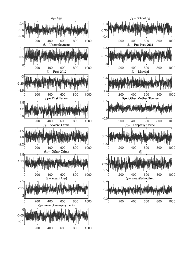
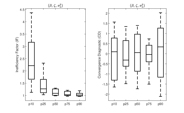
The mixing of the MCMC chain is extremely good as illustrated in Figure 3 which exhibits the trace plots of the parameters at the 75th quantile.1010 10 Note that the time-varying covariates (Age, Schooling and Unemployment rate) have been “demeaned” and that Age has been divided by 10. The parameter estimates must thus be interpreted accordingly. Trace plots at other quantiles are similar and not reported for the sake of brevity but they are available upon request. Figure 4 provides additional information on the performance of the MCMC chain. The left-hand-side figure depicts the boxplots of the inefficiency factors of the parameters (s, s and ) for each of the five different quantiles used in estimating the model. Except perhaps for the 10th quantile, all are reasonably close to one. Consistent with the simulation results, the parameter with the largest inefficiency factor at the 10th quantile is (not shown, see Table 2). The right-hand-side figure reports the boxplots of the convergence diagnostics of the parameter estimates for the same five specifications based on the first 10% and the last 40% values of the Markov chain (Geweke 1992). As depicted, all parameters have -scores within 2 standard deviation of the mean at the level or within standard deviation at level. All in all, the Markov chains behave satisfactorily and thus lend themselves to statistical inference.
Table 4 reports the posterior means and standard deviations at five different quantiles separately. To ease interpretation, the quantile-specific estimates are reported column-wise in increasing order. Row-wise, we distinguish the time-varying covariates from the time-invariant and the correlated random effects variables. Note that the correlated random effects specification does not include an intercept. This is to allow the identification of the two time-invariant policy variables, Pre-Post 2012 and Post 2012. The former, is equal to one if the detainee was incarcerated prior to 2012 and thus observed both before and after the implementation of the ‘‘tough-on-crime’’ policy. The latter is equal to one if a detainee’s first incarceration occurred during or after 2012, and thus always exposed to the policy. All other time-invariant variables are measured at first entry in the panel.1111 11 Recall from Table 3 that very few men are married. In addition, next to none report a change in their marital status in between incarcerations. Further, since the marital status of non-repeaters is not observed in the data we are constrained to use the information at entry in the panel. The estimates of the correlated random components associated with the individual mean Age, Schooling and Unemployment, , are all statistically different from zero regardless of the quantile. The individual-specific effects, , are thus highly correlated with the individual means of the time-varying variables. Omitting this correlation may therefore bias the model estimates and hence their intrinsic marginal effects and relative risks. This provides empirical support to the worthiness of incorporating correlated random effects within a quantile regression.
| Variable | ||||||||||||||||
|---|---|---|---|---|---|---|---|---|---|---|---|---|---|---|---|---|
| Mean | Std | Mean | Std | Mean | Std | Mean | Std | Mean | Std | |||||||
| Time varying covariates | ||||||||||||||||
| -Age | 0.426 | 0.183 | 0.099 | 0.083 | 0.123 | |||||||||||
| -Schooling | 0.116 | 0.047 | 0.025 | 0.021 | 0.032 | |||||||||||
| -Unemp Rate | 0.347 | 0.103 | 0.140 | 0.040 | 0.072 | 0.022 | 0.056 | 0.020 | 0.078 | 0.028 | ||||||
| Policy Variables (Time invariant) | ||||||||||||||||
| Pre-Post 2012 | 0.465 | 0.203 | 0.113 | 0.087 | 0.121 | |||||||||||
| Post-2012 | 0.522 | 0.224 | 0.125 | 0.097 | 0.134 | |||||||||||
| Other Time invariant covariates | ||||||||||||||||
| Married | 0.901 | 0.399 | 0.204 | 0.164 | 0.226 | |||||||||||
| Aboriginals | 0.634 | 0.295 | 0.148 | 0.121 | 0.197 | |||||||||||
| Oth. Mot. Ton. | 0.683 | 0.270 | 0.090 | 0.147 | 0.080 | 0.120 | 0.164 | |||||||||
| Violent Crime | 0.948 | 0.419 | 0.224 | 0.159 | 0.205 | |||||||||||
| Property Crime | 0.495 | 0.210 | 0.112 | 0.090 | 0.126 | |||||||||||
| Other Crime | 0.498 | 0.212 | 0.116 | 0.092 | 0.131 | |||||||||||
| Correlated Random Effects | ||||||||||||||||
| -Age | 0.456 | 0.195 | 0.105 | 0.085 | 3.286 | 0.123 | ||||||||||
| -Schooling | 0.127 | 0.051 | 0.027 | 0.023 | 0.034 | |||||||||||
| -Unemployment | 0.137 | 0.054 | 0.029 | 0.025 | 0.037 | |||||||||||
| 3.325 | 0.540 | 0.165 | 0.132 | 0.325 | ||||||||||||
The first noteworthy feature of the table is that all parameter estimates are statistically different from zero, except for the parameter associated with Other Mother Tongue. Thus detainees who report speaking a language other than English or French at home are no more and no less likely to eventually reoffend. A second interesting feature concerns the sign of the parameter estimates. Indeed, all are consistent with recent research on crime recidivism. For instance, Age and Schooling are associated with lower rates of recidivism (Bhuller et al. 2019) whereas being released during a period of high unemployment has been found to favour recidivism (Siwach 2018; Rege et al. 2019). Likewise, married men are less likely to reoffend whereas Aboriginal detainees are more likely to do so (Justice Canada 2017). The type of crime is also associated with recidivism. The estimates must be interpreted relative to traffic related crimes, which is the base or omitted category in our analysis. Clearly, sentences for Violent Crimes will be harsher and so the large parameter estimate presumably reflects an incapacitative effect. Finally, the parameter estimates of Post 2012 is larger than that of Pre-Post 2012 which suggests that the implementation of the “tough-on-crime” policy may have had a detrimental effect on recidivism.

As stated in Section 4, the parameter estimates such as those reported in Table 4 do not give the marginal effects. Yet, the latter are important from a policy perspective. Thus, while the parameter estimates vary considerably across quantiles, it is not clear that the marginal effects are equally sensitive since they depend both on the time-varying variables and the correlated random components. Figure 5 reports the average marginal effects computed according to equation (10), along with their highest posterior density intervals (HPDI).1212 12 The marginal effects for Age correspond to 1/10 of an additional year relative to the mean. Those for Unemployment and Schooling correspond to one additional year and one additional percentage point relative to their individual means, respectively. The remaining marginal effects correspond to a change in the indicator variables. Note that most marginal effects have a relatively flat profile between and and then exhibit a small kink between and . For instance, increasing Age by 1/10th reduces the probability of reoffending by 1% at the 10th quantile and by 1.6% at the 90th quantile. Similar results hold for Schooling (1% vs 2.0%), Married (0.3% vs 0.45%), and Violent Crime (5% vs 6.5%). Thus, for all three time-varying covariates the marginal effects increase by one half as we move from to . As for the time-invariant variables, their marginal effects all increase by at least 50% as we move from to . In particular, the marginal effects associated to First Nation, Property Crime and Other Crime exhibit a twofold increase. More importantly, the marginal effects of the two “tough-on-crime” variables increase manifold and in a steady fashion between and . Furthermore, the HPDI is relatively narrow in both cases. Hence, according to the parameter estimates associated with Pre-Post 2012, the probability of reoffending decreases from 78% at the 10th quantile to as little as 10% at the 90th. Likewise, the parameters of Post 2012 imply that the probability decreases from 79% to 14% at both extremes. These results are important from a policy perspective for two reasons. First, they imply that detainees from both groups are sensitive to the “tough-on-crime” policy, and even more so for those in the Post 2012 group. Consequently long-run recidivism (i.e. recidivism by the Pre-Post 2012 group between 2012-2017) can be addressed just as well as short-run recidivism (i.e. recidivism by the Post 2012 group between 2012-2017) by such policies. Second, the policy does not impact all detainees alike. Those in the lower quantiles are much more responsive than those in the upper quantiles.

In order to gain further insight into the sensitivity of recidivism to various covariates, we report the corresponding relative risks in Figure 6 (see equation (11)) along with their HDPI. Not surprisingly given the marginal effects, the relative risks are fairly constant for the first two or three quantiles (), with a few exceptions. Beyond the second or third quantiles, most increase or decrease sharply. The figure also shows which covariates influence recidivism most. Thus, while Age, Schooling and Unemployment Rate are associated with slightly different rates of repeat offenses, only those in the highest quantiles exhibit significantly different recidivism rates. On the other hand, marital status (Married), First Nation and types of crime (Violent, Property, Other) all have significantly higher or lower relative risks of reoffending as the case may be, and all exhibit a sharp change between the last two quantiles. Here, as with the previous figure, the results concerning the “tough-on-crime” variables are particularly interesting. Indeed, according to the figure all detainees were much less likely to reoffend in the post 2012 period, irrespective of whether they where first convicted prior to 2012 or after. As with the marginal effects, the policy appears to have had a larger impact on those in the lower quantiles. Thus for every quantile the risk of recidivism is much lower (and significantly different) for those who were exposed to the “tough-on-crime” policy. For instance, the 95% HPDI at quantile is for the Pre-Post 2012 group and for the Post 2012 group. On the other hand, the 95% HPDI at quantile for the two groups are and , respectively. In other words, for the lowest quantile (), exposure to the policy decreases recidivism by as much as and for the Pre-Post 2012 and Post 2012 groups, respectively. In contrast, for those in the highest quantile, , the Post 2012 group decreases its recidivism rate more than that of the Pre-Post 2012 ( vs ).
6 Conclusion
This paper presents a panel quantile regression model for binary outcomes with correlated random-effects (CRE) and proposes two MCMC algorithms for its estimation. By incorporating the CRE into the panel quantile regression for discrete outcomes, we move beyond the random-effects framework typically considered in the Bayesian quantile regression literature. The paper makes an important contribution to the literature on quantile regression for panel data and panel quantile regression for discrete outcomes. The two proposed MCMC algorithms are simpler to implement, but we prefer the algorithm that exploits block sampling of parameters to reduce the autocorrelation in MCMC draws. This blocked algorithm is tested in multiple simulation studies and shown to perform extremely well. We also emphasize the calculation of marginal effects in models with discrete outcome and explain its computation, along with those of relative risk and odds ratio, using the MCMC draws. Finally, we implement the proposed quantile framework to analyze crime recidivism in Quebec (a Canadian Province) for the period 20072017 using a novel data from the administrative correctional files. Amongst other things, we investigate the effect of the recently implemented “tough-on-crime” policy on the probability of repeat offense. Our results show that the policy negatively affects the probability of repeat offenses across quantiles and hence has been largely successful in achieving its objective. Besides, the results suggest that the CRE structure is relevant in modeling the probability of repeat offenses across quantiles.
This paper opens avenues for future research in several directions. The proposed framework can be readily extended to panel quantile regression models with continuous and other discrete response variables (e.g., count and ordinal outcomes). One may also consider the Hausman-Taylor version of CRE, where the individual-specific effects are related to only some of the time-varying and time-invariant regressors, and merge it with the panel quantile regression model for continuous or discrete outcomes. Besides, a dynamic relationship can be introduced to panel quantile regression models (with continuous or discrete outcomes) and the initial condition problems can be tackled using the CRE structure.
Conflict of interest
The authors declare that they have no conflict of interest.
References
- Abrevaya and Dahl (2008) Abrevaya J, Dahl CM (2008) The effects of birth inputs on birthweight: Evidence from quantile estimation on panel data. JBES 26(4):379–397
- Albert and Chib (2001) Albert J, Chib S (2001) Sequential ordinal modeling with applications to survival data. Biometrics 57:829–836
- Alhamzawi (2016) Alhamzawi R (2016) Bayesian model selection in ordinal quantile regression. Computational Statistics and Data Analysis 103:68–78
- Alhamzawi and Ali (2018) Alhamzawi R, Ali HTM (2018) Bayesian single-index quantile regression for ordinal data. Communications in Statistics Simulation and Computation pp 1–15
- Arellano (1993) Arellano M (1993) On the testing of correlated effects with panel data. Journal of Econometrics 59(1-2):87–97
- Arellano and Bonhomme (2016) Arellano M, Bonhomme S (2016) Nonlinear panel data estimation via quantile regression. The Econometrics Journal 19(3):61–94
- Bache et al. (2013) Bache SHM, Dahl CM, Christensen JT (2013) Headlights on tobacco road to low birthweight outcomes: Evidence from a battery of quantile regression estimators and a heterogeneous panel. Empirical Economcis 44(3):1593–1633
- Baltagi (2006) Baltagi BH (2006) Estimating an economic model of crime using panel data from North Carolina. Journal of Applied Econometrics 21(4):543–547
- Baltagi (2013) Baltagi BH (2013) Econometric Analysis of Panel Data. 5th Edition, John Wiley & Sons, Chichester
- Baltagi et al. (2003) Baltagi BH, Bresson G, Pirotte A (2003) Fixed effects, random effects or Hausman-Taylor? a pretest estimator. Economics Letters 79(3):361–369
- Baltagi et al. (2018) Baltagi BH, Bresson G, Chaturvedi A, Lacroix G (2018) Robust linear static panel data models using -contamination. Journal of Econometrics 202:108–123
- Barrodale and Roberts (1973) Barrodale I, Roberts FDK (1973) Improved algorithm for discrete linear approximation. SIAM Journal of Numerical Analysis 10(5):839–848
- Benoit and Poel (2010) Benoit DF, Poel DVD (2010) Binary quantile regression: A Bayesian approach based on the asymmetric Laplace distribution. Journal of Applied Econometrics 27(7):1174–1188
- Bhuller et al. (2019) Bhuller M, Dahl G, Loken K, Mogstad M (2019) Incarceration, recidivism and employment. Journal of Political Economy (forthcoming)
- Burda and Harding (2013) Burda M, Harding M (2013) Panel probit with flexible correlated effects: Quantifying technology spillovers in the presence of latent heterogeneity. Journal of Applied Econometrics 28(6):956–981
- Cameron and Trivedi (2005) Cameron AC, Trivedi PK (2005) Microeconometrics: Methods and Applications. Cambridge University Press, Cambridge
- Canay (2011) Canay IA (2011) A simple approach to quantile regression for panel data. The Econometrics Journal 14(3):368–386
- Chalfin and McCrary (2017) Chalfin A, McCrary J (2017) Criminal deterrence: A review of the literature. Journal of Economic Literature 55(1):5–48
- Chamberlain (1980) Chamberlain G (1980) Analysis with qualitative data. Review of Economic Studies 47:225–238
- Chamberlain (1982) Chamberlain G (1982) Multivariate regression models for panel data. Journal of Econometrics 18(1):5–46
- Chamberlain (1984) Chamberlain G (1984) Panel data. In: Griliches Z, Intriligator MD (eds) Handbook of Econometrics, vol 2, Elsevier, pp 1247–1318
- Chen (2007) Chen C (2007) A finite Smoothing algorithm for quantile regression. JCGS 16(1):136–164
- Chernozhukov et al. (2013) Chernozhukov V, Fernández-Val I, Hahn J, Newey W (2013) Average and quantile effects in nonseparable panel models. Econometrica 81(2):535–580
- Chib and Carlin (1999) Chib S, Carlin BP (1999) On MCMC sampling in hierarchical longitudinal models. Statistics and Computing 9:17–26
- Chib and Jeliazkov (2006) Chib S, Jeliazkov I (2006) Inference in semiparametric dynamic models for binary longitudinal data. Journal of the American Statistical Association 101(474):685–700
- Cornwell and Trumbull (1994) Cornwell C, Trumbull WN (1994) Estimating the economic model of crime with panel data. The Review of Economics and Statistics 76(2):360–366
- Dantzig (1963) Dantzig GB (1963) Linear Programming and Extensions. Princeton University Press, Princeton
- Dantzig and Thapa (1997) Dantzig GB, Thapa MN (1997) Linear Programming 1: Introduction. Springer, New York
- Dantzig and Thapa (2003) Dantzig GB, Thapa MN (2003) Linear Programming 2: Theory and Extensions. Springer, New York
- Davino et al. (2013) Davino C, Furno M, Vistocco D (2013) Quantile Regression: Theory and Applications. John Wiley & Sons, Chichester
- Davis (1991) Davis CS (1991) Semi-parametric and non-parametric methods for the analysis of repeated measurements with applications to clinical trials. Statistics in Medicine 10(12):1959–1980
- Devroye (2014) Devroye L (2014) Random variate generation for the generalized inverse Gaussian distribution. Statistics and Computing 24(2):239–246
- Galvao and Kato (2017) Galvao AF, Kato K (2017) Quantile regression methods for longitudinal data. In: Koenker R, Chernozhukov V, He X, Peng L (eds) Handbook of Quantile Regression, Chapman and HAll/CRC, New York, pp 363–380
- Galvao and Poirier (2019) Galvao AF, Poirier A (2019) Quantile regression random effects. Annals of Economics and Statistics (134):109–148
- Galvao et al. (2013) Galvao AF, Lamarche C, Lima LR (2013) Estimation of censored quantile regression for panel data with fixed effects. JASA 108(503):1075–1089
- Geraci and Bottai (2007) Geraci M, Bottai M (2007) Quantile regression for longitudinal data using the asymmetric Laplace distribution. Biostatistics 8(1):140–154
- Geraci and Bottai (2014) Geraci M, Bottai M (2014) Linear quantile mixed models. Statistics and Computing 24(461-479)
- Geweke (1991) Geweke J (1991) Efficient simulation from the multivariate normal and student- distributions subject to linear constraints and the evaluation of constraint probabilities. http://www.biz.uiowa.edu/faculty/jgeweke/papers/paper47/paper47.pdf, iowa City, IA, USA
- Geweke (1992) Geweke J (1992) Evaluating the accuracy of sampling-based approaches to the calculation of posterior moments. In: Bernardo JM, Berger JO, Dawid AP, Smith AFM (eds) Bayesian Statistics, vol 4, Clarendon Press, pp 169–193
- Geweke (2005) Geweke J (2005) Contemporary Bayesian Econometrics and Statistics. John Wiley & Sons
- Geyer (1991) Geyer CJ (1991) Markov chain monte carlo maximum likelihood. In: Kemramides EM (ed) Computing Science and Statistics: Proceedings of the 23rd Symposium on the Interface, Interface Foundation of North America, Fairfax Station, VA, USA, pp 156–163
- Ghasemzadeh et al. (2018a) Ghasemzadeh S, Ganjali M, Baghfalaki T (2018a) Bayesian quantile regression for analyzing ordinal longitudinal responses in the presence of non-ignorable missingness. METRON 76(3):321–348
- Ghasemzadeh et al. (2018b) Ghasemzadeh S, Ganjali M, Baghfalaki T (2018b) Bayesian quantile regression for joint modeling of longitudinal mixed ordinal contiuous data. Commincations in Statistics Simulation and Computation pp 1–21
- Gibbons and Hedeker (1993) Gibbons RD, Hedeker D (1993) Application of random-effects probit regression. Journal of Consulting and Clinical Psychology 62(2):285–296
- Graham et al. (2018) Graham BS, Hahn J, Poirier A, Powell JL (2018) A quantile correlated random coefficients panel data model. Journal of Econometrics 206(2):305–335
- Greenberg (2012) Greenberg E (2012) Introduction to Bayesian Econometrics. 2nd Edition, Cambridge University Press, New York
- Greene (2015) Greene W (2015) Panel data models for discrete choice. In: Baltagi BH (ed) The Oxford Handbook of Panel Data, Oxford University Press, New York
- Greene (2017) Greene WH (2017) Econometric Analysis. 8th Edition, Prentice Hall, New York
- Hausman (1978) Hausman JA (1978) Specification tests in econometrics. Econometrica 46(6):1251–1271
- Hausman and Taylor (1981) Hausman JA, Taylor WE (1981) Panel data and unobservable individual effects. Econometrica 49(6):1377–1398
- Jeliazkov and Rahman (2012) Jeliazkov I, Rahman MA (2012) Binary and ordinal data analysis in economics: Modeling and estimation. In: Yang XS (ed) Mathematical Modeling with Multidisciplinary Applications, John Wiley & Sons Inc., New Jersey, pp 123–150
- Jeliazkov and Vossmeyer (2018) Jeliazkov I, Vossmeyer A (2018) The impact of estimation uncertainty on covariate effects in nonlinear models. Statistical Papers 59(3):1031–1042
- Jeliazkov et al. (2008) Jeliazkov I, Graves J, Kutzbach M (2008) Fitting and comparison of models for multivariate ordinal outcomes. Advances in Econometrics: Bayesian Econometrics 23:115–156
- Joshi and Wooldridge (2019) Joshi R, Wooldridge JM (2019) Correlated random effects models with endogeneous explanatory variables and unbalanced panels. Annals of Economics and Statistics (134):243–268
- Justice Canada (2017) Justice Canada (2017) Indigenous overrepresentation in the criminal justice system. URL https://www.justice.gc.ca/eng/rp-pr/jr/jf-pf/2017/docs/jan02.pdf
- Karmarkar (1984) Karmarkar N (1984) A new polynomial time algorithm for linear programming. Combinatorica 4(4):373–395
- Kobayashi and Kozumi (2012) Kobayashi G, Kozumi H (2012) Bayesian analysis of quantile regression for censored dynamic panel data model. Computational Statistics 27(2):359–380
- Koenker (2004) Koenker R (2004) Quantile regression for longitudinal data. Journal of Multivariate Analysis 91(1):74–89
- Koenker (2005) Koenker R (2005) Quantile Regression. Cambridge University Press, Cambridge
- Koenker and Bassett (1978) Koenker R, Bassett G (1978) Regression quantiles. Econometrica 46(1):33–50
- Koenker and d’Orey (1987) Koenker R, d’Orey V (1987) Computing regression quantiles. JRSSC 36(3):383–393
- Kordas (2006) Kordas G (2006) Smoothed binary regression quantiles. Journal of Applied Econometrics 21(3):387–407
- Kozumi and Kobayashi (2011) Kozumi H, Kobayashi G (2011) Gibbs sampling methods for Bayesian quantile regression. Journal of Statistical Computation and Simulation 81(11):1565–1578
- Lalande et al. (2015) Lalande P, Pelletier Y, Dolmaire P, Raza E (2015) Projet, enquête sur la récidive/reprise de la clientèle confiée aux services correctionnels du Québec. Ministère de la sécurité publique du Québec (http://collections.banq.qc.ca/ark:/52327/2505967)
- Lamarche (2010) Lamarche C (2010) Robust penalized quantile regression estimation for panel data. Journal of Econometrics 157(2):396–408
- Link and Eaton (2012) Link WA, Eaton MJ (2012) On thinning of chains in MCMC. Methods in Ecology and Evolution 3:112–115
- Luo et al. (2012) Luo Y, Lian H, Tian M (2012) Bayesian quantile regression for longitudinal data models. Journal of Statistical Computation and Simulation 82(11):1635–1649
- MacEachern and Berliner (1994) MacEachern SN, Berliner LM (1994) Subsampling the Gibbs sampler. The American Statistician 48(3):188–190
- Madsen and Nielsen (1993) Madsen K, Nielsen HB (1993) A finite smoothing algorithm for linear estimation. SIAM Journal of Optimization 3(2):223–235
- Mehrotra (1992) Mehrotra S (1992) On the implementation of Primal-Dual Interior Point methods. SIAM Journal of Optimization 2(4):575–601
- Mundlak (1978) Mundlak Y (1978) On the pooling of time series and cross section data. Econometrica 46(1):69–85
- Omata et al. (2017) Omata Y, Katayama H, Arimura TH (2017) Same concerns, same responses: A Bayesian quantile regression analysis of the determinants for nuclear power generation in Japan. Environmental Economics and Policy Studies 19(3):581–608
- Owen (2017) Owen AB (2017) Statistically efficient thinning of a Markov chain sampler. Journal of Computational and Graphical Statistics 26(3):738–744
- Rahman (2013) Rahman MA (2013) Quantile regression using metaheuristic algorithms. International Journal of Computational Economics and Econometrics 3(3/4):205–233
- Rahman (2016) Rahman MA (2016) Bayesian quantile regression for ordinal models. Bayesian Analysis 11(1):1–24
- Rahman and Karnawat (2019) Rahman MA, Karnawat S (2019) Flexible bayesian quantile regression in ordinal models. Advances in Econometrics 40B:211–251
- Rahman and Vossmeyer (2019) Rahman MA, Vossmeyer A (2019) Estimation and applications of quantile regression for binary longitudinal data. Advances in Econometrics 40(B):157–191
- Rege et al. (2019) Rege M, Skardhamar T, Telle K, Votruba M (2019) Job displacement and crime: Evidence from norwegian register data. Labour Economics 61:101761
- Siwach (2018) Siwach G (2018) Unemployment shocks for individuals on the margin: Exploring recidivism effects. Labour Economics 52:231–244
- Soares and Fagundes (2018) Soares YM, Fagundes RA (2018) Interval quantile regression models based on swarm intelligence. Applied Soft Computing 72:474–485
- Wang (2012) Wang J (2012) Bayesian quantile regression for parametric nonlinear mixed effects models. Statistical Methods & Applications 21(3):279–295
- Wooldridge (2010) Wooldridge JM (2010) Econometric Analysis of Cross Section and Panel Data. 2nd Edition, MIT Press, Cambridge
- Yu and Moyeed (2001) Yu K, Moyeed RA (2001) Bayesian quantile regression. Statistics and Probability Letters 54(4):437–447
- Yuan and Yin (2010) Yuan Y, Yin G (2010) Bayesian quantile regression for longitudinal studies with nonignorable missing data. Biometrics 66(1):105–114