Abstraction-based Synthesis for Stochastic Systems with Omega-Regular ObjectivesJournal: the Nonlinear Analysis: Hybrid Systems Journal
Abstract
00footnotetext: This project was supported in part by the NSF under project #1749357.This paper studies the synthesis of controllers for discrete-time, continuous state stochastic systems subject to omega-regular specifications using finite-state abstractions. Omega-regular properties allow specifying complex behaviors and encompass, for example, linear temporal logic. First, we present a synthesis algorithm for minimizing or maximizing the probability that a discrete-time switched stochastic system with a finite number of modes satisfies an omega-regular property. Our approach relies on a finite-state abstraction of the underlying dynamics in the form of a Bounded-parameter Markov Decision Process arising from a finite partition of the system’s domain. Such Markovian abstractions allow for a range of probabilities of transition between states for each selected action representing a mode of the original system. Our method is built upon an analysis of the Cartesian product between the abstraction and a Deterministic Rabin Automaton encoding the specification of interest or its complement. Specifically, we show that synthesis can be decomposed into a qualitative problem, where the so-called greatest permanent winning components of the product automaton are created, and a quantitative problem, which requires maximizing the probability of reaching this component in the worst-case instantiation of the transition intervals. Additionally, we propose a quantitative metric for measuring the quality of the designed controller with respect to the continuous abstracted states and devise a specification-guided domain partition refinement heuristic with the objective of reaching a user-defined optimality target. Next, we present a method for computing control policies for stochastic systems with a continuous set of available inputs. In this case, the system is assumed to be affine in input and disturbance, and we derive a technique for solving the qualitative and quantitative problems in the resulting finite-state abstractions of such systems. For this, we introduce a new type of abstractions called Controlled Interval-valued Markov Chains. Specifically, we show that the greatest permanent winning component of such abstractions are found by appropriately partitioning the continuous input space in order to generate a bounded-parameter Markov decision process that accounts for all possible qualitative transitions between the finite set of states. Then, the problem of maximizing the probability of reaching these components is cast as a (possibly non-convex) optimization problem over the continuous set of available inputs. A metric of quality for the synthesized controller and a partition refinement scheme are described for this framework as well. Finally, we present a detailed case study.
Keywords:
finite-state abstractions, formal methods, interval-valued Markov chains, bounded-parameter Markov decision processes, stochastic systems.1 Introduction
The need for systems that are both complex and reliable is more critical than ever. Not only are the models describing these systems becoming increasingly complicated, but the tasks they are expected to perform also continue to grow in complexity. For example, the operating specification may combine an invariance and a reachability condition and require that the system will always return to a good state while always avoiding a bad state. Such specifications can be formally and unambiguously represented as, for instance, a Linear Temporal Logic (LTL) [1] specification, among other classes of symbolic languages. In this paper, we consider the class of -regular properties [2], a superset of LTL.
Recent research efforts in formal verification and synthesis have focused on the development of robust controllers to ensure that systems requirements are unequivocally met for broad classes of specifications and dynamics [3] [4] [5] [6] [7] [8] [9]. A general approach is to obtain a (non)deterministic finite abstraction of the continuous-state system, encode the specification as an appropriate transition system called an automaton, compute a product construction between the system abstraction and the automaton, and then synthesize a controller by solving graph-based problems on the product [10] [11]. The controller obtained from the finite abstraction is then mapped onto the original abstracted states. However, this basic recipe does not immediately work for stochastic systems because the random disturbances acting upon such systems add a quantitative component to the transitions between states in the form of transition probabilities, preventing the use of standard transition systems as finite abstractions for this framework. Typically, this limitation is overcome by using probabilistic finite transition systems as abstractions for stochastic systems [12] [13] [14] [15] [16]. Even though general synthesis procedures for such abstractions inherit ideas from approaches proposed in non-stochastic settings, the mathematical machinery required is quite different.
Indeed, for stochastic systems, satisfaction of a specification may never be fully guaranteed due to randomness. Therefore, the synthesis problem requires finding a control policy which maximizes or minimizes the probability of occurrence of some desired behavior from a given initial condition. In this work, we consider the problem of synthesizing a control policy for a discrete-time, continuous-state stochastic system subject to an -regular specification. Although the existence of optimal policies for this problem is not known, we seek to devise policies which are satisfactory with respect to a reasonable metric of quality. First, we consider the case when the control action is selected from a finite set of modes that the system can switch between at each time step. Then we consider the case when the control action is selected from a continuous set of possible inputs.
Recent literature demonstrated the effectiveness of Bounded-Parameter Markov Decision Processes (BMDP) as a tool for the synthesis of control policies in stochastic systems [16] [17]. Indeed, BMDPs are naturally amenable to finite-state abstractions of switched stochastic systems constructed from a finite partition of the continuous system domain. As each discrete state abstracts the behavior of an uncountably infinite number of underlying continuous states, the probabilities of transition between states are specified as intervals for each mode of the BMDP, rather than just a single number as in standard Markov Decision Processes. Solving for an optimal switching policy in the BMDP abstraction results in a near-optimal policy for the objective of maximizing or minimizing the probability of satisfying the specification with respect to the original abstracted states. The quality of this policy with respect to the original system states naturally depends on the quality and fineness of the continuous domain partition from which the abstraction is constructed.
In [16], the authors present an algorithm for computing switching policies that either minimize or maximize the probability of satisfying Probabilistic Computation Tree Logic (PCTL) specifications in a BMDP. The theory developed in [16] has been applied to linear systems with additive Gaussian noise subject to cosafe LTL specifications and was shown to be computationally efficient [18]. This BMDP-based technique was also recently implemented in the comprehensive verification and synthesis toolbox StocHy [19]. However, PCTL and cosafe LTL are strictly less expressive than the -regular logic and cannot articulate certain important liveness and persistence properties, such as the infinite repetition of some event [20]. A similar problem was solved in [21] for LTL specifications, but the proposed solution makes simplifying assumptions on the connectivity properties of the system’s abstraction which drastically reduces its scope of applicability. The synthesis of control strategies for interval Markov decision processes with multi-objectives that include -regular properties was discussed in [22]; however, the qualitative structure of the transition system is again assumed to be invariant, which alleviates key difficulties associated with the problem.
In this paper, we implement a procedure for computing switching policies in finite-mode discrete-time stochastic systems with the objective of minimizing or maximizing the probability of occurrence of any -regular property. We first create a partition of the continuous domain from which a BMDP abstraction of the system is generated. We then consider the Cartesian product between the BMDP abstraction and a Deterministic Rabin Automaton (DRA) representing the -regular property of interest for the maximization problem, or the complement of the property for the minimization problem. We prove that any such product BMDP induces a largest set of so-called Permanent Winning Component for a subset of all possible switching policies, and show that the probability maximization and minimization problems reduce to a reachability maximization task on these sets of states in the product BMDP. Note that our approach does not necessitate any assumption on the connectivity structure of the BMDP unlike in [21] and [22]. Furthermore, we introduce a quantitative measure capturing the quality of the switching policy designed in the BMDP abstraction when mapped onto the continuous abstracted states with respect to the objective of minimizing or maximizing the probability of fulfilling some specification in the original system. Finally, we propose a partition refinement technique inspired by our method in [23], which considered only the verification problem without inputs, in order to reach a desired level of optimality for the computed policy with respect to the continuous system states and progressively discard control actions which are guaranteed to be suboptimal. While no formal proof of the convergence of this technique is provided in this article, such refinement-based heuristics have shown to work remarkably well in practice and offer advantages in terms of scalability.
Expanding on the theory for finite-mode systems, we address the problem of synthesizing controllers for stochastic systems with -regular objectives from a continuous set of available inputs using finite-state abstractions. Related works discussed the synthesis of controllers for continuous input stochastic systems subject to subsets of -regular properties, such as Büchi objectives [24], using abstraction-based methods. Here, we specifically study the class of stochastic systems which are affine-in-disturbance and affine-in-input. We introduce Controlled Interval-valued Markov Chains (CIMC), which serve as abstractions for continuous input systems. We present an algorithm for constructing the largest permanent winning components in the product between a CIMC and a DRA. Then, we show that the reachability maximization step on these components can be formulated as an optimization program. The quality of the designed policy with respect to the original abstracted system and state-space refinement are discussed as well in this framework.
In brief, the novel contributions of this article over existing works, and in particular over our work on the verification of stochastic systems in [23], are as follows:
- •
We present a synthesis procedure for finite-mode discrete-time stochastic systems against -regular specifications, implemented in Algorithm 4. Our approach employs BMDP abstractions constructed from a partition of the continuous domain of the system, and we devise an automaton-based synthesis algorithm for BMDPs against -regular specifications from the results of Theorem 1 in conjunction with Algorithms 1 to 2. These algorithms perform a search of specific components of a BMDP which do not exist in abstractions without control actions along with the computation of policies generating these components, and therefore are more involved than the graph search algorithms found in [23]. The switching policy synthesized in the BMDP abstraction is then mapped onto the continuous abstracted states.
- •
We introduce a quantitative measure of the quality of the policy computed from the BMDP abstraction with respect to the original abstracted system states. The results in [23] are not concerned with the computation of switching policies and therefore do not propound such a measure. This metric is determined from the facts highlighted in Theorem 2.
- •
We develop a specification-guided refinement strategy on the partition of the system domain in Algorithm 3 to enhance the quality of the switching policy in refined BMDP abstractions of the dynamics. While an algorithm is presented in [23] for verification that is similar in spirit, major differences are found in the input of both algorithms, their termination criteria and the computations performed to select the states to be refined. This work additionally discusses some properties which are passed from coarser to refined abstractions, which is not done in [23].
- •
Next, we extend the techniques above to synthesize controllers for affine-in-disturbance, affine-in-input stochastic systems with a continuous set of permissible inputs. The control policy is computed by means of CIMC abstractions constructed from a partition of the system domain and mapped onto the continuous abstracted states as detailed in Algorithm 7. To this end, we present a synthesis procedure for CIMC abstractions arising from stochastic systems with the aforementioned structure that relies on Algorithms 5 and 6 and requires solving (possibly non-convex) optimization problems.
- •
For such systems with continuous input sets, we propose a refinement scheme for the domain partition to improve the quality of the computed controller with respect to the original abstracted states.
The paper is organized as follows: Section 2 introduces some preliminaries; Section 3 formulates the problem to be solved; Section 4 describes our controller synthesis strategy for finite-mode stochastic systems; Section 5 presents a controller synthesis algorithm for stochastic systems with a continuous set of inputs; Section 6 shows a case study; Section 7 concludes our work.
2 Preliminaries
A Deterministic Rabin Automaton (DRA) [11] is a 5-tuple where:
- •
is a finite set of states,
- •
is an alphabet,
- •
is a transition function,
- •
is an initial state,
- •
. An element , with , is called a Rabin Pair.
A DRA reads an infinite string or word over alphabet as an input and transitions from state to state according to . The resulting sequence of states or run is an accepting run if some states of are visited infinitely often and all states of are visited finitely often for some . A word is said to be accepted by if it produces an accepting run in . We call a set of words a property. The property accepted by is the set of all words accepted by .
A property over an alphabet is -regular if and only if it is accepted by a Rabin Automaton with alphabet (for more detailed definitions of -regular properties, see [11, Section 4.3.1]). In particular, all properties defined by a Linear Temporal Logic (LTL) formula are -regular. For example, the property “Eventually reach A", written in LTL as , has an equivalent -regular expression representation , where and are respectively the finite and infinite repetition operators. See [11] for a detailed description of the syntax and semantics of LTL.
A matrix is a transition matrix if for all , where is the th row and th column element of .
3 Problem Formulation
We first consider the discrete-time, continuous-state stochastic system
| (1) |
where is the state of the system at time , where is a finite set of modes, is a random disturbance (which could be mode-dependent), is a continuous map. Let be a labeling function, where is a finite alphabet and such that, for all , the subset of all states satisfying can be written as a finite union of subsets of , that is, . In Section 5, we extend this setup to allow for an infinite set of modes, i.e., a control input selected from a continuous set of inputs. An infinite random path satisfying (1) generates the word over . At each time-step , a mode is chosen and the random disturbance is sampled from a probability distribution with probability density function satisfying if . Then, a transition from state to state takes place according to the dynamics defined by mode . The set of all infinite paths of (1) is denoted by . A finite sequence of states produced by (1) is called a finite path. The set of all finite paths of (1) is denoted by . A function assigning a mode to each finite path in (1) is called a switching policy and the set of all switching policies of (1) is denoted by . For simplicity, we assume that all modes of are available at each state of . A policy induces a probability measure on the outcome space of infinite paths of (1), where is defined by the stochastic transition kernel assigning a probability measure to any state and mode on the space , with denoting the Borel -algebra on and such that , [25].
We denote by an arbitrary -regular property over alphabet and write as the probability that a word generated by a random path starting in satisfies property under policy (for a rigorous formalization of this probability, see, e.g., [14]). Our objective is to determine switching policies and that respectively minimize and maximize the probability of satisfying property for any path in the system and, by extension, for any initialization to of the system.
Problem 1: Given a system of the form (1), any initial state and an -regular property , find switching policies and that respectively minimize and maximize the probability of satisfying from , i.e.,
| (10) |
For complex specifications and dynamics, devising these exact optimal policies is likely to be intractable or infeasible due to the uncountably infinite number of states of the system’s domain. To determine a policy which is close to optimal, we consider an abstraction-based approach that consists in partitioning into a finite collection of states to construct a finite abstraction of the stochastic dynamics.
Definition 1 (Partition).
A partition of a domain is a collection of discrete states satisfying
- •
,
- •
where int denotes the interior. For any continuous state belonging to a state , we write .
For a partition of the domain of (1), the likelihood of transitioning from a state of to another state generally varies with the continuous state abstracted by from which the transition is actually taking place. Therefore, we cannot use partition to exactly abstract the system into a standard finite-mode Markovian model, such as an MDP. Instead, we propose producing a BMDP abstraction of the system where, for each action of the BMDP abstracting the behavior of (1) under some mode, the transition probabilities between states are constrained within some bounds, as depicted in Figure 1.
Definition 2 (Bounded-parameter Markov Decision Process).
A Bounded-parameter Markov Decision Process (BMDP) [17] is a 6-tuple where:
- •
is a finite set of states,
- •
is a finite set of actions, and the set of actions available at state is denoted by ,
- •
maps pairs of states and an action to a lower transition bound so that denotes the lower bound of the transition probability from state to state under action , and
- •
maps pairs of states and an action to an upper transition bound so that denotes the upper bound of the transition probability from state to state under action ,
- •
is a set of initial states,
- •
is a finite set of atomic propositions,
- •
is a labeling function from states to the power set of ,
and and satisfy for all , all , and
| (11) |
for all and all .
Definition 3 (BMDP Abstraction).
Given the system (1) evolving on a domain and a partition of , a BMDP is an abstraction of (1) if:
- •
, that is, the set of states of the BMDP is the partition ,
- •
, that is, the set of actions of the BMDP are the modes of (1),
- •
For all and action ,
(20) where for fixed denotes the probability that (1) transitions from to some state in under mode ,
- •
, i.e., the set of initial states of the BMDP is the partition ,
- •
For all and for any two states , it holds that , that is, the partition conforms to the boundaries induced by the labeling function.
For a given action, two continuous states belonging to the same discrete state of a BMDP abstraction may, in general, give rise to different transition probabilities. This fact is encoded in by the upper and lower transition probabilities.

In this paper, we do not present algorithms for computing BMDP abstraction of (1), which typically rely on overapproximating reachable sets; see [26] for such an approach. Thus, we assume that BMDP abstractions are available given a partition of for (1). However, we will focus on the problem of refining in order to obtain better BMDP abstractions.
Furthermore, we make the assumption that any state in of a BMDP can serve as an initial state. Denoting the set of all finite paths of a BMDP by , a switching policy for is a function assigning an action to all finite paths in . The set of all switching policies of is denoted by . Under a switching policy , the available actions in BMDP reduce to a single possibility at each time step, namely, that prescribed by the switching policy , inducing a (possibly countably infinite-state) Interval-valued Markov Chain (IMC), defined formally next. As will be discussed further, only finite-memory policies need to be considered in this work, which induce finite-state IMCs.
Definition 4 (Interval-valued Markov Chain).
An Interval-valued Markov Chain (IMC) is defined similarly to a BDMP with the difference that a single action (which is omitted in the defining tuple) is available.
The IMC induced by policy in BMDP is denoted by .
The state of an IMC evolves as follows: at each time step , the environment non-deterministically chooses a transition matrix compatible with the transition bound functions and of and the next transition occurs according to [27] 11 1 This is the Interval Markov Decision Process interpretation of IMCs.. A mapping from a finite path in to a transition matrix is called an adversary. The set of all adversaries of is denoted by . A unique probability measure is induced over the set of all infinite paths of IMC under adversary [11, Def. 10.10]. By extension, a probability measure is induced over the set of all infinite paths of BMDP under policy and adversary .
The probability of satisfying -regular property starting from initial state in IMC under adversary is denoted by .
The greatest lower bound and least upper bound on the probability of satisfying property starting from initial state in IMC are denoted by and respectively. When these bounds are the same for all states in a set of states of , we write and .
To design switching policies in BMDPs, it is crucial to note that a BMDP subject to a switching policy reduces to an IMC ; therefore, finding the probability of satisfying a specification from some initial state of amounts to solving a verification problem on an IMC. As discussed above, the probability of satisfying a specification in an IMC is not uniquely defined and depends on the instantiation of a non-deterministic adversary. Consequently, the verification of the IMC induced by a policy in a BMDP does not compute, in general, a fixed probability but an interval of satisfaction probabilities for all initial states of . The meaning of this interval is that the probability of fulfilling from state in is contained in for all possible adversaries of , that is, .
Because a switching policy in a BMDP returns an interval of satisfaction for all its initial states, it may not seem obvious which quantities to minimize or maximize when synthesizing policies in BMDP abstractions of continuous state systems. Note that a policy for a BMDP abstraction of (1) maps to a policy for (1) in the natural way, i.e., the control action prescribed by at a discrete state of is applied to all continuous states in (1). By virtue of being an abstraction of (1), it then holds that the exact probability of satisfying from any continuous initial state for (1) is contained within the bounds of the interval induced by policy for initial state in [16].
Therefore, given a BMDP abstraction of (1) generated from a partition of the domain , our approach to Problem 1 is to find policies and in that respectively maximize the lower bound probability (for the maximization objective) and minimize the upper bound probability (for the minimization objective) of satisfying for all initial states of .
Subproblem 1.1: Given a system of the form (1), a partition of its domain , a BMDP abstraction of (1) arising from , any initial state of and an -regular property , compute switching policies and that respectively minimize the upper bound probability and maximize the lower bound probability of satisfying in , i.e.,
If is a BMDP abstraction of (1), then a unique control action is assigned to all continuous states abstracted by some in . In this case, the quality of the policies and heavily depends on the quality and fineness of the partition of the domain . Indeed, because these policies only accommodate the extreme behaviors of all discrete states of , it is reasonable to assume that the computed policies may be suboptimal for a collection of continuous states abstracted by some . In this work, we address this problem by starting with a coarse partition of the system’s domain; then, we iteratively and selectively refine this partition so as to target discrete states that are at a higher risk of containing suboptimally controlled continuous states or are responsible for considerable uncertainty in the control of other states. As finer partitions result in larger abstractions to be analyzed, it is crucial to avoid performing unnecessary refinement in order to alleviate the state-space explosion phenomenon. The procedure terminates once a precision threshold which will be defined in further sections has been reached.
Subproblem 1.2: Given a system of the form (1) with a BMDP abstraction arising from a partition of the domain and an -regular property , refine the partition of until the computed switching policy reaches a user-defined threshold of quality with respect to the objective of minimizing or maximizing the probability of satisfying in (1).
After presenting solutions to Subproblem 1.1 and 1.2 in Section 4, we next investigate stochastic systems of the form
| (37) |
where is the state of the system at time , where is a continuous set of inputs, is a random disturbance whose probability density function is assumed to be independent of , is a continuous map. Here, a control policy is a function assigning a control action to each finite path in (37). The set of all control policies of (37) is denoted by as in the finite-mode system case.
The difficulty of establishing policies aiming to maximize or minimize the probability of satisfying a temporal property in (37) is highly dependent on the structure of the considered system. In this work, we restrict our attention to systems which are affine in input and disturbance, that is
| (38) |
As in the finite-mode case, we are interested in the design of a control policy that maximizes or minimizes the probability of satisfying an -regular property .
Problem 2: Given a system of the form (38), any initial state and an -regular property , find control policies and that respectively minimize and maximize the probability of satisfying from .
Solving this problem for an arbitrary property again involves a partition of the domain from which a finite-state abstraction of the system is constructed and analyzed. In this work, we introduce new abstraction tools called Controlled Interval-valued Markov Chains (CIMC) which differ from BMDPs in that the set of available actions is uncountably infinite. CIMCs are the abstractions of choice for systems of the form (38).
Definition 5 (Controlled Interval-valued Markov Chain).
A Controlled Interval-valued Markov Chain (CIMC) is a 6-tuple defined similarly to a BMDP with the difference that a continuous set of inputs replaces the finite set of actions .
Definition 6 (Controlled Interval-valued Markov Chain Abstraction).
Denoting the set of all finite paths in a CIMC by , a control policy for is a function assigning an input to all finite paths in . The set of all control policies of is denoted by . A policy applied to a CIMC induces an IMC denoted by .
Computing an optimal policy in a CIMC abstraction translates to computing a near-optimal policy when the former is applied to the original abstracted system. Thus, for all possible finite paths in , the goal is to find the input in the uncountable set that yields the most favorable IMC abstraction with respect to the desired objective. Note that, unlike in a BMDP abstraction, this problem offers an infinite set of available inputs to select from, ruling out the possibility of using an exhaustive search.
Subproblem 2.1: Given a system of the form (38), a partition of its domain , a CIMC abstraction of (38) arising from , any initial state of and an -regular property , compute the control policies and that respectively minimize the upper bound probability and maximize the lower bound probability of satisfying in , i.e.,
As our approach again relies on finite-state abstractions, finer partitions of the domain generally yield higher-quality control policies. Therefore, partition refinement for this case is discussed as well.
Subproblem 2.2: Given a system of the form (38) with a CIMC abstraction arising from a partition of the domain and an -regular property , refine the partition of until the computed control policy reaches a user-defined threshold of quality with respect to the objective of minimizing or maximizing the probability of satisfying in (38).
In the next section, we comprehensively detail our solution to the synthesis of switching policies for finite mode systems as formalized in Problem 1. Specifically, Subsections 4.1 and 4.2 focus on the computation of controllers for BMDP abstractions as stated in Subproblem 1.1, whereas Subsection 4.3 is concerned with Subproblem 1.2 and the refinement of BMDP abstractions for the synthesis of improved policies with respect to the abstracted system.
4 CONTROLLER SYNTHESIS FOR FINITE MODE SYSTEMS
4.1 BMDP CONTROLLER SYNTHESIS
In this subsection, we present the theory for addressing Subproblem 1.1. We adopt an automaton-based approach for computing maximizing and minimizing switching policies in a BMDP with respect to an -regular property . As discussed in Section 2, for every such property, there exists a corresponding DRA representation . Similar to [11, page 798] and [23] where the Cartesian product with a Markov Chain (MC) and an IMC are introduced, we define the product between a BMDP and a DRA.
Definition 7 (Product Bounded-Parameter Markov Decision Process).
Let be a BMDP and be a DRA. The product is a BMDP where:
- •
is a set of states,
- •
is the same set of actions of , where for all and for all ,
- •
- •
- •
is a finite set of initial states,
- •
is a set of atomic propositions, where and are the sets in the Rabin pairs of ,
- •
such that, for all atomic proposition , for all and for all , if and only if belongs to the set in the Rabin pairs of corresponding to .
In this product construction, the DRA is used as a finite-memory instrument that monitors all transitions occurring in and assesses whether the resulting path satisfies . Indeed, any random path in generates a unique path in which depends on the labels of the states of as per Definition 7. It follows that a switching policy in can be induced by inspecting the sequences of states generated in and choosing control actions accordingly.
Definition 8 (Generated Path in Product BMDP).
Consider a BMDP with set of states and labeling function and a DRA with set of states and transition function . A path in the product BMDP is said to be generated by the path in if it holds that .
Definition 9 (Induced Switching Policy).
Consider a BMDP , a DRA and a switching policy . Let be any finite path in . We denote by the path generated by in the product BMDP . The switching policy is said to be induced by a switching policy of if, for all , it holds that .
For a fixed switching policy of , the probability of satisfying in the induced IMC is equal to the probability of reaching a so-called Accepting Bottom Strongly Connected Component (BSCC) in the product IMC [23] defined below. The probability of reaching an accepting BSCC in is not uniquely defined and depends on the assumed transition values within the probability intervals selected by a non-deterministic adversary which induces a product MC .
Definition 10 (Product Interval-valued Markov Chain).
Let be an IMC and be a DRA. The product is an IMC defined similarly to a product BDMP with the difference that a single action (which is omitted in the defining tuple) is available.
Definition 11 (Markov Chain).
A Markov Chain (MC) is defined similarly to an IMC with the difference that the transition probability function or transition matrix of the Markov Chain satisfies for all and for all .
The probability of satisfying property in Markov Chain from initial state is denoted by .
Definition 12 (Induced Product Markov Chain).
A Product Markov Chain is said to be induced by an adversary of a product IMC if they share the same (for memoryless policies ), , , and , and for all , and all action , the transition probability function satisfies .
Definition 13 (Bottom Strongly Connected Component).
Given a Markov Chain with states , a subset is called a Bottom Strongly Connected Component (BSCC) of if
- •
is strongly connected: for each pair of states in , there exists a path such that , , and for with ,
- •
no proper superset of is strongly connected,
- •
, .
In words, every state in a BSCC is reachable from any state in , and every state in only transitions to another state in .
Definition 14 (Accepting and Non-Accepting Bottom Strongly Connected Component).
A Bottom Strongly Connected Component of a product Markov Chain is said to be accepting if:
is said to be non-accepting if it is not accepting.
A key observation is that, for any policy in induced by a policy in the product , the bounds on the probability of reaching an accepting BSCC from the initial states of are identical to the bounds on the probability of reaching an accepting BSCC from the initial states of according to Definitions 7 and 10 which ensure that the elements in the defining tuples of and are the same. Consequently, an analysis of the product is sufficient for approaching the synthesis problem.
Because -regular properties are closed under complementation, it should be noted that the problem of minimizing the upper bound probability of satisfying property in can be converted to the problem of maximizing the lower bound probability of satisfying the complement property with corresponding DRA . It follows that Subproblem 1.1 is solved by applying the same tools to both and .
Fact 1.
Let be a BMDP and be an -regular specification. We denote by the complement of property . For any initial state of and policy , it holds that
Therefore, our objective consists in computing a policy that maximizes the lower bound probability of reaching an accepting BSCC from all initial states of the resulting product IMC . We introduce the class of memoryless policies, which solely depend on the current state of the BMDP and will further prove optimal for our problem in the product BMDP , and the class of memoryless adversaries of an IMC.
Definition 15 (Memoryless Policy).
A policy of a BMDP is said to be memoryless if, for all finite paths of , it holds that .
Definition 16 (Memoryless Adversary).
An adversary of an IMC is said to be memoryless if, for all finite paths of , it holds that .
Before presenting a solution to Subproblem 1.1, we first recall some basic results established in [23] for the purpose of verification in IMCs which we then extend to compute switching policies in BMDPs.
For a given policy of and automaton , the sets of accepting and non-accepting BSCCs of the resulting product IMC depend on the assumed probability values for the transitions with zero lower bound and non-zero upper bound. Specifically, whether a zero or a non-zero value is assigned to these transitions directly affects the qualitative structure of the product IMC, and therefore its sets of accepting and non-accepting BSCCs, as a zero probability implies that a transition can never occur between the corresponding states, while a non-zero probability indicates that a transition is possible. When a non-zero probability is assumed for such a transition, we describe the transition as being “on", and we say that the transition is “off" in the scenario that a probability of zero is assumed. Nonetheless, it is shown in [23] that, for any product IMC, there exists a largest winning component and a largest losing component which can be created among all combinations of “on" and “off" transitions allowed by the transition bound functions of the product IMC. A winning component of a product MC is a set of states that reach an accepting BSCC with probability 1, while a losing component is a set of states that reach a non-accepting BSCC with probability 1.
Definition 17 (Winning Component).
[23] A winning component of a product MC is a set of states satisfying , where is the set of states belonging to an accepting BSCC in .
Definition 18 (Losing Component).
[23] A losing component of a product MC is a set of states satisfying , where is the set of states belonging to a non-accepting BSCC in .
Definition 19 (Largest Winning/Losing Components).
[23] A state of a product IMC is a member of the Largest Winning (respectively, Losing) Component if there exists a product MC induced by such that is a winning (respectively, losing) component.
Moreover, it was shown in [23] that the upper bound probability of satisfying in the IMC from state is equal to the upper bound probability of reaching the largest winning component of the product from state . Likewise, the lower bound probability of satisfying is found by solving a reachability problem on the largest losing component . These results naturally apply to product IMCs constructed from an IMC induced by a policy of a BMDP .
Fact 2 ([23]).
Let be an IMC induced by a switching policy of a BMDP and be a DRA corresponding to the -regular property . Let and be the largest winning and losing components of respectively. It holds that, for all initial states of ,
| (55) | ||||
The intuitive interpretation of this property is that any IMC has a “best-case" adversary and a “worst-case" adversary in the product that respectively maximizes and minimizes the probability of reaching an accepting BSCC for all initial states of simultaneously, since reachability probabilities are maximized by memoryless adversaries. These probabilities are equal to the upper bound and lower bound probabilities of satisfying from the initial states of . In an induced product MC corresponding to the best-case scenario, the set of winning components is as large as it can possibly be; in an induced product MC corresponding to the worst-case scenario, the set of winning components is reduced to the smallest possible set of permanent winning components.
Definition 20 (Permanent Winning Components).
[23] A state of a product IMC is a member of the Permanent Winning Component of if is a winning component for all product MCs induced by .
We further introduce the notions of permanent accepting BSCC, which is a subset of the permanent winning components of a product IMC. These sets will prove useful in subsequent sections.
Definition 21 (Permanent Accepting Bottom Strongly Connected Component).
[23] A state of a product IMC is a member of the Permanent Accepting BSCC of if belongs to an accepting BSCC for all product MCs induced by .
Now that these fundamental results regarding verification in IMCs, which will play a key role in the remainder of this section, have been stated, recall our primary objective which is to find switching policies and that respectively minimize the upper bound probability and maximize the lower bound probability of satisfying property from initial state in a BMDP . In light of the above facts, this amounts to enforcing the best possible worst-case scenario with respect to the probability of reaching an accepting BSCC in the product for the maximization case, or in the product for the minimization case. To this end, we first state in the following lemma that there exist sets of memoryless switching policies of resulting in the greatest possible set of permanent winning components in the corresponding induced product IMCs.
Lemma 1.
Let be a BMDP and be an -regular property with corresponding DRA . The set of policies of the product is denoted by and the set of memoryless policies of the product is denoted by . There exists a set of memoryless switching policies generating the set in such that, for all , where is the permanent winning component of , and, for all , the permanent winning component of is .
A constructive proof of this lemma is provided in the Appendix. The set is called the Greatest Permanent Winning Component of the product BMDP .
From Lemma 1, we infer that a maximizing policy with respect to in BMDP is induced by a policy in the product BMDP that effectively generates the set and, for all states not in , maximizes the lower bound probability of reaching this set; on the other hand, a minimizing policy with respect to in is induced by a policy achieving the same thing in , with denoting a DRA for the complement property of . Because optimal switching policies for reachability objectives are memoryless in BMDPs [28], it follows that the policy maximizing the lower bound probability of reaching an accepting BSCC in is the same for all initial states of . Likewise, the policy maximizing the lower bound probability of reaching an accepting BSCC in is the same for all initial states of .
Theorem 1.
Let be a BMDP, be an -regular property with corresponding DRA , and be the complement of with corresponding DRA . Let and be the greatest permanent winning component, respectively, of the product BMDP and , and and be the memoryless policies generating these sets in the corresponding product BMDP as defined in Lemma 1. A lower bound maximizing and upper bound minimizing switching policy and in with respect to are respectively induced by switching policies in and in such that
for all initial states of .
Proof.
We first prove equation (1). For all states belonging to , the lower bound probability of reaching an accepting BSCC under the defined policy is equal to 1, since , and is therefore maximized.
Next, in [23, Theorem 1], it was shown that a lower bound on the probability of reaching an accepting BSCC in a product IMC is achieved in an induced product MC with the smallest possible set of winning components admissible by , which is the permanent winning component of , for all states of . Furthermore, it was shown in [23, Lemma 9] that the probability of reaching an accepting BSCC in an induced product MC increases for all states of as more states are added to the set of winning components of while keeping all other transition probabilities identical. Assume the optimal policy does not belong to for some initial state of and denote by the permanent winning component of . As per the facts above, it follows that the probability of reaching an accepting BSCC from in the worst-case MC of has to be less than the probability of reaching an accepting BSCC from in the worst-case MC of , where allows the states in to be members of the permanent winning component and is the same as for all states outside of , which is a contradiction. Therefore, for all states of which are not in , a policy maximizing the lower bound probability of reaching a winning component has to belong to the set and generates the largest possible permanent winning component in .
Due to the properties of reachability problems in BMDPs, whose optimal policies are memoryless [28], there exists a policy in maximizing the lower bound probability of reaching simultaneously for all states which are not in , and, in particular, for all initial states of that do not belong to , concluding the proof of (1). Symmetric arguments combined with Fact 1 prove (1). ∎
This theorem shows that the desired policies are computed by solving a lower bound reachability maximization problem on a fixed set of states, which can be accomplished using the value iteration scheme presented in [16]. An algorithm for finding the sets and as well as their associated control actions are presented in the next subsection.
In this work, we also consider the policies and that respectively maximize the upper bound and minimize the lower bound probability of reaching a winning component for all states in a product BMDP . While these policies are not mapped onto the original system states, they will prove useful for assessing the quality of and in further sections. These are found by solving an upper bound reachability maximization problem on the Greatest Winning Component in (or ), whose existence is established in the lemma below.
Lemma 2.
Let be a BMDP and be an -regular property with corresponding DRA . The set of policies of the product is denoted by and the set of memoryless policies of the product is denoted by . There exists a set of memoryless switching policies generating the set in such that, for all , where is the largest winning component of , and, for all , the largest winning component of is .
Proof.
The set is called the Greatest Winning Component of the product BMDP .
Theorem 2.
Let be a BMDP, be an -regular property with corresponding DRA and be the complement of with corresponding DRA . Let and be the greatest winning component, respectively, of the product BMDP and , and and be the memoryless policies generating these sets in the corresponding BMDP as defined in Lemma 2. An upper bound maximizing and lower bound minimizing switching policy and in with respect to are respectively induced by switching policies in and in such that
| (88) | ||||
for all initial states of .
Proof.
As shown in [23, Theorem 1], an upper bound on the probability of reaching an accepting BSCC in a product IMC is achieved in an induced product MC with the largest possible set of winning components allowed by , which is the largest winning component of , for all initial states of . Hence, the same arguments as in the proof of Theorem 1 proves (88). Symmetric arguments combined with Fact 1 prove (2). ∎
We remark that replacing in (88) by the greatest accepting BSCC of does not change the validity of (88). The set contains all states which belong to an accepting BSCC for at least one induced product MC under at least one policy in . The proof of the existence of a set of control policies generating this set is similar to the first part of the proof of Lemma 1. This substitution can be done because, by definition, , and leads to algorithmic simplifications as the full set may not need to be computed explicitly. A similar reasoning holds by replacing with the greatest accepting BSCC of in (2). The components and as well as the control actions generating these components are found via a graph search, as detailed in the next subsections.
4.2 WINNING COMPONENTS SEARCH ALGORITHMS
Now, we present graph-based algorithms for finding the greatest permanent winning component of a product BMDP defined in Lemma 1. Furthermore, we show how to design a switching policy that effectively generates this greatest permanent component.
The search is decomposed in two parts: first, we determine a superset of the greatest permanent accepting BSCC, denoted by , of following Algorithm 1. The set contains all states which belong to a permanent accepting for some control policy in , and all such states are a part of as seen in the proof of Lemma 1. We call the superset of returned by this algorithm an extended greatest permanent accepting BSCC, denoted by . This set additionally satisfies . Although Algorithm 1 is driven by a search of the sets , our implementation allows us to find additional members of in some instances.
Then, by using an iterative technique which alternates between a graph search and a reachability maximization step in Algorithm 2, one can find the set of states which are not members of but for which the lower bound probability of reaching an accepting BSCC is equal to 1 nonetheless for some control policy, and effectively create .
4.2.1 GREATEST PERMANENT BSCC SEARCH ALGORITHMS
We now detail an algorithm for finding an extended greatest permanent accepting BSCC of a product BMDP .
We introduce the following notations and terminology: a set of states in a product is said to be accepting if it satisfies the acceptance condition in Definition 14 and is said to be non-accepting otherwise. A state of with labeling function is said to be Rabin accepting with respect to the Rabin pair of if ; is said to be Rabin non-accepting with respect to the Rabin pair of if . A Rabin accepting state with respect to the pair is said to be unmatched in a set of states if, for all , , and it is said to be matched otherwise. is a set containing all sets of actions allowed for each state in a set , that is, if , , then, . is a function which outputs the set of states in which have a non-zero probability of transition to for at least one adversary under all actions in . In addition, this function removes all actions from the sets in for which a transition to is possible under at least one adversary and returns the updated set of allowed actions for each state of .
We provide a short description of the algorithm: Algorithm 1 first finds the largest possible set of Strongly Connected Components (SCC), denoted by , that can be constructed in the product BMDP in line 4 and 5 assuming all actions are available, as the greatest permanent BSCCs are a subset of these by Definition 13. Set is determined by applying a standard SCC search techniques on the graph defined in line 4.
Then, the algorithms iteratively remove the actions and states which prevent these SCCs from being a permanent BSCC, that is, actions and states which allow for a transition outside of the SCCs, as captured by line 9. Note that a state is discarded in set once its action set is empty. Then, new SCCs are computed with the remaining states and actions in line 12. If the algorithm finds an SCC which does not allow any transition outside of for any state and action available, then it is potentially a member of (line 13).
Next, the acceptance status of SCC is checked at line 14. This is done by inspecting the states belonging to the SCC and comparing them with Definition 14. If is not accepting, states which can revert the acceptance status of are removed and new SCCs are computed with the remaining states in line 23. Otherwise, the algorithm enters the if-statement in line 14 for a further analysis of .
An additional condition for to be a part of is that no subset of states of can form a non-accepting BSCC under any scenario allowed by the transition intervals of the product BSCC. Too make sure that no subset of can form a non-accepting BSCC, we choose control actions for the states in that maximize the lower bound probability of reaching the unmatched Rabin accepting states contained in in line 14 to 17. If this lower bound is zero for some subset of , then these states could potentially form a non-accepting BSCC inside for some assignment of the probabilities under all available actions. The set of all such states is denoted by . If is empty, the algorithm found a control policy that guarantees to be accepting for all possible adversaries of the induced product IMC, since no state of can form a BSCC which doesn’t contain at least one of the unmatched accepting states, and is added to in line 18. Otherwise, the SCCs which can be formed by the states in and by the states in with the remaining actions are computed and added to in line 20.
We offer the following reasoning as a proof sketch for the correctness of the algorithm , i.e, to show that the output of Algorithm 1 satisfies the chains of inequalities : for a set of states to belong to a permanent BSCC of a given kind in a product IMC, the following conditions must hold: 1) its constituents are not allowed to transition outside of under any adversary, 2) its constituents have to be reachable from one another under all adversaries, 3) its constituents have to fulfill the requirements for accepting and non-accepting BSCCs defined in Definition 14, 4) no subset of is allowed to form a BSCC of the opposite acceptance status under any adversary. Condition 1) is guaranteed by lines 7 to 10; Condition 2) is not enforced and is the reason for outputting a superset of . This is because, as long as the other 3 conditions are fulfilled, the states in the set will still be permanently winning,, although the transition bounds within might allow these sets to be winning via different scenarios that are not only a BSCC formed by all the states of (e.g. a subset of always transitioning to a another subset of forming a BSCC); Condition 3) is enforced by the if-statement in line 14 and the corresponding else-statements of lines 22 to 24; Condition 4) is imposed by the remainder of the main for-loop. Lastly, the algorithm iteratively removes the minimum number of actions and states causing a set to violate one of these conditions and analyze all of the remaining states, ensuring that the procedure does not skip any permanent component. Note that none of the removed states could form a permanent BSCC between each other under any policy. Indeed, if these states did not belong to a common SCC in , this would be a contradiction. Therefore, by virtue of this fact, Algorithm 1 does not “miss" any permanent BSCCs and it must hold that . Moreover, the previous discussion regarding Condition 2 ensures that all states in are still permanently winning, guaranteeing that and concluding the proof sketch.
This algorithm can be adapted to determine an extended greatest accepting by replacing all instances of the function with the function , where returns the set of states of which have a non-zero probability of transition to for all adversaries under all allowed actions. This function also removes all actions from for which a non-zero probability of transition to exists under all adversaries of the induced IMC and returns the updated set of allowed actions. In addition, all mentions of the term “lower bound" have to be replaced with “upper bound". The extended set is such that .
4.2.2 GREATEST PERMANENT COMPONENTS SEARCH ALGORITHMS
Next, we present an algorithm which constructs the greatest permanent winning components in a product BMDP once an extended greatest permanent BSCC has been found.
In a product IMC , some states which are not in a permanent BSCC can still be a part of the permanent winning component of , as discussed in the second part of the proof of Lemma 1. These states are those which belong to a set of states such that no transition outside the union of and the permanent BSCCs of is possible for any adversary, and such that no subset of can form a non-accepting BSCC status under any adversary. We can further classify these states into permanent sink states, which cannot be a part of a BSCC under any scenario but transition to another winning set of state with lower bound probability 1, and states which allow non-deterministic scenarios where the state is sometimes a sink state with respect to another permanent winning set of states and sometimes a part of a winning component that reaches a non permanent accepting BSCC with probability one. The examples below, illustrated in Figure 2, present situations where these scenarios can occur.
Example 1.
Consider three states , and of a product IMC such that and form a permanent BSCC, with . Furthermore, and . Clearly, is not a member of the BSCC encompassing and ; yet, always transitions to either or with probability probability 1 and is therefore a permanent sink state.
Now, consider two states and such that , and . While is a permanent BSCC, is neither a permanent sink state nor a permanent BSCC. However, all adversaries of the product IMC make either a sink state with respect to or a BSCC with itself.
Consequently, we describe a procedure in Algorithm 2 that finds all states in a product for which a control policy induces one of the aforementioned scenarios given extended greatest permanent BSCCs .
We explain the main features of this algorithm: first, the greatest permanent winning component is initialized to the extended greatest permanent accepting BSCCs in line 3. Then, in line 5, the lower bound probability of reaching this component is maximized in the product BMDP to reveal the states which can be rendered permanent sinks with respect to , as these states yield a lower bound of 1 of reaching the component. The sink states are added to in line 8.
Next, we define the greatest potential accepting BSCC of a product BMDP, which are computed by taking the set difference between the greatest winning BSCC and the greatest permanent winning BSCC. States in are those which could engender the second type of permanent components previously discussed. If happened to contain a permanent sink state found in line 8, we compute the greatest accepting and non-accepting BSCC as well as their associated allowed actions with the remaining states in line 10 to update .
Then, in lines 12 to 17, for all BSCCs which can be created in , we check whether there exists a policy such that no state of can transition outside of the union of and the current version of the greatest permanent winning component for any instantiation of the resulting transition intervals. If such a policy does not exist, states and actions for which a transition outside of the aforementioned set is possible are removed from and the BSCCs which can be created inside the greatest BSCC of the remaining states are added to the list of BSCCs to inspect in line 19. On the other hand, if only contains valid states and corresponding actions, the algorithm enters the else-statement in line 20, where we need to choose a policy for the states in which additionally does not allow the existence of a non-accepting BSCC within under any adversary.
This step is done similarly as in Algorithm 1 by maximizing the lower bound probability of reaching the unmatched Rabin accepting states in and removing the states yielding a lower bound probability of . If no such state is found, then we designed a policy that effectively makes either a set of sink states or an accepting BSCC for all adversaries, and the states of are added to the greatest permanent winning component . This process is described in line 21 to 28.
In the case that new states were added to upon execution of the reachability maximization step and the graph search, which is checked in line 31 to 33, we return to the beginning of the while-loop and repeat this process with the augmented version of the greatest permanent winning component, as it could now allow previously discarded states to become permanently winning. Otherwise, the loop is exited and the algorithms return the true set with its associated control actions.
A slight modification of Algorithm 2 can be employed to compute the greatest set defined in Lemma 2. However, in this paper, we solely use the greatest accepting BSCC as our target set for computing the upper bound maximizing and lower bound minimizing policies and , as explained in Subsection 4.1.
In summary, we develop a procedure for computing policies that either maximize the lower bound probability or minimize the upper bound probability of satisfying an arbitrary -regular property in a BMDP. To this end, we show that these policies are induced by policies in the product between the BDMP and a DRA encoding the specification of interest for the maximization objective, or a DRA encoding the complement of the specification for the minimization objective. In Lemma 1, we remarked that a product BMDP always possesses a greatest permanent winning component. In Algorithms 1 and 2, we devise graph-based techniques for determining this component as well as the corresponding control actions for the states composing them. Finally, we show in Theorem 1 that, for the remaining states in the product BMDPs, the optimal policies are found by carrying out a lower bound reachability maximization computation on the greatest permanent winning component.
4.3 STATE SPACE REFINEMENT
4.3.1 QUALITY OF COMPUTED POLICY
In the previous subsections, we implemented a technique for computing an optimal switching policy in a BMDP subject to an -regular specification. However, recall that, in the problem at hand, BMDPs are used as abstractions of the underlying system (1) with respect to a partition of the system’s continuous domain. Therefore, as each state of the BMDP abstracts the behavior an infinite number of continuous states of (1), the switching policy derived in the BMDP abstraction is likely to be suboptimal when mapped onto the original system.
Here, we provide a measure of the suboptimality of the control strategy computed in a BMDP abstraction with respect to the abstracted system. While the discussion in this section focuses on optimality for the probability maximization problem with respect to specification , the same facts can straightforwardly be applied to the dual minimization problem by replacing the instances of , and with , and respectively, where is a DRA representing the complement specification .
The value iteration algorithm used to design the policies and discussed in Theorem 1 and Theorem 2 provides useful information amenable to a quantitative measure of the quality of the lower bound maximizing policy . In particular, for all states , the algorithm determines a lower bound on the maximum lower bound probability of reaching an accepting BSCC achievable from over all memoryless policies of choosing the lower bound maximizing action at state , and an upper bound on the maximum upper bound probability of reaching an accepting BSCC achievable from over all memoryless policies of choosing action at state for all actions . Denoting these lower and upper bounds by and respectively for action , and the set of memoryless policies of by , this is formally stated as
where the subscript refers to the lower bound maximizing action and, for all actions ,
| (113) |
where is a slight abuse of notation denoting the objective of reaching an accepting BSCC — which is generally not a fixed set of states as discussed in previous sections — in the product IMC .
Therefore, we introduce the suboptimality factor of state with respect to the lower bound maximizing policy in the product BMDP which is defined as
The quantity represents an upper bound on the maximum improvement in the probability of satisfying , using a memoryless policy with respect to the DRA states, any continuous state in could achieve by choosing another fixed action from the one prescribed by when the product state is , as the maximum satisfaction probability attainable when applying a different action is upper bounded by . Therefore, the smaller is, the more certain we are that is close to the best memoryless (in the product) policy for all states in when the automaton state is .
Furthermore, the bounds computed by the value iteration algorithm can additionally be used to show that certain actions are suboptimal or optimal at a given state of a product BMDP and, by extension, that the modes represented by these actions are suboptimal or optimal for some continuous states of the abstracted system for policies that are memoryless in the product. By comparing these bounds for all actions in an action space of a given state of the product BMDP , some of these actions may appear to surely perform worse or better than others at that particular state, as illustrated in the example below.
Example 2.
Consider a state of the product BMDP with a set of actions , and . Suppose the probabilities of reaching an accepting BSCC from under all 3 actions are described by the following intervals:
- •
- •
- •
where the lower bounds correspond to a lower bound on the maximum lower bound probability of reaching an accepting BSCC from state achievable over all memoryless policies of choosing the corresponding action at state , and the upper bounds correspond to an upper bound on the maximum upper bound probability of reaching an accepting BSCC from state achievable over all memoryless policies of choosing the corresponding action at state .
Although action maximizes the lower bound probability of reaching an accepting BSCC at , it appears that some continuous states of could potentially produce a higher probability — up to — of reaching an accepting BSCC under action , since a non-deterministic scenario of the product BMDP allows for this probability to occur under some policy choosing . However, under no memoryless policy and adversary can action generate a higher probability of reaching an accepting BSCC than action , since , and can therefore be discarded.
In spite of action being removed, the suboptimality factor of with respect to in this case is , as there still exists an action achieving a higher upper bound probability of reaching an accepting BSCC, namely with , than the lower bound probability of reaching an accepting BSCC under the lower bound maximizing action, namely with .
Definition 22 (Optimal/Suboptimal Action).
Consider a state of a product BMDP with a set of actions . Let us denote by a lower bound on the maximum lower bound probability of reaching an accepting BSCC from achievable over all memoryless policies of choosing action at state , and by an upper bound on the maximum upper bound probability of reaching an accepting BSCC from achievable over all memoryless policies of choosing action at state . An action is said to be suboptimal for state with respect to if there exists an action , , such that . An action is said to be optimal for state with respect to if, for all , , .
Definition 23 (Optimal/Suboptimal Mode).
Let be any finite path of (1) such that the word produces a run in automaton corresponding to property , where and . Let us denote by a lower bound on the maximum (respectively, minimum) probability of an infinite path with prefix to satisfy in (1) over all policies of (1) choosing mode for path , and by an upper bound on the maximum (respectively, minimum) probability of an infinite path with prefix to satisfy in (1) over all policies of (1) choosing mode for path . When the objective is to maximize (respectively, minimize) the probability of satisfying , a mode is said to be suboptimal for state with respect to automaton state and the set of modes if there exists a mode , , such that (respectively, ). A mode is said to be optimal for state with respect to automaton state and the set of modes if, for all , , (respectively, ).
If the set of actions of state contains an optimal action, then the suboptimality factor is set to 0.
4.3.2 REFINEMENT PROCEDURE
Now that a quantitative measure for the quality of the computed switching policy has been introduced, our next objective is to design a domain partition refinement scheme to address Subproblem 1.2 and achieve a user-defined level of optimality. In order to mitigate the state-space explosion phenomenon, the refinement algorithm should specifically target the states causing the most uncertainty in the domain partition.
We define the greatest suboptimality factor as
| (122) |
which can be used as a natural precision criterion for a given domain partition . A low factor ensures that no state in the original system is poorly controlled under the switching policy computed in the BMDP abstraction arising from . Looser notions of optimality, such as the average suboptimality factor or the fraction of states below a fixed optimality threshold, are less sensitive to outliers and can alternatively be considered. We denote the desired suboptimality target by . Note that a target equal to requires to find an optimal action for all states in in the case of maximization or in for the case of minimization.
Formally, a partition is a refinement of a coarser partition if all states in is equal to the union of a set of states in . In the general case, abstractions constructed from a refinement of will exhibit a lesser degree of non-determinism than abstractions constructed from , allowing for the computation of higher-quality controllers with respect to the abstracted system.
Definition 24 (Partition Refinement).
A partition is a refinement of a partition if, for all states , there exists a set of states in such that .
The proposed refinement procedure to achieve a target precision is inspired by our technique in [23] where refinement was conducted for the purpose of verification in an IMC and whose main features are extended to the synthesis problem at hand. This new procedure is based on a heuristical scoring of the states in a partition which highlights the regions of the state-space causing the most uncertainty with respect to the specification of interest and the set of actions at hand. Specifically, this score aims to capture how differently a partition state behaves between the extreme cases induced by the two maximizing (or minimizing) policies previously discussed, as well as how much this state influences other states which are known to be suboptimaly controlled.
Our scoring algorithm is presented in Algorithm 3 and is summarized as follows: first, we take as input a “best-case" product MC and a “worst-case" product MC . For the case of maximization, the worst-case product MC is a worst-case product MC induced by the IMC with respect to the objective of reaching an accepting BSCC, while the best-case product MC is a best-case product MC induced by the IMC . Similarly, for the case of minimization, the worst-case product MC is a worst-case product MC induced by the IMC with respect to the objective of reaching an accepting BSCC, while the best-case product MC is a best-case product MC induced by the IMC . Again, the aforementioned MCs are automatically constructed when applying the reachability value iteration algorithm used in Algorithms 1 and 2 and for designing the two maximizing (or minimizing) policies.
Next, for all state of the product BMDP (or ) whose suboptimality factor is greater than the target , we compute the probability of reaching any state from in the MC on line 7 using the results in [29]. Then, for all states of the product BMDP that do not belong to a permanent component (as these do not require refinement), the quantity is added to the score of the partition state on line 10, where and are the rows corresponding to state in the transition matrices of and respectively. The term aims to capture how differently state behaves in the two extreme MCs, while is a term associated with how much state affects state . Finally, from line 10 to 13, we additionally increment the score of states which have the potential of changing the qualitative connectivity structure of the “best" and ”worst" case scenarios. These states are those which belong to a BSCC that is present in one of the scenarios and not in the other and have the potential of confirming or invalidating the existence of these BSCCs, that is, states which have an outgoing transition with a zero lower bound and a non-zero upper bound for at least one available (non-suboptimal) control action.
Once a score is attributed to each state of via Algorithm 3, states with a score above a user-defined threshold are refined to generate a finer partition . A new switching policy is computed in a BMDP abstraction constructed from , and more refinement steps are subsequently applied if necessary. The procedure terminates once the optimality factor becomes less than the target .
It should be noted that a product IMC generally does not induce a unique worst-case and best-case MC, but rather induces sets of possible worst-case and best-case MCs yielding the same probabilities of reaching an accepting BSCC from all states [23]. Therefore, the choice of inputs for Algorithm 3 may not be unique. As previously discussed, we choose to input the MCs computed in the process of designing the control policies for the BMDP. Although selecting other MCs is possible, we claim that the design of Algorithm 3 renders the effect of choosing other input MCs negligible in the long-term behavior of the refinement-based synthesis algorithm in all but pathological cases. The reasoning behind this claim is that a lot of discrepancies between different worst-case (or best-case) MCs occur in the transitions within permanent winning or losing components which belong to the set defined in Line 5 of Algorithm 3, as the existence of these components depend on the qualitative structure of the IMC and not on the exact transition values, and have no influence on the computation of the refinement scores. Other large discrepancies between different such MCs may be found in the potential BSCCs stored in set in Line 4. However, the relative difference captured by the term at such states is likely to be similar regardless, causing only a minor variation in refinement scores for two different input MCs, and the set may quickly become empty after a few iterations of the refinement algorithm as the states causing this set to exist, namely states without zero lower bound and non-zero upper bound, are heavily targeted in Line 12 to 14. Finally, different transitions between two worst-case (or best-case) MCs can be found outside of the aforementioned sets, but this scenario is improbable for abstractions computed from dynamical systems with continuous state-spaces. Indeed, this would require for at least two states outside these sets to have the exact same probability of reaching an accepting or a non-accepting BSCC in the extremal assignments of the transition probabilities, which is highly unlikely when using transition bounds derived from integrals over continuous sets. Such a scenario may be encountered on coarse abstractions with very few states that are all bound to be refined no matter which best or worst-case MC is chosen, and finding such states with equal reachability probabilities in high-dimensional MCs would be implausible or an isolated event with little impact on the refinement algorithm.
The fact that a partition is a refinement of a partition allows us to make inferences about the properties of the states in from the synthesis computations previously performed on the states in . First, as discussed in the previous subsection, not all actions allowed in may need to be considered in the refined partition when computing a new switching policy. Indeed, given a partition of a state , it follows that a certainly suboptimal action with respect to the action set of a product state will also be suboptimal with respect to all and can be eliminated in the synthesis procedure applied to .
Proposition 1.
Let be a BMDP abstraction constructed from a partition of the domain of (1), be a DRA corresponding to specification , and be a refinement of . Let , be a partition of state . If action is suboptimal for state with respect to in the product BMDP , then the mode of (1) represented by action is suboptimal for all with respect to the automaton state and the set of available modes, and, in particular, for all , .
Proof.
The proof assumes the objective of synthesis to be the maximization of the probability of satisfying . We denote by an upper bound on the maximum upper bound probability of reaching an accepting BSCC in from achievable over all memoryless policies choosing action at state . The assumption that is suboptimal with respect to in implies that there exists an action with a known a lower bound on the maximum lower bound probability of reaching an accepting BSCC in from achievable over all memoryless policies choosing action and such that . Therefore, by virtue of being an abstraction of (1), , it follows that , where and are a lower bound and an upper bound on the maximum probability that an infinite path of (1) with prefix , , such that the word produces a run , with , satisfies over all the (memoryless in the product) policies of (1) choosing the modes represented by actions and respectively at path . It follows that the mode represented by action is suboptimal for all with respect to automaton state and the set of available modes. In particular, this statement is true for all , , since , proving the proposition. Symmetric arguments prove this proposition in the case of minimization. ∎
Furthermore, out of the remaining actions, only a subset of them may be retained for the qualitative problems of constructing the largest and permanent components in using Algorithms 1 and 2. Indeed, all actions in which were discarded during the graph search for could not, under any policy and adversary, generate a winning component in . Therefore, based on this fact, we can define the set of actions used specifically for the component graph search and containing all actions which, at state , allowed for the existence of with respect to the partition .
Proposition 2.
Let be a BMDP abstraction constructed from a partition of the domain of (1), be a DRA corresponding to specification , be a DRA corresponding to complement specification , and be refinement of a partition . If state is not a member of in the product BMDP (respectively, ) under any memoryless policy of (respectively, ) such that , then, for all , the probability that an infinite path with prefix , , such that the word produces a run , with in automaton , satisfies is strictly less than 1 (respectively, strictly greater than 0) for all policies of (1) choosing the mode represented by action at state . In particular, this statement is true for all , , where , , is a partition of state .
Proof.
The proof assumes the objective of synthesis to be the maximization of the probability of . If state is not a member of under any memoryless policy such that , then it must be true that , where is an upper bound on the probability of to reach an accepting BSCC in under all memoryless policies such that . Therefore, by virtue of being an abstraction of (1), it follows that the probability of an infinite path with prefix , , such that the word produces a run , with in automaton to satisfy is upper bounded by for all policies of (1) choosing the mode represented by action for the path and is thus strictly less than 1. In particular, this statement is true for all , , since , proving the proposition. Symmetric arguments prove the proposition with respect to the minimization objective. ∎
An analogous proposition can be established with respect to the greatest BSCCs for Algorithm 1.
We also remark that any state belonging to the greatest permanent winning components of a BMDP abstraction constructed from a partition has to belong to the greatest permanent components with respect to a refined partition if the same control action applied to all in the abstraction resulting from is applied to all their refinement states .
Proposition 3.
Let be a BMDP abstraction constructed from a partition of the domain of (1), be a DRA corresponding to specification , be a DRA corresponding to complement specification , and be refinement of a partition . A policy of induced by a policy in (respectively, in the case of minimization) generating the greatest permanent winning component of (respectively, of ) selects an optimal mode (with the appropriate mode/action correspondence) for all such that with respect to the automaton state and the set of available modes, and, in particular, for all , , where , , is a partition of state .
Proof.
The proof assumes the objective of synthesis to be the maximization of the probability of . A policy generating in ensures that for all . The policy in induced by applied to all such that when the automaton state is with the appropriate mode/action correspondence guarantees that, for all such , the probability of an infinite path with prefix , , such that the word produces a run , with in automaton to satisfy is equal to 1, by virtue of being an abstraction of (1). Therefore, selects an optimal mode for all such . In particular, this statement is true for all , , since , proving the proposition. Symmetric arguments prove the proposition with respect to the minimization case. ∎
Therefore, by pruning all states which were a member of in an abstraction constructed , since an action engendering a fixed probability of reaching an accepting BSCC equal to 1 is known for such states, we can reduce the effective set of states for which a controller has to be synthesized in the abstraction arising from a refined partition after each refinement step.
Finally, additional crucial information can be exploited to tremendously reduce the number of operations performed in a refined partition. For example, in the numerical examples presented further, all states which were shown to be reachable from a given state under some action in partition are stored in memory, and only these states or their subsets are inspected for computing the transitions from in the abstraction arising from a refined partition . This is justified by the fact that, if for any and in partition , then it follows that for any and . Finding other structural properties which are transmitted from one partition to its refined versions will be the focus of future research.
This novel iterative approach that removes suboptimal actions at each refinement step is promising in terms of scalability compared to existing methods. For instance, prominant tools such as StocHy [19] and FAUST2 [30] employ a single gridding approach where a unique (often conservative) partition of the domain guaranteeing a target abstraction error is created and used for computing a switching policy; in this case, all possible actions allowed by the original abstracted system have to be considered on possibly very fine partition grids, causing intractability issues when the action space is large. Here, the action space to be analyzed for the refined states is likely to reduce in size as the partition is progressively rendered finer. Therefore, the number of computations performed to synthesize a switching policy for an equivalent level of abstraction fineness is reduced compared to the aforementioned tools. Furthermore, the continuous domain grid in StocHy and FAUST2 depends primarily on the properties of the abstracted system whereas our refinement is specification-guided, i.e, tailored to the specification under consideration only, diminishing the generation of unnecessary discrete states. The iterative refinement technique proposed in [16] does not implement an action removal scheme and therefore suffers from the same tractability issues discussed above. In addition, structural properties inherited from coarser partitions are not discussed and leveraged to lessen the computational burden of synthesis as done in our algorithm. Also, the termination criterion of the algorithm in [16] is a low abstraction error under the lower bound maximizing (or upper bound minimizing) policy which, unlike the suboptimality factor introduced in this work, does not directly capture the possible improvement one could achieve by choosing a different policy (which is memoryless in the product construction) on a refined abstraction. Lastly, the selection of states to be refined in [16] focuses on one-step transition errors and does not involve the inspection of the overall structure of the abstraction between the two extreme scenarios of the BMDP as in Algorithm 3.
Our specification-guided, refinement-based synthesis procedure for finite-mode systems is summarized in Algorithm 4. We assume that states selected by the scoring scheme are split in half along their greatest dimension. In this case, the worst-case growth of the BMDP abstraction throughout this refinement-based synthesis procedure is when every state in the partition is refined. However, the iterative removal of considered actions, coupled with the scoring algorithm targeting only specific regions of the domain, mitigates this exponential growth in practice. The run-time complexity of the sub-components of Algorithm 4 is as follows: Algorithm 1 is exponential in as the number of SCCs to analyze may grow exponentially in the worst-case; consequently, Algorithm 2, which calls Algorithm 1, displays the same run-time complexity; the iterative reachability maximization algorithm on the winning components is polynomial in [16] and Algorithm 3, whose limiting factor is the computation reachability probabilities in MCs, is therefore polynomial in .
4.3.3 MONOTONICITY AND CONVERGENCE OF SYNTHESIS PROCEDURE
As pointed out in [23], it is possible to construct scenarios where, for two states and in a given partition, and two states and generated from a refinement of , that is, , the inequality holds for some mode of system (1), where returns the least upper bound on the probability for any continuous state to transition to a state in under mode . As a consequence, because the current implementations of the graph search and reachability maximization algorithms view the abstractions created from a partition and its refinements as being independent from one another, our synthesis algorithm may assign a larger amount of probability to the transition from state to the total refined states constituting in the refined abstractions than was allowed in the coarser ones. This phenomenon may cause:
- •
The set to increase and the set to decrease upon refinement. Specifically, given a state of a product BMDP constructed from a partition , and a state of a product BMDP constructed from a refinement of , where , it is possible for to belong to in while does not belong to this set in , and it is possible for to belong to in while does not belong to this set in ,
- •
The lower bound probabilities of reaching to decrease from some states of the product BMDP for a fixed policy, and the upper bound probability of reaching to increase from some states of the product BMDP for a fixed policy.
Therefore, a finer partition could provide “less certainty" and result in the synthesis of a switching policy yielding a smaller satisfaction lower bound (or greater upper bound in the case of minimization) for some states of the refined BMDP abstraction. This means that a monotone decrease of the greatest suboptimality factor is not guaranteed under the proposed iterative refinement method. We address the first bullet point by saving the states that belong to the aforementioned components in the coarser abstraction before each refinement step and using the facts enunciated in Propositions 2 and 3; however, the second bullet point affects the monotonicity of the value iteration algorithm of [16] in its current state.
Nonetheless, under a continuity assumption on the dynamics and using adequate BMDP abstraction techniques, it seems that having the size of all discrete states which are not in a permanent component approach zero in the limit is sufficient for guaranteeing convergence of Algorithm 4, as seen in related case studies using iterative refinement [16], [23] and the case study presented further. We conjecture that the scoring and refinement procedure applied in Algorithm 4 satisfies this condition and therefore ensures convergence; however, we leave a thorough investigation and potential formal proof of these facts for future work. Modifying the value iteration algorithm in [16] to exploit all information obtained from coarser partitions and enforce monotonicity of the overall procedure is another immediate research direction.
In brief, we introduce a quantitative measure of the suboptimality of the devised switching policy in a BMDP abstraction with respect to the original continuous abstracted states. This suboptimality factor defined through (4.3.1) and (122) corresponds to an upper bound on the potential improvement any continuous state of the system could experience in the probability of satisfying the specification using memoryless (in the product) policies by choosing a different control action from the one prescribed by the computed policy. This factor is established in the BMDP abstraction through a comparison between the worst-case assignment of the probability intervals under the computed policy and the best-case assignment of these probabilities under a policy assuming the most optimistic outcome of the transition intervals. Furthermore, these worst-case and best-case scenarios are used to identify control actions that are certainly suboptimal for a given state as formalized in Proposition 1. Lastly, in Algorithm 4, we presented an iterative partition refinement heuristic which selectively targets certain regions of the state-space by comparing these two extreme scenarios with the objective of achieving a user-defined precision threshold. Some structural properties transmitted from coarser abstractions to refined ones are identified in Proposition 2 and 3, allowing to reduce the number of required computations after each refinement step.
While the techniques derived in this section are applicable to finite mode stochastic systems, they do not straightforwardly extend to the synthesis of control policies for stochastic systems with a continuous set of available inputs as stated in Problem 2. Indeed, the latter systems cannot be abstracted into BMDPs and CIMC abstractions have to be employed instead. The next section first discusses Subproblem 2.1 and the synthesis of control policies for CIMC abstractions with -regular objectives in Subsections 5.1 and 5.2. Then, an abstraction refinement scheme directed to Subproblem 2.2 is proposed in Subsection 5.3 for this particular framework.
5 CONTROLLER SYNTHESIS FOR CONTINUOUS INPUT SYSTEMS
In this section, we discuss synthesis for stochastic systems with a continuous set of inputs as defined in Problem 2. Recall that we focus our attention on systems of the form (38) with state update equation .
To synthesize controllers for such systems, we again construct a finite partition of the continuous domain of (38) in order to generate a CIMC abstraction of the system. Note that the results presented in the lemmas and theorems of Section 4 for BMPDs are not altered if the set of available actions is infinite and consequently apply identically to CIMCs. Therefore, our approach is similar to the synthesis method for BMDPs, that is, a DRA representation of the specification of interest is computed, and the problem is converted to a component search and a reachability maximization step in the product CIMC .
Definition 25 (Product Controlled Interval-valued Markov Chain).
Let be a CIMC and be a DRA. The product is a CIMC defined similarly to product BMDP with the difference that a continuous set of inputs replaces the finite set of actions .
However, because the number of “modes” of (38) corresponding to different choices of input can be viewed as being uncountably infinite, the techniques established in Section 4, which rely on exhaustive searches over all possible actions at all states of the abstraction, cannot be applied directly in this context. Instead, we need to consider the underlying continuous dynamics of the abstracted system and exploit their relationship with the bounds of the CIMC abstraction .
To propose a solution to this problem, we first make the following additional assumptions on (38) which allow to derive closed-form expressions for the lower and upper bound transition maps
and as a function of the input parameter .
Assumption 1.
Assumption 2.
For every discrete state in the partition of , a rectangular over-approximation of the one-step reachable set from under , denoted by , is available.
Assumption 3.
The random disturbance in (38) is of the form , where each has probability density function , is an interval, and the collection is mutually independent. We denote by the cumulative distribution function for . Moreover, the probability density function for each random variable is symmetric and unimodal with mode .
For systems which cannot satisfy Assumption 1, derivations of probability bounds using over and under-approximations of labeled regions are found in [18] and can be extended to our synthesis framework to allow for a rectangular partition. Assumption 2 is relevant for wide classes of systems. For example, it was shown that a rectangular over-approximation of the reachable set from any box state could be efficiently computed under mixed-monotone dynamics, which include the well-known class of monotone systems [31] [32]. Note that, under this assumption, an over-approximation of the reachable set of state under with an additive input is a shifted version of the rectangular set , denoted by .
Remark 1.
Let be an over-approximation of the one-step reachable set from discrete state under the state update map . Then, is an over-approximation of the one-step reachable set from under the state update map .
In [26], we showed that under Assumptions 1 to 3 and for a fixed , an upper bound on the probability of transition from state to state is computed by placing the mode of disturbance , restricted to the reachable set , as close as possible to the center of . A lower bound on this probability is computed by placing the mode of as far as possible from the center of .
Fact 3 ([26]).
According to Remark 1, given a CIMC abstraction of (38), for every state of the product CIMC (or when the objective is to minimize the probability of satisfying ), the goal is to shift the reachable set of via the application of an input so as to maximize the lower bound probability of reaching a permanent winning component from , as illustrated in Figure 3.
As in the finite-mode case, this is achieved by first solving a qualitative problem, which we call component construction problem, where the greatest permanent winning component of ( for minimization) is created; then, a quantitative problem is solved where an input maximizing the lower bound probability of reaching these components is computed for all states of .
In the following sections, we first provide a solution to Subproblem 2.1 and show that, although the input space of a CIMC is uncountably infinite, the qualitative problem can be converted to a finite-mode component search by carefully selecting a finite number of inputs of , which are identified geometrically under the stated assumptions. Subsequently, we derive an optimization problem for solving the quantitative problem and obtain the desired policies for the CIMC abstraction of the system. Finally, the refinement of the partition , from which the CIMC abstraction arises, is addressed so as to reach a set level of optimality for the control policies with respect to the abstracted system.
5.1 COMPONENTS CONSTRUCTION
In this subsection, we discuss the problem of generating the greatest permanent component in a product CIMC when abstracts (38) under Assumptions 1 to 3, that is, the transition bounds between the states of are given as in Fact 3.
First, we remark that if all density functions of the disturbance vector have infinite support, the probability of making a transition between any two states of has a non-zero lower bound for all choices of input. In this case, the IMC abstraction induced by some policy of always induces MCs where all possible transitions have a non-zero probability, greatly simplifying the component construction problem. Here, we remove this restriction and alternatively assume that each has a probability density function living on a bounded interval support.
Assumption 4.
All probability density functions of the disturbance vector of system (38) have a bounded interval support, that is and .
Recall that, in an IMC, a transition between two states and can be classified into three different categories:
- •
An “off” transition if ,
- •
An “on” transition if ,
- •
A transition which could be either “on” or “off” depending on the assumed transition values if and .
The connectivity properties of an IMC dictate which states belong to a permanent winning component or a largest winning component in the product between and an automaton . Provided that the partition of the system’s domain is finite, the number of possible connectivity structures of an IMC abstraction arising from this partition is finite as well. Therefore, in the case of a CIMC abstraction, the objective is to find all connectivity structures which are achievable with the set of inputs , choose an input for all such structures and for all states of , and feed the resulting finite-input BMDP into the component search algorithms introduced in Section 4 in order to compute the permanent winning component of the product CIMC , where is the CIMC abstraction of (38) with domain partition . The same procedure can be applied to find the greatest winning of .
Fact 4.
The problem of computing the greatest permanent winning component as well as the greatest winning component of a product CIMC can be converted to a component search in a product BMDP.
Finding the appropriate actions for state is done by partitioning the input space into regions such that the resulting IMCs upon application of an input in different regions are qualitatively different, as illustrated in Figure 4. We achieve this by first finding the subsets of where, for each state reachable by under some input, the transition from to behaves differently (“on”, “off” or either), formalized below as trigger regions.
Definition 26 (Trigger Region).
For any states and of , the trigger regions of with respect to are subsets of the input space defined as follows:
- •
The “off” trigger region is the set of inputs such that , ,
- •
The “on” trigger region is the set of inputs such that , ,
- •
The “undecided” trigger region is the set of inputs such that and , .
Note that some of these triggers regions may evaluate to the empty set for some choices of partition . In addition, the union of all trigger regions of state with respect to state is equal to the input space . For system (38) with Assumptions 1 to 4, these trigger regions for state are geometrically identifiable due to the structure of both the disturbance and the over-approximation of the one-step reachable state of highlighted in Remark 1. The “off" trigger region corresponds to shifted reachable sets of where disturbance cannot reach , the “on" trigger region corresponds to shifted reachable sets where any position of the disturbance results in an overlap with , and the “undecided" trigger region corresponds to shifted reachable sets where some positions of the disturbance cause an overlap with and some do not.
Proposition 4.
It follows that different overlaps of the trigger regions of state induce qualitatively different profiles for the outgoing transitions of .
Definition 27 (Trigger Regions Overlap).
A Trigger Regions Overlap of state is a subset of the input space such that
where .
It should be noticed that an overlap of two or more undecided trigger regions could produce qualitatively different transitions for several subset of its inputs and have to be further examined, as demonstrated in the following example depicted in Figure 5.
Example 3.
Consider the following two transition profiles from state to three states , and :
- •
, and ,
- •
, and .
Although and are undecided in both cases and is “on" in both cases, the two profiles are qualitatively different. In the first case, no probability assignment can simultaneously turn off the transitions from to and from to ; however, in the second case, it is possible to turn off these two transitions at the same time by assigning a probability of 1 to the transition from to .
For all states , we denote the set of overlaps with 2 or more undecided trigger regions by , and all other overlaps by .
In summary, we remark that the components construction problem in a product CIMC is solved by converting it to a component search in a finite-action product BMDP . The construction of is achieved by partitioning the input space of all states of into trigger region overlaps yielding qualitatively different transition profiles, and by choosing one control action per overlap in , and possibly more than one control actions per overlap in . Indeed, we observed in Example 3 that, for every overlap in the set of a state , we have to distinguish the sets of inputs allowing for different combinations of inactive uncertain transitions. We show that the overlaps are geometrically identified for system (38) under Assumption 1 to 4.
The input selection procedure is detailed in Algorithm 5. This algorithm chooses the minimum energy input in all overlaps in and performs a search over from the overlaps in in order to find control inputs allowing for different combinations of inactive uncertain transitions. We emphasize that the optimization problem on line 20 is non-convex under our system assumptions and is in general hard to solve. Note that Algorithm 5 in its current state may select more actions than needed from the overlaps in . This is due to the fact that our procedure is likely to choose different actions for two distinct combinations of achievable “off” uncertain transitions and , where none of these combinations is a strict subset of the other, while a single action may be able to accommodate these two combinations at once. A consequence is that the resulting BMDP may have a larger action space than necessary. This could be addressed by considering multiple such combinations at once in the constraints on line 20, at the cost of having to potentially solve a greater number of optimization problems.
5.2 REACHABILITY MAXIMIZATION
To devise an optimal control policy for system (38) abstracted by a CIMC , we now have to find the control inputs in the continuous set maximizing the lower bound probability of reaching in a product CIMC according to Theorem 1.
Our approach is inspired from the lower bound reachability maximization algorithm for BMDPs in [16]. In this algorithm, the procedure for computing a control policy maximizing the lower bound probability of reaching a target set of states in a finite-action BMDP is based on value iteration and is as follows:
- 1.
Initialize a probability vector where if and otherwise.
- 2.
At each time step , construct an ascending ordering , , of the states such that .
- 3.
For each state and for each action in , allocate as much probability mass as possible to state , then allocate as much probability mass as possible to state with the amount of probability left, etc., in order to construct the worst possible assignment of the probabilities allowed by the IMC under each action with respect to the objective of reaching .
- 4.
For each state, pick the action from that yields the highest worst-case probability of reaching .
- 5.
Update the probability vector such that , with being the computed probability under the chosen action at state , and construct a new ordering . Repeat this process until vector converges [33] and the last selected actions are the lower bound reachability maximizing actions for all states.
We propose to follow the same procedure for computing lower bound maximizing policies in the product CIMC . However, while finite-mode systems rely on exhaustive search over every possible action to choose the most optimal one at each step of the above algorithm, systems with a continuous set of inputs require solving an optimization problem at Step 3 of the above algorithm to find the reachability maximizing input for all states of the product CIMC .
We first note that the transition bound functions in are determined by the transition bound functions in , as seen in the definition of a product CIMC. We formulate an optimization problem that outputs the best action for state at some time step of the aforementioned algorithm. Consider the set of states which are reachable by under some input, that is such that . We denote the probability of reaching the desired component from state at the current time step of the algorithm by . Consider an ascending ordering of the states reachable by such that . Step 3 and 4 of the reachability maximization algorithm for the continuous input case are formulated as the optimization program
| (186) | ||||
| (195) |
where the lower and upper bound terms are given by (134) and (135) for the specific case of system (38) under Assumption 1 to 3, rendering this problem non-convex. The constraints ensure that, for a given input , each state in is allocated either its upper bound probability of transition or the maximum probability mass allowed by the lower bound transition probability of the following states in and the probability mass distributed to the preceding states in . In the case study section of this paper, we tackle optimization problem (186) using numerical heuristics.
Unlike in the finite-mode case, this value iteration procedure for continuous input sets is not guaranteed to converge in a finite number of steps. Therefore, we suggest computing the maximum change in the reachability probability among all states of at each step of the algorithm, and terminating the procedure once this change reaches a user-defined convergence threshold.
5.3 STATE SPACE REFINEMENT
Finally, we discuss partition refinement for system (38) to address Subproblem 2.2.
The quality of the controller designed in the CIMC abstraction with respect to continuous states of (38) can be assessed as in Section 4 for the finite-mode system case. In light of Subsection 4.3, we need to construct a best-case and a worst-case product MC induced by the product CIMC to determine the suboptimality factor of each state of . In particular, when devising a maximizing control policy, a best-case MC is constructed by solving an upper bound reachability maximization problem on the greatest winning component of the product CIMC , where is the CIMC abstraction of (38) under the current partition . When devising a minimizing control policy, a best-case MC is constructed by solving an upper bound reachability maximization problem on the greatest winning component of the product CIMC , where is the CIMC abstraction of (38). These upper bound reachability maximization problems are addressed using a similar procedure as in Subsection 5.2, with the difference that the ordering in the optimization program (186) is now descending with respect to the probability of reaching the target set , that is .
Propositions 1 to 3, which discuss some properties that are passed from a partition to its refinements for the finite-mode case, are also valid in this continuous input framework. In particular, as in the finite-mode case, subsets of the input space which can be shown to be certainly suboptimal may be removed. To find such subsets, we suggest building a partition of the input space for all states of . Then, for all subsets , an upper bound maximization step on is conducted; subsets yielding an upper bound on the maximum upper bound probability of reaching an accepting BSCC from which is lower than the lower bound produced by (respectively, by for the case of minimization) are suboptimal with respect to the entire input set of and are removed from , as depicted in Figure 6. Note that a finer discretization of the input space for the update step may result in the removal of a greater volume of suboptimal inputs from at each iteration of the synthesis procedure, allowing to “zoom in" on better inputs for state in fewer iterations at the expense of having to solve a larger number of optimization problems per iteration.
Finally, once and are generated and all input sets are updated, the scoring and refinement procedure are performed identical to the finite-mode case. After refinement, the trigger regions and overlaps of a state calculated in Algorithm 6 have to be re-computed only if there exists a state for some which belonged to the difference between the greatest winning component and the greatest permanent winning component in the previous abstraction, as only such a state could potentially be a member of a new permanent winning set of states in the refined abstraction as a consequence of Proposition 2, and if either has been refined into children states in which case the trigger regions of the children states have to be determined, or a state that was reachable from under some action in the input space has been refined into children states with respect to which the trigger regions have to be evaluated.
The controller synthesis algorithm for continuous input systems is summarized in Algorithm 7. The run-time complexity of most sub-algorithms of Algorithm 7 has already been presented in Section 4. Additionally, as previously discussed, the input selection in Algorithm 5 grows combinatorially in and the computation of overlaps in Algorithm 6 runs exponentially in . Lastly, the computational complexity of the algorithm strongly depends on the optimization method used for solving the reachability maximization step.
Now that the theoretical foundations of our approach have been thoroughly delineated, our synthesis techniques for both finite mode systems and continuous input systems are put into practical use in the following case study section.
6 CASE STUDY
We now present a numerical example to demonstrate the synthesis procedures derived in previous sections. The code used to generate this example was written in Python 2.7 and is available at https://github.com/gtfactslab/StochasticSynthesis. All computations were conducted on the Partnership for an Advanced Computing Environment (PACE) Georgia Tech cluster [34] which offered 120GB of memory. The examples in Section 6.1 were performed on a single core, while those in Section 6.2 were distributed over 4 cores.
We consider a stochastic model of a bistable switch with dynamics
| (196) | ||||
where and are independent truncated Gaussian random variables sampled at each time step. and is truncated on ; is similarly defined. We will consider two sets of inputs in this case study: the continuous set and the finite set which is a subset of . The domain of (196) is . To keep the system self-contained in , we assume that any time the disturbance would push the trajectory outside of , it is actually maintained on the boundary of . We choose the parameters , and . Our goal is to synthesize a controller for (196) that maximizes the probability of satisfying the LTL specifications
where translates to “ always remain in an state for at least 2 more time steps when entering an state” and translates to “reach a state if the trajectory always eventually returns to an state, and never reach a state if the trajectory reaches a state” in natural language. The DRA corresponding to specification contains 5 states and has 1 Rabin pair, while the DRA representing contains 7 states and has 3 Rabin pairs. Schematic representations of these DRAs are found in Figure 7. Initial partitions of the domain along with the labeling of the states are presented in the next subsections. First, we synthesize controllers using the finite set of inputs . Second, we devise control policies from the continuous set of inputs . Finally, we compile some observations and concluding remarks in a discussion subsection.
6.1 FINITE-MODE SYNTHESIS
First, we synthesize a switching policy for maximizing the probability of satisfying and in (196) using the finite set , where each input corresponds to one mode, and applying the synthesis Algorithm 4 for finite-mode systems with a target precision . At each refinement step, states of the current partition with a refinement score that is greater than 5% of the maximum score are chosen to be refined and split in half along their greatest dimension. The deterministic portion of the dynamics of system (196) are known to be monotone. Therefore, BMDP abstractions of (196) for rectangular partitions of are efficiently computed using the technique in [26] for each mode. The initial partition of the domain for specification is given in Figure 8 (Left), and the initial partition for specification is in Figure 9 (Left). At each refinement step, the states selected for refinement are split in half along their greatest dimension.
The component search algorithm is conducted at each iteration of the while loop of Algorithm 4 until the set of potential accepting BSCCs becomes empty, in which case the component construction procedure is skipped and the lower bound maximization problem in Line 6 is performed on the latest known version of the greatest permanent winning component . As no new permanent accepting BSCCs can be constructed anywhere else in the state space in this scenario, an under-approximation of containing all possible permanent BSCCs without all permanent sink states is sufficient for the reachability problem. Note that can be updated if permanent sink states with a lower bound of 1 are constructed during the lower bound maximization step.
The controller synthesis procedure for specification terminated in 13 hours and 27 minutes with a greatest suboptimality factor , and created 18418 states in 18 refinement steps, corresponding to 92090 states in the product BMDP constructed from the final partition. The final refined partition is shown in Figure (8) (Right). For specification , the procedure terminated in 38 minutes with a greatest suboptimality factor and created 7711 states in 15 refinement steps, corresponding to 53977 states in the product BMDP constructed from the final partition. The final refined partition is shown in Figure (9) (Right).
The cumulative execution time against the number of refinement steps is plotted in Figure 10 for specification (Left) and specification (Right). The average number of actions left at each state of the product BMDP after each refinement step is displayed in Figure 11 for specification (Left) and specification (Right). Lastly, three possible metrics of precision for the computed controller — namely, the greatest suboptimality factor, average suboptimality factor of the product BMDP and fractions of states above the target precision — as a function of the number of refinement steps are shown in Figure (12) for specification (Left) and specification (Right).
6.2 CONTINUOUS INPUT SET SYNTHESIS
Next, we generate a control policy from the set of continuous inputs by applying Algorithm 7.
The desired threshold precision is chosen to be . At each refinement step, states of the current partition with a refinement score that is greater than 1% of the maximum score are chosen to be refined and split in half along their greatest dimension. Tight rectangular over-approximation of the deterministic reachable set of (196) are obtained efficiently from the results in [31] thanks to the monotone property of the state update map. The input space of all states in the product CIMC is stored as a union of rectangles. When evaluating the optimality of the synthesized controller before every refinement step, we partition each rectangle of the input space of all states into 4 rectangles of equal area. This allows the input spaces to always remain a union of rectangles in case some sub-regions of the input space were removed, as in Figure 6, which facilitates the computation of the overlaps in Algorithm 6.
The non-convex optimization problem in Algorithm 5, line 14, and the non-convex optimization problem (186) are solved by gridding each rectangle of the input space of interest with an -by- meshgrid, where with and , and using a convex solver from all points of the grid. The component construction algorithm is conducted at each iteration of the while loop of Algorithm 7 until the set of potential accepting BSCCs becomes empty, as in the finite-mode examples. The threshold of convergence for the reachability value iteration scheme is set to 0.01.
The controller synthesis procedure for specification was manually terminated after 12 refinement steps which lasted 22 hours and 32 minutes with a greatest suboptimality factor , and created 16079 states, corresponding to 80395 states in the product BMDP constructed from the final partition. The final refined partition is displayed in Figure 13 (Right). The procedure for specification was manually terminated after 14 refinement steps which lasted 73 hours with a greatest suboptimality factor , and created 24607 states in 14 refinement steps, corresponding to 172249 states in the product BMDP constructed from the final partition. The final refined partition is displayed in Figure 14 (Right).
The cumulative execution time against the number of refinement steps is plotted in Figure 16 for specification (Left) and specification (Right). The original input space for all states of the system is shown in Figure 15, along with the reduced input space with respect to specification and upon refinement for 2 states of the system. Finally, the greatest suboptimality factor, average suboptimality factor of the product CIMC and fractions of states above the target precision as a function of the number of refinement steps are shown in Figure (17) for specification (Left) and specification (Right).
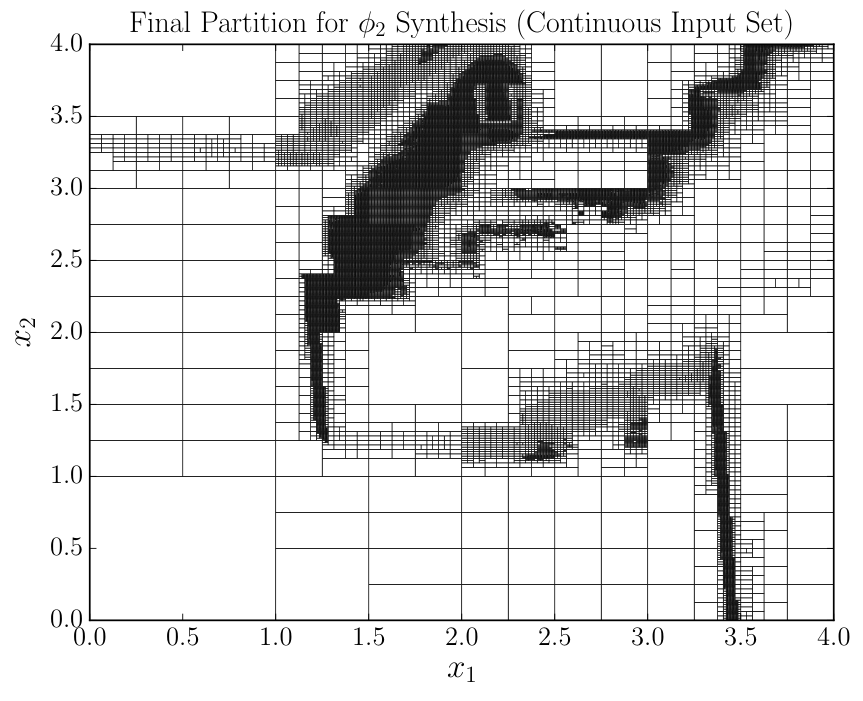
6.3 DISCUSSION
The synthesis algorithms presented in the previous sections successfully designed controllers from both the finite set of inputs and the continuous set of inputs . Moreover, the algorithms conducted synthesis for two different complex specifications that existing tools could not accommodate, and automatically produced a targeted domain refinement for the two cases so as to achieve a higher level of optimality for the computed controllers. We also consider our approach to be an improvement over related synthesis works in terms of scalability; for instance, our finite-mode algorithm is orders of magnitude faster than the technique used for the synthesis case study in [16], which designed a switching policy for a 3-mode 2D linear system with a simple reachability specification over the course of several days.
To further demonstrate the synthesis procedure, in Figure 18 (Top), we display the verification of system (196) against without any available input with respect to a satisfaction threshold of 0.8 from the work in [23], where the initial states in green have a probability of satisfying the specification which is greater than 0.8, the states in red have a probability which is below 0.8, and the states in yellow are undecided at the level of precision of the available partition. In the bottom left, we display the verification of system (196) under the computed switching policy in the finite-mode section, and in the bottom right, we show the verification of system (196) under the computed control policy from the continuous set of inputs. As expected, moving counter-clockwise through the plots, we observe that some red regions of the state-space are converted to green regions.


It is evident that computing controllers from a continuous set of inputs requires a more significant amount of computational effort compared to the finite input case. The largest portion of the continuous-input synthesis algorithm is expended solving the optimization problems for the value iteration step of the procedure, which is the clear scalability bottleneck of our current implementation. Moreover, we notice that the greatest suboptimality factor decreases at a slower rate as a function of refinement steps in the continuous input case than in the finite mode case, which causes a much finer partition of the domain and is the reason for the manual termination in the former example. We explain this phenomenon by observing that the suboptimality factor is more dependent on the abstraction error when using the continuous set of inputs. To see this, consider an optimal input computed for a state of the product CIMC , yielding an interval of satisfaction for this state. Now, consider another input for a small disturbance . Assuming the dynamics of interest are continuous, it follows that the interval of satisfaction under the disturbed input is . Therefore, the suboptimality factor for this state will be at least , which is the size of the satisfaction interval of the considered state under the computed optimal input. Nonetheless, the algorithm still results in overall progress towards the goal optimality across all metrics as it performs more refinement steps.
7 CONCLUSION
In this paper, we developed abstraction-based controller synthesis techniques for stochastic systems with -regular objectives. First, we showed a method to compute switching policies in stochastic systems with a finite number of modes by performing a permanent component search and a reachability maximization task in an abstraction of the dynamics. We proposed a specification-guided domain partition refinement scheme which targets states causing the most uncertainty in the abstraction and discards the system modes that are guaranteed to be suboptimal. We extended these results to stochastic systems with a continuous set of inputs and designed a synthesis method for the specific class of affine-in-input and affine-in-disturbance systems. Finally, we presented a numerical example where controller synthesis is conducted for both finite and continuous input sets on a nonlinear system with complex temporal logic tasks.
Future works will further explore the relationship between original partitions and their refined versions in order to reduce the number of operations performed in the components search and reachability algorithms after each refinement step and consequently improve scalability of our technique. An adaptation of these algorithms to guarantee a monotone decrease of the suboptimality factor throughout the synthesis procedure will also be investigated. Obtaining formal convergence guarantees of the refinement heuristic is another important issue.. Other immediate research directions include the study of wider classes of systems with continuous sets of inputs to which our abstraction-based technique can be extended.
References
- [1] A. Pnueli, The temporal logic of programs, in: 18th Annual Symposium on Foundations of Computer Science (sfcs 1977), IEEE, pp. 46–57.
- [2] W. Thomas, Automata on infinite objects, in: Formal models and semantics, Elsevier, 1990, pp. 133–191.
- [3] P. Tabuada, G. J. Pappas, Linear time logic control of discrete-time linear systems, IEEE Transactions on Automatic Control 51 (12) (2006) 1862–1877.
- [4] M. Kloetzer, C. Belta, A fully automated framework for control of linear systems from temporal logic specifications, IEEE Transactions on Automatic Control 53 (1) (2008) 287–297.
- [5] B. Yordanov, J. Tumova, I. Cerna, J. Barnat, C. Belta, Temporal logic control of discrete-time piecewise affine systems, IEEE Transactions on Automatic Control 57 (6) (2011) 1491–1504.
- [6] M. Rungger, M. Mazo Jr, P. Tabuada, Specification-guided controller synthesis for linear systems and safe linear-time temporal logic, in: Proceedings of the 16th international conference on Hybrid systems: computation and control, ACM, 2013, pp. 333–342.
- [7] M. Rungger, M. Zamani, Scots: A tool for the synthesis of symbolic controllers, in: Proceedings of the 19th international conference on hybrid systems: Computation and control, ACM, 2016, pp. 99–104.
- [8] J. Liu, N. Ozay, Finite abstractions with robustness margins for temporal logic-based control synthesis, Nonlinear Analysis: Hybrid Systems 22 (2016) 1–15.
- [9] S. Sadraddini, C. Belta, Formal synthesis of control strategies for positive monotone systems, IEEE Transactions on Automatic Control 64 (2) (2018) 480–495.
- [10] C. Belta, B. Yordanov, E. A. Gol, Formal methods for discrete-time dynamical systems, Vol. 89, Springer, 2017.
- [11] C. Baier, J.-P. Katoen, K. G. Larsen, Principles of model checking, MIT press, 2008.
- [12] M. L. Bujorianu, J. Lygeros, M. C. Bujorianu, Bisimulation for general stochastic hybrid systems, in: International Workshop on Hybrid Systems: Computation and Control, Springer, 2005, pp. 198–214.
- [13] A. Abate, A. D’Innocenzo, M. D. Di Benedetto, S. S. Sastry, Markov set-chains as abstractions of stochastic hybrid systems, in: International Workshop on Hybrid Systems: Computation and Control, Springer, 2008, pp. 1–15.
- [14] A. Abate, A. D’Innocenzo, M. D. Di Benedetto, Approximate abstractions of stochastic hybrid systems, IEEE Transactions on Automatic Control 56 (11) (2011) 2688–2694.
- [15] M. Kwiatkowska, G. Norman, D. Parker, Prism 4.0: Verification of probabilistic real-time systems, in: International conference on computer aided verification, Springer, 2011, pp. 585–591.
- [16] M. Lahijanian, S. B. Andersson, C. Belta, Formal verification and synthesis for discrete-time stochastic systems, IEEE Transactions on Automatic Control 60 (8) (2015) 2031–2045.
- [17] R. Givan, S. Leach, T. Dean, Bounded-parameter Markov decision processes, Artificial Intelligence 122 (1-2) (2000) 71–109.
- [18] N. Cauchi, L. Laurenti, M. Lahijanian, A. Abate, M. Kwiatkowska, L. Cardelli, Efficiency through Uncertainty: Scalable Formal Synthesis for Stochastic Hybrid Systems, arXiv e-prints (2019) arXiv:1901.01576arXiv:1901.01576.
- [19] N. Cauchi, K. Degiorgio, A. Abate, StocHy: automated verification and synthesis of stochastic processes, arXiv preprint arXiv:1901.10287 (2019).
- [20] K. Y. Rozier, Linear temporal logic symbolic model checking, Computer Science Review 5 (2) (2011) 163–203.
- [21] E. M. Wolff, U. Topcu, R. M. Murray, Robust control of uncertain Markov decision processes with temporal logic specifications, in: Decision and Control (CDC), 2012 IEEE 51st Annual Conference on, IEEE, 2012, pp. 3372–3379.
- [22] E. M. Hahn, V. Hashemi, H. Hermanns, M. Lahijanian, A. Turrini, Interval markov decision processes with multiple objectives: From robust strategies to pareto curves, ACM Transactions on Modeling and Computer Simulation (TOMACS) 29 (4) (2019) 1–31.
- [23] M. Dutreix, S. Coogan, Specification-guided verification and abstraction refinement of mixed monotone stochastic systems, IEEE Transactions on Automatic Control (2020).
- [24] R. Majumdar, K. Mallik, S. Soudjani, Symbolic Controller Synthesis for Büchi Specifications on Stochastic Systems, arXiv e-prints (2019) arXiv:1910.12137arXiv:1910.12137.
- [25] O. Hernández-Lerma, J. B. Lasserre, Discrete-time markov control processes, volume 30 of applications of mathematics, Springer 10 (1996) 978–1.
- [26] M. Dutreix, S. Coogan, Efficient Verification for Stochastic Mixed Monotone Systems, in: International Conference on Cyber-Physical Systems, 2018.
- [27] K. Sen, M. Viswanathan, G. Agha, Model-checking Markov chains in the presence of uncertainties, in: International Conference on Tools and Algorithms for the Construction and Analysis of Systems, Springer, 2006, pp. 394–410.
- [28] S. Haddad, B. Monmege, Interval iteration algorithm for mdps and imdps, Theoretical Computer Science 735 (2018) 111–131.
- [29] J.-P. Katoen, Model checking meets probability: A gentle introduction.
- [30] S. Soudjani, C. Gevaerts, A. Abate, Faust 2: Formal abstractions of uncountable-state stochastic processes, arXiv preprint arXiv:1403.3286 (2014).
- [31] S. Coogan, M. Arcak, Efficient finite abstraction of mixed monotone systems, in: Proceedings of the 18th International Conference on Hybrid Systems: Computation and Control, ACM, 2015, pp. 58–67.
- [32] M. Hirsch, H. Smith, Monotone dynamical systems, Handbook of differential equations: Ordinary differential equations 2 (2005) 239–357.
- [33] D. Wu, X. Koutsoukos, Reachability analysis of uncertain systems using bounded-parameter Markov decision processes, Artificial Intelligence 172 (8-9) (2008) 945–954.
- [34]
PACE, Partnership for an Advanced
Computing Environment (PACE) (2017).
URL http://www.pace.gatech.edu - [35] K. Chatterjee, L. De Alfaro, T. A. Henzinger, Trading memory for randomness, in: First International Conference on the Quantitative Evaluation of Systems, 2004. QEST 2004. Proceedings., IEEE, 2004, pp. 206–217.
Proof of Lemma 1
We provide a constructive proof for this lemma. Consider a product BMDP with set of states , set of policies and set of memoryless policies . We define the greatest permanent accepting BSCC as the set of all states of such that, if , then there exists a policy in such that belongs to a permanent accepting BSCC in .
The first part of the proof consists in showing that there exists a set of memoryless policies such that, under all product IMCs induced by a policy in , all states in belong to a permanent winning component simultaneously and, therefore, .
The second part of the proof shows that, for any other states of which can be made a permanent winning component under some policy in , there exists a set of memoryless policies in (which is a subset of ), such that all these states are a permanent winning component simultaneously.
I] Proof of existence of memoryless policies generating the greatest permanent accepting BSCC as a permanent winning component
First, we constructively show that, if there exists a policy generating a permanent accepting BSCC in , and if there exists another policy generating a permanent accepting BSCC in , then there has to exist a set of memoryless policies in causing the set to be a permanent winning component in . Consider a policy constructed as follows:
1) For the states in , consider the following reasoning: by virtue of being a permanent accepting BSCC for some policy, it has to hold that, for some state , and , for some . Moreover, as is a permanent BSCC under , for any state , there exists a sequence of inputs chosen by such that the lower bound probability of reaching is 1, that is, . Since reachability problems in BMDPs have memoryless optimal policies [28], it must be true that a memoryless policy choosing no other actions than the ones prescribed by at all states and guaranteeing for all exists as well. For all , set .
2) For all states , apply the same reasoning with respect to the problem of reaching instead of , that is, there exists a memoryless policy choosing no other actions than the ones prescribed by such that for all . For all , set .
3) For all states , choose any action in as .
As is a permanent BSCC under , no state of can transition outside of under , that is, it holds that . Moreover, since for all , it follows that any trajectory starting in will always return to , that is, for all , and will additionally never reach a state satisfying . Therefore, any trajectory starting in satisfies the Rabin acceptance condition with lower bound probability 1, and is a member of the permanent winning component of . Furthermore, for all , we have and thus, is a member of the permanent winning component of . Therefore, is a member of the permanent winning component of .
Iteratively applying this logic with and any other member of shows that there exists a set of policies in such that all states in belong to a permanent winning component simultaneously.
II] Proof of existence of greatest permanent winning component and of memoryless policies generating this component
Now, we consider the set of all states of which do not belong to .
We define the set of all policies which are history-dependent outside of and generate with an (arbitrary) memoryless policy on the states in .
For a policy , the set of all states that belong to the permanent winning component of without being a member of — that is, and — has to satisfy two conditions:
a) does not allow a transition outside of under any adversary of , that is, for all ,
b) No subset of can form a losing component under any adversary of , that is, no state in is a member of the largest losing component of the product IMC , or .
With these two conditions fulfilled, all states in either transition to or reach an accepting BSCC formed within under all adversaries of , and therefore reach an accepting BSCC with lower bound probability 1.
Now, we constructively show that, if there exists a policy inducing a product IMC with permanent winning component and with a set of states satisfying conditions a) and b) such that and , and if there exists a policy inducing a product IMC with permanent winning component and with a set of states satisfying conditions a) and b) such that and , then there has to exist a memoryless policy inducing a product IMC with permanent winning component and with the set of states satisfying conditions a) and b) such that . Consider a policy constructed as follows:
1) For all state , consider the following reasoning inspired by the arguments in the proof of [35, Theorem 8] on the optimality of memoryless policies in MDPs for Rabin objectives: for any state in , it must be true that any trajectory initiated at under policy reaches with lower bound probability 1 a set such that the continuation of any trajectory that reaches is confined to and either reaches or visits an unmatched accepting Rabin state in infinitely often. Consider the arbitrarily ordered set of all such sets which can by reached by some initial state under . Due to the optimality of memoryless policies for reachability problems in BMDPs and the properties of the sets, there must exist a memoryless policy such that, for all , , where is the set of all unmatched Rabin accepting states in , and . Set for all . Apply the same procedure recursively to and replacing with , then to etc. For the states outside the sets, design such that , which again can be achieved with a memoryless choice of actions due to the optimality of memoryless policies for reachability and the fact that satisfies this condition.
2) For all state , choose the actions in by following the same reasoning as in 1) after replacing with and with .
3) For all state (not in , since actions are already fixed in this set), choose any action in as .
By construction, the set satisfy condition a) and b), as no subset of can form a losing component under the actions prescribed by and no trajectory can leave . Therefore, is a subset of the permanent winning component of .
Replacing the set from the beginning of section II] with and applying the same process iteratively proves the existence of a set satisfying the properties enunciated in the lemma and of a set of memoryless policies generating .