VerSe: A Vertebrae Labelling and Segmentation Benchmark
for Multi-detector CT Images

Anjany Sekuboyina Email: anjany.sekuboyina@tum.de Address: Department of Informatics, Technical University of Munich, Germany. Address: Munich School of BioEngineering, Technical University of Munich, Germany. Address: Department of Neuroradiology, Klinikum Rechts der Isar, Germany. Malek E. Husseini Address: Department of Informatics, Technical University of Munich, Germany. Address: Department of Neuroradiology, Klinikum Rechts der Isar, Germany. Amirhossein Bayat Address: Department of Informatics, Technical University of Munich, Germany. Address: Department of Neuroradiology, Klinikum Rechts der Isar, Germany. Maximilian Löffler Address: Department of Neuroradiology, Klinikum Rechts der Isar, Germany. Hans Liebl Address: Department of Neuroradiology, Klinikum Rechts der Isar, Germany. Hongwei Li Address: Department of Informatics, Technical University of Munich, Germany. Giles Tetteh Address: Department of Informatics, Technical University of Munich, Germany. Jan Kukačka Address: Institute of Biological and Medical Imaging, Helmholtz Zentrum München, Germany Christian Payer Address: Institute of Computer Graphics and Vision, Graz University of Technology, Austria Darko Štern Address: Gottfried Schatz Research Center: Biophysics, Medical University of Graz, Austria Martin Urschler Address: School of Computer Science, The University of Auckland, New Zealand Maodong Chen Address: Computer Vision Group, iFLYTEK Research South China, China Dalong Cheng Address: Computer Vision Group, iFLYTEK Research South China, China Nikolas Lessmann Address: Department of Radiology and Nuclear Medicine, Radboud University Medical Center Nijmegen, The Netherlands Yujin Hu Address: Shenzhen Research Institute of Big Data, China Tianfu Wang Address: School of Biomedical Engineering, Health Science Center, Shenzhen University, China Dong Yang Address: NVIDIA Corporation, USA Daguang Xu Address: NVIDIA Corporation, USA Felix Ambellan Address: Zuse Institute Berlin, Germany Tamaz Amiranashvili Address: Zuse Institute Berlin, Germany Moritz Ehlke Address: 1000shapes GmbH, Berlin, Germany Hans Lamecker Address: 1000shapes GmbH, Berlin, Germany Sebastian Lehnert Address: 1000shapes GmbH, Berlin, Germany Marilia Lirio Address: 1000shapes GmbH, Berlin, Germany Nicolás Pérez de Olaguer Address: 1000shapes GmbH, Berlin, Germany Heiko Ramm Address: 1000shapes GmbH, Berlin, Germany Manish Sahu Address: Zuse Institute Berlin, Germany Alexander Tack Address: Zuse Institute Berlin, Germany Stefan Zachow Address: Zuse Institute Berlin, Germany Tao Jiang Address: Damo Academy, Alibaba Group, China Xinjun Ma Address: Damo Academy, Alibaba Group, China Christoph Angerman Address: Department of Mathematics, University of Innsbruck, Austria Xin Wang Address: Department of Electronic Engineering, Fudan University, China Kevin Brown Address: New York University, USA Alexandre Kirszenberg Address: EPITA Research and Development Laboratory (LRDE), France Élodie Puybareau Address: EPITA Research and Development Laboratory (LRDE), France Di Chen Address: Deep Reasoning AI Inc, USA Yiwei Bai Address: Deep Reasoning AI Inc, USA Brandon H. Rapazzo Address: Deep Reasoning AI Inc, USA Timyoas Yeah Address: Chinese Academy of Sciences, China Amber Zhang Address: Technical University of Munich, Germany Shangliang Xu Address: East China Normal University Feng Hou Address: Institute of Computing Technology, Chinese Academy of Sciences, China Address: Lenovo Group, China Zhiqiang He Chan Zeng Address: Ping An Technologies, China Zheng Xiangshang Address: College of Computer Science and Technology, Zhejiang University, China Address: Real Doctor AI Research Centre, Zhejiang University, China Xu Liming Address: College of Computer Science and Technology, Zhejiang University, China Tucker J. Netherton Address: The University of Texas MD Anderson Cancer Center, USA Raymond P. Mumme Address: The University of Texas MD Anderson Cancer Center, USA Laurence E. Court Address: The University of Texas MD Anderson Cancer Center, USA Zixun Huang Address: Department of Electronic and Information Engineering, The Hong Kong Polytechnic University, China Chenhang He Address: Department of Computing, The Hong Kong Polytechnic University, China Li-Wen Wang Address: Department of Electronic and Information Engineering, The Hong Kong Polytechnic University, China Sai Ho Ling Address: The School of Biomedical Engineering, University of Technology Sydney, Australia Lê Duy Huỳnh Address: EPITA Research and Development Laboratory (LRDE), France Nicolas Boutry Address: EPITA Research and Development Laboratory (LRDE), France Roman Jakubicek Address: Department of Biomedical Engineering, Brno University of Technology, Czech Republic Jiri Chmelik Address: Department of Biomedical Engineering, Brno University of Technology, Czech Republic Supriti Mulay Address: Indian Institute of Technology Madras, India Address: Healthcare Technology Innovation Centre, India Mohanasankar Sivaprakasam Address: Indian Institute of Technology Madras, India Address: Healthcare Technology Innovation Centre, India Johannes C. Paetzold Address: Department of Informatics, Technical University of Munich, Germany. Suprosanna Shit Address: Department of Informatics, Technical University of Munich, Germany. Ivan Ezhov Address: Department of Informatics, Technical University of Munich, Germany. Benedikt Wiestler Address: Department of Neuroradiology, Klinikum Rechts der Isar, Germany. Ben Glocker Address: Department of Computing, Imperial College London, UK Alexander Valentinitsch Address: Department of Neuroradiology, Klinikum Rechts der Isar, Germany. Markus Rempfler Address: Friedrich Miescher Institute for Biomedical Engineering, Switzerland Björn H. Menze Note: BM and JSK are supervising authors Address: Department of Informatics, Technical University of Munich, Germany. Address: Department for Quantitative Biomedicine, University of Zurich, Switzerland. Jan S. Kirschke Note: BM and JSK are supervising authors Address: Department of Neuroradiology, Klinikum Rechts der Isar, Germany.

Abstract

Vertebral labelling and segmentation are two fundamental tasks in an automated spine processing pipeline. Reliable and accurate processing of spine images is expected to benefit clinical decision support systems for diagnosis, surgery planning, and population-based analysis of spine and bone health. However, designing automated algorithms for spine processing is challenging predominantly due to considerable variations in anatomy and acquisition protocols and due to a severe shortage of publicly available data. Addressing these limitations, the Large Scale Vertebrae Segmentation Challenge (VerSe) was organised in conjunction with the International Conference on Medical Image Computing and Computer Assisted Intervention (MICCAI) in 2019 and 2020, with a call for algorithms tackling the labelling and segmentation of vertebrae. Two datasets containing a total of 374 multi-detector CT scans from 355 patients were prepared and 4505 vertebrae have individually been annotated at voxel level by a human-machine hybrid algorithm (https://osf.io/nqjyw/, https://osf.io/t98fz/). A total of 25 algorithms were benchmarked on these datasets. In this work, we present the results of this evaluation and further investigate the performance variation at the vertebra level, scan level, and different fields of view. We also evaluate the generalisability of the approaches to an implicit domain shift in data by evaluating the top-performing algorithms of one challenge iteration on data from the other iteration. The principal takeaway from VerSe: the performance of an algorithm in labelling and segmenting a spine scan hinges on its ability to correctly identify vertebrae in cases of rare anatomical variations. The VerSe content and code can be accessed at: https://github.com/anjany/verse.

\newpageafter

author

1 Introduction

The spine is an important part of the musculoskeletal system, sustaining and supporting the body and its organ structure while playing a major role in our mobility and load transfer. It also shields the spinal cord from injuries and mechanical shocks due to impacts. Efforts towards quantification and understanding of the biomechanics of the human spine include quantitative imaging (Löffler et al. 2020a), finite element modelling (FEM) of the vertebrae (Anitha et al. 2020), alignment analysis (Laouissat et al. 2018) of the spine and complex biomechanical models (Oxland 2016). Biomechanical alterations can cause severe pain and disability in the short term, and can demonstrate worse consequences in the long term, e.g. osteoporosis leads to an 8-fold higher mortality rate (Cauley et al. 2000). In spite of their criticality, spinal pathologies are often under-diagnosed (Howlett et al. 2020; Müller et al. 2008; Williams et al. 2009). This calls for computer-aided assistance for efficient and early detection of such pathologies, enabling prevention or effective treatment.

Vertebral labelling and vertebral segmentation are two fundamental tasks in understanding spine image data. Labelled and segmented spines have diagnostic implications for detecting and grading vertebral fractures, estimating the spinal curve, and recognising spinal deformities such as scoliosis and kyphosis. From a non-diagnostic perspective, these tasks enable efficient biomechanical modelling, FEM analysis, and surgical planning for metal insertions. Vertebral labelling can be performed quickly by a medical expert, on smaller datasets, as it follows clear rules (Wigh 1980). But, manually segmenting them is unfeasible owing to the time required for annotating large structures (e.g. 25 objects of interest with a size of $\sim 10^{4}$ voxels each). Moreover, the complex morphology of the vertebra’s posterior elements combined with lower scan resolutions prevents a consistent and accurate manual delineation. Automating these tasks also involves multiple challenges: highly varying fields of view (FoV) across datasets (unlike brain images), large scan sizes, highly correlating shapes of adjacent vertebrae, scan noise, different scanner settings, and multiple anomalies or pathologies being present. For example, the presence of vertebral fractures, metal implants, cement, or transitional vertebrae should be considered during algorithm design. Fig. 1 illustrates this diversity using the scans included in the Large Scale Vertebrae Segmentation Challenge (VerSe).

1.1 Terminology

In this section, we introduce three spine-processing terms frequently used in this work: localisation, labelling, segmentation. As used in the rest of the work: Localisation is the task of detecting a 3D coordinate on the vertebra and labelling is the task of detecting a 3D coordinate on the vertebra as well as identifying the vertebrae. Specifically, labelling superscribes localisation by assigning a 3D coordinate as well as a class to the vertebra (C1-C6, T1-T13, L1-L5, as well as T13 and L6). Unless mentioned otherwise, spine segmentation is a voxel-level, multi-class annotation problem, where in each vertebra level has a defined class label (e.g. C1 $\rightarrow$ 1, C2 $\rightarrow$ 2, T1 $\rightarrow$ 8 etc.). It can now be seen that once a vertebra is segmented, its labelling and localisation is implied.

1.2 Prior Work

Spine image analysis has received subsistence attention from the medical imaging community over the years. Although computed tomography (CT) is a preferred modality for studying the ‘bone’ part of a spine due to high bone-to-soft-tissue contrast, there are several prior works on the tasks of labelling and segmenting the spine using multiple modalities in addition to CT such as magnetic resonance imaging (MRI), and 2D radiographs. There are works tackling segmentation (most of which inherently include vertebral labelling), and those tackling labelling specifically from a landmark-detection perspective.

1.2.1 Vertebral Segmentation

Traditionally, vertebral segmentation was performed using model-based approaches, which loosely involve fitting a shape prior to the spine and deforming it so that it fits the given spine. The incorporated shape priors range from geometric models (Štern et al. 2011; Ibragimov et al. 2014; Ibragimov et al. 2017), deformed with Markov random fields (MRF) (Kadoury et al. 2011; Kadoury et al. 2013), statistical shape models (Rasoulian et al. 2013; Pereañez et al. 2015; Castro-Mateos et al. 2015), and active contours (Leventon et al. 2002; Athertya & Kumar 2016). There are also intensity-based approaches such as level sets (Lim et al. 2014) and a priori variational intensity models (Hammernik et al. 2015). Landmark frameworks tackling fully automated vertebral labelling and segmentation from a shape-modelling perspective exist (Klinder et al. 2009; Korez et al. 2015).

With the increased adoption of machine learning in image analysis, works incorporating significant data-based learning components have been proposed. Suzani et al. 2015a propose using a multi-layer perceptron (MLP) to detect the vertebral bodies and employ deformable registration for segmentation. Similar in philosophy, Chu et al. 2015 propose random forest regression for locating and identifying the vertebrae followed by segmentation performed using random forest classification at a voxel level. Incorporating deep learning, Korez et al. 2016 learn vertebral appearances using 3D convolutional neural networks (CNN) and predict probability maps, which are then used to guide the boundaries of a deformable vertebral model.

The recent advent of deep learning in image analysis and increased computing capabilities have led to works wherein deformable shape modelling and/or vertebral identification was replaced by data-driven learning of the vertebral shape using deep neural networks. Sekuboyina et al. 2017a perform a patch-based binary segmentation of the spine using a U-Net (Ronneberger et al. 2015) (or a fully convolutional network, FCN) followed by denoising the spine mask using a low-resolution heat map. Sekuboyina et al. 2017b propose two neural networks for vertebral segmentation in the lumbar region. First, an MLP learns to regress the localisation of the lumbar region, following which a U-Net performs multi-class segmentation. Improving on this, Janssens et al. 2018 replace the MLP with a CNN, thus performing multi-class segmentation of lumbar vertebrae with two successive CNNs. Lessmann et al. 2018 propose a two-staged iterative approach, wherein the first stage involves identifying and segmenting one vertebra after another at a lower resolution, followed by a second CNN to refine the lower-resolution masks. Building on this, Lessmann et al. 2019 proposed a single-stage FCN which iteratively regresses the vertebrae’s anatomical label and segments it. Once the entire scan is segmented, the vertebral labels are adjusted using a maximum likelihood approach. Approaching the problem from the other end, Payer et al. 2020 propose a coarse-to-fine approach involving three stages, spine localisation, vertebra labelling, and vertebrae segmentation, all three utilising purposefully designed FCNs. Note that (Payer et al. 2020) and (Lessmann et al. 2019) are included in this VerSe benchmark.

1.2.2 Vertebral Labelling

Similar to the segmentation works discussed above, classical works on vertebral labelling also involve deformable shape or pose models (Ibragimov et al. 2015; Cai et al. 2015). Learning from data, Major et al. 2013 landmark point using probabilistic boosting trees followed by matching local models using MRFs. As such, works transitioned towards incorporating machine learning using hand-crafted features. Glocker et al. 2012; Glocker et al. 2013 employ context features to regress vertebral centroids using regression forests and MRFs. Bromiley et al. 2016 use Haar-like features to identify vertebrae using random forest regression voting. Similarly, Suzani et al. 2015b employ an MLP to regress the centroid locations. With the incorporation of the ubiquitous CNNs, Chen et al. 2015 proposed a joint-CNN as a combination of random forests for candidate selection followed by a CNN for identifying the vertebrae. Forsberg et al. 2017 employ CNNs to detect the vertebrae followed by labelling them using graphical models.

Going fully convolutional and regressing on input-sized heatmap responses instead of directly learning the centroid locations (which is a highly non-linear mapping), Yang et al. 2017a; Yang et al. 2017b propose DI2IN, an FCN, for heatmap regression of the vertebral centroids at lower resolution, followed by correction using message passing and recurrent neural networks (RNN) respectively. Utilising a single network termed Btrfly-Net, Sekuboyina et al. 2018; Sekuboyina et al. 2020 propose labelling sagittal and coronal maximum intensity projections (MIP) of the spine, reinforced by a prior learnt using a generative adversarial network. Using a three-staged approach, Liao et al. 2018 combine a CNN with a bidirectional-RNN to label and then fine-tune network predictions. Handling close to two hundred landmarks, Mader et al. 2019 use multistage, 3D CNNs to regress heatmaps followed by fine-tuning using regression trees regularised by conditional random fields. Payer et al. 2019 propose a two-stream architecture called spatial-configuration net for integrating global context and local detail in one end-to-end trainable network. With a similar motivation of combining long-range and short-range contextual information, Chen et al. 2019 propose combining a 3D localising network with a 2D labelling network.

Refer to caption — Figure 1: Example scan slices from the VerSe datasets, labelled clockwise. In addition to the wide variation in the fields of view, we illustrate with fractured vertebrae (B, J), metal insertions (C), cemented vertebrae (G), transitional vertebrae (L6 and T13 in D and I respectively), and a noisy scan (K).

Dataset	#train	#test	Annotations
CSI-Seg 2014 (Yao et al. 2012)	10	10	S
CSI-Label 2014 (Glocker et al. 2012)	242	60	L
Dataset-5 (Ibragimov et al. 2014)	10	–	S (Lumbar)
xVertSeg 2016 (Korez et al. 2015)	15	10	S (Lumbar)
VerSe 2019	80	80	L + S
VerSe 2020	103	216	L + S

Table 1: Comparing VerSe with other publicly available, annotated CT datasets. In ‘Annotations’, L and S refer to annotations concerning the labelling (3D centroid coordinates) and segmentation tasks (voxel-level labels), respectively.

1.3 Motivation

Recent spine-processing approaches discussed above are predominantly data-driven, thus requiring annotated data to either learn from (e.g. neural network weights) or to tune and adapt parameters (e.g. active shape model parameters). In spite of this, publicly available data with good-quality annotations is scarce. Eventually, the algorithms are either insufficiently validated or validated in private datasets, preventing a fair comparison. SpineWeb¹¹ 1 spineweb.digitalimaginggroup.ca, an archive for multi-modal spine data, lists a total of four CT datasets with voxel-level or vertebra level annotations: CSI2014-Seg (Yao et al. 2012; Yao et al. 2016), xVertSeg (Korez et al. 2015), Dataset-5 (Ibragimov et al. 2014), and CSI2014-Label (Glocker et al. 2012). Table 1 provides an overview of these public datasets. Except Dataset-5, all datasets were released as part of segmentation and labelling challenges organised as part of the computational spine imaging (CSI) workshop at MICCAI. CSI2014-Seg and Label were made publicly available in conjunction with MICCAI 2014 and xVertSeg with MICCAI 2016. Credit is due to these incipient steps towards open-sourcing data, which have yielded interest in spine processing. A significant portion of the work detailed in Sec. 1.2 is benchmarked on these datasets. However, much is to be desired in terms of data size and data variability. The largest spine CT dataset with voxel-level annotations to date consists of 25 scans, with lumbar annotations only. CSI-Label, even though it is a collection of 302 scans with high data variability, is collected from a single centre (Department of Radiology, University of Washington), possibly inducing a bias.

With the objective of addressing the need for a large spine CT dataset and to provide a common benchmark for current and future spine-processing algorithms, we prepared a dataset of 374 multi-detector, spine CT (MDCT) scans (an order of magnitude ( $\sim$ 20 times) increase from the prior datasets) with vertebral-level (3D centroids) and voxel-level annotations (segmentation masks). This dataset was made publicly available as part of the Large Scale Vertebrae Segmentation challenge (VerSe), organised in conjunction with MICCAI 2019 and 2020. In total, 160 scans were released as part of VerSe‘19 and 355 scans for VerSe‘20, with a call for fully automated and interactive algorithms for the tasks of vertebral labelling and vertebral segmentation.

As part of the VerSe challenge, we evaluated twenty-five algorithms (eleven for VerSe‘19, thirteen for VerSe‘20, and one baseline). This work presents an in-depth analysis of this benchmarking process, in addition to the technical aspects of the challenge. In summary, the contribution of this work includes:

•

A brief description of the setup for the VerSe‘19 and VerSe‘20 challenges (Sec. 2)
•

A summary of the three top-performing algorithms from each iteration of VerSe, along with a description of the in-house, interactive spine processing algorithm utilised to generate the initial annotation. (Sec. 3)
•

Performance overview of the participating algorithms and further experimentation provide additional insights into the algorithms. (Sec. 4)

2 Materials and challenge setup

2.1 Data and annotations

The entire VerSe dataset consists of 374 CT scans made publicly available after anonymising (including defacing) and obtaining an ethics approval from the institutional review board for the intended use. The data was collected from 355 patients with a mean age of $\sim 59(\pm 17)$ years. The data is multi-site and was acquired using multiple CT scanners, including the four major manufacturers (GE, Siemens, Phillips and Toshiba). Care was taken to compose the data to resemble a typical clinical distribution in terms of FoV, scan settings, and findings. For example, it consists of a variety of FoVs (including cervical, thoraco-lumbar and cervico-thoraco-lumbar scans), a mix of sagittal and isotropic reformations, and cases with vertebral fractures, metallic implants, and foreign materials. Fig. 1 illustrates this variability in the VerSe dataset. Refer to Löffler et al. 2020b; Liebl et al. 2021 for further details on the data composition.

The dataset consists of two types of annotations: 1) 3D coordinate locations of the vertebral centroids and 2) voxel-level labels as segmentation masks. Twenty-six vertebrae (C1 to L5, and the transitional T13 and L6) were considered for annotation with labels from 1 to 24, along with labels 25 and 28 for L6 and T13, respectively. Note that partially visible vertebrae at the top or bottom of the scan (or both) were not annotated. Annotations were generated using a human-hybrid approach. The initial centroids and segmentation masks were generated by an automated algorithm (details in Sec. 3) and were manually and iteratively refined. Initial refinement was performed by five trained medical students followed by further refinement, rejection, or acceptance by three trained radiologists with a combined experience of 30 years (ML, HL, and JSK). All annotations were finally approved by one radiologist with 19 years of experience in spine imaging (JSK).

2.2 Challenge setup

VerSe was organised in two iterations, first at MICCAI 2019 and then at MICCAI 2020 with a call for algorithms tackling vertebral labelling and segmentation. Both the iterations followed an identical setup, wherein the challenge consisted of three phases: one training and two test phases. In the training stage, participants have access to the scans and their annotations, on which they can propose and train their algorithms. In the first test phase, termed Public in this work, participants had access to the test scans on which they were supposed to submit the predictions. In the second test phase, termed Hidden, participants had no access to any test scans but were requested to submit their code in a docker container. The dockers were evaluated on hidden test data, thus disabling re-training on test data or fine-tuning via over-fitting. Information about the data and its split across the two VerSe iterations is tabulated in Table 2. All the 374 scans of VerSe dataset and their annotations are now publicly available, 2019: https://osf.io/nqjyw/ and 2020: https://osf.io/t98fz/. We have also open-sourced the data processing and the evaluation scripts. All VerSe-content is accessible at https://github.com/anjany/verse

VerSe	Patients	Scans	Scan split	Vertebrae (Cer/Tho/Lum)
2019	141	160	80/40/40	1725 (220/884/621)
2020	300	319	113/103/103	4141 (581/2255/1305)
Total	355	374	141/120/113	4505 (611/2387/1507)

Table 2: Data split and additional details concerning the two iterations of VerSe. Scan split indicates the split of the data into training/Public test/Hidden test phases. Cer, Tho, and Lum refer to the number of vertebrae from the cervical, thoracic, and lumbar regions, respectively. Note that of the 300 patients in VerSe‘20, 86 patients are from VerSe‘19, resulting in the total patients not being an ad hoc sum of the two iterations. VerSe‘19 data can be identified by its image ID being less than 500. (Overlap is not absolute owing to the difference in the objectives of the two challenge iterations.)

2.3 Evaluation metrics

In this work, we employ four metrics for evaluation, two for the task of labelling and two for the task of segmentation. Note that the evaluation protocol employed for ranking the challenge participants builds on the one presented in this work. Please refer to A for an overview of the former.

Labelling. To evaluate the labelling performance, we compute the Identification Rate ( $id.rate$ ) and localisation distance ( $d_{\text{mean}}$ ): Assuming a given scan contains $N$ annotated vertebrae and denoting the true location of the $i^{th}$ vertebra with $x_{i}$ and it predicted location with $\hat{x}_{i}$ , the vertebra $i$ is correctly identified if $\hat{x}_{i}$ is the closest landmark predicted to $x_{i}$ among $\{x_{j}\forall j\mathrm{\penalty\ in\penalty\ }1,2,...,N\}$ and the Euclidean distance between the ground truth and the prediction is less than $20\,\mathrm{mm}$ , i.e. $||\hat{x}_{i}-x_{i}||_{2}<$ $20\,\mathrm{mm}$ . For a given scan, $id.rate$ is then defined as the ratio of the correctly identified vertebrae to the total vertebrae present in the scan. Similarly, the localisation distance is computed as $d_{\text{mean}}=(\sum_{i=1}^{N}||\hat{x}_{i}-x_{i}||_{2})/N$ , the mean of the euclidean distances between the ground truth vertebral locations and their predictions, per scan. Typically, we report the mean measure over all the scans in the dataset. Note that our evaluation of the labelling tasks slightly deviates from its definition in (Glocker et al. 2012), where $id.rate$ and $d_{\text{mean}}$ are computed not at scan-level but at dataset level.

Segmentation. To evaluate the segmentation task, we choose the ubiquitous Dice coefficient (Dice) and Hausdorff distance ( $HD$ ). Denoting the ground truth by $T$ and the algorithmic predictions by $P$ , and indexing the vertebrae with $i$ , we compute the mean Dice score across the vertebrae as follows:

\text{Dice}(P,T)=\frac{1}{N}\sum_{i=1}^{N}\frac{2|P_{i}\cap T_{i}|}{|P_{i}|+|T_{i}|}.

(1)

As a surface measure, we compute the mean Hausdorff distance over all vertebrae as:

HD(P,T)=\frac{1}{N}\sum_{i=1}^{N}\max\left\{\sup\limits_{p\in\mathcal{P}_{i}}\inf\limits_{t\in\mathcal{T}_{i}}d(p,t),\sup\limits_{t\in\mathcal{T}_{i}}\inf\limits_{p\in\mathcal{P}_{i}}d(p,t)\right\},

(2)

where $\mathcal{P}_{i}$ and $\mathcal{T}_{i}$ denote the surfaces extracted from the voxel masks of the $i^{\text{th}}$ vertebra and $d(p,t)=||p-t||_{2}$ , i.e a Euclidean distance between the points $p$ and $t$ on the two surfaces.

Outliers. In multi-class labelling and segmentation, there will be cases where the prediction of an algorithm will contain fewer vertebrae than the ground truth. In such cases, $d_{\text{mean}}$ and $HD$ are not defined for the missing vertebrae. For the sake of analysis in this work, we ignore such vertebrae while computing the averages. This way, we still get a picture of the algorithm’s performance on the rest of the correctly predicted vertebrae. The missing vertebrae are anyway clearly penalised by the other two metrics, viz. $id.rate$ and Dice.

3 Methods

In this section, we present Anduin, our spine processing framework that enabled the medical experts to generate voxel-level annotations at scale. Then, we present details of select participating algorithms.

3.1 Anduin: Semi-automated spine processing framework

Anduin is a semi-automated, interactive processing tool developed in-house, which was employed to generate the initial annotations for more than 4000 vertebrae. It is a three-staged pipeline consisting of: 1) Spine detection, performed by a light-weight, FCN predicting a low-resolution heatmap over the spine location, 2) Vertebra labelling, based on the Btrfly Net (Sekuboyina et al. 2018) architecture working on sagittal and coronal MIPs of the localised spine region, and finally, 3) Vertebral segmentation, performed by an improved U-Net (Ronneberger et al. 2015; Roy et al. 2018) to segment vertebral patches, extracted at 1mm resolution, around the centroids predicted by the preceding stage. Fig. 2 gives a schematic of the entire framework. Importantly, the detection and labelling stages offer interaction, wherein the user can alter the bounding box predicted during spine detection as well as the vertebral centroids predicted by the labelling stage. Such human-in-loop design enabled the collection of accurate annotations with minimal human effort. We made a web-version of Anduin publicly available to the research community that can be accessed at anduin.bonescreen.de. Refer to B for further details on Anduin (at the time of this work) such as network architecture, training scheme, and post-processing steps. Furthermore, without human-interaction, Anduin is fully automated. We include this version of Anduin in the benchmarking process as ‘Sekuboyina A.’. We note that since the ground-truth segmentation masks are generated with Anduin-predictions as initialisation, there exists a bias. However, the bias is not as strong for the labelling task as the centroid annotations are sparse and have a high intra- and inter-rater variability.

Team / Ref. Author

Method Features

VerSe‘19

zib / Amiranashvili T.

Multi-stage, shape-based approach. Multi-label segmentation with arbitrary labels for vertebrae. Unique label

assignment for based on shape templates. Landmark positions are derived as centres of fitted model.

christoph / Angermann C.

Single-staged, slice-wise approach. One 2.5D U-Net (Angermann et al. 2019) and two 2D U-Nets are employed.

The first network generates 2D projections containing 3D information. Then, one 2D U-Net segments the

projections, one segments the 2D slices. Labels are obtained as centroids of segmentations.

brown / Brown K.

A 3D bounding box around the vertebra is predicted by regressing on a set of canonical landmarks. Each

vertebra is segmented using a residual U-Net and labelled by registering to a common atlas.

iflytek / Chen M.

A three-staged approach. Spine localisation and multi-label segmentation are based on a 3D U-Net. Using the

predicted segmentation mask, the third stage employs a RCNN-based architecture to label the vertebrae.

yangd05 / Dong Y.

Single-staged approach. A 3D U-Net based on neural-architecture search is employed to segment vertebrae as

26-class problem. Vertebral-body centre are located using iterative morphological erosion.

huyujin / Hu Y.

Single-staged, patch-based approach. Based on the nnU-Net (Isensee et al. 2019). All three networks are used:

a 3D-UNet at high resolution, a 3D U-Net at low resolution, and a 2D U-Net.

alibabadamo / Jiang T.

Single-staged approach, employing a V-Net (Milletari et al. 2016) backbone with two heads, one for binary-

segmentation and the other for vertebral-labelling. Vertebrae C2, C7, T12, and L5 are identified and the rest

are inferred from these.

lrde / Kirszenberg A.

Multi-stage, shape-based approach. A combination of three 2D U-Nets generate 3D binary mask of spine.

Anchor points on a skeleton obtained from this mask are used for template matching. Five vertebrae are

chosen for matching, and one with highest score is chosen as a match.

diag / Lessmann N.

Single-staged, patch-based approach. A 3D U-Net (Lessmann et al. 2019) iteratively identifies and segments

the bottom-most visible vertebra in extracted patches, eventually crawling the spine. An additional network is

trained to detect first cervical and thoracic vertebrae.

christian_payer / Payer C.

Multi-staged, patch-wise approach. A 3D U-Net regresses a heatmap of the spinal centre line. Individual vert-

ebrae are localized and are identified with the SpatialConfig-Net (Payer et al. 2020). Each vertebra is then

independently segmented as a binary segmentation.

init / Wang X.

Multi-staged-approach. A single-shot 2D detector is utilised to localise the spine. A modified Btrfly-Net

(Sekuboyina et al. 2018) and a 3D U-Net are employed to address labelling and segmentation respectively.

VerSe‘20

deepreasoningai_team1

/ Chen D.

Multi-staged, patch-based approach. A 3D U-Net coarsely localises the spine. Then, a U-Net performs binary

segmentation, patchwise. Lastly, a 3D Resnet-model identifies the vertebral class taking the vertebral mask

and CT-image segmented vertebra.

carpediem / Hou F.

Multi-staged approach. First, the spine position is located with 3D U-Net. Second the vertebrae are labelled

in the cropped patches. Lastly, U-Net segments individual vertebrae from background using centroids labels.

poly / Huang Z.

Single-staged, patch-based approach. A U-Net with feature-aggregation and squeeze & exictation module is

proposed.Contains two task-specific heads, one for vertebrae labelling and the other for segmentation.

lrde / Huỳnh L. D.

A single model with two-stages, a Mask-RCNN-inspired model incorporating RetinaNet is proposed. First

stage detects and classifies vertebral RoIs. Second stage outputs a binary segmentation for each of the RoIs.

ubmi / Jakubicek R.

Multi-staged, semi-automated approach (Jakubicek et al. 2020). Stages include: spine-canal tracking,

localising and labelling the inter-vertebral disks, and then labelling the vertebrae. Segmentation is based on

graph-cuts.

htic / Mulay S.

Single-staged approach. A 2D Mask R-CNN withcomplete IoU loss performs slice-wise segmentation.

superpod / Netherton T. J.

Multi-staged approach. Combines a 2D FCN for coarse spinal canal segmentation, a multi-view X-Net

(Netherton et al. 2020) for labelling, and a U-Net++ architecture for vertebral segmentation.

rigg / Paetzold J.

A naive 2D U-Net performs multi-class segmentation of sagittal slices.

christian_payer / Payer C.

Similar to Payer C.’s 2019 submission. Different from it, Markov Random fields are employed for post-

processing the localisation stage’s output. Additionally, appropriate floating-point optimisation of network

weights scans into patches.

fakereal / Xiangshang Z.

Both tasks are handled individually. A modified Btrfly-Net (Sekuboyina et al. 2018) detects vertebral key

points. An nnU-Net (Isensee et al. 2019) performs multi-class segmentation.

sitp / Yeah T.

Two-staged approach containing two 3D U-Nets. First one performs coarse localisation of the spine

at low-resolution. Second one performs multi-class segmentation of the vertebra at a higher resolution.

aply / Zeng C.

Multi-staged approach. First stage detects five key-points on the spine using a HRNet. Second,

improved Spatialconfig-Net (Payer et al. 2019) performs the labelling. Segmentation is now a binary problem.

jdlu / Zhang A.

A four-step approach. A patch-based V-Net is used to regress the spine center-line. A key-point localization V-

Net predicts potential vertebral candidates. A three-class vertebrae segmentation network obtains main class of

each vertebrae. Final labels are obtained using a rule-based postprocessing.

Table 3: Brief summary of the participating methods in VerSe benchmark, ordered alphabetically according to referring author.

3.2 Participating methods

Over its two iterations, VerSe has received more than five hundred data download requests. Forty teams uploaded their submissions onto the leaderboards. Of these, eleven and thirteen teams were evaluated for VerSe‘19 and VerSe‘20, respectively. Table 3 provides a brief synopsis of all the participating teams. Below, we present the algorithms proposed by the best and the second-best-performing teams in each iteration of the challenge. C provides the details of the remaining algorithms.

Payer C. et al.: Vertebrae localisation and segmentation with SpatialConfiguration-net and U-net [VerSe‘19]

Vertebrae localisation and segmentation are performed in a three-step approach: spine localisation, vertebrae localisation and identification, and finally binary segmentation of each located vertebra (cf. Fig. 3). The results of the individually segmented vertebrae are merged into the final multi-label segmentation.

Spine Localisation. To localise the approximate position of the spine, a variant of the U-Net was used to regress a heatmap of the spinal centreline, i.e. the line passing through vertebral centroids, with an $\ell_{2}$ loss. The heatmap of the spinal centreline is generated by combining Gaussian heatmaps of all individual landmarks. The input image is resampled to a uniform voxel spacing of $8\,\mathrm{mm}$ and centred at the network input.

Vertebra Localisation & Identification. The SpatialConfiguration-Net (Payer et al. 2020) is employed to localise centres of the vertebral bodies. It effectively combines the local appearance of landmarks with their spatial configuration. Please refer to (Payer et al. 2020) for details on architecture and loss functions. Every input volume is resampled to have a uniform voxel spacing of $2\,\mathrm{mm}$ , while the network is set up for inputs of size $96\times 96\times 128$ . As some volumes have a larger extent in the cranio-caudal axis and do not fit into the network, these volumes are processed as follows: During training, sub-volumes are cropped at a random position at the cranio-caudal axis. During inference, volumes are split at the cranio-caudal axis into multiple sub-volumes that overlap for 96 pixels and processed them one after another. Then, the network predictions of the overlapping sub-volumes are merged by taking the maximum response over all predictions.

Final landmark positions are obtained as follows: For each predicted heatmap volume, multiple local heatmap maxima are detected that are above a certain threshold. Then, the first and last vertebrae that are visible on the volume are determined by taking the heatmap with the largest value that is closest to the volume top or bottom, respectively. The final predicted landmark sequence is then the sequence that does not violate the following conditions: consecutive vertebrae may not be closer than 12.5 mm and further away than 50 mm, and a subsequent landmark may not be above a previous one.

Vertebra Segmentation. To create the final vertebrae segmentation, a U-Net is set up with a sigmoid cross-entropy loss for binary segmentation to separate individual vertebrae. The entire spine image is cropped to a region around the localised centroid such that the vertebra is in the centre of the image. Similarly, the heatmap image of the vertebral centroid is also cropped from the prediction of the vertebral localisation network. Both the cropped vertebral image and vertebral heatmap are used as an input for the segmentation network. Both input volumes are resampled to have a uniform voxel spacing of 1 mm. To create the final multi-label segmentation result, the individual predictions of the cropped inputs are resampled back to the original input resolution and translated back to the original position.

Lessmann et al.: Iterative fully convolutional neural networks [VerSe‘19]

The proposed approach largely depends on iteratively applied fully convolutional neural networks (Lessmann et al. 2019). Briefly, this method relies on a U-net-like 3D network that analyses a $128\times 128\times 128$ region of interest (RoI). In this region, the network segments and labels only the bottom-most visible vertebra and ignores other vertebrae that may be (partly) visible within the RoI. The RoI is iteratively moved over the image by placing it at the centre of the detected piece of the vertebra after each segmentation step. If only part of a vertebra was detected, moving the RoI to the centre of the detected fragment ensures that a larger part of the vertebra becomes visible for the next iteration. Once the entire vertebra is visible in the RoI, the segmentation and labeling results are stored in a memory component. This memory is a binary mask that is an additional input to the network and is used by the network to recognise and ignore already segmented vertebrae. By repeating the process of searching for a piece of vertebra and following this piece until the whole vertebra is visible in the region of interest, all vertebrae are segmented and labeled one after the other. When the end of the scan is reached, the predicted labels of all detected vertebrae are combined in a global maximum likelihood model to determine a plausible labeling for the entire scan, thus avoiding duplicate labels or gaps. Please refer to (Lessmann et al. 2019) for further details. Note that two publicly available datasets were also used for training: CSI-Seg 2014 (Yao et al. 2012) and the xVertSeg 2016 datasets (Korez et al. 2015). The approach is supplemented with minor changes over (Lessmann et al. 2019) so that: anatomical labelling of the detected vertebra is optimised by minimising a combination of $\ell_{1}$ and $\ell_{2}$ norms; the loss for the segmentation network is a combination of the proposed segmentation error and a cross-entropy loss.

Rib Detection. In order to improve the labeling accuracy, a second network is trained to predict whether a vertebra is a thoracic vertebra or not. As input, this network receives the final image patch in which a vertebra is segmented and the corresponding segmentation mask as a second channel. The network has a simple architecture based on $3\times 3\times 3$ convolutions, batch normalisation and max-pooling. The final layer is a dense layer with a sigmoid activation function. At inference time, the first thoracic vertebra and the first cervical vertebra identified by this auxiliary network had a stronger influence on the label voting. Their vote counted three times as much as that of other vertebrae.

Cropping at Inference. Note that if the first visible vertebra is not properly detected, the whole iterative process might fail. Therefore, at inference time, an additional step is added which crops the image along the z-axis in steps of 2.5% from the bottom if no vertebra was found in the entire scan. This helps in case the very first, i.e. bottom-most, vertebra is only visible with a very small fragment. This small element might be too small to be detected as a vertebra but might prevent the network from detecting any vertebra above as the bottom-most vertebra.

Centroid Estimation. Instead of the vertebral centroids provided as training data, the centroids of the segmentation masks were utilised to estimate the ‘actual’ centroids. This was done by estimating the offset between the centroids measured from the segmentation mask ( $\hat{v}_{i}$ ) and the expected centroids ( $v_{i}$ ). For every vertebra individually, an offset ( $\delta$ ) was determined by minimising $\sum_{i}\hat{v}_{i}-v_{i}+\delta$ .

Chen D. et al.: Vertebrae Segmentation and Localisation via Deep Reasoning [VerSe‘20]

The authors propose deep reasoning approach as a multi-stage scheme. First, a simple U-Net model with a coarse input resolution identifies the approximate location of the entire spine in the CT volume to identify the area of interest. Secondly, another U-Net with a higher resolution is used, zoomed in on the spinal region, to perform binary segmentation on each individual vertebra (bone vs. background). Lastly, a CNN is employed to perform multi-class classification for each segmented vertebra obtained from the second step. The results of the classification and the segmentation are merged into the final multi-class segmentation, which is then used to compute the corresponding centroids for each vertebra.
Spine Localisation. Considering the large volume of whole-body CT scan, the original CT image is down-sampled to a coarse resolution and fed to a shallow 3D-UNet to identify the rough location of the visible spine. The network has the following number of feature maps for both the sequential down and up sampling layers: 8, 16, 32, 64, 128, 64, 32, 16, 8. This is similar to Payer C. et al.’s method for VerSe‘19 in Section 3. The authors replaced batch normalisation with instance normalisation and ReLU activation with leaky ReLU (leak rate of 0.01), similar to Payer et al. 2020.
Vertebrae Segmentation. The authors train a 3D U-Net model to solely perform binary segmentation (vertebrae bone vs. background) at a resolution of 1mm. Given the natural sequential structure of the vertebrae, inspired by Lessmann et al. 2018, the authors train a model to perform an iterative vertebrae segmentation process along the spine. That is, the model is given the mask of the previous vertebra and the CT scan as input, and mask for the next vertebrae is predicted. The input is restricted to a a small-sized patch obtained from the spine localisation step. A 3D U-Net with the following number of kernels for both the sequential down and up sampling layers is used: 64, 128, 256, 512, 512, 512, 256, 128, 64.
Vertebrae Classification. A 3D ResNet-50 model is used to predict the class of each vertebra. As input, this model takes the segmentation mask obtained in the vertebral segmentation step, as well as the corresponding CT volume, and outputs a single class for the entire vertebrae. Given the prior knowledge of the anatomical structure of the spine and its variations, it can be ensured that the predictions are anatomically valid.
Deep Reasoning Module Given the biological setting of this computer vision challenge, the task is very structured and the proposed models use reasoning to leverage the anatomical structure and prior knowledge. Using the Deep Reasoning framework (Chen et al. 2020), the authors were able to encode and constrain the model to produce results that are anatomically correct in terms of the sequence of vertebrae, as well as only produce vertebral masks that are anatomically possible.

Payer C. et al.: Improving Coarse to Fine Vertebrae Localisation and Segmentation with SpatialConfiguration-Net and U-Net [VerSe‘20]

The overall setup of the algorithm stays the same as Payer et al.’s approach for VerSe‘19 (Payer et al. 2020): a three-stage approach consisting of: spine localisation, vertebrae localisation and identification, and finally binary segmentation of each located vertebra.

This approach, however, differs in its post-processing after the localisation and identification stage, due to an increased variation in the VerSe‘20 data. For all vertebrae $i\in\{\text{C1 ... L6}\}$ , the authors generate multiple location candidates and identify the ones that maximises the following function of the graph with vertices $\mathcal{V}$ and edges $\mathcal{E}$ modelling an MRF,

\sum\limits_{i\in\mathcal{V}}\mathcal{U}\left(v_{i}^{k}\right)+\sum\limits_{i,j\in\mathcal{E}}\mathcal{P}\left(v_{i}^{k},v_{j}^{l}\right),

(3)

where $\mathcal{U}$ describes the unary weight of candidate $k$ of vertebrae $i$ , and $\mathcal{P}$ describes the pairwise weight of the edge from candidate $k$ of vertebrae $i$ to candidate $l$ of vertebrae $j$ . An edge from $i$ to $j$ exists in the graph if $v_{i}$ and $v_{j}$ are possible subsequent neighbors in the dataset.

The unary terms are set to the heatmap responses plus a bias, i.e. $u\left(v_{i}^{k}\right)=\lambda h_{i}^{k}+b$ , where $h_{i}^{k}$ is the heatmap response of the candidate $k$ of vertebra $i$ , $b$ is the bias, and $\lambda$ is the weighting factor. The pairwise terms penalise deviations from the average vector from vertebrae $i$ to $j$ and are defined as

\mathcal{P}\left(v_{i}^{k},v_{j}^{l}\right)=(1-\lambda)\left(1-\left|\left|2\frac{\overline{d_{i,j}}-d_{i,j}^{k,l}}{||\overline{d_{i,j}}||_{2}}\right|\right|^{2}\right),

(4)

with $d_{i,j}$ being the mean vector from vertebra $i$ to $j$ in the ground truth, $d^{k,l}_{i,j}$ being the vector from $v^{k}_{i}$ and $v^{l}_{j}$ , and $||\cdot||$ denoting the Euclidean norm.

The bias is set to 2.0 and also encourages the detection of vertebrae, for which the unary and pairwise terms would be slightly negative. The weighting factor $\lambda$ set 0.2 to encourage the MRF to more rely on the direction information. For the location candidates of vertex $v_{i}$ , the authors take the local maxima responses of the predicted heatmap with a heatmap value larger than 0.05. Additionally, as the authors observed that the networks often confuse subsequent vertebrae of the same type, the authors add to the location candidates of a vertebra also the candidates of the previous and following vertebrae of the same type. For these additional candidates from the neighbors, heatmap response is penalised by multiplying it by a factor of 0.1 such that the candidates from the actual landmark are still preferred. Function 3 is solved by creating the graph and finding the shortest negative path from a virtual start to a virtual end vertex.

Another minor change involves usage of mixed-precision networks. The memory consumption of training the networks is drastically reduced due to 16-bit floating-point intermediate outputs, while the accuracy of the networks stays high due to the network weights still being represented as 32-bit floating-point values.

4 Experiments

In this section, we report the performance measures of the participating algorithms in the labelling and segmentation tasks. Following this, we present a dissected analysis of the algorithms over a series of experiments that help understand the tasks as well as the algorithms.

Team	Labelling				Segmentation
	Public		Hidden		Public		Hidden
	$id.rate$	$d_{\text{mean}}$	$id.rate$	$d_{\text{mean}}$	Dice	$HD$	Dice	$HD$
Payer C.	95.65 (100.0)	4.27 (3.29)	94.25 (100.0)	4.80 (3.37)	90.90 (95.54)	6.35 (4.62)	89.80 (95.47)	7.08 (4.45)
Lessmann N.	89.86 (100.0)	14.12 (13.86)	90.42 (100.0)	7.04 (5.3)	85.08 (94.25)	8.58 (4.62)	85.76 (93.86)	8.20 (5.38)
Chen M.	96.94 (100.0)	4.43 (3.7)	86.73 (100.0)	7.13 (3.81)	93.01 (95.96)	6.39 (4.88)	82.56 (96.5)	9.98 (5.71)
Amiranashvili T.	71.63 (100.0)	11.09 (4.78)	73.32 (100.0)	13.61 (4.92)	67.02 (90.47)	17.35 (8.42)	68.96 (91.41)	17.81 (8.62)
Dong Y.	62.56 (60.0)	18.52 (17.71)	67.21 (71.40)	15.82 (14.18)	76.74 (84.15)	14.09 (11.10)	67.51 (66.05)	26.46 (28.18)
Angermann C.	55.80 (57.19)	44.92 (15.29)	54.85 (57.18)	19.83 (16.79)	43.14 (43.44)	44.27 (35.75)	46.40 (47.98)	41.64 (36.27)
Kirszenberg A.	0.0 (0.0)	155.42 (126.24)	0.0 (0.0)	1000 (1000.0)	13.71 (0.01)	77.48 (86.83)	35.64 (0.09)	65.51 (60.27)
Jiang T.	89.82 (100.0)	7.39 (4.67)	*	*	82.70 (92.62)	11.22 (8.1)	*	*
Wang X.	84.02 (100.0)	12.40 (8.13)	*	*	71.88 (84.65)	24.59 (18.58)	*	*
Brown K.	$\star$	$\star$	*	*	62.69 (85.03)	35.90 (29.58)	*	*
Hu Y.	$\star$	$\star$	$\star$	$\star$	84.07 (91.41)	12.79 (11.66)	81.82 (90.47)	29.94 (20.33)
Sekuboyina A.	89.97 (100.0)	5.17 (3.96)	87.66 (100.0)	6.56 (3.6)	83.06 (90.93)	12.11 (7.56)	83.18 (92.79)	9.94 (7.22)

(a) VerSe‘19

Team	Labelling				Segmentation
	Public		Hidden		Public		Hidden
	$id.rate$	$d_{\text{mean}}$	$id.rate$	$d_{\text{mean}}$	Dice	$HD$	Dice	$HD$
Chen D.	95.61 (100.0)	1.98 (0.65)	96.58 (100.0)	1.38 (0.59)	91.72 (95.52)	6.14 (4.22)	91.23 (95.21)	7.15 (4.30)
Payer C.	95.06 (100.0)	2.90 (1.62)	92.82 (100.0)	2.91 (1.54)	91.65 (95.72)	5.80 (4.06)	89.71 (95.65)	6.06 (3.94)
Zhang A.	94.93 (100.0)	2.99 (1.49)	96.22 (100.0)	2.59 (1.27)	88.82 (92.90)	7.62 (5.28)	89.36 (92.77)	7.92 (5.52)
Yeah T.	94.97 (100.0)	2.92 (1.38)	94.65 (100.0)	2.93 (1.29)	88.88 (92.93)	9.57 (5.43)	87.91 (92.76)	8.41 (5.91)
Xiangshang Z.	75.45 (92.86)	22.75 (5.88)	82.08 (93.75)	17.09 (4.79)	83.58 (92.69)	15.19 (9.76)	85.07 (93.29)	12.99 (8.44)
Hou F.	88.95 (100.0)	4.85 (1.97)	90.47 (100.0)	4.40 (1.97)	83.99 (90.90)	8.10 4.52	84.92 (94.21)	8.08 (4.56)
Zeng C.	91.47 (100.0)	4.18 (1.95)	92.82 (100.0)	5.16 (2.17)	83.99 (90.90)	9.58 6.14	84.39 (91.97)	8.73 (5.68)
Huang Z.	57.58 (62.5)	19.45 (15.57)	3.44 (0.0)	204.88 (155.75)	80.75 (88.83)	34.06 (27.36)	81.69 (89.85)	15.75 (11.58
Netherton T.	84.62 (100.0)	4.64 (1.67)	89.08 (100.0)	3.49 (1.6)	75.16 (86.74)	13.56 (6.8)	78.26 (87.44)	14.06 (7.05)
Huynh L.	81.10 (88.23)	10.61 (5.66)	84.94 (90.91)	10.22 (4.93)	62.48 (66.02)	20.29 (16.23)	65.23 (69.75)	20.35 (16.48)
Jakubicek R.^†	63.16 (80.0)	17.01 (13.73)	49.54 (56.25)	16.59 (13.87)	73.17 (85.15)	17.26 (12.80)	52.97 (63.56)	20.30 (19.45)
Mulay S.	9.23 (0.0)	191.02 (179.26)	*	*	58.18 (64.96)	99.75 (95.60)	*	*
Paetzold J.	$\star$	$\star$	$\star$	$\star$	10.60 (4.79)	166.55 (265.16)	25.49 24.55	240.61 191.29
Sekuboyina A.	82.68 (93.75)	6.66 (3.87)	86.06 100.0	5.71(3.51)	78.05 (85.09)	10.99 (6.38)	79.52 (85.49)	11.61 (7.76)

(b) VerSe‘20

Table 4: Benchmarking VerSe: Overall performance of the submitted algorithms for the tasks of labelling and segmentation over the two test phases. The table reports mean and median (in brackets) measures over the dataset. The teams are ordered according to their Dice scores on the Hidden set. Dice and

id.rate

are reported in % and

d_{\text{mean}}

and

HD

in mm.

\star

indicates that the team’s algorithm did not predict the vertebral centroids. * indicates a non-functioning docker container.

\dagger

Jakubicek R. submitted a semi-automated method for Public and a fully automated docker for Hidden.

4.1 Overall performance of the algorithms

The overall performance of the evaluated algorithms for VerSe‘19 and ‘20 is reported in Tables 4(a) and 4(b), respectively. We report the mean and the median values of all four evaluation metrics, viz. identification rate ( $id.rate$ ) and localisation distance ( $d_{\text{mean}}$ ) for the labelling task and Dice and Hausdorff distance ( $HD$ ) for segmentation. Note that the algorithms are arranged according to their performance on the corresponding challenge leaderboards. Of the evaluated algorithms in VerSe‘19, the highest $id.rate$ and Dice in the Public phase were 96.9% and 93.0%, both by Chen M. On the Hidden data, these are 94.3% and 89.8%, by Payer C. Similarly, for VerSe‘20, Chen D. achieved the highest mean $id.rate$ and Dice on both the test phases: 95.6% and 91.7% in Public and 96.6% and 91.2% in Hidden phase. Fig. 4 illustrates the mean and other statistics pertaining to the algorithms’ performance as box plots for the four evaluation metrics. Of importance: At least four methods in VerSe‘19 achieve a median $id.rate$ of 100%. In VerSe‘20, this is achieved by seven teams, a majority of the submissions.

	VerSe	Public		Hidden
	VerSe	All	Top-5	All	Top-5
$id.rate$	2019	61.4 $\pm$ 44.5	83.3 $\pm$ 30.7	61.6 $\pm$ 43.6	82.4 $\pm$ 31.6
$id.rate$	2020	72.5 $\pm$ 39.3	93.9 $\pm$ 21.0	68.6 $\pm$ 42.1	94.4 $\pm$ 17.5
Dice	2019	71.2 $\pm$ 33.7	82.5 $\pm$ 25.9	71.3 $\pm$ 32.6	78.9 $\pm$ 28.4
Dice	2020	75.2 $\pm$ 28.5	89.3 $\pm$ 17.9	71.1 $\pm$ 32.2	88.8 $\pm$ 16.7

Table 5: Mean performance (

id.rate

and Dice, in %) of all the evaluated algorithms in both the VerSe iterations. ‘Top-5’ indicates that the mean was computed on the five top-performing algorithms in that year’s leaderboard. ‘All’ considers all submitted algorithms.

Table 5 provides a bigger picture, reporting the mean performance of all the evaluated algorithms as well as the five top-performing algorithms. In 2019, the performance of all methods (incl. Top 5) is consistent between the Public and Hidden phases, except for a slight drop in Dice in 2019’s Hidden phase. However, in 2020, we see that the mean performance of all teams drops, while that of only the top-5 stays relatively consistent. Additionally, observe that the mean $id.rate$ and Dice score increased from 2019 to 2020 (for both All and Top-5). These observations can be attributed to: 1) Supervised algorithms fail to generalise to out-of-distribution cases (L6 in VerSe‘19) when their percentage of occurrence in the dataset is consistent with their low clinical prevalence. 2) With the availability of large, public data with an over-representation of out-of-distribution cases (as in VerSe‘20), makes better algorithm design and learning feasible.

In Figs. 5 and 6, we show predictions of the algorithms on the best, median, and worst scans, ranked by the average performance of all the algorithms on every scan. In VerSe‘19, the best scan, a lumbar FoV, is segmented correctly by all the algorithms. The median scan, a thoracic FoV with a fracture, is erroneously segmented by a few teams, due to mislabelling (Jiang T., Kirszenberg A., and Wang X.) or stray segmentation (Angermann C., Brown K. and Dong Y.). The worst-case scan, interestingly, is an anomalous one, wherein L5 is absent. Seemingly, the lumbar-sacral junction is a strong anatomical pointer for labelling and hence almost every algorithm wrongly labels an L4 as an L5. Medical experts, on the other hand, use the last rib (attached to T12) to identify the vertebrae and hence would arrive at the correct spine labels. Similarly, in VerSe‘20, the best case is a lumbar scan. The median case is a thoracolumbar scan with severe scoliosis. In spite of this, the majority of the algorithms identify and segment the scan correctly. The worst case again occurs due to an anomaly at the lumbar-sacral junction, here due to the presence of a transitional L6 vertebra. Interestingly, the semi-automated approach of Jakubicek R. succeeds in identifying this anomaly correctly.

4.2 Vertebrae-wise and region-wise evaluation

In Fig. 7, we illustrate the mean labelling at segmentation capabilities of the submitted methods at a vertebra-level and region-level (cervical, thoracic, and lumbar).

At a vertebra level, we observe a sudden performance drop in the case of transitional vertebrae (T13 and L6). Concerning L6, None of the methods in VerSe’19 identified the presence of L6. However, in VerSe‘20, almost all algorithms identify at least a fraction of the L6 vertebrae. On the other hand, for T13, except for Xiangshang Z., the identification rate widely varies between the Public and Hidden phases for all teams.

Looking at the region-specific performance, VerSe‘19 shows a trend of performance-drop in the thoracic region. This could be expected as mid-thoracic vertebrae have a very similar appearance, making them indistinguishable without external anatomical reference. Of course, such a reference (as T12/L1 or C7/T1 junctions) was present in all scans, but apparently not considered by most algorithms. This drop is not observed in VerSe‘20. We hypothesise this to be a consequence of better algorithm design because the condition of identifying transitional vertebrae required accurate identification at a local level and reliable aggregation of labels at a global level. We further investigate this behaviour in the following sections.

	VerSe‘19													VerSe‘20
	$<5\%$	Payer C.	Lessmann N.	Chen M.	Amiranashvili T.	Dong Y.	Angermann C.	Kirszenberg A.	Jiang T.	Wang X.	Brown K.	Hu Y.	Sekuboyina A.	Chen D.	Payer C.	Zhang A.	Yeah T.	Xiangshang Z.	Hou F.	Zeng C.	Huang Z.	Netherton T.	Huynh L.	Jakubicek R.	Mulay S.	Paetzold J.	Sekuboyina A.
Public	$id.rate$	0	3	1	6	3	2	38	3	3	–	–	1	4	3	4	4	5	5	4	16	4	1	77	82	–	3
	Dice	0	3	1	7	0	2	28	4	4	8	0	1	3	2	3	3	1	4	3	1	4	1	16	6	52	2
Hidden	$id.rate$	0	2	4	8	1	4	40	–	–	–	–	1	0	3	0	0	0	3	2	99	2	0	31	–	–	3
	Dice	0	3	5	7	0	1	14	–	–	–	1	1	0	3	0	0	1	3	3	0	2	0	23	–	6	1

Table 6: Number of scans in each subset of VerSe with an

id.rate

or Dice score less than 5%. Reported values are absolute number of scans from a maximum of: 40 scans each for VerSe‘19’s Public and Hidden sets, and 103 scans each for VerSe‘20’s test sets.

4.3 Labelling and segmentation at a scan level

When an algorithm is deployed in a clinical setting, minimal manual intervention is desired. Therefore, it is of interest to peruse the effort needed for correction. As a proxy, we analyse the number of scans in the dataset that were successfully processed. We define success using a threshold $\tau$ , wherein a scan is said to be successfully identified if its $id.rate$ is above $\tau_{id.rate}$ . Similarly, successful segmentation is defined using $\tau_{Dice}$ . The fraction of scans successfully processed is denoted by $n$ . In Fig. 8a, we show the behaviour of $n$ at varying thresholds. The best-case scenario for both the tasks is $n=1,\forall\tau$ . The methods in VerSe‘20 are closer to this behaviour than VerSe‘19, the latter showing more spread over the grid. Especially, Chen D., Payer C., Zhang A., and Yeah T. perfectly identify ( $id.rate$ =100%) close to 90% of the scans. In 2019, this number was closer to 80% for Chen M., Payer C., and Jiang T. Looking at the Dice curves in 2020, given a vertebra is labelled correctly, its segmentation seems trivial, with the majority of the methods attaining scores of 80-90% on at least 80% of the scans. In 2019, only three methods indicate this performance.

Looking specifically at ‘failed’ scans, we log the number of scans which resulted in less than 5% $id.rate$ or Dice in Table 6. When seen in tandem with Fig. 4, this table provides an idea of scan-level failures. Interestingly, in VerSe‘20, numerous methods do not show absolute failure in the Hidden phase, e.g. Chen D., Zhang A., Yeah T., and Huynh L.

4.4 Effect of field of view on performance

Delving deeper into the region-wise performance of the methods, we ask the question: What landmark in a scan most aids labelling and segmentation?. For this, we identify four landmarks on the spine: the cranium (if C1 exists), the cervico-thoracic junction (if C7 and T1 coexist), the thoraco-lumbar junction (if T12/T13 and L1 coexist), and lastly the sacrum (if L5 or L6 exists). Based on this, we divide the scans into six categories, namely:

1.

$C/T(+C1)$ : Cranium and the cervico-thoracic junction are present. Thoraco-lumbar junction absent.
2.

$C/T(-C1)$ : Cervico-thoracic junction present. Thoraco-lumbar junction absent.
3.

$T/L(+L5)$ : Sacrum and the thoraco-lumbar junction are present. Cervico-thoracic junction absent.
4.

$C/T(-L5)$ : Thoraco-lumbar junction present. Sacrum and cervico-thoracic junction absent.
5.

$C/T/L(+C1\&L5)$ : Full spines. Both cervico-thoracic and thoraco-lumbar junctions are present.
6.

$C/T/L(-C1/L5)$ : Cervico-thoracic and thoraco-lumbar junctions are present. Either cranium or both cranium and sacrum are absent. (VerSe did not contain any scan with cranium and without sacrum)

Note that in the categories above, L5 refers to the last lumbar vertebra, which could be L4 or L6 as well. Fig. 8b shows an example of a full spine scan with crops that would fall into one of these categories. Once every scan in the dataset is assigned the appropriate category, we compute the mean identification rate and Dice score of every method for every category (cf. Fig. 8b). In VerSe‘19, we observe that scans with all lumbar vertebra are easier to process compared to cervical ones ( $T/L$ or $C/T/L$ with L5). For a similar FoV, we see a large drop when cases do not contain L5 or C1. This shows the reliance of the VerSe‘19 methods on the cranium and sacrum. Interestingly, the reliance on L5 is not as drastic in VerSe‘20 (refer to categories $-C1\&L5$ and $-L5$ ). However, the cranium seems to still be a strong reference. Essentially, the median segmentation performance (Dice) coefficient of the methods is $\sim 80\%$ in thoracic and lumbar regions for a variety of FoVs, where at least one of the four landmarks mentioned above is visible. Nonetheless, for cervical (-thoracic) scans, there is room for improvement for FoVs without the cranium.

4.5 Performance on anatomically rare scans vs. normal scans

As stated earlier, VerSe‘20 was rich in rare anatomical anomalies in the form of transitional vertebrae, viz. T13 and L6. In Fig 9, we illustrate the difference in performance of the submitted algorithms between a normal scan and a scan with transitional vertebrae. As expected, we observe a superior performance on normal anatomy when compared to that on rare anatomy. The difference in performance, however, is of interest. In Public, Yeah T., Zhang A., and Zeng C. have a small drop in performance, with the first two approaches showing a better performance on the rare cases compared to the two top performers, Payer C. and Chen D. In Hidden, Payer C. does not show any drop in performance, and outperforms the rest on the rare cases. Arguably, algorithms that either show a stable performance across anatomies or those that identify (and skip processing) a rare case are preferred in a clinical routine.

4.6 Generalisability of the algorithms

Owing to the Hidden test phase in both iterations of VerSe, we have access to the docker containers that can be deployed on any spine scan. The only prerequisite for this being that the scan conforms to the Hounsfield scale (as in VerSe data). Exploring the dockers’ ability at clinical translation, we deploy three of the top-performing dockers of VerSe‘19 on the Hidden set of VerSe‘20, and vice versa. Table 11 and Fig. 11 report the cross-iteration performance of these dockers.

Recall that the VerSe‘20 data has some overlap with VerSe‘19. Therefore, the approaches trained on VerSe‘20 perform reasonably well on the VerSe‘19 data. There is a drop of $\sim 3\%$ , which can be attributed a domain shift between the datasets. Note that Payer C. and Zhang A. succeed in identifying L6, while none of the methods in 2019 do, owing to the over-representation of L6 in VerSe‘20. This underpins our motivation for the second VerSe iteration.

On the other hand, the setting of VerSe‘19 methods on VerSe‘20 data is more interesting. In addition to a domain shift (due to multi-scanner, multi-centre data in 2020), there are also unseen anatomies. Understandably, we see a drop in performance for Lessmann N. and Chen M. Interestingly, the performance drop is not as large for Payer C. This can be attributed to the way these approaches arrive at the final labels. Lessmann N. depends on identifying the last vertebra. In cases with L6, this affects the entire scan. We assume a similar behaviour for Chen M. In case of Payer C., the presence of L6 was not as detrimental, as the rest of the vertebrae were identified and segmented correctly and the final labels depended prediction confidences during the post-processing stage. Vertebra T13, however, can be ignored due to its absence in VerSe‘19.

5 Discussion

5.1 Algorithm design

In this section, we comment on the design of the submitted approaches. Brief descriptions of the evaluated algorithms are provided in Table 3, Sec. 3, and C. We look into the following design decisions: pure deep-learning (DL) vs. hybrid models, 3D patch-based vs. 2D slice-wise approach, and a single model vs. a multi-staged approach.

Deep learning vs. hybrid. Out of the twenty-four algorithms benchmarked in this work, twenty-one are purely deep-learning-based, albeit with minor pre- (e.g. intensity-based filtering) and post-processing components (e.g. connected components or morphological operations). Three algorithms: Amiranashvili T., Kirszenberg A, and Jakubicek R. employ statistical shape models. The first two approaches use such models for identifying the vertebrae. The third approach uses it for segmentation using elastic registration. Unlike learning-based approaches, atlases incorporate reliable prior information, thus preventing anatomically implausible results. However, in this benchmark, we see a clear superiority of data-driven, DL approaches compared to the hybrid ones. This is understandable, given the size of VerSe. Better integration of shape-based and learning-based ones is of interest, thus enabling segmentation with anatomical guarantees.

3D patch-based vs. 2D slice-wise segmentation. Common among all the algorithms is the motivation that a clinical spine scan’s size is large for current-generation GPU memory. We can draw two lines of algorithms among the benchmarked ones: First, those performing 2D slice-wise segmentation (e.g. Angermann C., Kirszenberg A., Mulay S., Paetzold J.). Second, which form the majority, are the approaches that perform patch-wise segmentation in 3D using architectures such as 3D U-Net (Çiçek et al. 2016), V-Net (Milletari et al. 2016), or nnU-Net (Isensee et al. 2019). The second category can further be split into approaches performing multi-label segmentation, and those performing binary segmentation.

Observe that, in general, 3D processing is preferable naive 2D slice-wise segmentation. More so, when compared to 2D slice-wise multi-label segmentation. This is expected because slice-wise processing, in spite of offering a larger FoV and memory efficiency, ignores crucial 3D context for an anatomically large structure such as a spine. Moreover, labelling the vertebrae becomes noisy as not every vertebra is visible in every slice.

Single model vs. multi-staged. One principal categorisation of the benchmarked algorithms is into two categories based on the number of stages they employ to tackle the tasks of labelling and segmentation, as demonstrated by some representative algorithms listed below:

1.

Single-stage: Lessmann N., Jiang T., Huang Z., and Huỳnh D.
2.

Multi-staged: Chen D., Payer C., Zhang A., and Netherton T.

Typically, single-staged models work with 3D patches. The likes of Lessmann N. perform iterative identification and segmentation and determine a label arrangement using maximum likelihood estimation. Jiang T. and Huang Z. propose dedicated architectures with multiple heads, one each for the labelling and segmentation tasks, thus exploiting their interdependency. nnU-Net or 3D-UNet-based multi-label classification followed by final labelling is also a recurring theme.

On the other hand, numerous sequential frameworks have also been proposed. Payer C., for instance, perform labelling and segmentation in three stages of localisation, then labelling, and finally binary vertebral segmentation. Zhang A. propose a four-stage approach involving spine-centerline detection, vertebral candidate prediction, and a three-class segmentation of the localised spine. Following this, final labels are identified based on certain spine-centric rules.

As evidenced by the performance, one cannot propose a ‘winner’ among the two categories. Both categories equally span the upper regions of the leaderboards. The first category could possibly result in numerous inferences of large patches per scan (resulting in longer inference times), while the second approach could be prone to errors compounding from a preliminary stage of the sequence.

5.2 On rare anatomical variations: transitional vertebrae

VerSe‘19 included two cases with L6 in the train set, a proportion resembling its clinical occurrence. We observed that almost every algorithm fails to segment the one L6 in the Hidden set. A major motivation for the second iteration of VerSe, was hence, to increase number of anatomically anomalous cases. VerSe‘20 included six cases with T13 (2/2/2 in Train/Public/Hidden) and 47 cases with an L6 (15/15/17). The effect of this increase in transitional vertebrae can be seen in Fig. 7, with L6 now being detected and segmented, at least in some cases. Surprisingly, T13, if occurring only twice is successfully identified by some methods. Note that Xiangshang Z. is the only approach that successfully identifies all T13 instances in both test phases.

This contradictory behaviour of better performance of approaches in the case of T13 compared to L6, in spite of higher numbers gives us some insights into the task at hand. For T13, the sequence of vertebral labels gives a strong prior. In the case of L6, which itself acts as a strong prior due to the sacrum, its reliable detection doesn’t seem as consistent. Hanaoka et al. 2017, for example, recognise this issue and work towards directly predicting such abnormal numbers. Nonetheless, the improved behaviour of the approaches in such anatomical variations brings us closer to realising automated algorithms in clinical settings.

5.3 Limitations of our study

The scale, clinical similitude, data and anatomical variability are the strengths of the VerSe benchmark. In this section, we identify some limitations of this study.

Foremost among the limitations is the lack of inter-rater annotations. Owing to the effort involved in creating the voxel-level annotations for a multitude of vertebrae, the hierarchical process of okaying an annotation, and the use of a machine in the annotation process, the decision of having multiple-raters was delegated to future challenge iterations. This would eventually enable algorithms to predict uncertainty, inter-rater variability studies, and learning annotator biases.

Putting aside the insufficiency of the Dice metric for evaluating segmentation performance (Taha & Hanbury 2015), the metrics in the spine literature have a major short-coming: one-label shift, where the labels of the predicted mask are off by one label (cf. Fig. 6, Worst Case). One-label shift penalises the current metrics more than label mixing, which results in unusable masks. The drastic drop in performance of Chen M. between the Public and Hidden phases (Table 4(a)) was due to this issue. Therefore, research towards better domain-specific evaluation metrics is of interest, more so for differentiable variants enabling neural network optimisation.

6 Conclusions

The Large Scale Vertebrae Segmentation Challenge (VerSe) was organised in two iterations in conjunction with MICCAI 2019 and 2020. VerSe, publicly made available 374 CT scans from 355 patients, the largest spine dataset to date with accurate centroid and voxel-level annotations. On this data, twenty-five algorithms (twenty-four participating algorithms, one baseline) are evaluated for the tasks of vertebral labelling and segmentation. This work describes the challenge setup, summarises the baseline and the participating algorithms, and benchmarks them with each other.The best algorithm in terms of mean performance in VerSe’19 achieves identification rate of 94.25% and a Dice score of 89.80% (Payer C.) on the Hidden test set. In VerSe’20, these numbers are 96.6% ( $id.rate$ ) and 91.72% (Dice), achieved by Chen D. Based on the statistical ranking method chosen for evaluating VerSe challenges, Payer C.’s approach led the leaderboard due to its better and relatively consistent performance on healthy as well as the anatomically rare cases.

Aimed at understanding the algorithms’ behaviour, we present an in-depth analysis in terms of the spine region, fields of view, and manual effort. We make the following key observations: (1) The performance of algorithms, on average, increased from VerSe‘19 to VerSe‘20, in spite of the data being more multi-centred and anomalous, (2) Spine processing, for now, is better approached in 3D, either as large patches or in a appropriately designed sequence of stages, and (3) Transitional vertebrae (T13 and L6) can be efficiently handled given sufficient data and post-processing. We hope that the VerSe dataset and benchmark will enable researchers to contribute towards more accurate and reliable clinical translation of their spine algorithms.

As stated, future directions could include the incorporation of multi-raters, inter-rater variability, and spine-centred evaluation measures. Additionally, modelling the sacrum is of interest for load analysis. Lastly, in spite of labelling and segmentation being inter-dependent, our motivation for having two tasks was to enable participation in individual tasks. However, our experience shows this to be redundant. Moreover, the VerSe challenges did not explicitly require the participating algorithms to be optimised for run time. Including this as an objective could bring in added insights into algorithm design. We bring these observations to the attention of future attempts at benchmarking.

7 Acknowledgements

This work is supported by the European Research Council (ERC) under the European Union’s ‘Horizon 2020’ research & innovation programme (GA637164–iBack–ERC–2014–STG). We acknowledge NVIDIA Corporation’s support with the donation of the GPUs used for this research.

FA from Zuse Intitute Berlin is funded by the Deutsche Forschungsgemeinschaft (DFG, German Research Foundation) under Germany’s Excellence Strategy – The Berlin Mathematics Research Center MATH+ (EXC-2046/1, project ID: 390685689); TA from Zuse Intitute Berlin is funded by the German Ministry of Research and Education (BMBF) Project Grant 3FO18501 (Forschungscampus MODAL).

References

Angermann et al. (2019) Angermann, C., Haltmeier, M., Steiger, R., Pereverzyev, S., & Gizewski, E. (2019). Projection-based 2.5 d u-net architecture for fast volumetric segmentation. In 2019 13th International conference on Sampling Theory and Applications (SampTA) (pp. 1–5). IEEE.
Anitha et al. (2020) Anitha, D. P., Baum, T., Kirschke, J. S., & Subburaj, K. (2020). Effect of the intervertebral disc on vertebral bone strength prediction: a finite-element study. The Spine Journal, 20, 665–671.
Athertya & Kumar (2016) Athertya, J. S., & Kumar, G. S. (2016). Automatic segmentation of vertebral contours from ct images using fuzzy corners. Computers in biology and medicine, 72, 75–89.
Bromiley et al. (2016) Bromiley, P. A., Kariki, E. P., Adams, J. E., & Cootes, T. F. (2016). Fully automatic localisation of vertebrae in ct images using random forest regression voting. In International Workshop on Computational Methods and Clinical Applications for Spine Imaging (pp. 51–63). Springer.
Cai et al. (2015) Cai, Y., Osman, S., Sharma, M., Landis, M., & Li, S. (2015). Multi-modality vertebra recognition in arbitrary views using 3d deformable hierarchical model. IEEE transactions on medical imaging, 34, 1676–1693.
Castro-Mateos et al. (2015) Castro-Mateos, I., Pozo, J. M., Pereañez, M., Lekadir, K., Lazary, A., & Frangi, A. F. (2015). Statistical interspace models (sims): application to robust 3d spine segmentation. IEEE transactions on medical imaging, 34, 1663–1675.
Cauley et al. (2000) Cauley, J., Thompson, D., Ensrud, K., Scott, J., & Black, D. (2000). Risk of mortality following clinical fractures. Osteoporosis international, 11, 556–561.
Chen et al. (2020) Chen, D., Bai, Y., Zhao, W., Ament, S., Gregoire, J., & Gomes, C. (2020). Deep reasoning networks for unsupervised pattern de-mixing with constraint reasoning. In International Conference on Machine Learning (pp. 1500–1509). PMLR.
Chen et al. (2015) Chen, H., Shen, C., Qin, J., Ni, D., Shi, L., Cheng, J. C., & Heng, P.-A. (2015). Automatic localization and identification of vertebrae in spine ct via a joint learning model with deep neural networks. In International conference on medical image computing and computer-assisted intervention (pp. 515–522). Springer.
Chen et al. (2019) Chen, J., Wang, Y., Guo, R., Yu, B., Chen, T., Wang, W., Feng, R., Chen, D. Z., & Wu, J. (2019). Lsrc: A long-short range context-fusing framework for automatic 3d vertebra localization. In International Conference on Medical Image Computing and Computer-Assisted Intervention (pp. 95–103). Springer.
Chu et al. (2015) Chu, C., Belavỳ, D. L., Armbrecht, G., Bansmann, M., Felsenberg, D., & Zheng, G. (2015). Fully automatic localization and segmentation of 3d vertebral bodies from ct/mr images via a learning-based method. PloS one, 10, e0143327.
Çiçek et al. (2016) Çiçek, Ö., Abdulkadir, A., Lienkamp, S. S., Brox, T., & Ronneberger, O. (2016). 3d u-net: learning dense volumetric segmentation from sparse annotation. In International conference on medical image computing and computer-assisted intervention (pp. 424–432). Springer.
Forsberg et al. (2017) Forsberg, D., Sjöblom, E., & Sunshine, J. L. (2017). Detection and labeling of vertebrae in mr images using deep learning with clinical annotations as training data. Journal of digital imaging, 30, 406–412.
Frosio & Kautz (2018) Frosio, I., & Kautz, J. (2018). Statistical nearest neighbors for image denoising. IEEE Transactions on Image Processing, 28, 723–738.
Girshick (2015) Girshick, R. (2015). Fast r-cnn. In 2015 IEEE International Conference on Computer Vision (ICCV) (pp. 1440–1448).
Girshick et al. (2014) Girshick, R., Donahue, J., Darrell, T., & Malik, J. (2014). Rich feature hierarchies for accurate object detection and semantic segmentation. In 2014 IEEE Conference on Computer Vision and Pattern Recognition (pp. 580–587).
Glocker et al. (2012) Glocker, B., Feulner, J., Criminisi, A., Haynor, D. R., & Konukoglu, E. (2012). Automatic localization and identification of vertebrae in arbitrary field-of-view ct scans. In Medical Image Computing and Computer-Assisted Intervention – MICCAI 2012.
Glocker et al. (2013) Glocker, B., Zikic, D., Konukoglu, E., Haynor, D. R., & Criminisi, A. (2013). Vertebrae localization in pathological spine ct via dense classification from sparse annotations. In International conference on medical image computing and computer-assisted intervention (pp. 262–270). Springer.
Guan et al. (2019) Guan, Q., Wan, X., Lu, H., Ping, B., Li, D., Wang, L., Zhu, Y., Wang, Y., & Xiang, J. (2019). Deep convolutional neural network inception-v3 model for differential diagnosing of lymph node in cytological images: a pilot study. Annals of translational medicine, 7.
Hammernik et al. (2015) Hammernik, K., Ebner, T., Stern, D., Urschler, M., & Pock, T. (2015). Vertebrae segmentation in 3d ct images based on a variational framework. In Recent advances in computational methods and clinical applications for spine imaging (pp. 227–233). Springer.
Hanaoka et al. (2017) Hanaoka, S., Nakano, Y., Nemoto, M., Nomura, Y., Takenaga, T., Miki, S., Yoshikawa, T., Hayashi, N., Masutani, Y., & Shimizu, A. (2017). Automatic detection of vertebral number abnormalities in body ct images. International journal of computer assisted radiology and surgery, 12, 719–732.
He et al. (2018) He, K., Gkioxari, G., Dollár, P., & Girshick, R. (2018). Mask r-cnn.
Howlett et al. (2020) Howlett, D. C., Drinkwater, K. J., Mahmood, N., Illes, J., Griffin, J., & Javaid, K. (2020). Radiology reporting of osteoporotic vertebral fragility fractures on computed tomography studies: results of a uk national audit. Eur Radiol. https://doi. org/10.1007/s00330-020-06845-2, .
Hu et al. (2019) Hu, J., Shen, L., Albanie, S., Sun, G., & Wu, E. (2019). Squeeze-and-excitation networks.
Ibragimov et al. (2015) Ibragimov, B., Korez, R., Likar, B., Pernuš, F., & Vrtovec, T. (2015). Interpolation-based detection of lumbar vertebrae in ct spine images. In Recent Advances in Computational Methods and Clinical Applications for Spine Imaging (pp. 73–84). Springer.
Ibragimov et al. (2017) Ibragimov, B., Korez, R., Likar, B., Pernuš, F., Xing, L., & Vrtovec, T. (2017). Segmentation of pathological structures by landmark-assisted deformable models. IEEE Transactions on Medical Imaging, 36, 1457–1469.
Ibragimov et al. (2014) Ibragimov, B., Likar, B., Pernuš, F., & Vrtovec, T. (2014). Shape representation for efficient landmark-based segmentation in 3-d. IEEE Transactions on Medical Imaging, 33, 861–874.
Isensee et al. (2020) Isensee, F., Jäger, P., Wasserthal, J., Zimmerer, D., Petersen, J., Kohl, S. et al. (2020). batchgenerators—a python framework for data augmentation. 2020.
Isensee et al. (2019) Isensee, F., Jäger, P. F., Kohl, S. A., Petersen, J., & Maier-Hein, K. H. (2019). Automated design of deep learning methods for biomedical image segmentation. arXiv preprint arXiv:1904.08128, .
Jakubicek et al. (2020) Jakubicek, R., Vicar, T., & Chmelik, J. (2020). A tool for automatic estimation of patient position in spinal ct data. In European Medical and Biological Engineering Conference (pp. 51–56). Springer.
Janssens et al. (2018) Janssens, R., Zeng, G., & Zheng, G. (2018). Fully automatic segmentation of lumbar vertebrae from ct images using cascaded 3d fully convolutional networks. In 2018 IEEE 15th International Symposium on Biomedical Imaging (ISBI 2018) (pp. 893–897). IEEE.
Kadoury et al. (2011) Kadoury, S., Labelle, H., & Paragios, N. (2011). Automatic inference of articulated spine models in ct images using high-order markov random fields. Medical image analysis, 15, 426–437.
Kadoury et al. (2013) Kadoury, S., Labelle, H., & Paragios, N. (2013). Spine segmentation in medical images using manifold embeddings and higher-order mrfs. IEEE transactions on medical imaging, 32, 1227–1238.
Klein et al. (2009) Klein, S., Staring, M., Murphy, K., Viergever, M. A., & Pluim, J. P. (2009). Elastix: a toolbox for intensity-based medical image registration. IEEE transactions on medical imaging, 29, 196–205.
Klinder et al. (2009) Klinder, T., Ostermann, J., Ehm, M., Franz, A., Kneser, R., & Lorenz, C. (2009). Automated model-based vertebra detection, identification, and segmentation in ct images. Medical image analysis, 13, 471–482.
Korez et al. (2015) Korez, R., Ibragimov, B., Likar, B., Pernuš, F., & Vrtovec, T. (2015). A framework for automated spine and vertebrae interpolation-based detection and model-based segmentation. IEEE transactions on medical imaging, 34, 1649–1662.
Korez et al. (2016) Korez, R., Likar, B., Pernuš, F., & Vrtovec, T. (2016). Model-based segmentation of vertebral bodies from mr images with 3d cnns. In International conference on medical image computing and computer-assisted intervention (pp. 433–441). Springer.
Krizhevsky et al. (2012) Krizhevsky, A., Sutskever, I., & Hinton, G. E. (2012). Imagenet classification with deep convolutional neural networks. Advances in neural information processing systems, 25, 1097–1105.
Laouissat et al. (2018) Laouissat, F., Sebaaly, A., Gehrchen, M., & Roussouly, P. (2018). Classification of normal sagittal spine alignment: refounding the roussouly classification. European Spine Journal, 27, 2002–2011.
Lessmann et al. (2018) Lessmann, N., van Ginneken, B., & Išgum, I. (2018). Iterative convolutional neural networks for automatic vertebra identification and segmentation in ct images. In Medical Imaging 2018: Image Processing (p. 1057408). International Society for Optics and Photonics volume 10574.
Lessmann et al. (2019) Lessmann, N., van Ginneken, B., de Jong, P. A., & Išgum, I. (2019). Iterative fully convolutional neural networks for automatic vertebra segmentation and identification. Medical Image Analysis, 53, 142 – 155.
Leventon et al. (2002) Leventon, M. E., Grimson, W. E. L., & Faugeras, O. (2002). Statistical shape influence in geodesic active contours. In 5th IEEE EMBS International Summer School on Biomedical Imaging, 2002. (pp. 8–pp). IEEE.
Li et al. (2018) Li, Y., Cheng, X., & Lu, J. (2018). Butterfly-net: Optimal function representation based on convolutional neural networks. arXiv preprint arXiv:1805.07451, .
Liao et al. (2018) Liao, H., Mesfin, A., & Luo, J. (2018). Joint vertebrae identification and localization in spinal ct images by combining short-and long-range contextual information. IEEE transactions on medical imaging, 37, 1266–1275.
Liebl et al. (2021) Liebl, H., Schinz, D., Sekuboyina, A., Malagutti, L., Löffler, M. T., Bayat, A., Husseini, M. E., Tetteh, G., Grau, K., Niederreiter, E. et al. (2021). A computed tomography vertebral segmentation dataset with anatomical variations and multi-vendor scanner data. arXiv preprint arXiv:2103.06360, .
Lim et al. (2014) Lim, P. H., Bagci, U., & Bai, L. (2014). A robust segmentation framework for spine trauma diagnosis. In Computational Methods and Clinical Applications for Spine Imaging (pp. 25–33). Springer.
Lin et al. (2018) Lin, T.-Y., Goyal, P., Girshick, R., He, K., & Dollár, P. (2018). Focal loss for dense object detection.
Löffler et al. (2020a) Löffler, M., Sollmann, N., Mei, K., Valentinitsch, A., Noël, P., Kirschke, J., & Baum, T. (2020a). X-ray-based quantitative osteoporosis imaging at the spine. Osteoporosis International, (pp. 1–18).
Löffler et al. (2020b) Löffler, M. T., Sekuboyina, A., Jacob, A., Grau, A.-L., Scharr, A., El Husseini, M., Kallweit, M., Zimmer, C., Baum, T., & Kirschke, J. S. (2020b). A vertebral segmentation dataset with fracture grading. Radiology: Artificial Intelligence, 2, e190138.
Mader et al. (2019) Mader, A. O., Lorenz, C., von Berg, J., & Meyer, C. (2019). Automatically localizing a large set of spatially correlated key points: A case study in spine imaging. In International Conference on Medical Image Computing and Computer-Assisted Intervention (pp. 384–392). Springer.
Maier-Hein et al. (2018) Maier-Hein, L., Eisenmann, M., Reinke, A., Onogur, S., Stankovic, M., Scholz, P., Arbel, T., Bogunovic, H., Bradley, A. P., Carass, A. et al. (2018). Why rankings of biomedical image analysis competitions should be interpreted with care. Nature communications, 9, 1–13.
Major et al. (2013) Major, D., Hladŭvka, J., Schulze, F., & Bühler, K. (2013). Automated landmarking and labeling of fully and partially scanned spinal columns in ct images. Medical image analysis, 17, 1151–1163.
Menze et al. (2014) Menze, B. H., Jakab, A., Bauer, S., Kalpathy-Cramer, J., Farahani, K., Kirby, J., Burren, Y., Porz, N., Slotboom, J., Wiest, R. et al. (2014). The multimodal brain tumor image segmentation benchmark (brats). IEEE transactions on medical imaging, 34, 1993–2024.
Milletari et al. (2016) Milletari, F., Navab, N., & Ahmadi, S.-A. (2016). V-net: Fully convolutional neural networks for volumetric medical image segmentation. In 2016 fourth international conference on 3D vision (3DV) (pp. 565–571). IEEE.
Müller et al. (2008) Müller, D., Bauer, J. S., Zeile, M., Rummeny, E. J., & Link, T. M. (2008). Significance of sagittal reformations in routine thoracic and abdominal multislice ct studies for detecting osteoporotic fractures and other spine abnormalities. European radiology, 18, 1696–1702.
Netherton et al. (2020) Netherton, T. J., Rhee, D. J., Cardenas, C. E., Chung, C., Klopp, A. H., Peterson, C. B., Howell, R. M., Balter, P. A., & Court, L. E. (2020). Evaluation of a multiview architecture for automatic vertebral labeling of palliative radiotherapy simulation ct images. Medical Physics, 47, 5592.
Oxland (2016) Oxland, T. R. (2016). Fundamental biomechanics of the spine–what we have learned in the past 25 years and future directions. Journal of biomechanics, 49, 817–832.
Payer et al. (2019) Payer, C., Štern, D., Bischof, H., & Urschler, M. (2019). Integrating spatial configuration into heatmap regression based cnns for landmark localization. Medical image analysis, 54, 207–219.
Payer et al. (2020) Payer, C., Štern, D., Bischof, H., & Urschler, M. (2020). Coarse to fine vertebrae localization and segmentation with spatialconfiguration-net and u-net. In Proceedings of the 15th International Joint Conference on Computer Vision, Imaging and Computer Graphics Theory and Applications - Volume 5: VISAPP (pp. 124–133). volume 5.
Pereañez et al. (2015) Pereañez, M., Lekadir, K., Castro-Mateos, I., Pozo, J. M., Lazáry, Á., & Frangi, A. F. (2015). Accurate segmentation of vertebral bodies and processes using statistical shape decomposition and conditional models. IEEE transactions on medical imaging, 34, 1627–1639.
Rasoulian et al. (2013) Rasoulian, A., Rohling, R., & Abolmaesumi, P. (2013). Lumbar spine segmentation using a statistical multi-vertebrae anatomical shape+ pose model. IEEE transactions on medical imaging, 32, 1890–1900.
Redmon & Farhadi (2016) Redmon, J., & Farhadi, A. (2016). Yolo9000: Better, faster, stronger.
Ren et al. (2015) Ren, S., He, K., Girshick, R., & Sun, J. (2015). Faster r-cnn: Towards real-time object detection with region proposal networks. arXiv preprint arXiv:1506.01497, .
Ronneberger et al. (2015) Ronneberger, O., Fischer, P., & Brox, T. (2015). U-net: Convolutional networks for biomedical image segmentation. In Medical Image Computing and Computer-Assisted Intervention – MICCAI 2015.
Roy et al. (2018) Roy, A. G., Navab, N., & Wachinger, C. (2018). Concurrent spatial and channel ‘squeeze & excitation’ in fully convolutional networks. In Medical Image Computing and Computer Assisted Intervention – MICCAI 2018.
Russakovsky et al. (2015) Russakovsky, O., Deng, J., Su, H., Krause, J., Satheesh, S., Ma, S., Huang, Z., Karpathy, A., Khosla, A., Bernstein, M. et al. (2015). Imagenet large scale visual recognition challenge. International journal of computer vision, 115, 211–252.
Seim et al. (2008) Seim, H., Kainmueller, D., Heller, M., Lamecker, H., Zachow, S., & Hege, H.-C. (2008). Automatic segmentation of the pelvic bones from ct data based on a statistical shape model. (pp. 93–100).
Sekuboyina et al. (2017a) Sekuboyina, A., Kukačka, J., Kirschke, J. S., Menze, B. H., & Valentinitsch, A. (2017a). Attention-driven deep learning for pathological spine segmentation. In International Workshop and Challenge on Computational Methods and Clinical Applications in Musculoskeletal Imaging (pp. 108–119). Springer.
Sekuboyina et al. (2018) Sekuboyina, A., Rempfler, M., Kukačka, J., Tetteh, G., Valentinitsch, A., Kirschke, J. S., & Menze, B. H. (2018). Btrfly net: Vertebrae labelling with energy-based adversarial learning of local spine prior. In Medical Image Computing and Computer Assisted Intervention – MICCAI 2018.
Sekuboyina et al. (2020) Sekuboyina, A., Rempfler, M., Valentinitsch, A., Menze, B. H., & Kirschke, J. S. (2020). Labeling vertebrae with two-dimensional reformations of multidetector ct images: An adversarial approach for incorporating prior knowledge of spine anatomy. Radiology: Artificial Intelligence, 2, e190074.
Sekuboyina et al. (2017b) Sekuboyina, A., Valentinitsch, A., Kirschke, J. S., & Menze, B. H. (2017b). A localisation-segmentation approach for multi-label annotation of lumbar vertebrae using deep nets. arXiv preprint arXiv:1703.04347, .
Shamonin et al. (2014) Shamonin, D. P., Bron, E. E., Lelieveldt, B. P., Smits, M., Klein, S., & Staring, M. (2014). Fast parallel image registration on cpu and gpu for diagnostic classification of alzheimer’s disease. Frontiers in neuroinformatics, 7, 50.
Simonyan & Zisserman (2014) Simonyan, K., & Zisserman, A. (2014). Very deep convolutional networks for large-scale image recognition. arXiv preprint arXiv:1409.1556, .
Štern et al. (2011) Štern, D., Likar, B., Pernuš, F., & Vrtovec, T. (2011). Parametric modelling and segmentation of vertebral bodies in 3d ct and mr spine images. Physics in Medicine & Biology, 56, 7505.
Sun et al. (2019) Sun, K., Xiao, B., Liu, D., & Wang, J. (2019). Deep high-resolution representation learning for human pose estimation. In Proceedings of the IEEE/CVF Conference on Computer Vision and Pattern Recognition (pp. 5693–5703).
Suzani et al. (2015a) Suzani, A., Rasoulian, A., Seitel, A., Fels, S., Rohling, R. N., & Abolmaesumi, P. (2015a). Deep learning for automatic localization, identification, and segmentation of vertebral bodies in volumetric mr images. In Medical Imaging 2015: Image-Guided Procedures, Robotic Interventions, and Modeling (p. 941514). International Society for Optics and Photonics volume 9415.
Suzani et al. (2015b) Suzani, A., Seitel, A., Liu, Y., Fels, S., Rohling, R. N., & Abolmaesumi, P. (2015b). Fast automatic vertebrae detection and localization in pathological ct scans-a deep learning approach. In International conference on medical image computing and computer-assisted intervention (pp. 678–686). Springer.
Taha & Hanbury (2015) Taha, A. A., & Hanbury, A. (2015). Metrics for evaluating 3d medical image segmentation: analysis, selection, and tool. BMC medical imaging, 15, 1–28.
Wigh (1980) Wigh, R. E. (1980). The thoracolumbar and lumbosacral transitional junctions. Spine, 5, 215–222.
Williams et al. (2009) Williams, A. L., Al-Busaidi, A., Sparrow, P. J., Adams, J. E., & Whitehouse, R. W. (2009). Under-reporting of osteoporotic vertebral fractures on computed tomography. European journal of radiology, 69, 179–183.
Wu & He (2018) Wu, Y., & He, K. (2018). Group normalization.
Yang et al. (2017a) Yang, D., Xiong, T., Xu, D., Huang, Q., Liu, D., Zhou, S. K., Xu, Z., Park, J., Chen, M., Tran, T. D. et al. (2017a). Automatic vertebra labeling in large-scale 3d ct using deep image-to-image network with message passing and sparsity regularization. In International conference on information processing in medical imaging (pp. 633–644). Springer.
Yang et al. (2017b) Yang, D., Xiong, T., Xu, D., Zhou, S. K., Xu, Z., Chen, M., Park, J., Grbic, S., Tran, T. D., Chin, S. P. et al. (2017b). Deep image-to-image recurrent network with shape basis learning for automatic vertebra labeling in large-scale 3d ct volumes. In International Conference on Medical Image Computing and Computer-Assisted Intervention (pp. 498–506). Springer.
Yao et al. (2016) Yao, J., Burns, J. E., Forsberg, D., Seitel, A., Rasoulian, A., Abolmaesumi, P., Hammernik, K., Urschler, M., Ibragimov, B., Korez, R., Vrtovec, T., Castro-Mateos, I., Pozo, J. M., Frangi, A. F., Summers, R. M., & Li, S. (2016). A multi-center milestone study of clinical vertebral ct segmentation. Computerized Medical Imaging and Graphics, 49, 16 – 28.
Yao et al. (2012) Yao, J., Burns, J. E., Munoz, H., & Summers, R. M. (2012). Detection of vertebral body fractures based on cortical shell unwrapping. In International Conference on Medical Image Computing and Computer-Assisted Intervention (pp. 509–516). Springer.
Yu et al. (2020) Yu, Q., Yang, D., Roth, H., Bai, Y., Zhang, Y., Yuille, A. L., & Xu, D. (2020). C2fnas: Coarse-to-fine neural architecture search for 3d medical image segmentation. In Proceedings of the IEEE/CVF Conference on Computer Vision and Pattern Recognition (pp. 4126–4135).
Zheng et al. (2020) Zheng, Z., Wang, P., Liu, W., Li, J., Ye, R., & Ren, D. (2020). Distance-iou loss: Faster and better learning for bounding box regression. In Proceedings of the AAAI Conference on Artificial Intelligence (pp. 12993–13000). volume 34.
Zhou et al. (2019) Zhou, Z., Siddiquee, M. M. R., Tajbakhsh, N., & Liang, J. (2019). Unet++: Redesigning skip connections to exploit multiscale features in image segmentation. IEEE transactions on medical imaging, 39, 1856–1867.

Appendix A Challenge Evaluation and Ranking

A.1 Statistical Tests & Points

In this technical report (Sec. 4), we reported four performance measures, $id.rate$ , $d_{\text{mean}}$ , Dice, and $HD$ . However, recall from 2, that $HD$ and $d_{\text{mean}}$ are undefined in the case of missing vertebral predictions. Therefore, to rank the teams in VerSe‘19, the missing predictions for vertebrae were substituted by a maximum Euclidean distance of $1000\,\mathrm{mm}$ for $d_{\text{mean}}$ and $100\,\mathrm{mm}$ for $HD$ . Expecting more missed predictions in VerSe’20, and in order to avoid inducing a bias due to such substitution, $HD$ and $d_{\text{mean}}$ were not used to rank the teams in VerSe‘20.

Once computing the performance measures, we compare them. Inspired by Maier-Hein et al. 2018 and Menze et al. 2014, the comparison and ranking of the participating algorithms were based on a scheme based on statistical significance. The value of the performance measure obtained from each scan in the cohort was treated as a sample from a distribution and the Wilcoxon signed-rank test with a ‘greater’ or ‘less’ hypotheses testing (as appropriate for the performance metric) was employed to test the significance of the difference in performance between a pair of participants. A $p-$ value of 0.001 was chosen as the threshold to ascertain a significant difference. Following this, a point was assigned to the better team. All possible pairwise comparisons were performed for every performance measure. Each comparison awards a point to a certain team unless the difference is not statistically significant. For every measure, the points are aggregated at a team level and normalised with the total number of participating teams in the experiment to obtain a score between 0 and 1.

Lastly, for every team, the normalised points across the measures are combined as described in the next section, which describes particulars of point-computation for the ranking pertaining to the challenge.

The points scored by each team are reported in Tables 9(a) and 9(b) respectively. Illustrated in Figs. 12 and 13 are the $p$ –values of the significance as well as their binarised versions (thresholded at $p=0.001$ ) that ensue from the pairwise comparisons.

A.2 Final Ranking: Combining all the scores

Fig. 14 illustrates how the performance of the algorithms over the multiple stages was combined to construct one ranking scheme. Tables 9(a) and 9(b) also report the normalised points. The rationale in choosing this presented scheme was as follows:

•

$d_{\text{mean}}$ and $HD$ , compared to $id.rate$ and Dice, are weighted at a ratio of $1:2$ in order to de-emphasise the contribution of the upper bounds chosen on the former measures in case of missing predictions. (This does not apply to VerSe‘20.)
•

Hidden has twice the weight as Public as it was evaluated on a completely hidden dataset, thus nullifying the chance of over-fitting or retraining on the test set.
•

Lastly, the segmentation task has twice the weight of the labelling task as the latter can possibly be a consequence of the former, as was the final goal of this challenge.

(a) VerSe’19

(b) VerSe’20

Figure 14: Protocol for obtaining the final ranking: Flow diagram of the weights assigned to each stage of the VerSe evaluation, in order to obtain the final point count.

Team	Normalised Points	Labelling				Segmentation
		Public		Hidden		Public		Hidden
		$id.rate$	$d_{\text{mean}}$	$id.rate$	$d_{\text{mean}}$	Dice	$HD$	Dice	$HD$
Payer C.	0.691	3	7	3	5	8	8	5	5
Chen M.	0.597	5	7	2	4	10	8	3	4
Lessmann N.	0.496	3	1	4	3	4	5	3	5
Hu Y.	0.279	$\star$	$\star$	$\star$	$\star$	4	4	3	3
Dong Y.	0.216	1	1	1	1	2	4	2	1
Amiranashvili T.	0.215	1	1	1	1	1	3	2	2
Jiang T.	0.140	3	5	*	*	4	4	*	*
Angermann C.	0.107	1	1	1	1	1	2	0	1
Wang X.	0.084	2	3	*	*	2	3	*	*
Brown K.	0.022	$\star$	$\star$	*	*	1	1	*	*
Kirszenberg A.	0.007	0	0	0	0	0	1	0	0

(a) VerSe‘19

Team	Normalised Points	Labelling		Segmentation
		Public	Hidden	Public	Hidden
		$id.rate$	$id.rate$	Dice	Dice
Payer C.	0.675	6	4	11	10
Chen D.	0.581	7	5	10	7
Yeah T.	0.453	6	5	7	5
Zhang A.	0.453	6	5	7	5
Hou F.	0.393	5	4	7	4
Zeng C.	0.333	6	4	5	3
Xiangshang Z.	0.316	2	2	6	4
Netherton T.	0.222	3	3	3	2
Huang Z.	0.171	1	0	4	2
Huynh L.	0.119	3	2	1	2
Jakubicek R.^†	0.085	1	1	3	0
Mulay S.	0.017	0	*	1	*
Paetzold J.	0.0	$\star$	$\star$	0	0

(b) VerSe‘20

Table 9: Point counts of the submitted approaches of (a) VerSe‘19 and (b) VerSe‘20, based on the proposed pairwise, statistical comparison. * indicates a non-functioning docker container.

\dagger

Jakubicek R. submitted a semi-automated method for Public and a fully-automated docker for Hidden.

Appendix B Description of Anduin

The Anduin framework was used to assist the data team in the creation of the ground truth. Please refer to Löffler et al. 2020b for an overview of annotation-creation for VerSe. Given the CT scan of a spine, our framework aims to predict accurate voxel-level segmentation of the vertebrae by splitting the task in to three sub-tasks: spine detection, vertebrae labelling, and vertebrae segmentation. In the following section, the network architectures, loss functions, and training and inference details of each of these modules is elaborated. Fig. 2 gives an overview of the proposed framework and Fig. 15 details the architectures of the networks employed in the three sub-tasks.

B.1 Notation.

The input CT scan is denoted by $\mathbf{x}\in\mathbb{R}^{h\times w\times d}$ where $h$ , $w$ , and $d$ are the height, width, and depth of the scan respectively. The annotations available are, (1) the vertebral centroids, denoted by $\{\mu_{i}\in\mathbb{R}^{3}\}$ for $i\in\{1,2,\dots N\}$ . These are used to construct the ground truth for the detection and labelling tasks, denoted by $\mathbf{y}_{d}$ and $\mathbf{y}_{l}$ , respectively. (2) the multi-label segmentation masks, denoted by $\mathbf{y}_{s}\in\mathbb{Z}^{h\times w\times d}$ .

B.2 Spine Detection

To detect the spine, we propose a parametrically-light, 3D, FCN operating at an isotropic resolution of $4\,\mathrm{mm}$ . This network regresses a 3D volume consisting of Gaussians at the vertebral locations as shown in Fig. 15. The Gaussian heatmap is generated at a resolution of $1\,\mathrm{mm}$ with a standard deviation, $\sigma=8$ , and then downsampled to a resolution of $4\,\mathrm{mm}$ . Additionally, spatial squeeze and channel excite blocks (SSCE) are employed to increase the network’s performance-to-parameters ratio. Specifically, the probability of each voxel being a spine voxel or a non-spine one is predicted by optimising a combination of $\ell_{2}$ and binary cross-entropy losses as shown:

\mathcal{L}_{\text{detect}}=||\mathbf{y}_{d}-\tilde{\mathbf{y}}_{d}||_{2}-H\left(\sigma(\mathbf{y}_{d}),\sigma(\tilde{\mathbf{y}}_{d})\right)

(5)

where $\mathbf{y}_{d}$ is constructed by concatenating the Gaussian location map with a background channel obtained by subtracting the foreground from 1, $\tilde{\mathbf{y}}_{d}$ denotes the prediction of whose foreground channel represents the desired location map, and $\sigma(\cdot)$ and $H(\cdot)$ denote the softmax and cross-entropy functions.

B.3 Stage 2: Vertebrae Labelling

To label the vertebrae, we adapt and improve the Btrfly net (Sekuboyina et al. 2018; Sekuboyina et al. 2020) that works on two-dimensional sagittal and coronal MIP. By virtue of the spine’s extent obtained from the previous component, MIPs can now be extracted from a region focused on the spine, thus eliminating occlusions from ribs and pelvic bones. Cropping the scans to the spine region also makes the input to the labelling stage more uniform, thus improving the training stability. The labelling module works at $2\,\mathrm{mm}$ isotropic resolution and is trained by optimizing the loss function that is a combination of the sagittal and coronal components, $\mathcal{L}_{\text{label}}=\mathcal{L}_{\text{label}}^{\text{sag}}+\mathcal{L}_{\text{label}}^{\text{cor}}$ , where the loss of each view is given by:

\mathcal{L}_{\text{label}}^{\text{sag}}=||\mathbf{y}_{l}^{\text{sag}}-\tilde{\mathbf{y}}_{l}^{\text{sag}}||_{2}+\omega H\left(\sigma(\mathbf{y}_{l}^{\text{sag}}),\sigma(\penalty\ \tilde{\mathbf{y}}_{l}^{\text{sag}})\right),

(6)

where $\tilde{\mathbf{y}}_{l}^{\text{sag}}$ is the prediction of the net’s sagittal-arm of the Btrfly net and $\omega$ denotes the median frequency weight map giving a higher weight to the loss originating from less frequent vertebral classes.

B.4 Stage 3: Vertebral Segmentation

Once the vertebrae are labelled, their segmentation is posed as a binary segmentation problem. This is done by extracting a patch around each vertebral centroid predicted in the earlier stage and segmenting the vertebra of interest. An architecture based on the U-Net working at a resolution of $1\,\mathrm{mm}$ is employed for this task. Additionally, SSCE blocks are incorporated after every convolution and upconvolution block. Importantly, as there will be more than one vertebra within a patch, a vertebra-of-interest (VOI) arm is used to point the segmentation network to delineate the vertebra of interest. The VOI arm is an encoder parallel to the image encoder as shown in Fig. 15, processing a 3D Gaussian heatmap centred at the vertebral location predicted by the labelling stage. The feature maps of the VOI arm are concatenated to those of the image encoder at every resolution. The segmentation network is trained using a standard binary cross-entropy as a loss.

Input:

\mathbf{x}

, a 3D MDCT spine scan

Output: Vertebral centroids & segmentation masks

Detection

\mathbf{x}_{d}

= resample_to_4mm(

\mathbf{x}

)

\mathbf{y}_{d}

= predict_spine_heatmap(

\mathbf{x}_{d}

)

bb

= construct_bounding_box(

\mathbf{y}_{d}

, threshold=

T_{d}

)
Possible interaction: Alter

bb

by mouse-drag action.Labelling

\mathbf{x}_{l}

= resample_to_2mm(

\mathbf{x}

)

bb

= upsample_bounding_box(

bb

, from=4mm, to=2mm)

\mathbf{x}_{sag}

\mathbf{x}_{cor}

= get_localised_mips(

\mathbf{x}_{l}

bb

)

\mathbf{y}_{sag}

\mathbf{y}_{cor}

= predict_vertebral_heatmaps(

\mathbf{x}_{sag}

\mathbf{x}_{cor}

)

\mathbf{y}_{l}

= get_outer_product(

\mathbf{y}_{sag}

\mathbf{y}_{cor}

)
centroids = heatmap_to_3D_coordinates(

\mathbf{y}_{l}

, threshold=

T_{l}

)
Interaction: Insert missing vertebrae, delete spurious predictions, drag incorrect predictions.Segmentation

\mathbf{x}_{s}

= resample_to_1mm(

\mathbf{x}

);

mask

= np.zeros_like(

\mathbf{x}_{s}

)
for every centroid in centroids do 1

p

= get_3D_vertebral_patch(

\mathbf{x}_{s}

, centroid)

p_{mask}

= binary_segment_vertebra_of_interest(

p

)

p_{mask}

= index_of(

mask

, centroid)

*p_{mask}

mask

= put_vertebrae_in_mask(

p_{mask}

)
end for 2

Algorithm 1 Pseudocode for inference on Anduin

B.5 Inference & Interaction

Simplifying the flow of control throughout the pipeline, Algo. 1 describes the inference routine given a spine CT scan and various points where medical experts can interact with the results, thus improving its overall performance.

Appendix C Participating Algorithms

Amiranashvili T. et al.: Combining Template Matching with CNNs for Vertebra Segmentation and Identification

A multi-stage approach is adopted to label and segment the vertebrae as illustrated in Fig. 16: 1. Multi-label segmentation with arbitrary, but separate labels for each vertebra based on local regions of interest in the image. 2. Unique label-assignment to segmented vertebral masks based on shape, while globally regularising over the entire CT field of view. 3. Derive landmark positions from the multi-label segmentation masks by applying a shape-based approach.

Multi-label Segmentation. This stage includes creating a first, rough binary segmentation of the overall spine followed by localising regions of interests around each vertebra and performing voxel-level, refined segmentation of each vertebra. Binary segmentation separating the spine from the background is achieved through a U-Net employed on 2D sagittal slices. For each slice, neighboring slices are included as additional channels in the input to provide a larger context. The network is trained on fixed-size, random crops from original slices. Following this, the number of vertebra and their rough positions are computed based on the binary segmentation by combining shape-based fitting via generalised Hough transform (GHT) (Seim et al. 2008) with a CNN-based heat-map regression for localising vertebra in the spinal column. Put to use in the fitting procedure were manually generated GHT templates of the lumbar (L1-L5), lower thoracic (T10-T12), mid-thoracic (T5-T9), upper-thoracic (T1-T4), lower-to-mid cervical (C3-C5), and upper-cervical (C2-C1) spine. The Butterfly network (Li et al. 2018) was trained on mean and maximum intensity projections in anterior-posterior and lateral directions of the CTs. Finally, multi-label segmentation is performed based on the rough locations from the previous step by deriving a region of interest for each visible vertebra. Individual vertebrae are then segmented via a U-Net based on 2D sagittal slices cropped to the corresponding regions of interests while including neighboring slices as additional input channels. The segmentation masks resulting from the cropped images are then combined into a multi-label segmentation mask.

Vertebra Identification. Vertebra identification is performed based on shape through template fitting along with explicit global regularisation over the whole visible spine. For each vertebra, shape templates are fitted non-rigidly to the given labels via the iterative closest points (ICP) algorithm using the six templates introduced above. This results in a table containing a fitting score for each template and each detected vertebra. Then, optimisation for a set of unique vertebra types is performed such that the combined score from the table is maximised while maintaining the consistent ordering of vertebra (e.g. L4 must follow L5). The multi-label segmentation of the previous stage is then re-labelled according to the determined ordering, resulting in a segmentation with uniquely identified labels for each vertebra.

Landmark Extraction. After segmentation and identification, the positions of the landmarks are identified by re-fitting a template of the body of each vertebra to the unique labels followed by extracting the template’s centre point which forms the landmark.

Angermann C. et al.: A Projection-based 2.5D U-net Architecture for VerSe‘19. (Angermann et al. 2019)

For the task of a fully-automated technique for volumetric spine segmentation, a combination of a 2D slice-based approach and a projections-based approach is proposed with two tasks: 1. 3D spine segmentation with one output channel denoting the probability of a voxel belonging to a vertebra, followed by assignment of a label from C1 to L6. 2. Using the multi-label segmentation mask, weighted centroid computation for each label for the task of vertebra labelling. Please refer to (Angermann et al. 2019) for details on the 3D segmentation procedure.

Vertebra Segmentation. This is a two-step approach working with images of size $224\times 224\times 224$ , obtained by zooming the array such that the longest axis is size 224 and padding the other axes with zeros. In the first step, whose output is a one channel segmentation mask (vertebra as foreground), a 2.5D U-net (Angermann et al. 2019) and two 2D U-net are employed. The former network takes the 3D array as input and generates 2D projections containing full 3D information. Here the MIPs are employed (cf. Fig 17). These 2D projections are propagated through a 2D U-net and lifted back to a volume using a trainable reconstruction algorithm (cf. Eq 3.1, (Angermann et al. 2019)). Due to the non-convex nature of vertebrae, this segmentation is combined with that of a 2D slice-based U-net in the probability space. In the second step, the binary segmentation mask is assigned multiple labels. For this, A 2D U-Net working on six MIPs per scan is employed. Each of the MIPs is obtained at an angle in $\{0^{o},10^{o},80^{o},90^{o},100^{o},170^{o}\}$ , as in Fig. 17. As output, six labelled MIP segmentation masks are obtained. From these, the 3D labelled mask is obtained by back-projection, wherein each 2D MIP mask is multiplied by a rotated 3D binary segmentation from the previous step, rotated according to the angle corresponding to the MIP mask in question.

Vertebra Labelling. Since the vertebrae are already labelled in the segmentation stage, the vertebral centroids are obtained by just weighing the edges of the vertebra and computing the centroid. The edge-weight is set empirically and is same across the vertebrae.

Brown K. et al.: Spine Segmentation with Registration

Segmentation of the vertebrae is performed by extracting a bounding box around each vertebra and segmenting this box with a residual U-net. The bounding box around the vertebra is identified via a regressed set of canonical landmarks. Each vertebra is then registered to a common ‘atlas’ space via these landmarks. For segmentation, the employed residual U-net works with inputs of size $64\times 64\times 64$ voxels with a depth of five blocks (cf. Fig. 18).

Figure 18: The residual U-Net employed for segmentation in Brown K.’s approach.

Objective Function. A network is trained to minimise a combination of Dice coefficient ( $L_{D}$ ) and a weighted false-positive/false-negative loss ( $L_{FPFN}$ ), described as: $L=L_{D}+\alpha L_{FPFN}$ ( $\alpha=0.5$ in this work). Specifically, the dice coefficient measures the degree of overlap between two sets. For two binary sets ground truth (G) and predicted class membership (G) with (N) elements each, the dice coefficient can be written as

D=\frac{2\sum_{i}^{N}p_{i}g_{i}}{\sum_{i}^{N}p_{i}+\sum_{i}^{N}g_{i}},

(7)

where each $p_{i}$ and $g_{i}$ are binary labels. In this case, $p_{i}$ is set to [0, 1] from the softmax layer representing the probability that the $i^{th}$ voxel is in the foreground class. Each $g_{i}$ is obtained from a one-hot encoding of the ground-truth-labelled volume of tissue class. Additionally, the weighted false-positive/false-negative loss term is included to provide smoother convergence. It is defined as:

L_{FPFN}=\sum_{i\in I}w_{i}p_{i}(1-g_{i})+\sum_{i\in I}w_{i}(1-p_{i})g_{i},

(8)

where the weight, $w_{i}=\gamma_{e}exp(-d_{i}^{2}/\sigma)+\gamma_{c}f_{i}$ , with $d_{i}$ being the euclidean distance to the nearest class boundary and $f_{i}$ the frequency of the ground truth class at voxel $i$ . In this work, $\sigma$ is chosen to be 10 voxels, and the parameters $\gamma_{e}$ and $\gamma_{c}$ are set to 5 and 2, respectively.

Chen M.: An Automatic Multi-stage System for Vertebra Segmentation and Labelling

A three-stage strategy is applied to solve the task of vertebral segmentation and labelling. The first two stages are based on a U-Net architecture for multi-label segmentation. Utilising the predicted segmentation mask, the third stage employs an RCNN-based architecture (Girshick et al. 2014; Girshick 2015) to label the vertebrae.

Figure 19: Procedure for label correction after Stage 2 of Chen M.’s approach.

Segmentation (Stages 1 & 2). The first stage consists of a 3D U-Net working on randomly extracted patches of size $224\times 160\times 128$ . The network is trained to predict 25 labels, ignoring the rare L6 label. It is observed that the segmentation Stage 1 performs well in regions close to C1 and L5. However, in the other regions, the vertebral labels are mixed with each other due to a similarity in their shapes. To resolve this problem, a second refinement network is introduced with an architecture similar to the first stage but with a major difference in the training regime. For this, patches are extracted covering the spine in the middle and extending 1.5 times in the slice direction. These patches are padded to $128\times 128\times 128$ with zeroes if necessary. The network is trained to predict a binary label only for the mid-vertebra. The combination is trained as follows: All the labelled Stage 1 masks are combined into a binary mask, indicating the foreground. Each of these masks (corresponding to each vertebral label) is used to generate a patch for Stage 2. This prediction is believed to be accurate at instance level and filled back into the binary foreground. If the foreground is not filled sufficiently, new patches will be selected from the not-filled regions for Stage 2 recursively till convergence. Because the well-segmented instances in Stage 1 and Stage 2 mostly overlap, it is operable to assign labels based on both the stages by comparing the Dice of the pairs. With the constraint on the label continuity of neighboring spines, this process can be performed using the matching algorithm presented in Fig. 19.

Labelling. An RCNN-based architecture with a 3D ResNet-50 is used as the backbone for the vertebra labelling task. RoI pooling is performed on the features of the feature map at stride 4 to regress the deviation of the vertebra centre to the RoI box’s centre in the coordinate space of the box. This network works with inputs of size $160\times 192\times 224$ . In the training phase, boxes are generated from the segmentation ground truth such that more positive samples are generated. During inference, the predicted segmentation mask is utilised.

Dong Y. et al.: Vertebra Labeling and Segmentation in 3D CT using Deep Neural Networks (Yu et al. 2020)

A U-shaped deep network is used for generating the vertebral segmentation masks and labels in the form of a model ensemble followed by a post-processing module.

The problem is formulated as a 26-class segmentation task given 3D CT as input. The class information from prediction is able to provide labels (cervical $C1\sim C7$ , thoracic $T1\sim T12$ , lumbar $L1\sim L6$ ) for different vertebrae. For vertebra localisation, the centroids of vertebrae are determined as the mass centres of segmentation masks.

We have adopted a U-shaped neural network for vertebral segmentation following the fashion of the state-of-the-art network for 3D medical image segmentation. The network architecture is nearly symmetric with an encoder and a decoder. After achieving the segmentation results, the vertebrae centroids are computed based on the mass centres of binary labels for each individual vertebra. To further help determine the vertebral body centre, several iterations of morphological erosion are conducted to remove the vertebral ‘wings’. The final prediction is from the ensemble of the five models.

Hu Y. et al.: Large Scale Vertebrae Segmentation Using nnU-Net

The tasks at hand are posed as an application of the nnU-Net (Isensee et al. 2019), a framework that automatically adapts the hyper-parameters to any given dataset.

Generally, nnU-Net consists of three U-Net models (2D, 3D, and a cascaded 3D network) working on the images patch-wise. It automatically sets the training hyper-parameters such as the batch size, patch size, pooling operations etc. while keeping the GPU budget within a certain limit. If the selected patch size covers less than 25% of the voxels in case, the 3D-Net cascade is additionally configured and trained on a downsampled version of the training data. Specific to VerSe‘19, a sum of cross-entropy loss and Dice loss are used the training objective, minimised using the Adam optimiser. An initial rate of $3\times 10^{-4}$ and $\ell_{2}$ weight decay of $3\times 10^{-5}$ . The learning rate is dropped by a factor of 0.2 whenever the exponential moving average of the training loss does not improve within the last 30 epochs. Training is stopped when the learning rate drops below $10^{-6}$ or 1000 epochs are exceeded. The data is augmented using elastic deformations, random scaling, random rotations, and gamma augmentation. Note that in Phase 1, the nnU-Net ensemble did not include all its components. Included are a 3D U-Net operating at full resolution, a 3D U-Net at low resolution (as part of the cascade 3D), and a 2D U-Net.

Jiang T. et al.: SpineAnalyst: A Unified Method for Spine Identification and Segmentation

In contrast to most approaches that treat identification and segmentation as two separate steps, this work efficiently solves them simultaneously with a keypoint based instance segmentation framework applying anchor-free instance segmentation networks in a 3D setting. To the best of the participant’s knowledge, this is a first. The proposed network adopts the encoder-decoder paradigm with two prediction heads attached to the shared decoder, as described in Fig. 20. The ‘binary segmentation head’ distinguishes spine pixels resulting in a binary semantic map. The ‘vertebra labeling head’ detects and labels all the vertebrae landmarks, while also predicting a vector field that associates vertebral pixels with their vertebrae centres. The predictions of two heads are fused together to produce the final instance segmentation results

Encoder & Decoder. A V-Net is used as the backbone with the encoder containing four cascaded blocks. Following this, the Atrous Spatial Pyramid Pooling (ASPP) method is applied to further increase the receptive field and capture multi-scale information effectively. In the decoder, the concatenated features of ASPP are passed through four cascaded up-sampling blocks recovering the original volume resolution .

Binary Segmentation Head. A binary semantic segmentation head is trained to detect the spine as the foreground pixels. These pixels will further be assigned with vertebral labels in the subsequent fusion processing.

Vertebra Labeling Head. This component performs two tasks: 1. Detect and label landmarks: For the former, the heatmap channels predict the probability that a pixel belongs to a vertebra centre. Pixels corresponding to high confidence are reserved as vertebral landmarks. Due to the similarity of the adjacent vertebrae, it is challenging to directly identify individual vertebrae. Instead, the reference vertebrae with obvious anatomical features, such as C2, L5 and C7, T12, are first identified. Other vertebrae labels are then inferred from the reference vertebrae. Following this, 2. a vector-field is predicted with each channel denoting the offsets relative to the corresponding vertebra centre. Each pixel is then labelled with the closest vertebra centre according to the long offset.

Fusion Process. The final instance segmentation is obtained from binary semantic segmentation as follows: Each pixel within the semantic mask acquires its label from the centre point closest to its predicted centres, which is computed by pixel coordinates plus the vector field.

Kirszenberg A. et al.:

A multi-stage approach is proposed involving a pseudo-3D U-Net architecture for segmentation and a template matching approach enabled by morphological operation.

Segmentation. Three different U-Net models are trained in a ‘pseudo-3D’ segmentation technique wherein, the 3D input is sliced into 3-voxel wide slices along the three axes. Prior to this, patches of size $80\times 128\times 128$ are extracted from the scan, resulting in sagittal, coronal, and axial slices of shapes $3\times 123\times 128$ , $80\times 3\times 128$ , and $80\times 128\times 3$ , respectively. This step performs a binary segmentation of ‘spine vs. background’. The predicted masks of the three models are combined using majority voting and passed through a filtering operation for removal of stray segmentation and hole-filling (cf. Fig. 21a).

Labelling. This task is attempted as a combination of morphological operations and template matching, implemented as follows: 1. The predicted binary segmentation mask is blurred using a Gaussian kernel and skeletonised to obtain a skeleton of the vertebral column. Further clean-up is obtained by choosing the path connecting the voxels between two end-points using Dijkstra’s algorithm. 2. The skeleton is then discretised into $1\,\mathrm{mm}$ distant points which are used as anchors for template matching. These templates were generated from the training data at a vertebra level by centring each vertebra at the centroid and averaging over a certain number of rotations as shown in Fig. 21b. For template matching, the five best vertebrae, point candidates are chosen and for every point its previous and next vertebrae are matched to the points before and after, respectively. Once no vertebrae can be matched, scores for each vertebrae are summed from each of the five vertebral columns and the one with the highest score is selected. Following this, each voxel of the column is labelled after the template with the highest score.

Wang X. et al.: Improved Btrfly Net and a residual U-Net for VerSe‘19

Improved versions of Btrfly Net (Sekuboyina et al. 2018) and the U-Net (Ronneberger et al. 2015) are employed to address the tasks of labelling and segmentation, respectively. Of interest is the task-oriented pre- and post-processing employed in each task.

Pre-processing. A Single Shot MultiBox Detector (SSD) is implemented to localise the vertebrae in the sagittal and coronal projections and its predictions are used to crop the 3D scans. This is followed by re-sampling the crops to a $1\,\mathrm{mm}$ resolution and padding the projections to $610\times 610$ pixels.

Labelling. The Btrfly Net is employed for this task with a major difference in the reconstruction of 3D coordinates from its 2D heatmap predictions. However, unlike obtaining the 3D coordinates from the outer product of the 2D channelled heat-maps followed by an argmax, the authors propose an improved scheme resulting in a $4\%$ improvement of the identification rate. Specifically, 2D coordinates of the vertebra are obtained from the individual projections, denoted by $(x,z_{s})$ from the sagittal and $(y,z_{c})$ from the coronal heat maps. Notice the two variants of the $z$ -coordinate. The final $z$ -coordinate is then calculated as the weighted average of $z_{s}$ and $z_{c}$ with the maximum values of their corresponding heat maps as weights. Additionally, the missing predictions are filled in with interpolation.

Segmentation. Since the vertebral centroids are now identified, the segmentation is tasked to segment one vertebra given its centroid position. For this, a 3D U-Net with residual blocks is chosen (Fig. 22). The network is trained with Dice loss and works with patches of size $96\times 96\times 96$ centred at the vertebral centroid in question. Once segmented, the vertebra is labelled according to its centroid’s label and assigned back to the full scan. In case of a conflict, i.e: if a voxel labelled as $i$ is again labelled as $j$ , the label with a higher logit is chosen.

Hou et al.: Fully Automatic Localisation and Segmentation of Vertebrae Based on Cascaded U-Nets

The authors propose a multi-stage pipeline for vertebral localisation and segmentation based on a general U-net architecture. Firstly, the centre-line of the spine is inferred, and then the spine region is cropped to be fed as the input of the second stage. Accordingly, the second neural network predicts the centre coordinates and classes of all vertebrae. In the last stage, the segmentation network performs a binary segmentation of each of the cropped vertebrae. The full pipeline is illustrated in Fig. 23

Spine Localisation. In the first stage, the authors use a variant of the U-Net (Ronneberger et al. 2015) to predict heat-maps that cover the whole spine. They set the filters of each convolutional layer to 64, which can significantly improve training speed while ensuring performance. The authors utilise the general $\ell_{2}$ -loss to minimise the difference between the target and predicted heat-maps. As a pre-processing step, the CT images are sub-sampled to a uniform voxel spacing of 8mm, and then a patch size of 64 $\times$ 64 $\times$ 128 is fed into the network. The predicted coordinates of the centre of the spine help are used to crop the spine region as the input of the second stage.

Vertebrae Localisation. The authors deploy the general U-Net (Ronneberger et al. 2015) as a baseline. Both encoder and the decoder use five levels consisting of two convolution layers with a leaky-ReLU activation function. Due to the specific shape and fixed relative position of vertebrae, for most cases, the labels of the vertebrae are a continuous sequence despite their coordinates. It is important to localise and identify the first and the last vertebrae. The authors use a weighted $\ell_{2}$ -loss function to emphasise the contribution of the first and the last vertebrae in the loss. Similarly to the first stage, the CT images are re-sampled to uniform voxel spacing of 2mm, and then a patch size of 96 × 96 × 128 is fed into the network.

Vertebrae Segmentation. In this stage, the predicted coordinates of each vertebra are used to crop the individual vertebrae region. Similar to the localisation stage, the U-Net is used and the CT volumes are re-sampled to a uniform voxel spacing of $1\,\mathrm{mm}$ , the segmentation network with a patch size of 128 × 128 × 96 produces the individual predictions of each vertebra, and finally, the multi-label segmentation results are obtained by merging all binary segmentation results.

Postprocessing. Due to the partial vertebrae often in the top or bottom of volume, which has a bad influence on detecting the position of the first or last vertebrae, in this work, the landmark is abandoned if its distance from the top or the bottom of the volume is less than a threshold.

Huang et al.: A²Unet: Attention and Aggregation UNet for Vertebrae Localisation and Segmentation

The authors formulate both tasks as a pixel-level prediction problem. Specifically, the landmark detection problem (task 1) is converted into a heat-map prediction format and the vertebrae segmentation problem (task 2) is converted into a multi-class semantic map prediction scheme. Both tasks generate full-scale outputs that enabled the authors to utilise a U-net architecture (Ronneberger et al. 2015) to extract the features. In this work, the authors develop a new variation of 3D Unet, in which an attention and aggregation mechanisms are introduced to enhance the feature representation in both tasks. This new variant is called the A²UNet.

Attention and Aggregation UNet (A²UNet). The proposed A²UNet, which is shown in Fig. 24, adopts the original U-Net structure that consists of a contracting path to downsample the inputs for global representation, and an expanding path to upsample the feature for detailed prediction. Several skip connections link the contracting and expanding paths that directly transfer the information from the shallow to deep layers. However, features from different convolution stages contain information from different semantic levels. In this work, the authors embed the efficient feature aggregation (FA) module shown in Fig. 25, into the U-Net structure for channel-wise attention based on the Squeeze-and-Excitation (SE) block (Hu et al. 2019). It receives the two feature maps where one is from the contracting path, and the other is from the expanding path. The features are firstly sent to the average pooling process for global representation. Then, two fully connected layers are used to investigates the importance (weights) of different feature channels. By multiplying the weights to corresponding channels, the key features can be focused that will be used for the following process.

Heads for Vertebra Localisation and Segmentation. The authors develop two sub-networks, or heads, to decode the backbone output into the feature format for each task. For the localisation task, a convolution layer is applied to generate a 26-channel output, each channel corresponds to one of 26 classes of the vertebra. Each channel is actually a heat map where the location information of a specific vertebra is encoded. To reason the vertebra location, the coordinates candidates are selected where the corresponding score in the heat-map is above 0:35. The final vertebra coordinates are determined by adopting the non-maximum suppression (NMS) algorithm towards those candidates in an adjacent vertebra region which has a distance between 12.5mm and 40mm.

For the segmentation task, a convolutional layer is deployed to generate a single semantic map, each pixel contains 27 categorical value, indicating one of 26 anatomical classes or the background. The segmentation model is trained with Dice loss and CE loss. Since every voxel is classified only considering the channel score after obtaining the segmentation mask, outlier voxels that are not connected with the largest component will be removed.

Huỳnh et al.: 3D Mask Retinanet for Vertebrae Instance Segmentation

The authors propose a single model that performs both sub-tasks. A two-stage model is adopted inspired by Mask R-CNN (He et al. 2018). Mask R-CNN is a two-staged model, in which the first stage localises RoI while two sub-nets on the second stage classify and segment a subset of these RoIs. Since the Mask R-CNN is a heavy model, an extended version or Mask R-CNN for 3-D images will require significant memory, and as a result, it limits the number of RoIs that could be passed to the second stage. This problem makes the model more sensitive to class imbalance. For that reason, the authors propose a new two-stage model. They replace the first stage of Mask R-CNN with the Retinanet (Lin et al. 2018). With this modification, the first stage is now responsible for both RoIs’ localisation and classification. The first stage is more robust to class-imbalance than the original Mask R-CNN thanks to Focal Loss. This allows the authors to use a small, fully convolutional network on the second stage to performs the mask regression. Since only RoIs that contain objects will be passed through the second stage, training the model requires less memory. This model is called the Mask RetinaNet. Due to memory limitation, the authors are forced to train with a small batch size and they use Group Normalisation (Wu & He 2018) instead of Batch Normalisation in their network. The architecture of Mask RetinaNet is illustrated in Fig 26

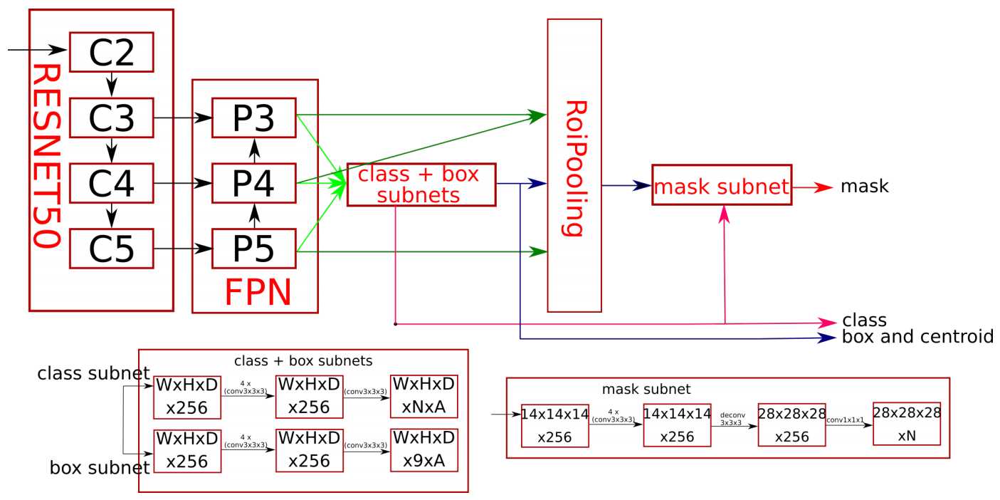
The detector stage. The authors adapt RetinaNet for 3D cases. Their version will also predict the object’s centroid in addition to the axis-aligned bounding box (AABB). The backbone is constructed with a 3D version of the Resnet50 and Feature Pyramid Network (Lin et al. 2018). For this dataset, the authors only use pyramid levels 3 to 5. They avoid level 2 because anchors defined on it are unnecessarily dense for this dataset, while anchors defined on levels greater than 5 are too sparse to distinguish nearby vertebrae. At each pyramid level, they use four anchors with two width/height/depth ratios of 1/1/0.625 and 1/0.74/0.42, and a width of 86 and 68 for level 3, 100 and 79 for level 4 and 120 and 94 for level 5. They are chosen by running a K-means clustering on the AABBs of training vertebrae similar to the algorithm described in (Redmon & Farhadi 2016) to ensure that for each vertebra, they could find at least one anchor so that the Intersection over Union (IoU) with its AABB is higher than 0.6. The classification and regression sub-nets are implemented as described in (Lin et al. 2018). The classification subnet is responsible for the classification of anchors. It predicts a length $N$ one-hot classification vector for each anchor, with $N$ being the number of classes. The regression subnet performs AABB and centroid regression. For each positive anchor, it predicts a length nine regression vector, of which the first 6 encode the AABB (itscentre coordinate and size), and the last 3 encode the centroids’ position. Instead of predicting these values directly, they adopt the coordinate parameterisations of (Ren et al. 2015) for their case.

The mask regression stage. To perform instance segmentation, the authors attach a second stage to their 3D-RetinaNet to output a binary mask for each RoIs detected by the first stage. This stage is implemented similar to Mask R-CNN: a 3D-ROIAlign layer extracts a fixed-size w $\times$ h $\times$ d feature map from the FPN for each RoI using trilinear interpolation, followed by simple fully convolutional networks. These subnets will produce D $\times$ 2w $\times$ 2h $\times$ 2d $\times$ N with D the number of detections provided by the first stage and N the number of classes.

Jakubicek et al.: Approach for Vertebrae Localisation, Identification and Segmentation

The authors propose a fully automatic multi-stage system as shown in Fig. 27. Moreover, they provide an auxiliary semi-automatic mode that enables the inspection and possibly correction of automatically detected positions of the inter-vertebral discs (IVD) and their labels before the following segmentation step. Their approach combines modern deep-learning-based algorithms with more classical image and signal processing steps and with segmentation using the intensity vertebra models adaptation.

Pre-processing. The authors first attempt to cut the data from background and “black" artefacts caused by geometrical shearing. The second step is the correction of the random rotation,which is not presented in the real CT data. For this purpose they provide the CTDeepRot algorithm (Jakubicek et al. 2020), which predicts these rotational angles using a CNN and transforms the data into the standard Head First Supine (HFS) patient position.

Detection of spinal cord centre-line: First, each axial slice of the CT data is classified by a CNN into four categories (slices containing complex C1-2, slices with the main part of the spine from C3 to L6, slices containing the sacrum, and remaining areas feet, head, background). A pre-trained AlexNet (Krizhevsky et al. 2012) CNN is used for this purpose. In the slices containing the main part of the spine, the approximate position of a spinal canal is found (Simonyan & Zisserman 2014) architecture. Each detected centroid of a detected bounding box is taken as a potentially correct centre of the spinal canal in the appropriate axial slice. The whole spinal canal is then traced by the algorithm using the growing inscribed circles, where the detected centroids are taken as starting (seed) points of the tracing. The optimum spine centre-line is then chosen by the population-based optimisation process.

Vertebra localisation and identification. The spine CT data is geometrically transformed into the straightened data according to the spine centre-line curvature. In the straightened data, the centroids of the vertebral bodies are determined by morphological transforms, and the respective intensity profile along the z-axis is taken. This way, the obtained 1D signal is processed by an adaptive IIR (infinite impulse response) filter, which enables detection of the positions of the individual IVDs. Adaptation of the filter is controlled by a statistical model using knowledge about the anatomy of the spine. Finally, each detected IVD is classified into a category of the vertebral type (label) by a combination of a CNN (pre-trained Inception V3 (Guan et al. 2019)) and the dynamic programming optimisation. All used pre-trained CNN architectures were pre-trained on the ImageNet dataset (Russakovsky et al. 2015) and fine-tuned on the authors’ database of CT image data.

Vertebra segmentation. The segmentation of the vertebrae is based on four-step vertebra intensity model registration. In the first step the mean model of the individual vertebra is scaled and deployed along the spine in accordance with the detected and labelled IVDs. The second step performs rigid registration of each vertebra, which aligns the model into an optimally precise position in the 3D CT data, followed by improvement via elastic registration of each vertebra. In the third step, the elastic registration is performed on the whole spine model, where the models fits the shapes of the vertebrae. In the last step, the final segmentation contours are slightly refined and smoothed by the graph-cut based algorithm. Elastix v.5.0.0 (Klein et al. 2009; Shamonin et al. 2014) is sued as the registration software.

Supriti M. et al.: Vertebrae localisation and Segmentation using Mask-RCNN with Complete-IoU Loss

The authors propose to segment vertebrae using Mask-RCNN trained with Complete-IoU (CIoU) loss. The spine vertebrae segmentation process contains the following pipeline: 3D to 2D conversion, pre-processing, Mask-RCNN feature extraction with Complete IoU loss for geometric factor enhancement (Frosio & Kautz 2018), and 2D to 3D back conversion.

3D to 2D conversion. Reorientation of the image is done with flips and reordering the image data array so that the axes match the directions indicated in orientation required for spinal vertebrae segmentation. Reoriented images are resampled to get the balance between image smoothness and identify fine image details.

Preprocessing. CT images reconstructed from low-dose acquisitions may be severely degraded with noise and streak artefacts due to quantum noise, or with view-aliasing artefacts due to insufficient angular sampling. To improve CT image quality median filter along with non-local means (NLM) with Statistical Nearest Neighbors(SNN) by Frosio et al. (Frosio & Kautz 2018) filtering algorithm is applied. Sampling neighbors with the nearest neighbour approach introduces a bias in the denoised patch which improves the CT image quality significantly. Fig. 28(a) and (c) shows the original slice of a spine CT while (b) and (d) shows the enhanced images.

Segmentation using Mask-RCNN with CIoU loss. Mask R-CNN predicts bounding boxes and corresponding object classes for each of the proposed region obtained using a backbone. Following this, a binary mask classifier generates a mask for every class. Bounding box regression is sometimes inaccurate due to overlapping areas. So a complete IoU (CIoU) loss is added in Mask R-CNN.

A good loss for bounding box regression should consider three important geometric factors, i.e. overlap area, central point distance and aspect ratio. Zheng et al. (Zheng et al. 2020) proposed CIoU loss based on these requirements. The authors use an end-to-end pretrained Mask R-CNN-based detectron with CIoU loss model with Resnet x-152 backbone. An existing open-source implementation²² 2 https://github.com/Zzh-tju/DIoU-pytorch-detectron using Pytorch is chosen.

Once the scan is segmented slice-wise in 2D, the final segmentation is obtained by stacking the predicted masks and reorienting and resampling it back to the original image particulars.

Netherton T. et al.: A Multi-view Localisation and Deeply Supervised Segmentation Framework

The authors propose a framework that combines the use of a set of individual CNNs to accomplish 1) course spinal canal segmentation, 2) spine localisation via a multi-view network, and 3) automatic segmentation of individual vertebrae using a deeply supervised approach. A detailed description of steps (1) and (2) of the approach can be found in Netherton et al. 2020. Refer to Fig. 29 for an overview of the proposed approach.

Data. Data from VerSe 2019 and 2020 was used to train localisation and segmentation CNNs. All images and segmentations were resampled to have isotropic voxel sizes (1.0mm³) and set to a common orientation. Ground truth localisation coordinates were not used in this approach. In total, 160 pairs of CT scans and segmentations were obtained and split into five groups for cross-validation.

Spinal canal segmentation. First, the spinal canal is segmented via a 2-dimensional FCN-8s with batch normalisation on the axial CT slices. Pairs of intensity projection images (sagittal and coronal) are then generated about a volume of interest (cropped from the CT scan) surrounding the spinal canal. These image pairs provide the network with sagittal and coronal views of the vertebral column and have a fixed width but variable length $l$ (where $l$ is the length of the CT scan); their corresponding ground-truth labels are then assigned individual channels (27 total) to account for each vertebral level. For the training stage, planar segmentation masks posterior to the spinal canal are removed to produce modified vertebral coordinates. In order to provide a large number of image augmentations, intensity projection image pairs (and corresponding ground truth masks) are incrementally cropped from the superior-inferior, inferior-superior, and medial-lateral directions.

Multi-view spinal localisation. X-Net (Netherton et al. 2020), the localisation architecture, inputs the sagittal and coronal intensity projection pairs and outputs labeled, multi-dimensional sagittal and coronal arrays of individual vertebral column segmentations. X-Net, inspired by Sekuboyina et al. 2020 and Milletari et al. 2016, incorporates residual connections, pReLU activations, and is end-to-end trainable. By combining centre-of-mass coordinates from sagittal and coronal planar segmentations, 3-dimensional locations are obtained for each vertebral body. During training, the loss function, which incorporated the soft-Dice loss and cross-entropy loss, was applied to each view (i.e. coronal and sagittal, $L=L_{s}+L_{c}$ ). Augmentations were applied during training with a frequency of 0.7; coronal arrays were flipped left-right with a frequency of 0.5. Training was performed on a 16GB NVIDIA-V100 with batch size 8. Each model was trained for at least 26,000 iterations using early stopping.

Deeply supervised vertebral body segmentation. To perform vertebral body segmentation, a UNet++ architecture using skip connections, multi-class structure, and deep supervision is designed based on work by (Zhou et al. 2019) . Using ground truth images and segmentations, three channel arrays are formed for each vertebral level by cropping around the centre of mass of each vertebral level. Separate channels contained background, adjacent vertebral levels, and the central vertebral level, respectively. For each 3-dimensional coordinate (from the second stage), the CT scan is cropped to form separate volumes of interest (120 $\times$ 96 $\times$ 96mm³). The top two most supervised outputs from each prediction are averaged to yield the vertebral body of interest.

Paetzold J. et al.: A 2D-UNet on the VerSe data

The authors implement a 2-D segmentation architecture for slices of the sagittal orientation of the 3-D dataset using a 2D U-Net (Ronneberger et al. 2015). The encoder is made of a ResNet-34 backbone pre-trained on the ImageNet. The network is trained by optimising an equally weighted sum of the Dice loss and the binary cross-entropy loss (BCE) with data augmentations such as flipping, rotation, scaling, and shifting. The images are centre-cropped to 512 by 512 pixels to account for the irregular image sizes during training. All networks are implemented in Pytorch using the Adam optimiser and are trained for 1000 epochs. After prediction, the 2D slices are stacked together to reconstruct the 3D volume. The training was carried out on an NVIDIA QUADRO RTX 8000 GPU with a batch size of 52.

Xiangshang Z. et al.: Vertebra Labelling and Segmentation using the Btrfly-net and the nnU-net

The authors design an improved Btrfly Network (Sekuboyina et al. 2018) to detect the key points of the vertebrae and then build an nn-Unet (Isensee et al. 2019) to segment the vertebral regions. Both the labelling and segmentation tasks are handled independently.

Vertebra Labelling. Similar to Sekuboyina et al. 2018, the authors work with 2D sagittal and coronal MIP. Improving on it, changes were made to the model architecture and the training procedure. Two convolution layers for each layer of encoder and decoder in the network followed by batch-normalisation and ReLU non-linearity after each convolution layer. Kaiming-initialisation is used for the network parameters. In terms of data-based enhancements, the authors use horizontal and vertical flip for augmentation and with normalisation.

Vertebra segmentation. The preprocessing and training procedure of the nnU-Net is retained. On top of it, data augmentation is applied on the fly during training using the batch-generators framework (Isensee et al. 2020). Specifically, elastic deformations, random scaling, and random rotations are used. If the data is anisotropic, the spatial transformations are applied in-plane as 2D transformations. Once trained, cases are predicted using a sliding window approach with half the patch size overlap between predictions.

Yeah T. et al.: A Coarse-to-Fine Two-stage Framework for Vertebra Labeling and Segmentation.

The author propose a two-stage network to achieve vertebra labeling and segmentation. Firstly, the low-resolution net determines the rough target location from downsampled CT images. Secondly, by feeding the first stage’s prediction results (upsampling before feeding) and high-resolution CT scans into a full resolution net, more accurate vertebra classification and segmentation are achieved. Considering the competition among different vertebra classes especially for adjacent vertebra, finally connected component analysis is applied to refine vertebrae segmentation results.

The two-stage cascaded segmentation pipeline consists of two steps. Firstly a coarse location of spine RoI is obtained based on a lightweight low-resolution 3D U-Net from 3D CT scans with low resolution. Secondly the RoI and the accurate segmentation results are performed with a high-resolution 3D U-Net. Finally some post-processing methods are adopted to fill the holes inside each vertebrae and rule-based methods to recalibrate the vertebrae label. Both the low-resolution network and the high-resolution network have 26 output channels (C1-C7, T1-T13, L1-L6).

The first stage preprocesses the training 3D CT scans to a larger spacing through downsampling and train the low-resolution 3D U-Net model with a patch size of 224 $\times$ 128 $\times$ 96. The second stage preprocesses 3D CT images to smaller spacing through upsampling and crops the RoI of spine regions as the training dataset for a high-resolution U-Net model with a patch size of 256 $\times$ 96 $\times$ 80.

Preprocessing and Augmentation. All input images are normalised zero mean and unit standard deviation (based on foreground voxels only). The data augmentation include elastic deformation, rotation transformation, gamma transformation, random cropping, etc.

Loss and Optimisation. The low-resolution model with a classical combination of Dice loss and cross-entropy loss, while training the high-resolution model with a dynamic hybrid loss combining Dice loss and weighted cross-entropy loss. A model with a dynamic hybrid loss combining Dice loss and Adam optimiser with an initial learning rate of 10^-4 was used. During training, an exponential moving average of the validation and training losses is used. Whenever the training loss does not improve within the last 30 epochs, the learning rate is reduced by factor 5. The training is terminated automatically if validation loss does not improve within the last 50 epochs.

Zeng C.: Two-stage Keypoint Location Pipeline for Vertebrae Location and Segmentation.

The author proposes a two-stage keypoint detection pipeline for vertebral labeling based on the scheme of Payer et al. 2019 which uses Spatial-Configuration-Net and U-Net in VerSe‘19 described in Section 3.

Additional Data and Preprocessing. An additional 13 data sets from the VerSe‘19 training set are used. The data is first preprocessed to the RAI direction. Data augmentation includes rotation, intensity shift, scaling and elastic deformation. The model is trained with all 113 cases.

Localisation. To localize centres of the vertebrae, five keypoints location and global vertebrae location is performed separately. For the five keypoints, which contains the first and last two vertebral masses of the cervical spine, thoracic spine and lumbar spine, a network is designed of which the backbone is an HRNet (Sun et al. 2019) to regress the five keypoint heatmaps. The significance of the first stage is for better identification of several vertebral masses with obvious characteristics. The second stage follows Payer et al. 2019, with a re-designed channel attention block in the network with a weighted loss function.

Vertebrae Segmentation. For vertebrae segmentation, a binary segmentation network is trained based on the outcome of the labelling stage. A U-Net with an inputs size of 128 $\times$ 128 $\times$ 64 is used. The loss function is a mixture of Dice loss and binary cross-entropy loss.

Zhang A. et al.: A Segmentation-Based Framework for Vertebrae Localisation and Segmentation.

In general, the vertebrae localisation and segmentation tasks are performed in a four-step approach: 1) spine localisation to obtain the region of interest, 2) single-class key point localisation to obtain the potential vertebrae candidates, 3) a triple-class vertebrae segmentation to obtain the individual mask and main category of each vertebrae, and 4) rule-based post-processing.

A variant of V-Net with a mixture of Dice and binary cross-entropy loss is utilised in the first three steps and only a few hyperparameters are changed in each step, such as input/output shape, depth, width, etc. Step 2 and step 3 could be corrected by each other in an ‘intertwined’ way as mentioned above: the proposed key-point candidates are used as input for step 3 to specify the vertebra to be segmented if the resulting segmentation result does not seem to be a mask (the volume is not large enough), then the proposed key-point can be regarded as a false positive.

Spine Localisation. To obtain the spinal centerline, a variant of V-Net is used to regress a heatmap of the spinal centerline. The input is a 4-time downsampled single-channel 3D-patch with a size of 64 $\times$ 64 $\times$ 64). The sliding window approach is applied to serve the network with the specific size of local cubes. The heatmaps are generated using a Gaussian kernel by a kernel size (5, 5, 5) and sigma (6, 6, 6) on the downsampled mask to keep unique 3D connected domain. The output heatmap is converted to a binary mask by a threshold of 0.4 and resampled back to the origin image scale for later use.

Keypoint Localization. A similar variant of V-Net is employed to regress a heatmap of the spine. The input in this step is a single-channel 3d-patch with the size of 64 $\times$ 128 $\times$ 128. Sliding window approach is applied as above. The heatmaps are generated by kernel size (7, 9, 9) and sigma (6, 6, 6) on the original scale based on the JSON label to ensure they are independent and disconnected. The proposed regression results are converted to a binary mask by a threshold of 0.4 and the centroid is calculated for each cluster.

Vertebrae Segmentation. Considering half of the vertebrae account for a lack of samples for a 26-class classification, a triple-class segmentation task is defined to segment three categorises: ‘cspine’, ‘tspine’ or ‘lspine’ for each vertebra in this step. A variant of V-Net is employed. The input is a cropped 3D patch around the localised centroid obtained from step 2.

Rule-based Post-processing. In this step a simple post-preprocessing logic is applied to create the final multi-label result. If more than one category of vertebrae is found in one case, the two or four ‘split points’ which is C7-T1 and T12-L1 can be localised. Then the others can be deduced based on these split points. If split points are not found in one case, then ‘cspine’ vertebrae are deduced from C1 to the bottom and ‘lspine’ ones are deduced from the bottom to the top.

VerSe: A Vertebrae Labelling and Segmentation Benchmark for Multi-detector CT Images