Magnetohydrodynamic Simulations of Binary Neutron Star Mergers in General Relativity:
Effects of Magnetic Field Orientation on Jet Launching
Abstract
Binary neutron star mergers can be sources of gravitational waves coincident with electromagnetic counterpart emission across the spectrum. To solidify their role as multimessenger sources, we present fully 3D, general relativistic, magnetohydrodynamic simulations of highly spinning binary neutrons stars initially on quasicircular orbits that merge and undergo delayed collapse to a black hole. The binaries consist of two identical stars modeled as polytropes with spin aligned along the direction of the total orbital angular momentum . Each star is initially threaded by a dynamical unimportant interior dipole magnetic field. The field is extended into the exterior where a nearly force-free magnetosphere resembles that of a pulsar. The magnetic dipole moment is either aligned or perpendicular to and has the same initial magnitude for each orientation. For comparison, we also impose symmetry across the orbital plane in one case where in both stars is aligned along . We find that the lifetime of the transient hypermassive neutron star remnant, the jet launching time, and the ejecta (which can give rise to a detectable kilonova) are very sensitive to the magnetic field orientation. By contrast, the physical properties of the black hole + disk remnant, such as the mass and spin of the black hole, the accretion rate, and the electromagnetic (Poynting) luminosity, are roughly independent of the initial magnetic field orientation. In addition, we find imposing symmetry across the orbital plane does not play a significant role in the final outcome of the mergers. Our results suggest that, as in the black hole-neutron star merger scenario, an incipient jet emerges only when the seed magnetic field has a sufficiently large-scale poloidal component aligned to the initial orbital angular momentum. The lifetime [] and Poynting luminosities [erg/s] of the jet, when it forms, are consistent with typical short gamma ray bursts, as well as with the Blandford–Znajek mechanism for launching jets.
pacs
04.25.D-, 04.25.dk, 04.30.-w, 47.75.+fI Introduction
The exciting prospect of simultaneous observations of both gravitational waves (GWs) and electromagnetic (EM) signals originating from the coalescence and merger of binary neutron stars (NSNS) makes these systems, along with black hole-neutron star (BHNS) binaries, prime targets for the LIGO/Virgo scientific collaboration in the era of multimessenger astronomy (MA). These systems had long been hypothesized as progenitors of the same central engines that power short-hard gamma-ray bursts (sGRBs), see e.g. Paczynski 1986; Eichler et al. 1989; Narayan et al. 1992, which was strongly supported by the first detection of a kilonova associated with the sGRB “GRB130603B” Tanvir et al. 2013; Berger et al. 2013.
The strongest theoretical support for this hypothesis came from self-consistent, fully general relativistic magnetohydrodynamic (GRMHD) simulations of BHNS and NSNS mergers Paschalidis et al. 2015a; Ruiz et al. 2018a; Ruiz et al. 2016; Ruiz and Shapiro 2017 that showed that an incipient jet may be launched if the NS is suitably magnetized. Nevertheless, the detection of GW170817 Abbott et al. 2017a coincident with a sGRB (event GRB170817A Abbott et al. 2017b), as well as its association with kilonova AT 2017gfo/DLT17ck Valenti et al. 2017, provides the best direct observational evidence so far that some sGRBs are indeed powered by NSNS mergers, or at least by the merger of a compact binary where at least one of the companions is a NS. Note that the progenitor of GW170817 has been identified as an NSNS based on the masses of the companions; depending on the spin priors of the binary companions, their inferred masses are in the broad range of , though the total mass of the system is constrained to be with credibility Abbott et al. 2017a. These masses are consistent with astrophysical observations of NSs (see e.g. Özel and Freire 2016; Lattimer and Prakash 2016; Bogdanov et al. 2019a; Bogdanov et al. 2019b), but it cannot rule out the presence of a stellar-mass BH Foucart et al. 2018. Recently, X-ray observations have strongly suggested that the rapidly rotating, giant star 2MASS J05215658+4359220 is the binary companion of a noninteracting BH Thompson et al. 2019. So, there may be a population of stellar-mass BHs missed by X-ray observations that eventually may form GW170817-like binary systems. Mechanisms and routes by which stellar-mass BH formation may arise in binaries with NS companions were recently discussed in Yang et al. 2018.
The GRMHD simulations of BHNSs mergers reported in Paschalidis et al. 2015a; Ruiz et al. 2018a, in which the NSs are modeled as irrotational polytropes, have shown that these systems, evolved from the late inspiral through tidal disruption, merger, and settling, can launch a magnetically-supported incipient jet. The lifetime of the jet [s] and its outgoing Poynting luminosity [ ] turn out to be consistent with typical sGRBs Bhat et al. 2016; Lien et al. 2016; Svinkin et al. 2016; Ajello et al. 2019, as well as with the Blandford-Znajek (BZ) mechanism for launching jets and their associated Poynting luminosities Blandford and Znajek 1977a. Here is the rest-mass of the NS. The key requirement for jet launching is the existence of a large-scale poloidal magnetic field component with a consistent sign in the vertical direction threading the BH + disk remnant Beckwith et al. 2008; Beckwith et al. 2009. These magnetic components can be obtained by endowing the NS with a dipolar magnetic field resembling that of pulsars, with the dipole moment along the direction of the total angular momentum of the system. The presence of the dipole field ensures that the BH poles will be threaded with poloidal magnetic lines before tidal disruption, whereby a significant poloidal component of the field will remain after the disruption. Differential rotation in the accretion disk winds up the field lines, converting poloidal flux into toroidal flux. The magnetic field then is amplified to G above the BH poles and wound into a helical funnel, inside which fluid elements from the accretion disk flow outward with Lorentz factors at launch of . We say that, at this point, an incipient jet has emerged. By contrast, if the initial magnetic field is confined to the NS interior, the frozen-in magnetic field following the NS disruption is wound into a nearly toroidal configuration (see e.g. Etienne et al. 2012), and hence jet formation is suppressed.
The GRMHD simulations of NSNS mergers, in which the NS is modeled as polytrope, show that an incipient jet can be launched whether or not the seed poloidal magnetic field is confined to the interior of the NS as long as the binary forms a transient hypermassive remnant before undergoing delayed collapse to a BH Ruiz et al. 2016; Ruiz and Shapiro 2017; Ruiz et al. 2019. In this case, in contrast to the prompt collapse case (see e.g. Totani 2013; Paschalidis and Ruiz 2019 for possible EM counterparts in this case), the formation of a hypermassive neutron star (HMNS) allows magnetic instabilities to amplify the magnetic energy to reach equipartition with the plasma kinetic energy before BH formation Kiuchi et al. 2014. Following the HMNS collapse, a magnetically–supported jet is then launched once the regions above the BH poles approach force-free values (). Here and are the strength of the magnetic field and the rest-mass density, respectively. As in the BHNS case, the lifetime of the jet and its associated Poynting luminosity are consistent with typical sGRBs Bhat et al. 2016; Lien et al. 2016; Svinkin et al. 2016; Ajello et al. 2019, as well as with the BZ mechanism. Note that in the GRMHD simulations reported in Kawamura et al. 2016; Ciolfi et al. 2017; Kiuchi et al. 2014, where the magnetic field is confined to the NS interior, neither an outgoing outflow nor a jet were observed. The lack of a jet in Kawamura et al. 2016; Ciolfi et al. 2017, where the effects of realistic equations of state (EOSs), mass ratios, and orientations of the seed poloidal magnetic field were probed, is likely due to the incomplete development of the magneto-rotational-instability (MRI), which is required to boost the magnetic field strength, though the formation of an organized helical structure above the BH was evident (see e.g. Fig. 9 in Kawamura et al. 2016). The absence of a jet in the very high-resolution studies in Kiuchi et al. 2014, in which an H4 EOS is used to model the NS, can be attributed to the persistent fall-back environment that increases the downward ram pressure above the BH poles. These studies may require longer simulations ( ms after merger) for a jet to emerge as long as the matter fall-back timescale is shorter than the accretion disk lifetime Paschalidis 2017. In all the above numerical studies reflection symmetry across the orbital plane was imposed.
As the key requirement for jet launching in the NSNS scenario seems to be the amplification of the magnetic field during the HMNS epoch, one might tentatively conclude that NSNS mergers undergoing delayed collapse to a BH can lead to jets under a wide variety of initial magnetic field configurations. But, is this enough? It has been suggested that pure poloidal magnetic field configurations may be unstable over an Alfvén timescale (see e.g. Markey and Tayler 1973; Wright 1973). Full 3D Newtonian simulations, and recent full 3D general relativity simulations using the Cowling approximation, showed that nonrotating and isolated stars endowed with pure poloidal components may relax into a new configuration with both poloidal and toroidal magnetic components of similar strengths (see e.g. Braithwaite and Spruit 2004; Ciolfi and Rezzolla 2012; Ciolfi et al. 2011). But, is this new magnetic field configuration suitable for jet launching? Moreover, if GW radiation and magnetic turbulent viscosity drive the bulk of the HMNS into a purely axisymmetric configuration, the sustained amplification of the magnetic field is, according to the anti-dynamo theory Moffatt 1978, no longer possible. If so, is the BH + disk remnant an EM counterpart orphan?
To address the above questions, we perform full 3D GRMHD simulations of NSNS configurations in quasicircular orbits that merge and undergo delayed collapse to a BH. The binaries consist of two identical, uniformly rotating NSs modeled with a polytropic EOS with spin , where is the quasilocal angular momentum of the NS, and is the Arnowitt-Deser-Misner (ADM) mass of the system Tsokaros et al. 2018. We choose highly spinning NSNS configurations to reduce computational costs, because, as we recently showed in Ruiz et al. 2019, the higher the initial spin of the binary companions the shorter the jet launching time. We adopt a polytropic EOS for a direct comparison with our previous results (see e.g. Ruiz et al. 2016; Ruiz and Shapiro 2017; Ruiz et al. 2019). Each star is initially endowed with a dipolar magnetic field of the same magnitude extending from the stellar interior into its exterior and whose dipole moment is either aligned or perpendicular to the direction of the total orbital angular momentum of the system . We consider the following configurations:
- 1.
Ali-Ali case: The magnetic dipole moment in both stars is aligned to .
- 2.
Ali-Per case: The magnetic dipole moment in one of the stars is aligned to , while in the other is perpendicular to it.
- 3.
Per-Per case: The magnetic dipole moment in both stars is perpendicular to .
Note that these three cases can be used to infer the outcome of general cases in which the dipole moment of the seed magnetic field is misaligned by an angle to the spin of the NS. For comparison purposes, we also consider a second Ali-Ali case in which symmetry across the orbital plane (equatorial symmetry) is imposed. This case has been treated previously in Ruiz et al. 2019, and it will be denoted here as Ali-Ali (Eq).
As in Ruiz et al. 2019, in all our cases we find that, following the NSNS merger, magnetic braking due to turbulent magnetic fields in the bulk of the transient HMNS induces the formation of a uniformly rotating central core immersed in a low-density Keplerian cloud of matter. Depending on the initial orientation of the magnetic dipole moment, the HMNS collapses to a BH in a timescale of following the NSNS merger, the shortest one being for the Ali-Ali and Ali-Ali (Eq) cases and the longest one for the Per-Per case. The mass and spin of the BH, as well as the rest-mass of the accretion disk, are roughly independent of the initial magnetic field configuration. However, we find that, as in the BHNS cases reported in Ruiz et al. 2018a, an incipient jet is launched only when the system has initially a large-scale poloidal magnetic field component aligned to the initial angular orbital momentum. The lifetime of the incipient jet [] and its outgoing Poynting luminosities [], when it forms, are consistent with typical sGRBs Bhat et al. 2016; Lien et al. 2016; Svinkin et al. 2016; Ajello et al. 2019, as well as with the BZ mechanism for launching jets Blandford and Znajek 1977b. We also observe that only in Ali-Ali cases does a significant fraction of the rest-mass () become unbound and hence may lead to a kilonova signal observable by current telescopes, such as the Large Synoptic Survey Telescope (LSST) Shibata et al. 2017; Rosswog 2005. Although our preliminary GRMHD simulations do not account for all the physical processes involved in NSNS mergers, they indicate that, as the ejecta is highly affected by the configuration of the magnetic field prior to the merger, NSNS merger models without magnetic fields that are used to explain the early part of the radioactive powered kilonova signal (blue luminosity) linked to GW170817 may overestimate the amount of escaping matter.
We also probe whether different seed magnetic field orientations could be distinguishable by current GW detectors. Assuming a source distance of Mpc, we compute the match function and find that the GWs of Ali-Ali and Per-Per are distinguishable for a signal-to-noise ratio , while in the other cases, they can be distinguished with a signal-to-noise ratio . As GW150914 (first GW detection of BHBH) and GW170817 (first GW detection of NSNS) events were observed with a signal-to-noise ratio of and Abbott and et al. 2016; Abbott et al. 2017a, respectively, current GW detectors may, in principle, be able to distinguish effects induced by different magnetic field configurations.
The paper is organized as follows. A short summary of the numerical methods and their implementation, initial data, grid setup, and global diagnostic checks are given in Sec. II. For further details, readers are referred to Ruiz et al. 2019. Sec. III.1 contains a detailed comparison of the evolution of Ali-Ali in both equatorial symmetry and full 3D. Secs. III.2 and III.3 describe the evolution of the Ali-Per and Per-Per cases, along with a comparison with the previous cases. In Sec. III.4 we assess the distinguishability of the GWs for the different cases. We summarize our findings and conclude in Sec.IV. Throughout the paper, we adopt geometrized units () except where stated otherwise. Greek indices denote all four spacetime dimensions, while Latin indices imply spatial parts only.
II Numerical Setup
The following section summarizes the key aspect of our numerical approach.
Numerical Methods:
We use the GRMHD code developed by the Illinois Numerical Relativity Group Etienne et al. 2010, which is embedded in the Cactus infrastructure Cactus and uses Carpet Carpet for moving boxes refinement. It employs the BSSN evolution equations Shibata and Nakamura 1995; Baumgarte and Shapiro 1999, with fourth-order centered spatial differencing, except on shift advection terms, where a fourth-order upwind differencing is used, coupled to the puncture gauge conditions (see Eq. (2)-(4) in Etienne et al. 2008). In all our evolution, we set the damping coefficient appearing in the shift condition to , with the ADM mass of the system. Time integration is performed using the Method of Lines with a fourth-order Runge-Kutta integration scheme and a Courant-Friedrichs-Lewy factor equal to . For numerical stability, we add fifth-order Kreiss-Oliger dissipation Baker et al. 2006 in the BSSN evolution equations. Also, a dissipation term in the evolution equation for the conformal factor is added to damp the Hamiltonian constraint violations (see Eq. 19 in Duez et al. 2003).
Initial Data:
We use the Compact Object CALculator (COCAL) code to generate the initial NSNS configurations on a quasicircular orbit (see e.g. Tsokaros et al. 2015; Tsokaros et al. 2016; Tsokaros et al. 2018 for numerical details). Specifically, we use the , spinning NSNS configuration listed in Table 1 of Ruiz et al. 2019, for which the ADM mass of the system is , and has an initial coordinate separation of . Each binary companion has a quasilocal dimensionless spin parameter [or a rotational period ] aligned with orbital angular momentum of the system Tsokaros et al. 2018, a rest mass of and compactness . Here is the polytropic constant used to generate the initial data where . Note that for an polytrope, the maximum mass configuration has , and .
We initially endow the star with a dipole-like magnetic field whose dipole moment is either aligned or perpendicular to the the total angular momentum of the system . Following Ruiz et al. 2019, the seed magnetic field in the aligned case is generated by the vector potential (see top panels in Fig. 1)
| (1) |
induced by a current loop inside the star with radius , where , , and is the center of mass of the NS, defined here as the position of the maximum value of the rest-mass density of each NS. We choose and such that the maximum value of the magnetic-to-gas pressure ratio is at the center of each star. With this choice, the resulting magnetic field strength at the NS pole is initially . As pointed out in Ruiz et al. 2016, this magnetic field strength is used to mimic the result of exponential growth of the magnetic field due to the Kelvin-Helmholtz instability (KHI), along with the MRI, triggered during the NSNS merger and HMNS formation. However, this growth is captured only in very high-resolution [] NSNS simulations (Kiuchi et al. 2014; Kiuchi et al. 2015); during merger the rms value of the magnetic field strength is boosted from to , with local values up to .
Equatorial symmetry Full 3D


In the perpendicular case, on the other hand, we keep the same magnetic-to-gas-pressure ratio at the center of mass of the NS but rotate counterclockwise the Cartesian components of the above vector potential by (see top panel in Fig. 2 and top left panel in Fig. 3).
Following Ruiz et al. 2018a, to mimic the “force-free” magnetosphere surrounded the NS, and to reliably evolve the magnetic field outside the star, we set a variable exterior, low-density magnetosphere such as that is everywhere. This density increases the total rest-mass of the system by Ruiz et al. 2016. For the subsequent evolution, as is typically done in standard hydrodynamics schemes, we integrate the ideal GRMHD equations everywhere, imposing on top of the magnetosphere a density floor in regions where . Here is the initial maximum rest-mass density of the system.
Grid structure:
In all simulations, we use seven refinement levels with two sets of nested refinement boxes (one for each NS and centered in its center of mass), differing in size and resolution by factors of two. The innermost refinement level around each star has a side length of , where is the initial NS equatorial radius, and a grid spacing of . With this choice the initial NS equatorial radius is resolved by grid points, which matches the resolution used in Ruiz et al. 2019. We also rerun the Per-Per case at a resolution of . Finally, the outer boundary is located at .
Diagnostics:


To analyze and check the reliability of the evolution of our binary systems, we use the following tools:
- •
Global diagnostic checks: To validate the numerical integration, we monitor the norm of the normalized Hamiltonian and momentum constraints computed using Eqs. (40)-(41) in Etienne et al. 2008. In all our cases (see Table 1) we find that during the inspiral and HMNS evolution phase, the constraints remain below . They peak at during BH formation and settle back to after the BH + disk remnant reaches quasi-equilibrium. We also monitor the conservation of both the ADM mass and the ADM angular computed using Eqs. (19)-(22) in Etienne et al. 2012. By the end of the simulations we find that, in all configurations, the violation of the conservation is , while the violation of the conservation of is . Similar values were reported in our long-term, pure hydrodynamic simulations of spinning NSNS modeled by piecewise EOSs Tsokaros et al. 2019. The above calculations take into account the GW radiation losses and the ejected material following merger; to measure the energy and angular momentum carried off by GWs, we use a modified version of the Psikadelia thorn that computes Ruiz et al. 2008 at different radii between and . Around of the total energy, and of the angular momentum, is radiated away (see Table 1). The escaping mass, i.e. unbound fluid elements satisfying with positive radial velocity, is computed as outside a coordinate radius . Here is the lapse, is the determinant of the 3-metric, is the time-component of the 4-velocity, and is the rest-mass density. Depending on the initial configuration of the magnetic field, between and of the total rest-mass of the system is ejected.


Figure 3: Volume rendering of rest-mass density , normalized to the initial maximum value (log scale), at selected times for the Per-Per case. White lines represent the magnetic field lines. Bottom panels highlight the final configuration of the BH + disk remnant. - •
Post-merger diagnostics: To probe if magnetic instabilities are triggered during the formation and evolution of the transient HMNS, we monitor the growth of the magnetic energy measured by a comoving observer. Once the HMNS has settled down, we compute the quality factor that measures the number of grid points per fastest-growing MRI mode. Here is the fastest-growing MRI wavelength. A is required to properly capture the MRI Shiokawa et al. 2012; Sano et al. 2004. MHD turbulence is also diagnosed via the effective Shakura–Sunyaev parameter , where is the component of the EM stress energy tensor computed using the orthornormal contravariant tetrad system in the local fluid-frame Penna et al. 2010. Following Gold et al. 2014, we report an azimuthally- and - averaged profile. Finally, to measure the degree of differential rotation of the HMNS, we monitor its azimuthally-averaged angular velocity using Eq. 2 in Ruiz et al. 2019.
- •
Post-collapse diagnostics: We adopt the AHFinderDirect thorn Thornburg 2004 to locate and monitor the apparent horizon (AH), and the isolated horizon formalism Dreyer et al. 2003 to measure the mass of the BH and its dimensionless spin parameter . Following BH formation, the outgoing EM Poynting luminosity is computed via across different spherical surfaces of coordinate radii between and . To assess whether the magnetic field above the BH remnant poles is sufficiently strong to launch a jet we compute the force-free parameter , where , with the magnetic field measured by an observer co-moving with the fluid. When it exceeds a jet is typically launched via the BZ mechanism Paschalidis et al. 2015a. Finally, we compute the rest-mass accretion rate via Eq. A11 in Farris et al. 2010.
III Results
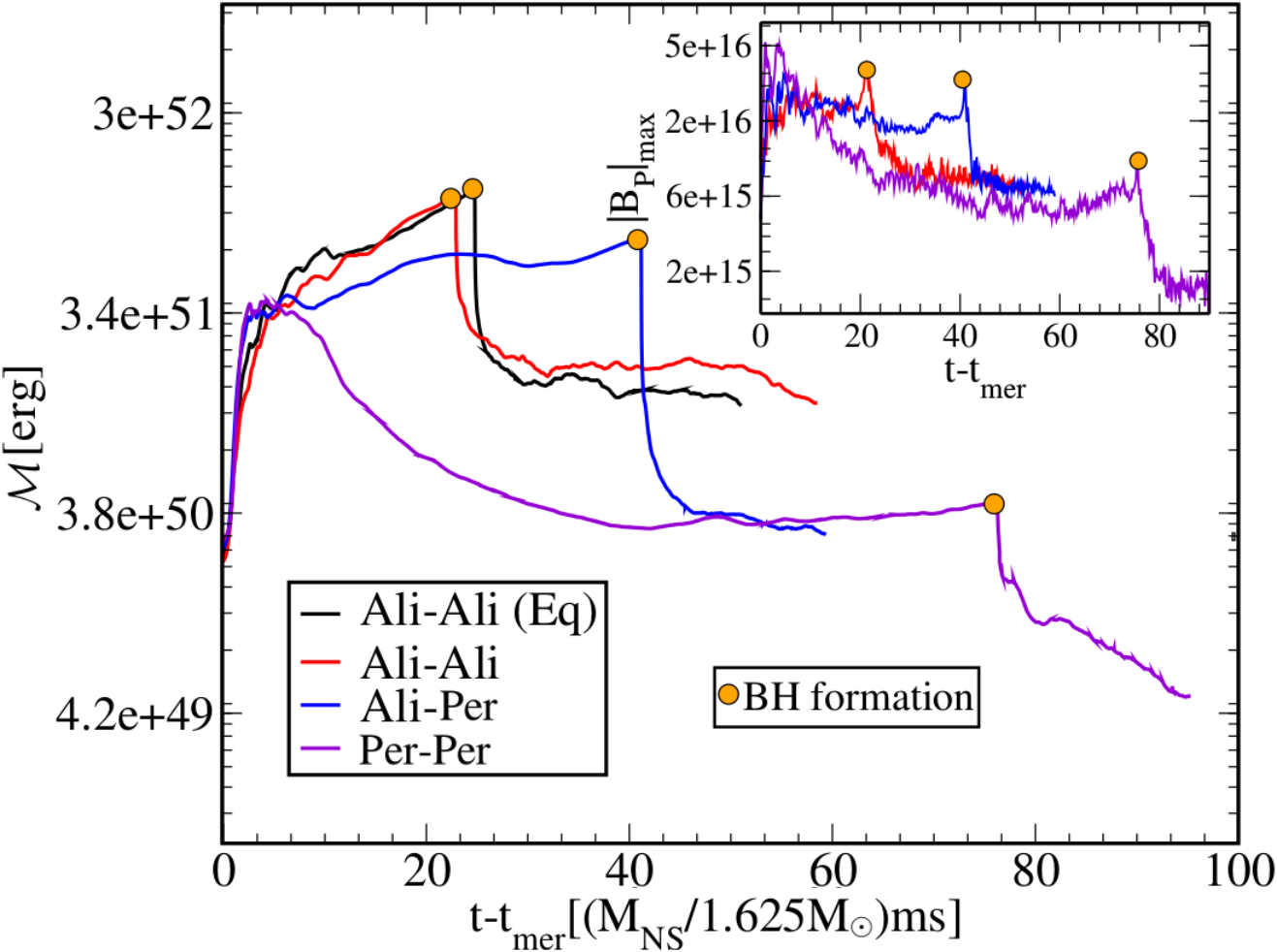
The basic dynamics of our NSNS configuration has been described in Ruiz et al. 2019. As the GWs carry off energy and angular momentum, the orbital separation decreases. After roughly orbits (or GW cycles, see inset in Fig. 4) the stars merge, forming a transient remnant with two massive central cores rotating about each other. After , these cores collide and give birth to a magnetized and highly differentially rotating HMNS surrounded by a Keplearian-like cloud of low density matter. As shown in the inset of Fig. 5, during the HMNS formation the strength of the poloidal magnetic field component peaks at , consistent with the values reported in the high-resolution studies in Kiuchi et al. 2015. As pointed out in Ruiz et al. 2016, the toroidal magnetic field component is also amplified until it approximately equals the magnitude of the poloidal one.
Effective turbulence induced by magnetic fields leads to the transport of angular momentum from the rapidly rotating inner layers of the HMNS to the slowly rotating outer part (see Fig. 6). It causes the central part of the HMNS to contract, forming a nearly uniformly rotating, massive central core that contains roughly of the total rest-mass of the system. As rigid rotation does not provide enough centrifugal support to the central core to prevent collapse (i.e. its mass exceeds , the maximum mass allowed by a uniformly rotating star Cook et al. 1994; Lyford et al. 2003), it eventually collapses, forming a highly spinning BH surrounded by a Keplerian accretion disk. As we show in the following section, only if the NSNS has initially a large-scale strong poloidal component aligned to the orbital angular momentum of the system, does the BH + disk remnant eventually launch a large-scale, magnetically-sustained outflow. The summary of the key results is presented in Table 1.

III.1 Both aligned magnetic fields: equatorial symmetry vs. full 3D evolutions
Fig. 1 shows a side-by-side comparison of the evolution of the Ali-Ali configuration in both equatorial symmetry (left column) and full 3D (right column) at selected times. Colors depict the rest-mass density , normalized to its initial maximum value , white lines shows the magnetic field lines, while arrows indicate plasma velocities.
As shown in the top panel of Fig. 4, symmetries do not have a significant effect on the dynamics of stars during the inspiral. During this epoch, the binary companions orbit each other, dragging the frozen-in magnetic field with them. Gravitational radiation extracts energy and angular momentum and drives the system to an unstable orbit. The stars come into contact with another for the first time at (see Table 1). We observer that the configuration in full 3D merges around earlier than in the equatorial case. Here, the merger time is defined as the time of the peak amplitude of GWs (see Fig. 4). As shown in the second row of Fig. 1, during merger the stars become oblate with spiral arms that wrap around the nascent remnant, forming a cloud of low-density matter. The central regions of the stars begin to orbit around each other, and eventually, collide to form a magnetized HMNS. Due to the KHI, along with the MRI, the magnetic energy is steeply enhanced Kiuchi et al. 2014; Kiuchi et al. 2015. Fig. 5 shows that during the first , is amplified by a factor of . Afterwards, and roughly during the next up to the BH formation, grows by a factor of . We notice that the magnetic field amplification saturates once the poloidal and the toroidal components reach a magnitude of (see inset of Fig. 5).
Once the HMNS has settled down, we probe whether magnetic instabilities have been triggered. We first compute the quality factor and find that of the fastest-growing MRI is resolved by grid points and it fits within the star. We conclude that MRI is resolved and operating in our system, as expected from our previous simulations in Ruiz et al. 2019 (see Fig. 9 in there). Moreover, we find that for , the effective Shakura–Sunyaev viscosity parameter is (see Table 1). Here brackets denote an average over one stellar rotation period (see Fig. 6). Similar values were reported in high-resolution simulations of strongly massive NS remnants in Kiuchi et al. 2018. Thus, magnetic turbulence is likely to be fully developed in the transient HMNS Kiuchi et al. 2018. However, magnetic turbulence can be suppressed by numerical diffusion Kiuchi et al. 2018; Hawley et al. 2011; Hawley et al. 2013 and, therefore, the value of in our simulations may be underestimated. As pointed out in Kiuchi et al. 2018, higher resolutions are required to properly model magnetic turbulence (see also Hawley et al. 2011; Hawley et al. 2013 for a detailed discussion).
Differential rotation and turbulent magnetic viscosity triggers magnetic braking Sun et al. 2019 which causes the formation of a massive and highly oblate central core. The core is immersed in a cloud of matter originating from the expansion of the external layers of the HMNS (see the third row of Fig. 1). The flow in the central core drives the poloidal field lines to a toroidal configuration (magnetic winding). The toroidal magnetic field is then amplified until its magnitude equals the strength of the poloidal component. We notice that by , the shape of the HMNSs in the two Ali-Ali cases (equatorial symmetry and full 3D case) is basically the same, though the magnetic field, in the full 3D evolution, has been wound into a larger-scale helical structure (see the third row of Fig. 1).


By (see Table 1), the central core has approached rigid rotation (see left panel in Fig. 6), and collapses to a BH. Note that this timescale is consistent with magnetic braking induced by magnetic winding (the Alfvén timescale), which can be estimated as (see Eq. 2 in Sun et al. 2019):
| (2) | |||||
where is the characteristic radius of the HMNS remnant and the Alfvén speed, with the strength of the magnetic field and the characteristic density of the remnant. Note that turbulent magnetic viscosity can also redistribute angular momentum and damp the differential rotation on a viscous timescale given by (see Eq. 7 in Sun et al. 2019)
| (3) | |||||
where is the characteristic mass of the HMNS and its compactness.
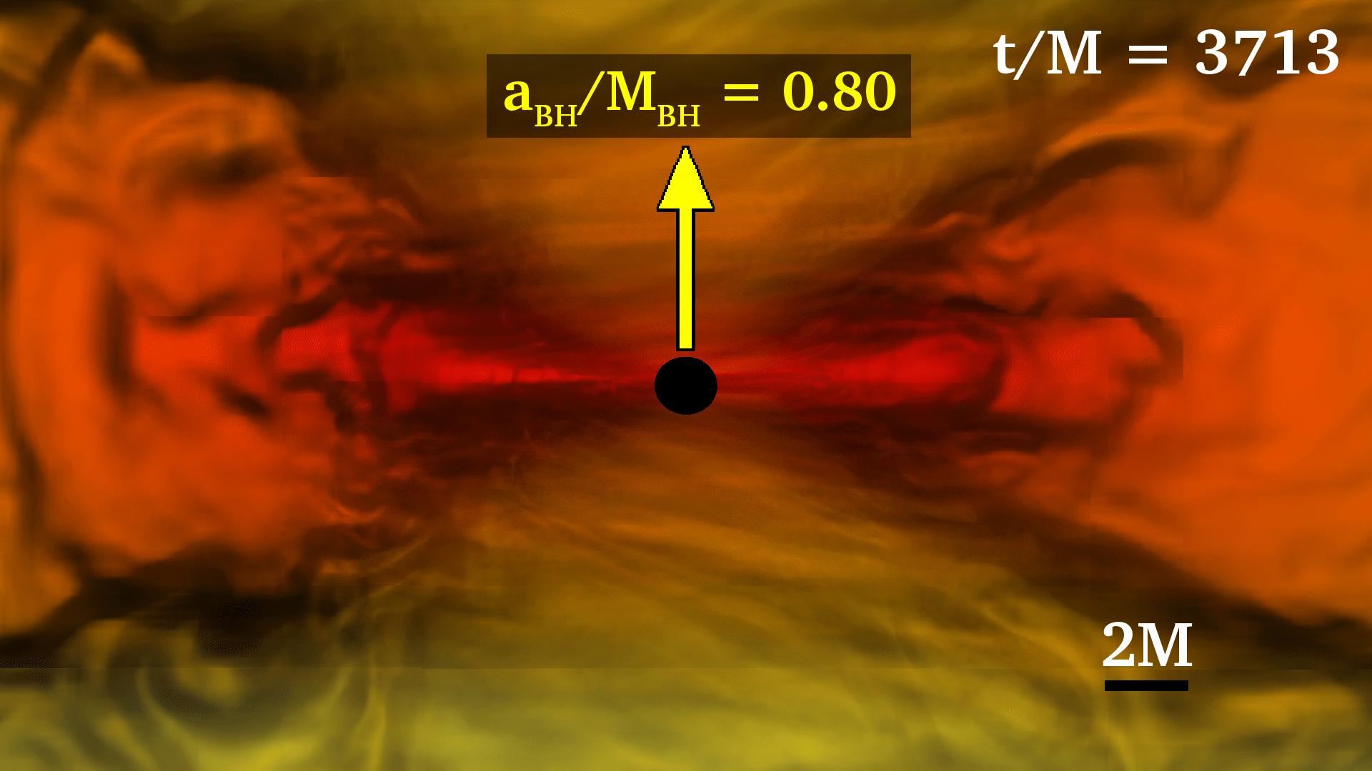
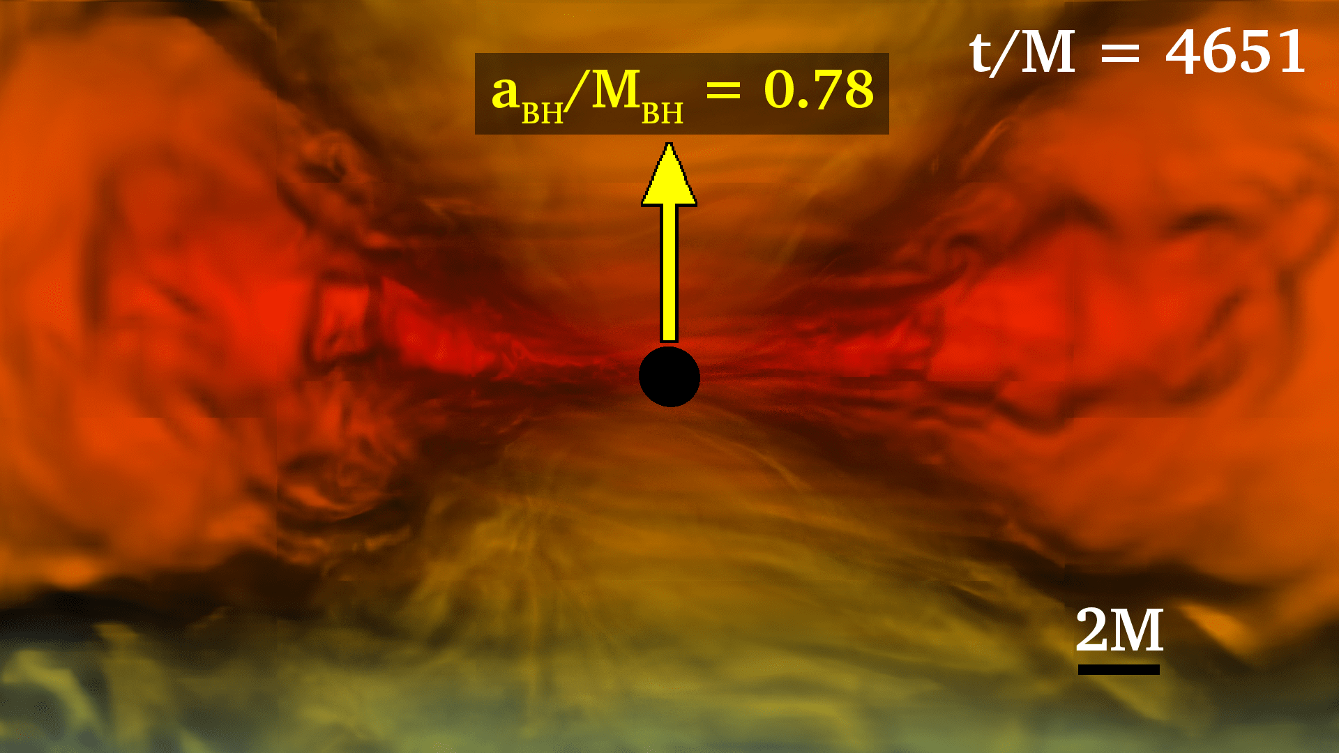
In the two cases, the BH remnant has a mass of with spin parameter equal to either , in Ali-Ali (Eq), or , in the full 3D case. Note that a difference of is approximately at the same level as the accuracy of our numerical simulations. As we state in the previous section, the violation of the conservation of is , though the spins are determined by a local measurement while is determined by a global measurement. Fig. 7 compares their rest-mass profiles following the accretion peaks (see also the fourth row in Fig. 1). We observe that although the fractions of the total rest-mass outside the BH horizon are roughly the same (see Table 1), the accretion disk in the full 3D case is a factor of denser than in Ali-Ali (Eq). Fig. 8 shows the BH + disk remnant near the end of the simulations. Notice that in Ali-Ali, matter tends to pile up around the orbital plane and closer to the BH, while in Ali-Ali (Eq), it is concentrated further out in the bulk of the disk.
During the HMNS collapse, the inner core, which contains most of the magnetic energy , is promptly swallowed by the BH, and hence in the exterior quickly decreases by roughly one order of magnitude in only , and then it slightly decreases as the accretion proceeds reaching a value of (see Fig. 5). As shown in the inset of Fig. 5, following BH formation, the rms value of the poloidal magnetic field is , and remains roughly constant. Similar behavior is observed in the toroidal component.
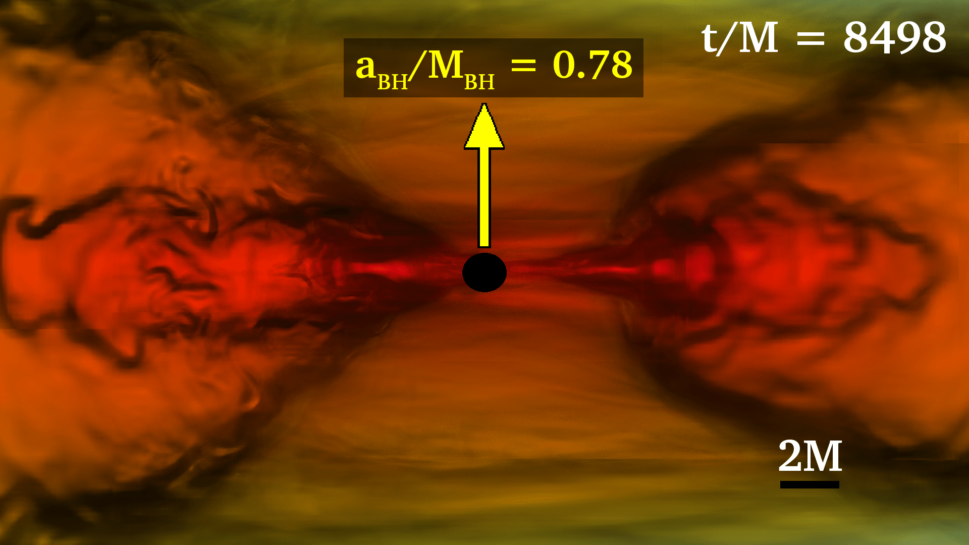
Following the HMNS collapse, the BH remnant is immersed in a heavy-loaded environment: material ejected during the merger or radially blown out during the HMNS epoch begins to rain down. However, magnetic winding begins to build up magnetic pressure above the BH poles until eventually it is large enough to balance the ram pressure of the fall-back material. By , the magnetic pressure above the BH poles stops the inflow. Simultaneously, field lines get wound into a helical structure. We observe that, as displayed in third and fourth rows in Fig. 1, the field lines in the Ali-Ali case are already tightly wound in regions above the BH that extend to heights , where is the coordinate radius of the apparent horizon of the BH, while in the Ali-Ali (Eq) case the magnetic winding is still underway. As the accretion proceeds, the atmosphere becomes thinner and hence magnetically-dominated regions (force-free regions where ) above the BH progressively expand (see top panels in Fig. 9). Once , the magnetic pressure above the BH poles is enough to overcome the ram pressure, and a magnetically-sustained outflow is launched. By , unbound material with a Lorentz factor of (see Table 1) expands beyond heights above the BH. Therefore, we conclude that at about following the gravitational radiation peak, an incipient jet is launched (see bottom panels in Fig. 1). We note that, in the full 3D evolution there is an “apparent” delay in the emergence of the jet, which is launched only earlier than in the equatorial case, though its funnel walls were formed earlier. This delay is likely due to its denser accretion disk that requires longer evolution time for the emptying of the funnel. Nevertheless, field lines are more tightly collimated in the full 3D case (see top panels in Fig. 9). We estimate a funnel opening angle of in Ali-Ali, and a in the equatorial case (see also Ruiz et al. 2019).
| Model | ||||||||||||||||
|---|---|---|---|---|---|---|---|---|---|---|---|---|---|---|---|---|
| Ali-Ali (Eq)∗ | 11.2 | 25.0 | 62 | 0.78 | 2.71 | 138.5 | 0.04 | 1.26 | ||||||||
| Ali-Ali | 11.1 | 23.7 | 62 | 0.80 | 2.86 | 143.9 | 0.05 | 1.29 | ||||||||
| Ali-Per | 11.7 | 41.9 | 70 | 0.78 | 2.47 | 150.4 | 0.02 | 1.24 | ||||||||
| Per-Per | 11.2 | 76.5 | 104 | 0.78 | 2.56 | 144.3 | 0.001 | [N/A] | [N/A] | [N/A] |
∗ Case treated previously in Ruiz et al. 2019, and denoted as Msp0.36.
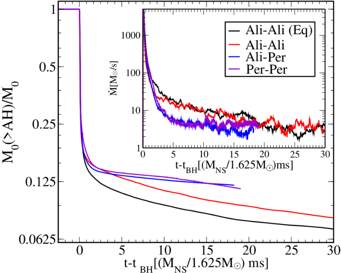
The incipient jet leads to an outgoing EM Poynting luminosity of (see Fig. 10) that is consistent with typical sGRB luminosities Ajello et al. 2019, and has an efficiency of (see Table 1). Similar values were reported in GRMHD simulations of BH immersed in a magnetized accretion disk with similar spins (see e.g. Eq. 3 in McKinney 2005). Near the end of our simulations, the ratio , which equals the maximum achievable Lorentz factor for Poynting-dominated jets Vlahakis and Königl 2003, reaches values larger than above the BH poles (see top panel in Fig. 9). Therefore, as it has been pointed out in Paschalidis et al. 2015a, the mildly relativistic magnetically-driven outflow found in our simulations may be accelerated to Lorentz factors , values required in sGRB phenomenology. Also, notice that the EM luminosity is also roughly consistent with the theoretical expectation from the BZ mechanism (see Eq. 5 in Ruiz et al. 2019). as well as with the “universal model” common to all BH + disk systems formed through the merger or collapse of compact objects Shapiro 2017.
As displayed in the inset of Fig. 7, by , begins to settle down, and gradually decays afterwards. Once the magnetically-driven outflow is launched, we estimate that the lifetime of the disk (fuel of the jet) in both case is (see Table 1), which is entirely consistent with the lifetime of sGRBs Kann et al. 2011.

In addition to the EM outgoing luminosity, NSNS mergers can also give rise to detectable kilonovae if the mass ejecta following the merger is larger than (see e.g. Metzger and Berger 2012; Metzger 2017). The inset in Fig. 10 shows the history of the rest-mass fraction of the escaping matter following the NSNS merger. The material ejected in Ali-Ali (Eq) is , while in Ali-Ali is . So, Ali-Ali cases may lead to kilonovae that can be potentially observed by current or planned telescopes Metzger and Berger 2012.
The above results show that in a timescale of , there are no significant differences between 3D evolutions and those in which symmetry across the orbital plane is imposed. In both cases, the BH + disk remnant launches a magnetically-driven jet. We do not find any evidence of additional magnetic instabilities that can be triggered in full 3D evolutions (e.g. poloidal field instability) as have been previously suggested in Braithwaite and Spruit 2004; Ciolfi and Rezzolla 2012; Ciolfi et al. 2011. Notice that the resistive GRMHD studies reported in Palenzuela et al. 2013 that focus on EM counterparts during the late inspiral and merger epoch of NSNSs, do not observe such instabilities either during an evolution time of , which exceeds the instability growth (Alfvén time) of .
III.2 One aligned and one perpendicular magnetic field
Fig. 2 summarizes the evolution of the rest-mass density along with the magnetic field lines, and fluid velocities, of the Ali-Per case. As in the completely aligned cases, the magnetic field does not play a significant role during the inspiral epoch (see inset in Fig 4). The field lines threading the bulk of each star are simply advected. However, we note that, as the stars approach each other, the field lines connecting them are stretched and wound and, as the coordinate separation decreases, a strong toroidal magnetic field component joining the bulk of the stars emerges.
As displayed in the second panel of Fig. 2, the stars touch at each other for the first time at , and merger roughly later than in the Ali-Ali case (see Table 1), forming a double central core that, after , merges and forms a transient HMNS immersed in a low-density cloud of matter.


During the first , magnetic instabilities amplify the magnetic energy by a factor of , which is slightly larger than in the Ali-Ali cases (see Fig. 5), and, afterward by a factor of during the next until the catastrophic HMNS collapse. Once the HMNS settles down into a quasistationary state (see third panel in Fig. 2), we find that, as in Ali-Ali cases, the quality factor is and fits within the star. However, we note that in this case is , a value slightly smaller than those in Ali-Ali cases (see Table 1), though it is still consistent with those typically produced by turbulent magnetic viscosity Kiuchi et al. 2018. Magnetic braking and magnetic turbulence bring the central region of the HMNS into uniform rotation. The star collapses to a BH at . The BH has a mass of and spin , roughly the same values as those in the Ali-Ali cases (see Table 1).
We note the lifetime of the HMNS remnant in Ali-Per is about longer than in Ali-Ali cases (see Table 1). This delay is likely due to a longer viscous timescale : the smaller the viscosity parameter the longer the time needed by turbulent viscosity to damp differential rotation (see Eq. 3). Moreover, note that, following Sun et al. 2019, the Shakura–Sunyaev parameter can be approximated as , where and are the magnetic field components along the radial and azimuthal directions. So, the induced-magnetic stresses that transport angular momentum outward through the HMNS depend only on the magnitude of the azimuthal and radial components of the magnetic field. As in Ali-Ali and Ali-Per the magnitudes of the poloidal and toroidal magnetic components are similar (see inset in Fig. 5), but the magnetic stresses are smaller in Ali-Per than Ali-Ali because the magnetic field component along the orbital angular momentum prior to merger is smaller (see first row in Fig. 1 and top panel in Fig. 2). Thus, it is expected then that in the Ali-Per case the HMNS collapses later, as we found.
Following the collapse of the HMNS, magnetic winding drives the field lines into a helical funnel (see fourth panel in Fig. 2), and starts to build magnetic pressure above the BH poles. By , a magnetically-sustained outflow (see fifth panel in Fig. 2), with a Lorentz factor of (see Table 1), is launched. In this case, the time-delay between BH formation and jet launching is about larger than in the Ali-Ali cases, likely due to a denser environment: the accretion disk in Ali-Per is denser than that in Ali-Ali (see Table 1), and so it takes longer for the magnetic field to overcome the inertia of the ambient matter (see second and the third panels of Fig. 8). As the strength of the magnetic field does not increase following the BH formation (see inset in Fig. 5), magnetic-dominated regions () above the BH poles appear only after accretion empties the funnel. However, the accretion rate is smaller in Ali-Per than Ali-Ali (see Table 1), and hence the BH + disk remnant in the first case requires a longer time for the jet to emerge. This explains why the ratio in Ali-Per at the end of the simulation is smaller than that in Ali-Ali (see right top and left bottom panels in Fig. 9), though the funnel opening angle is similar ().
The incipient jet leads to an outgoing EM Poynting luminosity of (see Fig. 10) consistent with typical sGRBs. Also, as displayed in the inset of Fig. 7, by , begins to settle down. We estimate the lifetime of the accretion disk to be (see Table 1), implying that the fuel of the jet (the disk) will be exhausted on a time scale consistent with the duration of sGRBs Ajello et al. 2019. It has an efficiency of , roughly the same as that in Ali-Ali (see Table 1). As before, the incipient jet is consistent with the BZ mechanism for launching jet and its Poynting luminosity.
We also find that the ejecta following the NSNS merger is (see inset in Fig. 10), marginally below the detection threshold. Thus, in contrast to the Ali-Ali cases, Ali-Per may not give rise to a detectable kilonova by current or planned telescopes Metzger and Berger 2012. The toroidal magnetic field component formed before the merger tends to trap the outgoing material; fluid elements with a positive radial velocity can become more easily unbound if they do not have to overcome large transverse magnetic stresses arising from the toroidal stretching of field lines. So, magnetic field distributions with a larger poloidal component along the orbital angular momentum of the system lead to a larger ejecta.
The above results show that a change in the initial aligned, poloidal field content has a strong impact on the physical properties of the incipient jet, the magnetically-driven outflow, and hence the likelihood of an observable counterpart kilonova.

III.3 Both perpendicular magnetic fields
Fig. 3 summarizes the evolution of the binary in which the dipole magnetic moment in the two stars is perpendicular to the direction of the total orbital angular momentum of the system (see top left panel). The stars merge at , roughly at the same time as in the Ali-Ali case (see Table 1), forming a HMNS. We note that this transient is the more oblate remnant star of the cases in Table 1, though the central angular velocity is similar in all of them (see Fig. 6).
Following the NSNS merger, and during the next , which approximately corresponds to one Alfvén time (see section IV B in Kiuchi et al. 2018), the magnetic energy is exponentially amplified from to (similar amplification factor was observed in Ali-Per). During this period, the poloidal magnetic field peaks at about , the largest magnetic field strength of the all full 3D cases (see inset of Fig. 5). Following this amplification period, and in contrast to the other cases, the instability saturates more quickly and dies way. The poloidal magnetic field component then decays and relaxes to , its original strength just before the NSNS merger. Similar behavior is observed in the toroidal component. Magnetic winding ceases to enhance the toroidal component once the angular velocity becomes nearly constant in the central core of the HMNS (see right panel of Fig. 6). Similar behavior was found in axisymmetric simulations of highly spinning NSs reported in Duez et al. 2006, where the stellar radius is resolved by grid points, a resolution factor of higher than in our case.
Once the HMNS settles down, we find that is only resolved by grid points, and hence it is at most marginally resolved. By , the viscosity parameter is (see Table 1 for a comparison with the other cases). Although we observe evidence of magnetic turbulence, it may not be fully developed.
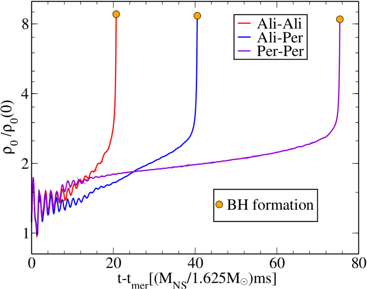
Fig. 11 shows the evolution of the maximum value of the rest-mass density , normalized to its initial value for cases in Table 1. Note that this quantity coincides with the central value of the rest-mass density of the HMNS after . During the first , the dynamics of in cases Ali-Ali and Per-Per is fairly similar. Consistent with magnetic braking (see section IV B in Kiuchi et al. 2018), angular momentum is transferred from the inner to the outer layers of the HMNS. It forms a massive central core with a central rest-mass density surrounded by a cloud of matter (see second panel in Fig. 3). Afterwards, and in contrast to in Ali-Ali that speedily increases, the central density of Ali-Per slowly increases for the next until , where the catastrophic collapse is triggered. This is a time span roughly consistent with the viscous timescale (see Sec. III.2). During this period, the central core shrinks , while the cloud of matter expands by (see forth panel in Fig. 3). Moreover, after (see right panel of Fig. 6), magnetic viscosity has damped the differential rotation in the central core . Here is the central period of the transient HMNS.
As magnetic turbulence may be suppressed by numerical diffusion, we also probe the effect of the resolution on . We rerun the Per-Per case with a resolution factor of higher than before, the highest factor we can afford with the finite computational resources at our disposal. We find that the values of the viscosity parameter within the HMNS turn out to be roughly insensitive to this change in the resolution.
By , the collapse is triggered (see Fig. 11). In the high resolution case, we found that the collapse is triggered roughly later than before. The sensitivity of the collapse time for HMNSs to the magnetic field is physical and has been observed previously (see e.g. Giacomazzo et al. 2011). Its dependence on resolution, even in purely hydrodynamic simulations, has been noted as well (see e.g. Paschalidis et al. 2015b; East et al. 2016). The HMNS collapses to a BH with mass and spin parameter . Similar values were found in all the previous cases (see Table 1).
Following collapse, the magnetic energy decreases even further (see the inset in Fig. 5). After , near to the end of the simulation . We also note that, following the accretion peak, the rms value of the magnetic field in regions directly above the pole is (see Table 1) and remains roughly constant until the end of the simulation.
As displayed in Fig. 7, following the accretion peak, the BH remnant is immersed in an accretion disk with a rest-mass of the total initial rest-mass of the system, a value slightly smaller than the one in the Ali-Per case (see Table 1). The inset of Fig. 7 shows that by the accretion rate begins to settle down, and then gradually decays thereafter. We estimate that the disk will be accreted in . Notice that this timescale is nearly the same as that in the Ali-Ali case (see Table 1), which may indicate that the accretion in Per-Per is also driven by magnetic stresses in the bulk of the disk.
Fig. 8 displays the final configuration of the BH + disk remnant. We note that even after , there is still a dense cloud of fall-back material raining down into the BH remnant. By this time, we do not observe magnetically dominant force-free regions with . As is shown in the bottom left panel of Fig. 9, near to the end of the simulation, we find that this ratio is above the BH poles. We do not find any evidences of an outflow or a large-scale magnetic field collimation (see panel fifth and sixth in Fig. 3). This result is consistent with the GRMHD simulations of NSNS mergers undergoing prompt collapse in Ruiz and Shapiro 2017, which suggest that there is a threshold value of the magnetic energy () below which the BH + disk remnant does not launch a magnetically-supported jet. Finally, the material ejected following the merger is (see inset in Fig. 10), and hence it is unlikely to produce any detectable EM counterpart.
These results suggest that the lack of a large-scale, aligned poloidal field component in the initial system may suppress detectable EM counterparts, such as a magnetically-supported jets or ejecta that can give rise to GRBs or detectable kilonovae.
III.4 Distinguishability of the gravitational waves
By we notice that, in all cases listed in Table 1, the HMNS remnant has reached a quasiaxisymmetric configuration and, as shown in Fig. 4, no longer emits significant gravitational radiation. This time corresponds to a frequency of , near to the edge of the aLIGO high frequency band Shoemaker. So, for frequencies , we probe if our different seed magnetic field configurations are distinguishable by their gravitational waveforms. Fig. 12 shows the gravitational-wave power spectrum of the dominant mode at a source distance of for all the full 3D cases listed in Table 1, along with the aLIGO noise curve of the ZERODETHIGHP configuration Shoemaker. Dashed lines displays the Newtonian prediction Cutler and Flanagan 1994, while the vertical blue line marks the dominant GW frequency of NSNS configurations at the start of the simulations. Note that the spectral features of the waveforms are roughly the same.
We also compute the match function Allen et al. 2012,
| (4) |
between two given waveforms. The maximization is taken over a large set of phase shifts and time shifts . Here denotes the standard noise-weighted inner product (see Appendix C in Allen et al. 2012)
| (5) |
where , is the Fourier transform of the strain amplitude of the dominant mode , and is the power spectral density of the aLIGO noise. Using the aLIGO configuration ZERODETHIGHP, we find that between the waveforms of Ali-Ali and Ali-Per, between the waveforms of Ali-Ali and Per-Per, and between the waveforms of Ali-Per and Per-Per. These results imply that the GWs of Ali-Ali and Per-Per will be potentially distinguishable for a signal-to-noise ratio , while in the other cases, they can be potentially distinguished with a signal-to-noise ratio Chatziioannou et al. 2017; Harry and Hinderer 2018. Note that the first BHBH gravitational wave event was observed with a signal-to-noise ratio of Abbott and et al. 2016, while GW170817 was detected with signal-to-noise ratio of Abbott et al. 2017a. For the numbers quoted above we used the full waveform at the same resolution to compute the match numbers. On the other hand, if one focuses in the postmerger epoch alone (i.e. and a distance of 50 Mpc) the match numbers reduce significantly due to the small signal power above the aLIGO sensitivity level, and distinguishability is lost. However, at smaller distances (e.g. 10 Mpc) distinguishability may again be possible. Our results suggest then that, although in principle, aLIGO may be able to distinguish waveforms arising from different magnetic field configurations, that would practically be very difficult. Future detectors will have better chances to detect magnetic field orientiation effects.
IV Summary and Conclusions
The merger of a binary neutron stars is likely to be the progenitor of the coincident gravitational wave event GW170817 with EM counterparts across the spectrum. It is the likely progenitor of an sGRB (event GRB170817A Abbott et al. 2017b). Such a sGRB counterpart was originally proposed in Paczynski 1986; Eichler et al. 1989; Narayan et al. 1992, and recently demonstrated by self-consistent GRMHD simulations of binary neutron star mergers whose remnant undergoes delayed collapse in Ruiz et al. 2018a; Ruiz and Shapiro 2017. These multimessenger signals have been used to impose some constraints on the physical properties of a neutron star (see e.g. Margalit and Metzger 2017; Shibata et al. 2017; Ruiz et al. 2018b; Rezzolla et al. 2018; Most et al. 2018; Abbott et al. 2017a; Abbott et al. 2018; Radice et al. 2018; Bauswein et al. 2017 and references therein), such as the maximum mass of a spherical star, tidal deformability, equation of state, radius of a neutron star, etc.
To solidify the role of binary neutron star mergers as multimessenger sources, we studied in this paper the impact of different orientations of seed magnetic field configurations. We focused on the emergence of a magnetically-driven jet and the ejecta that may give rise to a kilonova detectable by current telescopes, such as the Large Synoptic Survey Telescope Shibata et al. 2017; Rosswog 2005. We considered spinning binary neutron stars initially on a quasicircular orbit undergoing merger and delayed collapse to a BH. The binaries consisted of two identical polytropes with spin aligned along the direction of the total orbital angular momentum of the system . Each star is initially threaded by an interior and exterior magnetic field resembling that of pulsars, and whose dipole moment is either aligned or perpendicular to . For comparison purposes, we also considered the binary evolution in which in both stars is aligned along but where we imposed symmetry across the orbital plane (equatorial symmetry), to calibrate what is done in numerous simulations.
We found that following merger, in all cases listed in Table 1, magnetic braking in the bulk of the HMNS remnant induces the formation of a nearly uniformly rotating central core immersed in a low-density Keplerian cloud of matter that eventually collapses to a BH. Depending on the initial poloidal field content along , the HMNS collapses in a timescale ranging between , when in both stars is aligned along , to , when it is perpendicular in both of them. Nevertheless, the mass [] and the spin parameter [] of the BH remnant, as well as the rest-mass of the accretion disk [], are roughly independent of the initial magnetic field orientation.
We noticed that the final magnetic energy is also highly affected by the content of the large-scale, aligned poloidal magnetic field prior to merger. As shown in Fig. 5, the larger the component, the larger the final magnetic energy. Consistent with the GRMHD simulations of binary neutron star mergers undergoing prompt collapse in Ruiz and Shapiro 2017, which suggest that there is a threshold value of the magnetic energy below which the BH + disk remnant does not launch an incipient jet, we found that only in the cases in which the magnetic energy becomes larger than , where is the ADM mass of the system, does a magnetically-supported jet emerge. The lifetime [] and Poynting luminosities [erg/s] of the jet are consistent with typical short gamma ray bursts, as well as with the Blandford–Znajek mechanism for launching jets. Moreover, as shown in Fig.1, symmetries do not play a significant role in the binary evolution: the final outcome in the equatorial case is roughly the same as that in the full 3D case. We also noticed that the magnetic field configuration does have a strong affect on the material ejected following the merger. We found that, only in cases where in both stars is aligned with , the computed ejecta is , the value required to give rise to a detectable kilonova Shibata et al. 2017; Rosswog 2005. In the case where in one star is aligned with and in the other star perpendicular to it, the ejecta is marginally below the detectability threshold value, and hence the kilonova may not be detected by current or planned telescopes. In the case where in both stars is perpendicular to , the ejecta is negligible.
Our preliminary results indicate that the binary neutron star merger models without magnetic fields used to explain the early part of the radioactively powered kilonova signal (blue luminosity) linked to GW170817 may overestimate the amount of escaping matter and, therefore, its corresponding luminosity. Higher resolution studies involving more general magnetic configurations may be required to obtain solid estimates.
We also probed whether different seed magnetic field orientations could be distinguishable by aLIGO. For that we computed the match function (see Eq. 4). We find that between the waveforms of Ali-Ali and Ali-Per, between the waveforms of Ali-Ali and Per-Per, and between the waveforms of Ali-Per and Per-Per. These results imply that, the GWs of Ali-Ali and Per-Per will be distinguishable for a signal-to-noise ratio , while in the other cases, they can be distinguished with a signal-to-noise ratio . Hence current detectors may, in principle, be able to distinguish different magnetic configurations.
Acknowledgements.
We thank the Illinois Relativity Group REU team, G. Liu, K. Nelli, M. N.T Nguyen, and S. Qunell for assistance with some of the visualizations. This work was supported by NSF grant PHY-1662211 and NASA grant 80NSSC17K0070 to the University of Illinois at Urbana-Champaign. This work made use of the Extreme Science and Engineering Discovery Environment (XSEDE), which is supported by National Science Foundation grant number TG-MCA99S008. This research is part of the Blue Waters sustained-petascale computing project, which is supported by the National Science Foundation (awards OCI-0725070 and ACI-1238993) and the State of Illinois. Blue Waters is a joint effort of the University of Illinois at Urbana-Champaign and its National Center for Supercomputing Applications. Re-sources supporting this work were also provided by the NASA High-End Computing (HEC) Program through the NASA Advanced Supercomputing (NAS) Division at Ames Research Center.References
- Paczynski (1986) B. Paczynski, Astrophys. J. 308, L43 (1986).
- Eichler et al. (1989) D. Eichler, M. Livio, T. Piran, and D. N. Schramm, Nature (London) 340, 126 (1989).
- Narayan et al. (1992) R. Narayan, B. Paczynski, and T. Piran, Astrophys. J. Letters 395, L83 (1992).
- Tanvir et al. (2013) N. R. Tanvir et al., Nature 500, 547 (2013).
- Berger et al. (2013) E. Berger, W. Fong, and R. Chornock, Astrophys. J. 774, L23 (2013).
- Paschalidis et al. (2015a) V. Paschalidis, M. Ruiz, and S. L. Shapiro, Astrophys. J. 806, L14 (2015a), arXiv:1410.7392 [astro-ph.HE] .
- Ruiz et al. (2018a) M. Ruiz, S. L. Shapiro, and A. Tsokaros, (2018a), arXiv:1810.08618 [astro-ph.HE] .
- Ruiz et al. (2016) M. Ruiz, R. N. Lang, V. Paschalidis, and S. L. Shapiro, Astrophys. J. 824, L6 (2016).
- Ruiz and Shapiro (2017) M. Ruiz and S. L. Shapiro, Phys. Rev. D96, 084063 (2017), arXiv:1709.00414 [astro-ph.HE] .
- Abbott et al. (2017a) B. P. Abbott et al. (Virgo, LIGO Scientific), Phys. Rev. Lett. 119, 161101 (2017a), arXiv:1710.05832 [gr-qc] .
- Abbott et al. (2017b) B. P. Abbott et al. (Virgo, Fermi-GBM, INTEGRAL, LIGO Scientific), Astrophys. J. 848, L13 (2017b), arXiv:1710.05834 [astro-ph.HE] .
- Valenti et al. (2017) S. Valenti, D. J. Sand, S. Yang, E. Cappellaro, L. Tartaglia, A. Corsi, S. W. Jha, D. E. Reichart, J. Haislip, and V. Kouprianov, Astrophys. J. 848, L24 (2017), arXiv:1710.05854 [astro-ph.HE] .
- Özel and Freire (2016) F. Özel and P. Freire, Ann. Rev. Astron. Astrophys. 54, 401 (2016), arXiv:1603.02698 [astro-ph.HE] .
- Lattimer and Prakash (2016) J. M. Lattimer and M. Prakash, Phys. Rept. 621, 127 (2016), arXiv:1512.07820 [astro-ph.SR] .
- Bogdanov et al. (2019a) S. Bogdanov et al., Astrophys. J. 887, L26 (2019a), arXiv:1912.05707 [astro-ph.HE] .
- Bogdanov et al. (2019b) S. Bogdanov et al., Astrophys. J. 887, L25 (2019b), arXiv:1912.05706 [astro-ph.HE] .
- Foucart et al. (2018) F. Foucart, T. Hinderer, and S. Nissanke, Phys. Rev. D98, 081501 (2018), arXiv:1807.00011 [astro-ph.HE] .
- Thompson et al. (2019) T. A. Thompson, C. S. Kochanek, K. Z. Stanek, C. Badenes, R. S. Post, T. Jayasinghe, D. W. Latham, A. Bieryla, G. A. Esquerdo, P. Berlind, M. L. Calkins, J. Tayar, L. Lindegren, J. A. Johnson, T. W.-S. Holoien, K. Auchettl, and K. Covey, Science 366, 637 (2019), https://science.sciencemag.org/content/366/6465/637.full.pdf .
- Yang et al. (2018) H. Yang, W. E. East, and L. Lehner, Astrophys. J. 856, 110 (2018), arXiv:1710.05891 [gr-qc] .
- Bhat et al. (2016) P. N. Bhat et al., Astrophys. J. Suppl. 223, 28 (2016), arXiv:1603.07612 [astro-ph.HE] .
- Lien et al. (2016) A. Lien et al., Astrophys. J. 829, 7 (2016), arXiv:1606.01956 [astro-ph.HE] .
- Svinkin et al. (2016) D. S. Svinkin, D. D. Frederiks, R. L. Aptekar, S. V. Golenetskii, V. D. Pal’shin, P. P. Oleynik, A. E. Tsvetkova, M. V. Ulanov, T. L. Cline, and K. Hurley, Astrophys. J. Suppl. 224, 10 (2016), arXiv:1603.06832 [astro-ph.HE] .
- Ajello et al. (2019) M. Ajello et al., Astrophys. J. 878, 52 (2019), arXiv:1906.11403 [astro-ph.HE] .
- Blandford and Znajek (1977a) R. D. Blandford and R. L. Znajek, Mon. Not. Roy. Astron. Soc. 179, 433 (1977a).
- Beckwith et al. (2008) K. Beckwith, J. F. Hawley, and J. H. Krolik, Astrophys. J. 678, 1180 (2008).
- Beckwith et al. (2009) K. Beckwith, J. F. Hawley, and J. H. Krolik, Astrophys. J. 707, 428 (2009), arXiv:0906.2784 [astro-ph.HE] .
- Etienne et al. (2012) Z. B. Etienne, Y. T. Liu, V. Paschalidis, and S. L. Shapiro, Phys.Rev. D85, 064029 (2012).
- Ruiz et al. (2019) M. Ruiz, A. Tsokaros, V. Paschalidis, and S. L. Shapiro, Phys. Rev. D99, 084032 (2019), arXiv:1902.08636 [astro-ph.HE] .
- Totani (2013) T. Totani, Pub. Astron. Soc. Jpn. 65, L12 (2013).
- Paschalidis and Ruiz (2019) V. Paschalidis and M. Ruiz, Phys. Rev. D100, 043001 (2019), arXiv:1808.04822 [astro-ph.HE] .
- Kiuchi et al. (2014) K. Kiuchi, K. Kyutoku, Y. Sekiguchi, M. Shibata, and T. Wada, Phys.Rev. D90, 041502 (2014).
- Kawamura et al. (2016) T. Kawamura, B. Giacomazzo, W. Kastaun, R. Ciolfi, A. Endrizzi, L. Baiotti, and R. Perna, Phys. Rev. D94, 064012 (2016), arXiv:1607.01791 [astro-ph.HE] .
- Ciolfi et al. (2017) R. Ciolfi, W. Kastaun, B. Giacomazzo, A. Endrizzi, D. M. Siegel, and R. Perna, Phys. Rev. D95, 063016 (2017), arXiv:1701.08738 [astro-ph.HE] .
- Paschalidis (2017) V. Paschalidis, Class. Quant. Grav. 34, 084002 (2017).
- Markey and Tayler (1973) P. Markey and R. J. Tayler, mnras 163, 77 (1973).
- Wright (1973) G. A. E. Wright, mnras 162, 339 (1973).
- Braithwaite and Spruit (2004) J. Braithwaite and H. C. Spruit, Nature 431, 819 (2004), arXiv:astro-ph/0502043 [astro-ph] .
- Ciolfi and Rezzolla (2012) R. Ciolfi and L. Rezzolla, Astrophys. J. 760, 1 (2012), arXiv:1206.6604 [astro-ph.SR] .
- Ciolfi et al. (2011) R. Ciolfi, S. K. Lander, G. M. Manca, and L. Rezzolla, Astrophys. J. 736, L6 (2011), arXiv:1105.3971 [gr-qc] .
- Moffatt (1978) H. K. Moffatt, Magnetic field generation in electrically conducting fluids (1978).
- Tsokaros et al. (2018) A. Tsokaros, K. Uryu, M. Ruiz, and S. L. Shapiro, Phys. Rev. D98, 124019 (2018), arXiv:1809.08237 [gr-qc] .
- Blandford and Znajek (1977b) R. D. Blandford and R. L. Znajek, mnras 179, 433 (1977b).
- Shibata et al. (2017) M. Shibata, S. Fujibayashi, K. Hotokezaka, K. Kiuchi, K. Kyutoku, Y. Sekiguchi, and M. Tanaka, Phys. Rev. D96, 123012 (2017), arXiv:1710.07579 [astro-ph.HE] .
- Rosswog (2005) S. Rosswog, Astrophys. J. 634, 1202 (2005).
- Abbott and et al. (2016) B. P. Abbott and et al. (LIGO Scientific Collaboration and Virgo Collaboration), Phys. Rev. Lett. 116, 061102 (2016).
- Etienne et al. (2010) Z. B. Etienne, Y. T. Liu, and S. L. Shapiro, Phys.Rev. D82, 084031 (2010).
- (47) Cactus, “Cactuscode, http://cactuscode.org/,” .
- (48) Carpet, Carpet Code homepage.
- Shibata and Nakamura (1995) M. Shibata and T. Nakamura, Phys. Rev. D 52, 5428 (1995).
- Baumgarte and Shapiro (1999) T. W. Baumgarte and S. L. Shapiro, Phys. Rev. D59, 024007 (1999), arXiv:gr-qc/9810065 [gr-qc] .
- Etienne et al. (2008) Z. B. Etienne, J. A. Faber, Y. T. Liu, S. L. Shapiro, K. Taniguchi, and T. W. Baumgarte, Phys. Rev. D77, 084002 (2008), arXiv:0712.2460 [astro-ph] .
- Baker et al. (2006) J. G. Baker, J. Centrella, D.-I. Choi, M. Koppitz, and J. van Meter, Phys. Rev. D 73, 104002 (2006).
- Duez et al. (2003) M. D. Duez, P. Marronetti, S. L. Shapiro, and T. W. Baumgarte, Phys. Rev. D 67, 024004 (2003).
- Tsokaros et al. (2015) A. Tsokaros, K. Uryū, and L. Rezzolla, Phys. Rev. D91, 104030 (2015), arXiv:1502.05674 [gr-qc] .
- Tsokaros et al. (2016) A. Tsokaros, B. C. Mundim, F. Galeazzi, L. Rezzolla, and K. Uryū, Phys. Rev. D94, 044049 (2016), arXiv:1605.07205 [gr-qc] .
- Kiuchi et al. (2015) K. Kiuchi, P. Cerdá-Durán, K. Kyutoku, Y. Sekiguchi, and M. Shibata, Phys. Rev. D92, 124034 (2015).
- Tsokaros et al. (2019) A. Tsokaros, M. Ruiz, V. Paschalidis, S. L. Shapiro, and K. Uryū, Phys. Rev. D100, 024061 (2019), arXiv:1906.00011 [gr-qc] .
- Ruiz et al. (2008) M. Ruiz, R. Takahashi, M. Alcubierre, and D. Nunez, Gen. Rel. Grav. 40, 2467 (2008).
- Shiokawa et al. (2012) H. Shiokawa, J. C. Dolence, C. F. Gammie, and S. C. Noble, Astrophys. J. 744, 187 (2012), arXiv:1111.0396 [astro-ph.HE] .
- Sano et al. (2004) T. Sano, S.-i. Inutsuka, N. J. Turner, and J. M. Stone, Astrophys. J. 605, 321 (2004), arXiv:astro-ph/0312480 [astro-ph] .
- Penna et al. (2010) R. F. Penna, J. C. McKinney, R. Narayan, A. Tchekhovskoy, R. Shafee, and J. E. McClintock, mnras 408, 752 (2010).
- Gold et al. (2014) R. Gold, V. Paschalidis, Z. B. Etienne, S. L. Shapiro, and H. P. Pfeiffer, Phys.Rev. D89, 064060 (2014), arXiv:1312.0600 [astro-ph.HE] .
- Thornburg (2004) J. Thornburg, Class. Quant. Grav. 21, 743 (2004).
- Dreyer et al. (2003) O. Dreyer, B. Krishnan, D. Shoemaker, and E. Schnetter, Phys. Rev. D 67, 024018 (2003).
- Farris et al. (2010) B. D. Farris, Y. T. Liu, and S. L. Shapiro, Phys.Rev. D81, 084008 (2010).
- Cook et al. (1994) G. B. Cook, S. L. Shapiro, and S. A. Teukolsky, Astrophys. J. 422, 227 (1994).
- Lyford et al. (2003) N. D. Lyford, T. W. Baumgarte, and S. L. Shapiro, Astrophys. J. 583, 410 (2003), gr-qc/0210012 .
- Kiuchi et al. (2018) K. Kiuchi, K. Kyutoku, Y. Sekiguchi, and M. Shibata, Phys. Rev. D97, 124039 (2018), arXiv:1710.01311 [astro-ph.HE] .
- Hawley et al. (2011) J. F. Hawley, X. Guan, and J. H. Krolik, Astrophys. J. 738, 84 (2011), arXiv:1103.5987 [astro-ph.HE] .
- Hawley et al. (2013) J. F. Hawley, S. A. Richers, X. Guan, and J. H. Krolik, Astrophys. J. 772, 102 (2013), arXiv:1306.0243 [astro-ph.IM] .
- Sun et al. (2019) L. Sun, M. Ruiz, and S. L. Shapiro, Phys. Rev. D99, 064057 (2019), arXiv:1812.03176 [astro-ph.HE] .
- Shibata and Uryu (2002) M. Shibata and K. Uryu, Prog. Theor. Phys. 107, 265 (2002), arXiv:gr-qc/0203037 [gr-qc] .
- Shibata and Taniguchi (2006) M. Shibata and K. Taniguchi, Phys. Rev. D73, 064027 (2006), arXiv:astro-ph/0603145 [astro-ph] .
- Kastaun et al. (2016) W. Kastaun, R. Ciolfi, and B. Giacomazzo, Phys. Rev. D94, 044060 (2016), arXiv:1607.02186 [astro-ph.HE] .
- McKinney (2005) J. C. McKinney, Astrophys. J. 630, L5 (2005), arXiv:astro-ph/0506367 [astro-ph] .
- Vlahakis and Königl (2003) N. Vlahakis and A. Königl, “Relativistic Magnetohydrodynamics with Application to Gamma-Ray Burst Outflows. I. Theory and Semianalytic Trans-Alfvénic Solutions,” (2003).
- Shapiro (2017) S. L. Shapiro, Phys. Rev. D95, 101303 (2017), arXiv:1705.04695 [astro-ph.HE] .
- Kann et al. (2011) D. A. Kann et al., Astrophys. J. 734, 96 (2011).
- Metzger and Berger (2012) B. D. Metzger and E. Berger, Astrophys. J. 746, 48 (2012).
- Metzger (2017) B. D. Metzger, Living Rev. Rel. 20, 3 (2017), arXiv:1610.09381 [astro-ph.HE] .
- Palenzuela et al. (2013) C. Palenzuela, L. Lehner, S. L. Liebling, M. Ponce, M. Anderson, D. Neilsen, and P. Motl, Phys. Rev. D88, 043011 (2013), arXiv:1307.7372 [gr-qc] .
- Duez et al. (2006) M. D. Duez, Y. T. Liu, S. L. Shapiro, M. Shibata, and B. C. Stephens, Phys. Rev. D 73, 104015 (2006).
- Giacomazzo et al. (2011) B. Giacomazzo, L. Rezzolla, and L. Baiotti, Phys. Rev. D 83, 044014 (2011).
- Paschalidis et al. (2015b) V. Paschalidis, W. E. East, F. Pretorius, and S. L. Shapiro, Phys. Rev. D 92, 121502 (2015b), arXiv:1510.03432 [astro-ph.HE] .
- East et al. (2016) W. E. East, V. Paschalidis, F. Pretorius, and S. L. Shapiro, Phys. Rev. D 93, 024011 (2016), arXiv:1511.01093 [astro-ph.HE] .
- (86) D. Shoemaker, LIGO Report No. LIGO-T0900288-v2, 2009, the high-power detuned model used in this paper is given in the data file ZERO_DET_HIGH_Pxf.TXT.
- Cutler and Flanagan (1994) C. Cutler and E. E. Flanagan, Phys. Rev. D49, 2658 (1994).
- Allen et al. (2012) B. Allen, W. G. Anderson, P. R. Brady, D. A. Brown, and J. D. E. Creighton, Phys. Rev. D 85, 122006 (2012).
- Chatziioannou et al. (2017) K. Chatziioannou, A. Klein, N. Yunes, and N. Cornish, Phys. Rev. D 95, 104004 (2017).
- Harry and Hinderer (2018) I. Harry and T. Hinderer, Classical and Quantum Gravity 35, 145010 (2018).
- Margalit and Metzger (2017) B. Margalit and B. D. Metzger, Astrophys. J. 850, L19 (2017), arXiv:1710.05938 [astro-ph.HE] .
- Ruiz et al. (2018b) M. Ruiz, S. L. Shapiro, and A. Tsokaros, Phys. Rev. D97, 021501 (2018b), arXiv:1711.00473 [astro-ph.HE] .
- Rezzolla et al. (2018) L. Rezzolla, E. R. Most, and L. R. Weih, Astrophys. J. 852, L25 (2018), [Astrophys. J. Lett.852,L25(2018)], arXiv:1711.00314 [astro-ph.HE] .
- Most et al. (2018) E. R. Most, L. R. Weih, L. Rezzolla, and J. Schaffner-Bielich, Phys. Rev. Lett. 120, 261103 (2018), arXiv:1803.00549 [gr-qc] .
- Abbott et al. (2018) B. P. Abbott et al. (Virgo, LIGO Scientific), (2018), arXiv:1805.11581 [gr-qc] .
- Radice et al. (2018) D. Radice, A. Perego, F. Zappa, and S. Bernuzzi, Astrophys. J. 852, L29 (2018), arXiv:1711.03647 [astro-ph.HE] .
- Bauswein et al. (2017) A. Bauswein, O. Just, H.-T. Janka, and N. Stergioulas, Astrophys. J. 850, L34 (2017), arXiv:1710.06843 [astro-ph.HE] .