Intelligent Reflecting Surface Assisted Secure Wireless Communications with Multiple-Transmit and Multiple-Receive Antennas

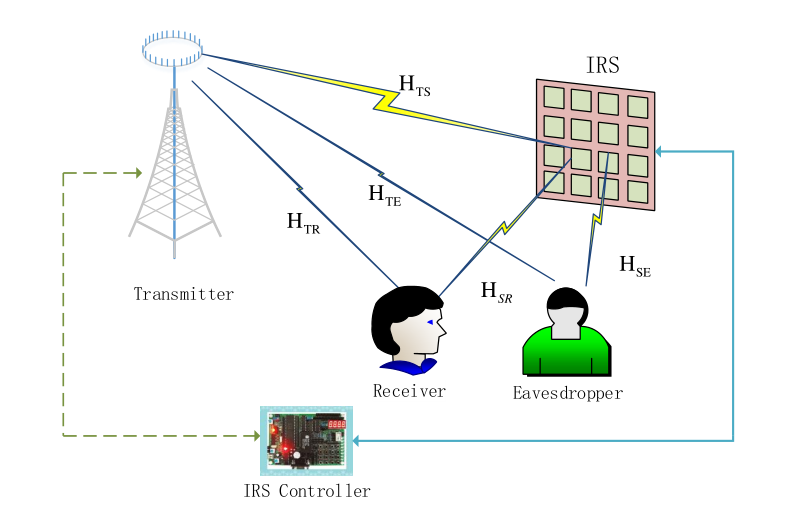
Consider the IRS assisted MIMOME system, as shown in Fig. 1, where an AP equipped with $N_{T}$ antennas serves a legitimate user at the present of an eavesdropper. Both the legitimate user and the eavesdropper are equipped with multi-antenna and the number of the antennas at these two users are $N_{R}$ and $N_{E}$, respectively. In addition, an IRS composed of $M$ passive elements is installed on a surrounding wall to assist the secure communications between the AP and the legitimate user. The IRS has a smart controller, who has the capability of dynamically adjusting the phase shift of each reflecting element based on the propagation environment learned through periodic sensing [6]. In particular, the IRS controller coordinates the switching between two working modes, i.e., receiving mode for environment sensing (e.g., channel state information (CSI) estimation) and reflecting mode for scattering the incident signals from the AP [26].

Following [27], the phase shift matrix of the IRS can be defined as $\mathbf{\mathbf{\Theta}}=diag(\bm{\theta})\in{{\mathbb{C}}^{M\times M}}$, where $\bm{\theta}=[\theta_{1},\theta_{2},\cdots,\theta_{M}]^{T}\in{{\mathbb{C}}^{M\times 1}}$ and $\theta_{m}\in\bm{\Phi}$ for $1\leq m\leq M$, and $diag(\bullet)$ denotes a diagonal matrix whose diagonal elements are given by the corresponding vector and $\bm{\Phi}$ denotes the set of reflecting coefficients of the IRS. In this paper, two different sets of reflecting coefficients are considered as below.

For our considered system, as [6], the signals that are reflected by the IRS multi-times are ignored due to significant path loss. Therefore, combined with IRS reflecting coefficient model, the signals received at the legitimate user and the eavesdropper can be expressed as

As mentioned earlier, in this paper, we discuss the joint optimization of the transmit covariance matrix at the AP and the reflection coefficients at the IRS to maximize the system secrecy rate subjected to the transmit power constraint at the AP and the reflection coefficient constraint at the IRS. Thus we have the following optimization problem OP1,

In which, C1 characterizes the total transmit power constraint at the AP, C2 defines the positive semi-define constraint on transmit covariance matrix, and C3 represents the IRS reflecting coefficient model. It is obvious that OP1 is a non-convex nonlinear programming with non-convex objective function and the uni-modular constraint on each reflection coefficient $\theta_{m}$, which makes it difficult to be solved. Therefore, in the sequel, we pursue the suboptimal approach to handle OP1.

In this subsection, we discuss the transmit covariance matrix optimization at the AP for given the reflecting coefficients at the IRS. Hence, we have the following problem OP2,

Herein, given the reflection coefficient matrix $\mathbf{\Theta}$ at the IRS, $\mathbf{G}_{TR}(\mathbf{\Theta})$ and $\mathbf{G}_{TE}(\mathbf{\Theta})$ are simplistically denoted as $\mathbf{G}_{TR}$ and $\mathbf{G}_{TE}$, respectively. One may note that, now, the formulated problem OP2 is the secrecy rate maximization problem for the MIMOME system which has been discussed in [32], [33] and [34], and various algorithms have been proposed therein. In this paper, following [32], the SCA-based suboptimal algorithm is used to handle OP2. And the key point is to obtain a tight concave lower bound of ${R_{sec}}\left({\mathbf{Q}_{s}}\right)$, which can be achieved by retaining the concave part ${R_{R}}\left({\mathbf{Q}_{s}}\right)$ in (10) and linearizing the concave function ${R_{E}}\left({\mathbf{Q}_{s}}\right)$ [35, 36]. That is, at ${\mathbf{\tilde{Q}}}_{s}$, we have the concave approximation of ${R_{sec}}\left({\mathbf{Q}_{s}}\right)$ as follows,

where $\mathbf{W}_{E,{\mathbf{\tilde{Q}}_{s}}}={\mathbf{I}_{N_{E}}}+\frac{1}{\sigma_{E}^{2}}{\mathbf{G}_{TE}}{{\mathbf{\tilde{Q}}}_{s}}\mathbf{G}_{TE}^{H}$. Based on the above approximation and given ${\mathbf{\tilde{Q}}}_{s}$, the problem OP2 can be transformed into the following formulation,

Then this problem is convex and can be easily solved using standard interior-point methods [32]. That is, the Karush¨CKuhn¨CTucker (KKT) conditions [37] for the above convex approximation problem are, namely,

Herein, ${\mathbf{W}_{R}}={\mathbf{I}_{N_{R}}}+\frac{1}{\sigma_{R}^{2}}{\mathbf{G}_{TR}}{\mathbf{Q}_{s}}\mathbf{G}_{TR}^{H}$. $\lambda\geq 0$ and $\mathbf{Z}\succcurlyeq 0$ are the dual variables associated with the transmission power constraint and the positive semi-definite constraint on the $\mathbf{Q}_{s}$, respectively. Correspondingly, the Lagrangian function of (12) can be written as

Since problem (12) is convex and satisfies the Slater’s condition, the duality gap is zero between (12) and its dual problem. Thus, the optimal solution of (12) can be determined via solving the following Lagrange dual problem

Herein,

To sum up, we have the SCA based suboptimal algorithm for OP2 which is summarized as the Algorithm 1 as below.

In this subsection, given the transmit covariance matrix $\mathbf{Q}_{s}$ at the AP, the optimization the reflecting coefficient matrix $\mathbf{\Theta}$ at IRS with the continuous model is discussed. Particularly, we have the following problem OP3.

It is obvious that OP3 is a non-convex programming with both non-convex constraints and non-concave objective function, which makes it is difficult to be solved. However, we prove that, given $\left\{{{\theta}_{i}}\right\}_{i=1,i\neq m}^{M}$, the formulated optimization problem with respect to $\theta_{m}$ can be solved with the close-form optimal solution or to have an interval about the optimal solution. Therefore, the alternative optimization approach is used here again to solve OP3, i.e., we alternatively solve OP3 in variable $\theta_{m}$ with given $\theta_{i},i=1,...,M,i\neq m$ until the procedure is converged. The details are illustrated as follows.

1) Objective function transformation: In order to use the alternative optimization approach to solve OP3, we should first make an objective function transformation for OP3. Note that, the relationship of the objective function with $\left\{{\theta_{m}}\right\}_{m=1}^{M}$ is rather implicit. Thus, we rewrite the objective function as an explicit function over $\theta_{m},\forall m$. That is [38],

Herein, let $\mathbf{Q}_{s}={\mathbf{U}_{Q}}{\mathbf{\Sigma}_{Q}}{\mathbf{U}_{Q}^{H}}$ as the eigenvalue decomposition (EVD) of ${\mathbf{Q}_{s}}\succcurlyeq 0$, ${\mathbf{U}_{Q}}\in{{\mathbb{C}}^{{N_{T}}\times{N_{T}}}}$ and ${\mathbf{\Sigma}_{Q}}\in{{\mathbb{C}}^{{N_{T}}\times{N_{T}}}}$ are unitary matrix and diagonal matrix, respectively, and all the diagonal elements in ${\mathbf{\Sigma}_{Q}}$ are non-negative real numbers. Also, in (18), we define ${{\mathbf{H}}_{SR}}=[{{\bm{h}}_{SR,1}},...,{{\bm{h}}_{SR,M}}]$, ${{\mathbf{H}}_{SE}}=[{{\bm{h}}_{SE,1}},...,{{\bm{h}}_{SE,M}}]$ , $\overline{\mathbf{H}}_{TS}=\mathbf{H}_{TS}\mathbf{U}_{Q}\mathbf{\Sigma}_{Q}^{{1}/{2}\;}={{[\overline{\bm{h}}_{TS,1},...,\overline{\bm{h}}_{TR,M}]}^{H}}$, $\overline{\mathbf{H}}_{TR}=\mathbf{H}_{TR}\mathbf{U}_{Q}\mathbf{\Sigma}_{Q}^{{1}/{2}\;}\in{{\mathbb{C}}^{{{N}_{R}}\times{{N}_{T}}}}$, $\overline{\mathbf{H}}_{TE}={{\mathbf{H}}_{TE}}{{\mathbf{U}}_{Q}}\mathbf{\Sigma}_{Q}^{{1}/{2}\;}\in{{\mathbb{C}}^{{{N}_{E}}\times{{N}_{T}}}}$, and ${{\bm{h}}_{SR,m}}\in{{\mathbb{C}}^{{{N}_{R}}\times 1}}$, ${{\bm{h}}_{SE,m}}\in{{\mathbb{C}}^{{{N}_{E}}\times 1}}$, $\overline{\bm{h}}_{TS,m}\in{{\mathbb{C}}^{{{N}_{T}}\times 1}},m=1,2,...M$. Now, $R_{sec}$ is represented in an explicit form of the reflection coefficients $\left\{{\theta_{m}}\right\}_{m=1}^{M}$. Therefore, given $\mathbf{Q}_{s}$ and $\left\{{\theta_{i}}\right\}_{i=1,i\neq m}^{M}$, $R_{sec}$ can be rewritten as a function of $\theta_{m}$ as,

where,

We denote $\hat{\mathbf{H}}_{R}=\overline{\mathbf{H}}_{TR}+\sum\limits_{i=1,i\neq m}^{M}{{{\theta}_{i}}{{\bm{h}}_{SR,i}}\overline{\bm{h}}_{TS,i}^{H}}$, $\hat{\mathbf{H}}_{E}=\overline{\mathbf{H}}_{TE}+\sum\limits_{i=1,i\neq m}^{M}{{{\theta}_{i}}{{\bm{h}}_{SE,i}}\overline{\bm{h}}_{TS,i}^{H}}$, $\tilde{\mathbf{H}}_{R}={{\bm{h}}_{SR,m}}\overline{\bm{h}}_{TS,m}^{H}$ and $\tilde{\mathbf{H}}_{E}={{\bm{h}}_{SE,m}}\overline{\bm{h}}_{TS,m}^{H}$. Since both ${\mathbf{A}}_{R,m}$ and ${\mathbf{A}}_{E,m}$ are the sum of identity matrix and the two positive semi-define matrixes, thus we have $\mathbf{A}_{R,m}\succ 0$, $\mathbf{A}_{E,m}\succ 0$, $rank\left({{\mathbf{A}}_{R,m}}\right)={{N}_{R}}$ and $rank\left({{\mathbf{A}}_{E,m}}\right)={{N}_{E}}$. Moreover, for ${\mathbf{B}}_{R,m}$ and ${\mathbf{B}}_{E,m}$ we have $rank\left({{\mathbf{B}}_{R,m}}\right)\leq\\ rank\left({{\bm{h}}_{SR,m}}\overline{\bm{h}}_{TS,m}^{H}\right)\leq 1$ and $rank\left({{\mathbf{B}}_{E,m}}\right)\leq rank\left({{\bm{h}}_{SE,m}}\overline{\bm{h}}_{TS,m}^{H}\right)\leq 1$, respectively. Therefore, ${{R}_{sec}}\left({{\theta}_{m}}\right)$ can be rewritten as

Herein, $\mathbf{J}_{R}=\mathbf{A}_{R,m}^{-1}{{\mathbf{B}}_{R,m}}$ and $\mathbf{J}_{E}=\mathbf{A}_{E,m}^{-1}{{\mathbf{B}}_{E,m}}$. Hence, the maximization of ${R}_{sec}$ is equivalent to maximize the $\overline{R}_{sec}$, namely,

Herein, $\overline{R}_{R}(\theta_{m})=\log_{2}\det(\mathbf{I}_{N_{R}}+\theta_{m}\mathbf{J}_{R}+\theta^{*}_{m}\mathbf{J}^{H}_{R})$ and $\overline{R}_{E}(\theta_{m})=\log_{2}\det(\mathbf{I}_{N_{E}}+\theta_{m}\mathbf{J}_{E}+\theta^{*}_{m}\mathbf{J}^{H}_{E})$. In addition, due to both $\mathbf{A}_{R,m}$ and $\mathbf{A}_{E,m}$ are full-rank, we have $rank\left(\mathbf{J}_{R}\right)=rank\left(\mathbf{B}_{R,m}\right)\leq 1$ and $rank\left(\mathbf{J}_{E}\right)=rank\left(\mathbf{B}_{E,m}\right)\leq 1$.

2) Deriving the tractable expressions for $\overline{R}_{R}(\theta_{m})$ and $\overline{R}_{E}(\theta_{m})$[38]: Following the above, herein, according to the value of $rank\left(\mathbf{J}_{R}\right)$ (or $rank\left(\mathbf{J}_{E}\right)$), i.e., $rank\left(\mathbf{J}_{R}\right)=1$ ($rank\left(\mathbf{J}_{E}\right)=1$) or $rank\left(\mathbf{J}_{R}\right)=0$ ($rank\left(\mathbf{J}_{E}\right)=0$), we separately derive the tractable expressions of $\overline{R}_{R}(\theta_{m})$ and $\overline{R}_{E}(\theta_{m})$ which are then used to analyze the corresponding optimal solution of $\theta_{m}$.

Case $rank\left(\mathbf{J}_{R}\right)=1$: At first, we present a lemma as below.

Lemma 1 ([38]): $\mathbf{J}_{R}$ is diagonalizable if and only if $Tr\left(\mathbf{J}_{R}\right)\neq 0$ .

Based on the Lemma 1, then we can derive the expression of $\overline{R}_{R}\left({{\theta}_{m}}\right)$ under $Tr\left(\mathbf{J}_{R}\right)=0$ and $Tr\left(\mathbf{J}_{R}\right)\neq 0$, separately.

If $Tr\left(\mathbf{J}_{R}\right)=0$, namely, $\mathbf{J}_{R}$ is non-diagonalizable, $\mathbf{J}_{R}={{\bm{u}}_{R,m}}\bm{v}_{R,m}^{H}$ with ${{\bm{u}}_{R,m}},{{\bm{v}}_{R,m}}\in{{\mathbb{C}}^{{{N}_{R}}\times 1}}$ and $\bm{v}_{R,m}^{H}{{\bm{u}}_{R,m}}=\bm{u}_{R,m}^{H}{{\bm{v}}_{R,m}}=Tr\left(\mathbf{J}_{R}\right)=0$ due to $rank\left(\mathbf{J}_{R}\right)=1$. Hence, the expression of $\overline{R}_{R}\left({{\theta}_{m}}\right)$ can be transformed into

in which, the last equation is hold with $\mathbf{A}_{R,m}^{-1}=\left(\mathbf{A}_{R,m}^{-1}\right)^{H}$ for $\mathbf{A}_{R,m}\succ 0$.

If $Tr\left(\mathbf{J}_{R}\right)\neq 0$, the EVD of $\mathbf{J}_{R}$ can be expressed as $\mathbf{J}_{R}={{\mathbf{U}}_{R,m}}{{\mathbf{\Sigma}}_{R,m}}\mathbf{U}_{R,m}^{-1}$, where, ${{\mathbf{U}}_{R,m}}\in{{\mathbb{C}}^{{{N}_{R}}\times{{N}_{R}}}}$ and ${{\mathbf{\Sigma}}_{R,m}}=diag\left\{{{\lambda}_{R,m}},0,...,0\right\}$ with $\lambda_{R,m}$ denoting the sole non-zero eigenvalue of $\mathbf{J}_{R}$. Set ${{\mathbf{V}}_{R,m}}=\mathbf{U}_{R,m}^{H}{{\mathbf{A}}_{R,m}}{{\mathbf{U}}_{R,m}}$ and it is a Hermitian matrix with $\mathbf{V}_{R,m}=\mathbf{V}_{R,m}^{H}$. Let ${{\bm{v}}_{R,m}}\in{{\mathbb{C}}^{{{N}_{R}}\times 1}}$ and $\overline{\bm{v}}_{R,m}^{T}\in{{\mathbb{C}}^{1\times{{N}_{R}}}}$ denote the first column of $\mathbf{V}_{R,m}^{-1}$ and the first row of $\mathbf{V}_{R,m}$. Note that it follows that $\overline{\bm{v}}_{R,m}^{T}{{\bm{v}}_{R,m}}=1$; moreover, let $v_{R,m1}$ and $\overline{v}_{R,m1}$ denote the first element in $\bm{v}_{R,m}$ and $\overline{\bm{v}}_{R,m}^{T}$, respectively, we have $\overline{v}_{R,m1}v_{R,m1}\in\mathbb{R}$ since both $\mathbf{V}_{R,m}$ and $\mathbf{V}_{R,m}^{-1}$ are Hermitian matrices. Hence, $\overline{R}_{R}\left({{\theta}_{m}}\right)$ can be further simplified as [38],

Case $rank\left(\mathbf{J}_{E}\right)=1$: Similarly, if $Tr\left(\mathbf{J}_{E}\right)=0$, we have

And if $Tr\left(\mathbf{J}_{E}\right)\neq 0$, the EVD of $\mathbf{J}_{E}$ can be expressed as $\mathbf{J}_{E}={{\mathbf{U}}_{E,m}}{{\mathbf{\Sigma}}_{E,m}}\mathbf{U}_{E,m}^{-1}$, where, ${{\mathbf{U}}_{E,m}}\in{{\mathbb{C}}^{{{N}_{E}}\times{{N}_{E}}}}$ and ${{\mathbf{\Sigma}}_{E,m}}=diag\left\{{{\lambda}_{E,m}},0,...,0\right\}$ with $\lambda_{E,m}$ denoting the sole non-zero eigenvalue of $\mathbf{J}_{E}$. Set ${{\mathbf{V}}_{E,m}}=\mathbf{U}_{E,m}^{H}{{\mathbf{A}}_{E,m}}{{\mathbf{U}}_{E,m}}$, let ${{\bm{v}}_{E,m}}\in{{\mathbb{C}}^{{{N}_{E}}\times 1}}$ and $\overline{\bm{v}}_{E,m}^{T}\in{{\mathbb{C}}^{1\times{{N}_{E}}}}$ denote the first column of $\mathbf{V}_{E,m}^{-1}$ and the first row of $\mathbf{V}_{E,m}$ and let $v_{E,m1}$ and $\overline{v}_{E,m1}$ denote the first element in $\bm{v}_{E,m}$ and $\overline{\bm{v}}_{E,m}^{T}$, respectively. Hence, $\overline{R}_{E}\left({{\theta}_{m}}\right)$ can be further simplified as,

Case $rank(\mathbf{J}_{R})=0$ or $rank(\mathbf{J}_{E})=0$: In fact, if $rank(\mathbf{J}_{R})$ $=0$, we always have $\mathbf{J}_{R}=\mathbf{0}$ and $\mathbf{J}_{R}={{\bm{u}}_{R,m}}\bm{v}_{R,m}^{H}$ with ${{\bm{u}}_{R,m}}={{\bm{v}}_{R,m}}=\mathrm{0}$, which is equivalent to the case $Tr\left(\mathbf{J}_{R}\right)=0$ under $rank\left(\mathbf{J}_{R}\right)=1$. Similarly, the case $rank\left(\mathbf{J}_{E}\right)=0$ is equivalent to the case $Tr\left(\mathbf{J}_{E}\right)=0$ under $rank\left(\mathbf{J}_{E}\right)=1$. Therefore, no matter whether $rank(\mathbf{J}_{R})=1$ or $rank(\mathbf{J}_{R})=0$ ($rank(\mathbf{J}_{E})=1$ or $rank(\mathbf{J}_{E})=0$), a tractable expression of $\overline{R}_{R}(\theta_{m})$ ($\overline{R}_{E}(\theta_{m})$) only depends on the value of $Tr(\mathbf{J}_{R})$ ($Tr(\mathbf{J}_{E})$), i.e., $Tr(\mathbf{J}_{R})=0$ or $Tr(\mathbf{J}_{R})\neq 0$ ($Tr(\mathbf{J}_{E})=0$ or $Tr(\mathbf{J}_{E})\neq 0$).

References

- [1] X. Chen, D. W. K. Ng, W. H. Gerstacker, and H. Chen, “A survey on multiple-antenna techniques for physical layer security,” IEEE Communications Surveys and Tutorials, vol. 19, no. 2, pp. 1027–1053, 2017. [Online]. Available: https://doi.org/10.1109/COMST.2016.2633387
- [2] D. Wang, B. Bai, W. Zhao, and Z. Han, “A survey of optimization approaches for wireless physical layer security,” IEEE Communications Surveys and Tutorials, vol. 21, no. 2, pp. 1878–1911, 2019. [Online]. Available: https://doi.org/10.1109/COMST.2018.2883144
- [3] C. Liaskos, S. Nie, A. Tsioliaridou, A. Pitsillides, S. Ioannidis, and I. F. Akyildiz, “A new wireless communication paradigm through software-controlled metasurfaces,” IEEE Communications Magazine, vol. 56, no. 9, pp. 162–169, 2018. [Online]. Available: https://doi.org/10.1109/MCOM.2018.1700659
- [4] H. Yang, X. Cao, F. Yang, J. Gao, S. Xu, M. Li, X. Chen, Y. Zhao, Y. Zheng, and S. Li, “A programmable metasurface with dynamic polarization, scattering and focusing control,” Sci Rep, vol. 6, p. 35692.
- [5] M. D. Renzo, M. Debbah, D. T. P. Huy, A. Zappone, M. Alouini, C. Yuen, V. Sciancalepore, G. C. Alexandropoulos, J. Hoydis, H. Gacanin, J. de Rosny, A. Bounceur, G. Lerosey, and M. Fink, “Smart radio environments empowered by AI reconfigurable meta-surfaces: An idea whose time has come,” CoRR, vol. abs/1903.08925, 2019. [Online]. Available: http://arxiv.org/abs/1903.08925
- [6] Q. Wu and R. Zhang, “Intelligent reflecting surface enhanced wireless network: Joint active and passive beamforming design,” in IEEE Global Communications Conference, GLOBECOM 2018, Abu Dhabi, United Arab Emirates, December 9-13, 2018, 2018, pp. 1–6. [Online]. Available: https://doi.org/10.1109/GLOCOM.2018.8647620
- [7] ——, “Intelligent reflecting surface enhanced wireless network via joint active and passive beamforming,” IEEE Trans. Wireless Communications, vol. 18, no. 11, pp. 5394–5409, 2019. [Online]. Available: https://doi.org/10.1109/TWC.2019.2936025
- [8] C. Huang, A. Zappone, M. Debbah, and C. Yuen, “Achievable rate maximization by passive intelligent mirrors,” in 2018 IEEE International Conference on Acoustics, Speech and Signal Processing, ICASSP 2018, Calgary, AB, Canada, April 15-20, 2018, 2018, pp. 3714–3718. [Online]. Available: https://doi.org/10.1109/ICASSP.2018.8461496
- [9] Q. Wu and R. Zhang, “Beamforming optimization for intelligent reflecting surface with discrete phase shifts,” in IEEE International Conference on Acoustics, Speech and Signal Processing, ICASSP 2019, Brighton, United Kingdom, May 12-17, 2019, 2019, pp. 7830–7833. [Online]. Available: https://doi.org/10.1109/ICASSP.2019.8683145
- [10] C. Huang, A. Zappone, G. C. Alexandropoulos, M. Debbah, and C. Yuen, “Large intelligent surfaces for energy efficiency in wireless communication,” CoRR, vol. abs/1810.06934, 2018. [Online]. Available: http://arxiv.org/abs/1810.06934
- [11] C. Huang, G. C. Alexandropoulos, A. Zappone, M. Debbah, and C. Yuen, “Energy efficient multi-user MISO communication using low resolution large intelligent surfaces,” in IEEE Globecom Workshops, GC Wkshps 2018, Abu Dhabi, United Arab Emirates, December 9-13, 2018, 2018, pp. 1–6. [Online]. Available: https://doi.org/10.1109/GLOCOMW.2018.8644519
- [12] Y. Han, W. Tang, S. Jin, C. Wen, and X. Ma, “Large intelligent surface-assisted wireless communication exploiting statistical CSI,” IEEE Trans. Vehicular Technology, vol. 68, no. 8, pp. 8238–8242, 2019. [Online]. Available: https://doi.org/10.1109/TVT.2019.2923997
- [13] A. Taha, M. Alrabeiah, and A. Alkhateeb, “Enabling large intelligent surfaces with compressive sensing and deep learning,” CoRR, vol. abs/1904.10136, 2019. [Online]. Available: http://arxiv.org/abs/1904.10136
- [14] C. Huang, G. C. Alexandropoulos, C. Yuen, and M. Debbah, “Indoor signal focusing with deep learning designed reconfigurable intelligent surfaces,” in 20th IEEE International Workshop on Signal Processing Advances in Wireless Communications, SPAWC 2019, Cannes, France, July 2-5, 2019, 2019, pp. 1–5. [Online]. Available: https://doi.org/10.1109/SPAWC.2019.8815412
- [15] X. Tan, Z. Sun, J. M. Jornet, and D. Pados, “Increasing indoor spectrum sharing capacity using smart reflect-array,” in 2016 IEEE International Conference on Communications, ICC 2016, Kuala Lumpur, Malaysia, May 22-27, 2016, 2016, pp. 1–6. [Online]. Available: https://doi.org/10.1109/ICC.2016.7510962
- [16] X. Tan, Z. Sun, D. Koutsonikolas, and J. M. Jornet, “Enabling indoor mobile millimeter-wave networks based on smart reflect-arrays,” in 2018 IEEE Conference on Computer Communications, INFOCOM 2018, Honolulu, HI, USA, April 16-19, 2018, 2018, pp. 270–278. [Online]. Available: https://doi.org/10.1109/INFOCOM.2018.8485924
- [17] G. Yang, X. Xu, and Y. Liang, “Intelligent reflecting surface assisted non-orthogonal multiple access,” CoRR, vol. abs/1907.03133, 2019. [Online]. Available: http://arxiv.org/abs/1907.03133
- [18] S. Abeywickrama, R. Zhang, and C. Yuen, “Intelligent reflecting surface: Practical phase shift model and beamforming optimization,” CoRR, vol. abs/1907.06002, 2019. [Online]. Available: http://arxiv.org/abs/1907.06002
- [19] X. Yu, D. Xu, and R. Schober, “Enabling secure wireless communications via intelligent reflecting surfaces,” CoRR, vol. abs/1904.09573, 2019. [Online]. Available: http://arxiv.org/abs/1904.09573
- [20] J. Chen, Y. Liang, Y. Pei, and H. Guo, “Intelligent reflecting surface: A programmable wireless environment for physical layer security,” IEEE Access, vol. 7, pp. 82 599–82 612, 2019. [Online]. Available: https://doi.org/10.1109/ACCESS.2019.2924034
- [21] H. Shen, W. Xu, S. Gong, Z. He, and C. Zhao, “Secrecy rate maximization for intelligent reflecting surface assisted multi-antenna communications,” IEEE Communications Letters, vol. 23, no. 9, pp. 1488–1492, 2019. [Online]. Available: https://doi.org/10.1109/LCOMM.2019.2924214
- [22] B. Feng, Y. Wu, and M. Zheng, “Secure transmission strategy for intelligent reflecting surface enhanced wireless system,” CoRR, vol. abs/1909.00629, 2019. [Online]. Available: http://arxiv.org/abs/1909.00629
- [23] M. Cui, G. Zhang, and R. Zhang, “Secure wireless communication via intelligent reflecting surface,” IEEE Wireless Commun. Letters, vol. 8, no. 5, pp. 1410–1414, 2019. [Online]. Available: https://doi.org/10.1109/LWC.2019.2919685
- [24] X. Guan, Q. Wu, and R. Zhang, “Intelligent reflecting surface assisted secrecy communication via joint beamforming and jamming,” CoRR, vol. abs/1907.12839, 2019. [Online]. Available: http://arxiv.org/abs/1907.12839
- [25] D. Xu, X. Yu, Y. Sun, D. W. K. Ng, and R. Schober, “Resource allocation for secure irs-assisted multiuser MISO systems,” CoRR, vol. abs/1907.03085, 2019. [Online]. Available: http://arxiv.org/abs/1907.03085
- [26] L. Subrt and P. Pechac, “Intelligent walls as autonomous parts of smart indoor environments,” IET Communications, vol. 6, no. 8, pp. 1004–1010, 2012. [Online]. Available: https://doi.org/10.1049/iet-com.2010.0544
- [27] Y. Tang, G. Ma, H. Xie, J. Xu, and X. Han, “Joint transmit and reflective beamforming design for irs-assisted multiuser MISO SWIPT systems,” CoRR, vol. abs/1910.07156, 2019. [Online]. Available: http://arxiv.org/abs/1910.07156
- [28] Q. Wu and R. Zhang, “Weighted sum power maximization for intelligent reflecting surface aided SWIPT,” CoRR, vol. abs/1907.05558, 2019. [Online]. Available: http://arxiv.org/abs/1907.05558
- [29] H. Zhang, Y. Huang, S. Li, and L. Yang, “Energy-efficient precoder design for MIMO wiretap channels,” IEEE Communications Letters, vol. 18, no. 9, pp. 1559–1562, 2014. [Online]. Available: https://doi.org/10.1109/LCOMM.2014.2331273
- [30] E. Telatar, “Capacity of multi-antenna gaussian channels,” European Transactions on Telecommunications, vol. 10, no. 6, pp. 585–595, 1999. [Online]. Available: https://doi.org/10.1002/ett.4460100604
- [31] D. Park, “Secrecy sum rates of MIMO multi-receiver wiretap channels,” IEEE Communications Letters, vol. 20, no. 9, pp. 1804–1807, 2016. [Online]. Available: https://doi.org/10.1109/LCOMM.2016.2586889
- [32] K. Cumanan, Z. Ding, B. S. Sharif, G. Tian, and K. K. Leung, “Secrecy rate optimizations for a MIMO secrecy channel with a multiple-antenna eavesdropper,” IEEE Trans. Vehicular Technology, vol. 63, no. 4, pp. 1678–1690, 2014. [Online]. Available: https://doi.org/10.1109/TVT.2013.2285244
- [33] J. Steinwandt, S. A. Vorobyov, and M. Haardt, “Secrecy rate maximization for mimo gaussian wiretap channels with multiple eavesdroppers via alternating matrix potdc,” in IEEE International Conference on Acoustics, Speech, and Signal Processing (ICASSP), 2014.
- [34] S. A. A. Fakoorian and A. L. Swindlehurst, “Full rank solutions for the MIMO gaussian wiretap channel with an average power constraint,” IEEE Trans. Signal Processing, vol. 61, no. 10, pp. 2620–2631, 2013. [Online]. Available: https://doi.org/10.1109/TSP.2013.2253774
- [35] G. Scutari, F. Facchinei, and L. Lampariello, “Parallel and distributed methods for constrained nonconvex optimization - part I: theory,” IEEE Trans. Signal Processing, vol. 65, no. 8, pp. 1929–1944, 2017. [Online]. Available: https://doi.org/10.1109/TSP.2016.2637317
- [36] G. Scutari, F. Facchinei, L. Lampariello, S. Sardellitti, and P. Song, “Parallel and distributed methods for constrained nonconvex optimization-part II: applications in communications and machine learning,” IEEE Trans. Signal Processing, vol. 65, no. 8, pp. 1945–1960, 2017. [Online]. Available: https://doi.org/10.1109/TSP.2016.2637314
- [37] S. P. Boyd and L. Vandenberghe, Convex Optimization. Cambridge University Press, 2014. [Online]. Available: https://web.stanford.edu/\%7Eboyd/cvxbook/
- [38] S. Zhang and R. Zhang, “Capacity characterization for intelligent reflecting surface aided MIMO communication,” CoRR, vol. abs/1910.01573, 2019. [Online]. Available: http://arxiv.org/abs/1910.01573
- [39] T. Hu, J. Xiong, D. Ma, and Q. Shan, “Optimal and robust an-aided precoding design for cognitive mimome wiretap channels,” in 2018 IEEE/CIC International Conference on Communications in China (ICCC), Aug 2018, pp. 500–505.
- [40] S. Iwata, T. Ohtsuki, and P. Kam, “A lower bound on secrecy capacity for mimo wiretap channel aided by a cooperative jammer with channel estimation error,” IEEE Access, vol. 5, pp. 4636–4645, 2017.