A Dynamical Systems Perspective Reveals Coordination
in Russian Twitter Operations
Abstract
We study Twitter data from a dynamical systems perspective. In particular, we focus on the large set of data released by Twitter Inc. and asserted to represent a Russian influence operation. We propose a mathematical model to describe the per-day tweet production that can be extracted using spectral analysis. We show that this mathematical model allows us to construct families (clusters) of users with common harmonics. We define a labeling scheme describing user strategy in an information operation and show that the resulting strategies correspond to the behavioral clusters identified from their harmonics. We then compare these user clusters to the ones derived from text data using a graph-based topic analysis method. We show that spectral properties of the user clusters are related to the number of user-topic groups represented in a spectral cluster. Bulk data analysis also provides new insights into the data set in the context of prior work.
I Introduction
In this paper, we analyze a data set purported to represent Russian troll twitter messages, provided by Twitter Inc. Silva 2017; TwitterInc. 2017 using techniques from dynamical systems analysis. There have been several reports on data released by Twitter representing what is believed to be disinformation originating from Russian state-controlled accounts. Of particular focus has been possible targeted interference in the 2016 U.S. Presidential election. However, evidence continues to mount that foreign influence campaigns operationalized through social media remain a persistent threat.
The data discussed in this paper and closely related data have been analyzed by several other authors. Manual analysis using data scraped from Twitter by Clemson University suggests that Russian twitter agents were pro-NRA Mak 2018. Griffin and Bickel Griffin and Bickel 2018; Review 2018 initially reported on the use of unsupervised machine learning for extracting information from a subset of the data analyzed in this paper that was provided by NBC News Popken 2018. Kellner et al. Kellner et al. 2019 analyze this data set to investigate influence in the German Federal election. Im et al. Im et al. 2019 build language-based classifiers for twitter bots using this data set. Cable and Hugh Cable and Hugh 2019 as well as Lim et al. Lim et al. 2019 study the problem of detecting twitter bots using general machine learning techniques. In addition, several reports have been written on the subject including the well known Mueller Report Mueller 2019.
The objective of this paper is to investigate the data provided by Twitter Inc. from a dynamical systems perspective. We propose a mathematical model to describe the per-day tweet rate (as the dynamic system) for a subset of the user (bot) population and show how this model leads to a coherent set of user clusters based on the dynamic behavior. In addition, we construct a novel strategy assignment for message data and show that clustered accounts yield consistent strategic behaviors. We then compare these clusters to constructed topic clusters (using the method in Griffin and Bickel 2018) and show that message content diversity is directly linked to diversity in per-day tweet rate. Subsequently, we treat some of the assertions made in Griffin and Bickel 2018 as registered hypotheses and use the larger data set to validate or refute them.
The aim of this work is substantively different from the literature on bot and fake news detection Chen et al. 2017; Beskow and Carley 2018; Chavoshi et al. 2016; Radziwill and Benton 2016; Khan and Thakur 2018; Ozbay and Alatas 2020, as it is from the work on general modeling of tweet dynamics Watson 2015; Gao et al. 2016. To our knowledge, we are the first to adopt a dynamical systems approach to describe information operations, and in particular, the strategic behavior of coordinated actors in this space. As the detrimental effects of these operations are continually brought to our attention (e.g., Stillgherrian 2020), the need for robust, formal approaches to modeling increasingly sophisticated strategic actors has become clear.
The remainder of this paper is organized as follows: In Section II we discuss notation and some pre-requisite information. Bulk data analysis is considered in Section III. We then turn to specific dynamical systems inspired analysis of the data set in Section IV. The results from this analysis is compared and expanded using topic analysis in Section V. Conclusions and future directions are presented in Section VI. Two appendices include specific information generated from the unsupervised clustering approaches discussed.
II Notation and Preliminaries
In this section we establish notation and fundamental definitions needed for the remainder of this paper. All vectors are assumed to be column vectors unless stated otherwise and are denoted by boldface symbols in lower case; matrices are denoted by boldface symbols in upper case. An dimensional vector has components that are unbolded and indexed. If is a matrix, then is its transpose. If is a time series, then its discrete Fourier transform is denoted .
II.1 Bag of Words Space
We use a bag-of-words (BOW) formalism in this paper because we are interested in a dynamical system analysis of data that is linked to text. This approach has been extensively used. The interested reader may consult Manning and Schütze 1999 as a reference. Assume there is a finite dictionary of words (or symbols) with size . Assume is ordered, is the index of word , and associate with word the Euclidean unit vector via the map . In a BOW model, the representation is extended to any sequence of words in the following way:
| (1) |
The cosine metric between two vectors and in is given by:
where denotes the standard Euclidean metric and is the standard Euclidean inner product. When (and non-zero), then and is the cosine similarity.
II.2 Twitter Dataset
We assume a passing familiarity with the micro-blogging service Twitter. Each Twitter user generates short broadcast messages (tweets) that can refer to any other user by their username prepended with the @ symbol. A Twitter user who follows another Twitter user will receive the broadcast tweets made by that user. A tweet is defined as a retweet if it is a repost of another user’s tweet. Users can be directionally connected through the act of retweeting forming a retweet network. See Inc. 2019.
For an arbitrary sampling frequency (e.g., once per hour, once per day, etc.) the output of a Twitter user creates two discrete time series of interest. These can be thought of as observations from a dynamic system. Fix a user . During sampling period a word sequence is observed which contains the concatenated tweets sent by user during period .
| (2) |
The second time series of interest is the tweet count series which simply counts the number of tweets sent by user during period . We denote this or in functional form . In Section V, we use two timescales for topic analysis to compensate for the fact that tweets are short texts and therefore, short timescales are not instructive for understanding the behavior of the dynamical system in message space.
In this work, we are interested in the generation and representation of content by the IRA user group within Twitter, as identified by by Twitter Inc. For this reason, we categorize tweets in one of three ways:
- Original
-
A tweet by an IRA user is original if it is not a retweet of any other user’s content.
- Spreading
-
A tweet by an IRA user is spreading if it is a retweet of another user’s content and that user is within the IRA user group.
- Amplifying
-
A tweet by an IRA user is amplifying if it is a retweet of another user’s content and that user is outside the IRA user group.
Assigning these descriptors to a tweet can be done automatically. The data set provides information on whether a tweet is a retweet and if so who is being retweeted. It is then straightforward to check whether the user who is retweeted is part of the IRA data set.
II.3 User Strategy Space
Define:
This is the (n-1)-dimensional simplex embedded in and used extensively in three-strategy evolutionary games (see e.g., Griffin and Belmonte 2017).
We represent user ’s decision to post an original, spreading or amplifying tweet as strategic. Any time , we can divide user ’s tweets into these three categories and calculate the three dimensional strategy vector:
| (3) |
where is the number of times strategy is selected by user during time period . Each strategy vector . Thus, is a time series of mixed strategies in . To understand this dynamical system, we will adopt a symbolization of allowing us to study (at a gross scale) the distribution of user strategies over longer time periods in the data. The symbolization is shown in Fig. 1.

Denote by the symbolized strategy sequence of User , where .
III Bulk Data Analysis
Twitter Inc. maintains the Twitter Elections’ Integrity Hub.11 1 Twitter maintains a current repository of all public, non-deleted tweets and media from accounts believed to be connected to state-backed information operations here: https://transparency.twitter.com/en/information-operations.html. This site contains tweets and accounts alleged to be part of a Russian active measures campaign against the West, led by the Internet Research Agency (IRA). In the datasets shared on the site, all user names for accounts with less than followers are hashed, that is, user names have been obscured through a string hashing function. Un-hashed versions of this data can be obtained upon request to Twitter Inc. Data analysis in this paper was performed with the un-hashed version. User account information will be protected22 2 Usernames which were hashed in the publically released dataset are represeted in the paper as hashed_xx and a mapping to the full hashed usernames is provided in Appendix D. unless it is already clear that the user is a known figure and has appeared in a publicly available data set; e.g., the user TEN_GOP is mentioned in the Mueller report Mueller 2019.
The data set we use is an aggregate of the October 2018, January 2019, and June 2019 batch releases on the Elections’ Integrity Hub. Our combined data set consists of individual tweets spanning over 9 years. There are users identified in the data. Fig. 2 shows the number of tweets per month over the time spanned by the data set. Others authors Griffin and Bickel 2018; Kellner et al. 2019; Badawy et al. 2018; Cleary 2019; Lab 2018; Thompson 2018 have spent substantial time correlating twitter activity to world events and there is non-trivial correlation to these events.
The internal retweet network of IRA users (see Fig. 3) suggests a somewhat fragmented network with the top retweeted accounts tweeting primarily in Russian. We identify 28 communities in the retweet network using modularity-based community detection.

Fragmentation within the retweet network will be mirrored in the dynamical systems analysis in the sequel, suggesting that a consistent picture emerges at multiple scales of analysis.
III.1 English Language Tweets
We now focus on English language tweets because this will allow us to test hypotheses posed in Griffin and Bickel 2018 using the full data set provided by Twitter Inc. In Griffin and Bickel 2018 the Mathematica language detector was used to classify tweet language. In our present dataset, Twitter Inc. has provided a language for each tweet in the data set under investigation. We note that the accuracy of Twitter’s language detector is unknown. A temporal histogram of English language tweets is shown in Fig. 4.
For simplicity, we focus our study in English on the time period between January 1, 2015 and December 31, 2017. This includes the 2016 US presidential election as well as the majority (88.86%) of English tweets in the data set. In the sequel, we will focus even more specifically on users who tweet sufficiently often to ensure that derived time series are not subject to small sample problems.
III.1.1 Model of tweet frequency
Let denote the total number of tweets posted in English each day between January 1, 2015 and December 31, 2017 and let the accumulation function be given by:
| (4) |
This function is shown in Fig. 5.
Visual inspection suggests that the function is piecewise linear. Griffin and Bickel Griffin and Bickel 2018 propose the hypothesis that there is a change point in the behavioral (tweet frequency) dynamics on or about the start of the Republican National Convention (July 18, 2016). The complete data picture suggests that this hypothesis is not correct. However, we can support the hypothesis that there is a change point in the total messaging velocity at some point near the 2016 presidential election. To see this, we fit two linear models of the form:
| (5) |
The first model uses data from starting on July 20, 2015 and ending on September 8, 2016. The second model uses data from starting on September 9, 2016 and ending on May 9, 2017. The fits for these models are both shown in Fig. 5. Both models have (i.e., more than 99% of the variance in the data is explained by the linear models). Moreover statistically we can show that a change point occurs at some point in the data set near September 8 by observing the model parameters:
- Model 1 Parameters
-
- Model 2 Parameters
-
The confidence intervals on and are non-intersecting, thus suggesting that these two linear models are different. Thus, if is modeled by a piecewise function of the form in Eq. 5, then with high confidence we can assert there is a change point in this function near (September 9, 2016).
III.1.2 Model of tweet strategy
We illustrate that in addition to a change in messaging rate, there is also a change point in the strategy used by the IRA users. Here we consider the symbolic dynamic systems for all users sampled daily. We compare the distribution of visited partition elements in before and after September 9, 2016, the change point used in the previous analysis. Define the indicator:
and define the discrete distributions:
where is May 10, 2017. All data up to are considered. The two distributions are shown in Fig. 6.
It is clear (visually) that these two distributions are distinct. However, we compute using as the reference distribution. Thus, with extremely high certainty we can assert that a strategy change occurred at some point between 2016 and 2017. In particular, IRA users shifted their most common strategy from posting original tweets to posting amplifying tweets. This pattern is investigated further in the sequel when we focus on the subset of IRA users who post the highest volume of tweets.
IV Spectral Analysis of the Dynamical System
Observing samples from for (almost) any arbitrary user illustrates that the underlying dynamics of users is non-stationary. This is illustrated in Fig. 7 using TEN_GOP, however any user would suffice.
To analyze the data set as a dynamical system, we now restrict our attention to two shorter time periods and a smaller set of users. We select users in the percentile for total volume of tweets from January 1, 2015 through December 31, 2017. In particular, these users posted at least tweets during this period. Restricting to this set of users ensures there is sufficient text information available to make analysis of message content meaningful. We refer to this set of 312 users by the set . Moreover, we restrict our investigation to the time periods from March 9, 2016 to November 8, 2016 and November 29, 2016 to July 31, 2017. Both of these time periods are 244 days long. This ensures we have a sufficient time span for a meaningful time series analysis. Note we omit the period immediately after the 2016 US presidential election because many users had a dramatic decrease in their output. This is illustrated in Fig. 7. Finally, in order to ensure we have sufficient observations within each of the 244-day time periods, we consider only those users who tweet at least once per day over 60% of the days surveyed. As a result, we analyze 24 user dynamics during the March 9, 2016 - November 8, 2016 time period and 117 user dynamics during the November 29, 2016 - July 31, 2017 time period. The usernames considered within each of the two periods are provided in Appendix B. These two sets of users will be denoted and .
The objective of the remainder of this section is to illustrate that the behavior of some users in and can be described by noisy quasi-periodic functions and can be grouped by common operational frequencies. We further show how these groups produce consistent topical content and use consistent strategies.
IV.1 Families of Quasi-Periodic Behavior
Using a small subset of the data used in this paper, Griffin and Bickel 2018 observed that some Twitter users exhibit periodic behavior. In this section we test this observation for multiple users in , including TEN_GOP, the user discussed in Griffin and Bickel 2018. We show that in this larger data set the following model describes a subset () of per-day user tweet volume in both the pre- and post-election time periods we consider:
| (6) |
Here is a drift term affected by a (hidden) control signal , is an amplitude affected by the same , is a phase specific to and is a frequency common to members of a group to which user belongs. The term is a mean-zero noise term. More importantly, the parameter exhibits some consistency over the two time periods, though some users do switch their fundamental frequencies. Furthermore, the data suggest that the number of terms in the Fourier expansion (indexed by ) is generally small ( or fewer); therefore we assume the sum in Eq. 6 is finite. We note that not all users can be modeled this way, with some users exhibiting extremely noisy or bursty behavior.
Before discussing the full set of data from , we illustrate the phenomena we discuss using TEN_GOP. This allows us to confirm the hypothesis set out in Griffin and Bickel 2018 that this user has a periodicity of 4 days in his/her tweet pattern. Note first from Fig. 7 that there is a trend in the underlying data. To compensate for the trend, we use a detrended price oscillator approach Di Lorenzo 2013 replacing (the daily tweet volume) with:
Here is the simple 7 day moving average prior to . The result of detrending is shown in Fig. 8.
Notice the de-trended data do not show a linear increase in the run up to the 2016 US presidential election. Removing these trends also allows dominant frequencies in the spectrum to appear more clearly. Thus we can replace Eq. 6 with the more convenient expression:
| (7) |
The Fourier transform and a fit using 6 terms for for TEN_GOP is shown in Fig. 9 for the period before and after the 2016 US elections.
We note that in both spectra there is a high amplitude frequency at bin 60 indicating a cyclic behavior recurring (approximately) every 4 days. This is consistent with the results found in Griffin and Bickel 2018. We also note that there are a reasonably small number of high amplitude frequencies, particularly before the election. For completeness we illustrate the spectra and fit of KansasDailyNews in Appendix A. This user has much more periodic behavior and a cleaner spectrum.
IV.2 Behavior Spectrum Clustering
Before proceeding, we layout the general analytic procedure to be followed in determining families of behavior describing .
- 1.
Cluster users based on the spectra of , thereby constructing the family .
- 2.
Compare the derived clusters between the two time periods.
- 3.
Examine the trajectories for those individuals in to determine whether there is a correlation between tweet strategy and tweet volume.
In Section V, we discuss clustering users in word space and relate these clusters to the behavioral clusters.
Even after detrending the data, the spectra in Fig. 9 are noisy. This is common to all users and is described by the noise term . To address noise in the spectra, we apply a de-noising procedure and following Friedlander et al. 2003, we use a principal components analysis to project the spectra onto a lower-dimensional space.
The spectral de-noising procedure is simple: we zero out frequency bins whose square amplitude is in the bottom -percentile. For this data, we used . Let denote the de-noising procedure on a Fourier transform using quantile as a threshold. For each user () this leaves a matrix:
where:
is the de-noised Fourier transform of the time series . We then apply principal components analysis Jolliffe 2011 to the data in . The result is a reduced dimensional data set that exhibits good separation. The eigenvalues of the covariance matrix computed during the principal components analysis for both the pre- and post-election data sets are shown in Fig. 10.
We note in both cases that there is a knee in the curve of the eigenvalues after the third eigenvalue. Therefore, we reconstruct the data in three dimensional space. Visual inspection of the reduced dimensional data suggests that the data may divide into four clusters. We use the -medoid method Kaufman et al. 1987 to cluster the data. The results are shown in Fig. 11.
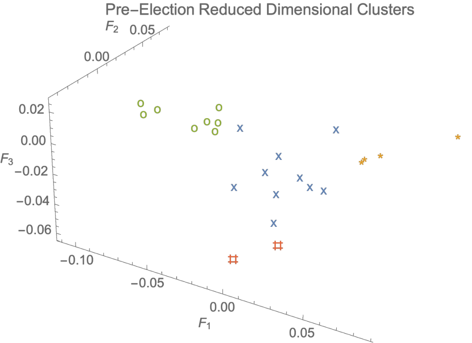
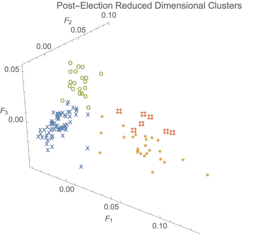
The resulting clusters each have specific spectral properties that define them. These are shown in Fig. 13, where we use box-and-whisker plots to show the ranges of each frequency bin over all elements of the cluster. Cluster 1 is composed of users whose behavior is not modeled by Eq. 7, except to say that their per-day tweet volume is composed of noise; i.e., there is no dominant frequency in their spectra. Cluster 2 is composed of users like TEN_GOP whose behavior is harmonic with period (approximately) 4 days. This cluster could be sub-divided in the post-election period since we can see a substantial amount of variation in the lower-frequency amplitudes. The 4 day periodicity is clearer in the pre-election period. Clusters 3 and 4 both have extremely sharp defining principal frequencies between bins 30 and 35 (corresponding to a 7 day periodicity). Cluster 3 has a second frequency spike between bin 60 and 65, implying a periodicity of 4 days like Cluster 2. Cluster 4 has a second frequency spike between bins 100 and 105, corresponding to a faster 2-3 day cycle, which is difficult to explain from a practical perspective. These results support Eq. 7 as modeling the tweet rate of the users in this data set and also support the idea that these accounts are controlled Twitter bots Meves and Allgemein 2016; Cable and Hugh 2019; Kellner et al. 2019.
The user names in the themselves have interesting semantic properties. In both the pre-election period and the post-election period, Cluster 3 consists of user names that appear to be regionally selected news sources. For example, OnlineMemphis, KansasDailyNews and ChicagoDailyNew are all in Cluster 3. However, there are some interesting anomalies to this rule. DetroitDailyNew and DailySanJose both appear in Cluster 1 in the post-election time period. This can be explained by anomalies in their spectra. (See Fig. 12.)
While both users have a spike between bins 30 and 35, DetroitDailyNew has a second frequency spike between bin 60 and 65 like TEN_GOP, while DailySanJose has some low frequency noise and a frequency spike between bins 100 and 105, consistent with Cluster 4. The confusion results in these two users being placed in Cluster 1.
We analyze the strategic behavior present in the clusters in Fig. 13. The three strategies are shown along with the sample points and a smoothed density histogram of the strategies. The weighted mean point of the strategies is shown as an open circle (in red). Consistent with the results illustrated in Fig. 6, there is a transition from the originate strategy to the amplify strategy for users in Cluster 1, 2 and 4. We note, however, that Cluster 3, which contains users with news-related names, continues to follow the originate strategy both before and after the US presidential election. It is also interesting to note that Cluster 2 (which contains TEN_GOP) maintains a balance between the originate and amplify strategies in contrast to users in Clusters 1 and 4.
V Topical Extraction Behavior Correlation
In this section, we construct a second set of clusters during the pre- and post-election periods based on the topics mentioned in posted tweets. We investigate the word-space dynamical system over two long time periods, and then compare the resulting clusters of behaviors (and extracted topics) with the clusters derived in the previous sections. We show evidence to support the hypothesis that the better-modeled a cluster is by Eq. 7, the fewer topical-user clusters are represented, that is, the greater the topical cohesion observed.
V.1 Algorithm for User Clustering by Text
We discuss the algorithm (Algorithm 1) used to generate clusters of users by their topical signatures. Algorithm 1 is a compilation of several pre-existing methods in natural language processing Manning and Schütze 1999 and manifold learning Tenenbaum et al. 2000; Belkin and Niyogi 2002 with a novel variant that makes use of graph analytics developed in the physics community Newman 2006; Newman 2016; Newman 2013. For this reason, we present the algorithm in detail.
We assume some minimal knowledge from statistical language processing. In particular, a stopword is a word with little value to text meaning; examples in English include “the” and “a”. Word stemming removes common endings to ground the text into a more systematic vocabulary. For example, “ending” is replaced with “end”.
We assume the input is a sequence of tweets and users. In Line 1, the tweets from User are concatenated to form a synthetic document. For the remainder of this algorithm, if is a word, let be the number of times User uses word . In Line 2, the words in the document are passed through a stemmer. Since we did not know that multiple languages were in use a priori, we used the standard English (Porter) stemmer available in Mathematica 11.3. However, multiple stemmers and language detectors could be used at this step. In Line 3, we use a custom stopword list consisting of the (stems of) most common words in a language. Again, this was specialized to English, however it is possible to generalize this step. The remaining non-stopwords were used to create term count vectors for each user in Line 4. In Line 5, a binary term-user matrix is constructed. The entries are indicators determining whether a term is used by a user. A dynamic stopword set is initialized in Step 7. In Lines 8 - 10, we iterate through the term-user matrix and determine whether a term is used by more than of the users, with . For our study we set . The rows corresponding to the words that were used by more than are added to .
Input: Raw tweets with users
Result: Clusters of Users
After deleting the dynamic stopwords, we identify keywords across all documents in Lines 13 - 18 using frequency. While it is the case that many documents follow the Zipf-Mandelbrot law and their word counts follow a Zipf-Mandelbrot distribution Zipf 1932; Mandelbrot 1965, we have found it useful to smooth these distributions and use a percentile cutoff. To do this, we fit a Gamma distribution to the word counts and then remove words that do not fall in the percentile of the distribution. For this study, we set . We chose the Gamma distribution because it has non-negative support, and being a two parameter distribution is widely adaptable. We note, there are alternate way of identifying keywords Manning and Schütze 1999.
After removing non-keywords, the term and user set is fixed and a new term-user matrix can be computed where each column is the (reduced term) term counts for the corresponding user. In Line 26, we then replace each column of , denoted with its unit vector form. That is, column of becomes .
To understand the remainder of the algorithm, we think of as a sub-matrix of the weighted adjacency matrix of a bipartite graph between terms and documents where:
Suppose that has the same structure as , but with all positive values replaced by . It is a classic result in graph theory that has in its position the number of walks of length from vertex to vertex . Thus, if is again the binarized form of , then:
Here is a square matrix whose position is the number of terms shared between User and User when . By normalizing the columns of in Line 26, we ensure that the element of is just the cosine similarity measure of the term vectors used by User and User (when ).
In Lines 27-29, we create the adjacency matrix by using the process described above and zero the diagonal. We then compute bounds (define neighbors) for each user, by finding the largest value. This is the graph theoretic equivalent of using -nearest neighbors Hart et al. 2000. In our work we set . In Lines 30 - 36, we zero an edge weight (i.e., delete edges) at index if it is less than the bound computed for user or user . In essence, this creates a version of a preferential attachment graph where (i) preference is based on shared topics, (ii) each user prefers to attach to other users but (iii) user may attach to more than users if there are more than other users who have ranked user as one of their top connections. If modeled as a directed graph, this would be an directed Barabasi-Albert network Albert and Barabási 2000 with a hidden preference based on topic.
Finally, in Lines 37 - 38, we form the graph and use maximum modularity clustering defined by Newman Newman 2006 to build user communities. This is a variation on the Isomap Tenenbaum et al. 2000 and Multidimensional Scaling Borg and Groenen 1997 approaches to manifold learning.
V.2 User-Topic Clustering Results
Applying Algorithm 1 yields 5 language-based user clusters in the pre-election period and 7 language-based clusters in the post-election period. The resulting user graphs generated in Line 37 of Algorithm 1 are shown in Fig. 14 along with the resulting maximum modularity clusters Newman 2006 generated in Line 38. The user clusters are listed in Appendix C.
We can generate word clouds from the user clusters by merging the stemmed, non-stop words used by the individuals in these clusters. This provides general information about the topical information that caused the users to be clustered. For the word clouds shown in Fig. 14, we do not remove common words.
Topics emergent in the pre-election time period are largely consistent with what is already known about this twitter data set Mueller 2019; Cable and Hugh 2019; Im et al. 2019; Lim et al. 2019. There are two groups whose comments may be designed to stoke racial tension (Word Clouds 1 and 4), one group that focuses on news (Word Cloud 5), one group devoted to politics (Word Cloud 3) and in particular Donald Trump, and a final group that seems to re-tweet information from a variety of twitter handles (Word Cloud 2).


Topics in the post-election time period are similar, but with some apparent changes in composition. In particular, one cluster (Word Cloud 1) seems to be the result of posts about the holiday(s) that occurred during the post-election period. There is a user group that focuses on news (Word Cloud 3). Interestingly, this group contains the majority of the news-themed user names (e.g., KansasDailyNews). There are at least two groups that post on race relations (Word Clouds 6 and 7). The remaining groups seem to focus on music (Word Cloud 2) and general topics related to Donald Trump (Word Clouds 5 and 6) with various subtle language differences separating these groups. As is to be expected based on the Mueller report, TEN_GOP is a member of post election user group 5 and pre-election user group 3.
V.3 Comparison with Previous Clusters
We compare the spectrum-based cluster in the pre- and post-election time periods with the topic-based clusters. This is shown in Fig. 15.
We noted in Section IV that clusters 3 and 4 in both the pre- and post-election periods had the clearest defining spectral characteristics. It is not surprising, therefore, that these groups of users show the least topical diversity. Members of pre-election (spectral) cluster 3 can be found only in pre-election user-topic cluster 5 (the news cluster), while members of pre-election (spectral) cluster 4 can be found only in pre-election user-topic cluster 2. In a similar pattern, members of post-election (spectral) cluster 3 are members of post-election user-topic cluster 3 (a news cluster). Members of post-election (spectral) cluster 4 are members of post-election user-topic clusters 1 (holiday) and 4 (Trump-related). Other spectral clusters have users that are more spread out, corresponding to less well-defined spectral properties. It is possible to create sub-clusterings of the users corresponding to both their topics and their spectra. This helps to decrease noise in the spectral clusters. We illustrate this using post-election spectral cluster 2 and post-election user-topic cluster 4. The smaller cluster contains only the users hashed_26, Jenn_Abrams, Pamela_Moore13, TEN_GOP,TheFoundingSon, and todayinsyria, but has a clear dominating frequency corresponding to a 4 day period. This is shown in Fig. 16.
Exhaustive sub-clustering using both frequency and user-topic information is left for future work.
VI Conclusion
In this paper, we have analyzed the IRA data provided by Twitter Inc. from a dynamical systems perspective. We proposed a mathematical model to describe the per-day tweet output of a subset of the users and showed that this model could be validated using spectral analysis. This analysis allowed us to cluster user behavior in a way that was distinct from prior language-based work. We also developed a novel strategy assignment that allowed us to label each tweet as being original to the IRA, amplifying of external information or spreading existing IRA information. We showed that a subset of the spectral clusters had interpretable strategic behaviors. We also showed the existence of a substantial behavioral shift within the English data set from originating information to amplifying external information just after the 2016 US presidential election. Finally, we compared the spectrally-derived user clusters to clusters derived from topics discussed and showed that more cohesive spectral clusters (based on the distinctiveness of frequency peaks) also have greater topical cohesion. We used this observation to illustrate the utility of sub-clustering using both dynamic behavior and linguistic features.
In future work, we may investigate joint clustering based on dynamic behavior and linguistic features. Additionally, it would be very instructive to conduct a very large scale analysis on general Twitter data to determine whether there are hidden attractors or fractal properties within the per-day (or per-week) time series. While this data set seems large (9M+ tweets), in reality many of the users exhibited bursty behavior making it practically impossible to reconstruct an attracting set. In the case of this data set, the presence of dominant frequencies strongly suggests that chaotic behavior is not present. However, this fact may be an important feature in differentiating bots from humans, who might exhibit far more organic (and therefore complex) tweeting patterns. In any future investigation with even more data the application of more sophisticated analytical methods using wavelet analysis or (at a minimum) spectrograms might be more instructive in understanding bursty data.
Acknowledgement
Portions of CG’s work were supported by the National Science Foundation under grant IIS-1909255. SR gratefully acknowledges support from the Center for Security Research and Education at The Pennsylvania State University.
Appendix A Alternative Spectrum and Fit Example
In this appendix, we provide an alternate spectrum and fit example from a KansasDailyNews (see Figure 17). This user has a 7 day period and is substantially less noisy that many other users.
Appendix B Spectrum Clustered User IDs for each Time Period
The following user names are associated to the two periods of investigation. We have clustered them according to their primary frequencies of posting.
Period 1 (March 8, 2016 - November 8, 2016):
Cluster 1:
TrayneshaCole, BleepThePolice, WarfareWW, Jenn_Abrams, Blk_Voice, blackmattersus, BlackToLive, hashed_68, todayinsyria, TheFoundingSon
Cluster 2:
USA_Gunslinger, TEN_GOP, gloed_up, Crystal1Johnson,
Cluster 3:
DailySanJose, hashed_37, NewspeakDaily, RoomOfRumor, hashed_57, OaklandOnline, ScreamyMonkey, KansasDailyNews,
Cluster 4:
DanaGeezus, GiselleEvns
Period 2 (November 29, 2016 - July 31, 2017)
Cluster 1:
hashed_19, hashed_39, DetroitDailyNew, DailySanJose, hashed_55, hashed_54, hashed_12, hashed_44, hashed_1, hashed_32, hashed_16, hashed_18, hashed_36, hashed_63, hashed_4, hashed_33, hashed_28, hashed_46, hashed_77, hashed_35, hashed_41, hashed_5, hashed_78, hashed_25, hashed_38, hashed_2, hashed_61, hashed_60, hashed_21, hashed_51, hashed_66, hashed_17, hashed_34, hashed_56, hashed_62, hashed_40, hashed_24, hashed_9, hashed_47, hashed_45, hashed_14, hashed_74, hashed_73, hashed_3, hashed_58, hashed_13, hashed_31, hashed_71, hashed_67, hashed_53, hashed_42, hashed_76, hashed_64, hashed_48, hashed_27, hashed_59, hashed_8, hashed_15, hashed_43, hashed_10, hashed_50, hashed_7, hashed_75, hashed_65, hashed_69
Cluster 2:
TrayneshaCole, BleepThePolice, hashed_11, hashed_52, TEN_GOP, Jenn_Abrams, hashed_29, ElPasoTopNews, hashed_49, gloed_up, blackmattersus, Crystal1Johnson, BlackToLive, Pamela_Moore13, hashed_30, hashed_26, todayinsyria, BlackNewsOutlet, TheFoundingSon, hashed_72
Cluster 3:
hashed_20, Seattle_Post, DallasTopNews, DailyLosAngeles, PhiladelphiaON, NewOrleansON, TodayNYCity, TodayCincinnati, TodayMiami, PhoenixDailyNew, ChicagoDailyNew, OnlineCleveland, Baltimore0nline, Atlanta_Online, TodayBostonMA, TodayPittsburgh, DailySanFran, Politweecs, DailySanDiego, WashingtOnline, OnlineMemphis, HoustonTopNews, StLouisOnline, KansasDailyNews, SanAntoTopNews
Cluster 4:
hashed_70, DanaGeezus, GiselleEvns, ChrixMorgan, hashed_22, hashed_23, hashed_6
Appendix C Topic Clustered Users for each Time Period
Here user names are clustered according to the topic about which they tweet during the two time periods.
Period 1 (March 8, 2016 - November 8, 2016):
Cluster 1
Blk_Voice, Crystal1Johnson, blackmattersus
Cluster 2
DanaGeezus, GiselleEvns
Cluster 3
Jenn_Abrams, TEN_GOP, TheFoundingSon, USA_Gunslinger
Cluster 4
BlackToLive, BleepThePolice, TrayneshaCole, gloed_up
Cluster 5
DailySanJose, hashed_37, KansasDailyNews, hashed_57, NewspeakDaily, OaklandOnline, hashed_68, RoomOfRumor, ScreamyMonkey, WarfareWW, todayinsyria
Period 2 (November 29, 2016 - July 31, 2017)
Cluster 1
ChrixMorgan, DanaGeezus, GiselleEvns
Cluster 2
hashed_5, hashed_9, hashed_7, hashed_8, hashed_10, hashed_18, hashed_21, hashed_25, hashed_27, hashed_33, hashed_35, hashed_39, hashed_41, hashed_43, hashed_45, hashed_51, hashed_56, hashed_62, hashed_69, hashed_71, hashed_76, hashed_78, hashed_1, hashed_53, hashed_55
Cluster 3
Atlanta_Online, Baltimore0nline, BlackNewsOutlet, BleepThePolice, ChicagoDailyNew, Crystal1Johnson, DailyLosAngeles, hashed_20, DailySanDiego, DailySanFran, DailySanJose, DallasTopNews, DetroitDailyNew, ElPasoTopNews, HoustonTopNews, KansasDailyNews, NewOrleansON, OnlineCleveland, OnlineMemphis, PhiladelphiaON, PhoenixDailyNew, Politweecs, SanAntoTopNews, Seattle_Post, hashed_72, StLouisOnline, TodayBostonMA, TodayCincinnati, TodayMiami, TodayNYCity, TodayPittsburgh, TrayneshaCole, WashingtOnline, blackmattersus, gloed_up
Cluster 4
hashed_4, hashed_6, hashed_16, hashed_17, hashed_19, hashed_23, hashed_24, hashed_26, hashed_36, hashed_38, hashed_44, Jenn_Abrams, hashed_47, hashed_50, Pamela_Moore13, hashed_60, hashed_63, hashed_70, TEN_GOP, TheFoundingSon, hashed_75, hashed_22, hashed_28, hashed_32, todayinsyria
Cluster 5
hashed_2, hashed_46, hashed_49, hashed_52, hashed_14, hashed_29, hashed_30
Cluster 6
BlackToLive, hashed_11, hashed_42, hashed_61, hashed_64, hashed_12, hashed_54
Cluster 7
hashed_3, hashed_13, hashed_15, hashed_31, hashed_40, hashed_58, hashed_59, hashed_65, hashed_67, hashed_73, hashed_77, hashed_34, hashed_48, hashed_66, hashed_74
Appendix D Hashed Usernames
hashed_1
71db45e4783602194ced17d50c4070036dfc754e9557fe918b39e58e8bf7d65b
hashed_2
1cd9dcae39203ce9df705a6ff0cb4b1961effb11c9959e48055606a108fedd44
hashed_3
f0a624171ca1c8d3177521f1362bf9eb78f1015ec3085a1eefdfa3ff9dbf73cb
hashed_4
cfb0d237487ebe3520cb83bd82df903c9c7afd5a60acba8a3576bc3ca9346467
hashed_5
efbb959a308f1bd1199a15221511bdd9e8945a3a02da83ce9d6585224733a8f6
hashed_6
8da5d23207d302647d84c4f38e4c9c48b199d9aa1cb0549940629a68b50b16cf
hashed_7
70007b94f796e3b39c18da7711327730b9e58032323c6e7b8438fc9c6acf835c
hashed_8
d225180304e4fafe5af936306b254e2cf5f2a950d6947f94c6ab44f7d51e2606
hashed_9
e35cc49080427faaf1f73e41752c5fea35a96f6c243863cd60b019661950c27e
hashed_10
8e58ab0f46d273103d9e71aa92cdaffb6e330ec7d15ae5fa79c825e2d6f291bf
hashed_11
d3f6e58202566043d909d57584be4811916859c8a09ebbe3b5239f72596d9acf
hashed_12
c465bceee4e65cc392661fafdecabc98450eb1f0b67e66a5a0d69be631f34ca5
hashed_13
14882528f53ed4b8fbadce206679b89258e363212b5a63f31777f4e93e1a5ccf
hashed_14
ef983249ef6ed5de427c4dc19ad6d966c6cf572c2505e44142e7e7261f917ae6
hashed_15
3da8a7609e8e8bbc93fb2051c4d6568ad5436d629d003735f217ecd3acd1bb7e
hashed_16
0994abf9fb8fe1bf699d0e101e9603b30f369e94a0eec1109e2f654b1a9c5caf
hashed_17
80f92e973543912617d5c7ec3bc42bd455b6970b7a52416f398ce923389d3a85
hashed_18
3f22ec97e6f7c68c28e59390710135dbfd067aa024eeb34f13dbb905b4dde4a5
hashed_19
a95a911dd6ae864c48ed062cdbe75e5c28dbe0cf57c6db3fa9dd53b654ee9845
hashed_20
8a73099860c2a4790ae6899381c0c327462e626c02ce0d3c899ce6058135786a
hashed_21
88669ad69e40d7c199af91e8107f1e0e7988d377d2e41fff77182bf42f31a1ed
hashed_22
99299a75c967aa491b27d86a60c2ffe0a6156d1b0dcb4487917f48e7e1c7ef78
hashed_23
2aae433624dcea729731ff8e44b0bdedc56e7cc9eea9bedd14bb264b07eedd5c
hashed_24
815561925624b72a95321d039bf8bdf0da5620f8475e62ce2dee37beb71abcab
hashed_25
40bd0ff013b85c7646ca07ad238bc4dc865ce2cc87034af6e7884e69481f6422
hashed_26
dce04b9807276c27a04ad521e37f061bcdfc8bc46cc6dc3d47128b263bd61124
hashed_27
a4df865b62425d5eb91b169b0bbb873434078a44b193174962a65408ed66d793
hashed_28
5ad1a4ad9a7d67c045ab752c7a946a9d847d5d7e03684174835269a193c2820e
hashed_29
f656411ab6d63685f868421c4b381779ce97b3470f701edf9ca9ebb5a0226e3d
hashed_30
21c35c77715644e10675df5bb88f02d40412785ace111edda73b40553db68bed
hashed_31
0dea399346f2f1a94e11fbc84897a35f1ccd3fcde6ea5f0e207ba0b296412e47
hashed_32
396b0b6914e425ca53c49b7f1d6cfe9757eb7368c04c657a09d83b19a8f1251e
hashed_33
beb24c4d724cb8a986f15f48e11895e7e3484598a54af5a0fef356ceb3641193
hashed_34
be762d9f6e6423c2b11320bd7b4d6abad8aed0f8a8a54f86350d0a584117eb25
hashed_35
e1c4cd815926b92691660738cd682335520a24fb08765655c261b07ef591b653
hashed_36
5788d958456ab731e042dfff6d344829c158409c1c0911d79a5de12b0a72ced1
hashed_37
fea5e166786f00c893ee247a87ab6047e3ed8727dbe4b5a67b64484dc777b070
hashed_38
ec2109adb67d2a24091026d5d9aab64dadca1fdb2f7355473c9a82f988a9c2a0
hashed_39
6791992ed85cd2e739f57d9e4f1a4d1ac119577cdece986e1e049ade25c2d793
hashed_40
8a3c0cdcac971eaf9f7802a5688faea3aadd850e5d2e214941c2ccbdcaf4ac32
hashed_41
5f452585194266b94e60c99e1dd07f808ceb2b26b10cfb939c2e5ad47888be1c
hashed_42
3c46bd68165bb49be66c657de7f09b1cbd130e65934abd29f5aec28e2a86d43d
hashed_43
e579b30026998948100e534d656b6f27770e519fab233bccaf8b6c18b4a862c8
hashed_44
0e45d2af1bbca512ab1d8fa1c2216c038f9627bb773ab4cbe351404ee7a2c93e
hashed_45
e8e7c2bfdb7272a4a7db5dfcbb01627222d934054e99469baba6a2fe5edb9f92
hashed_46
afe3c426e91f3f0e507f9cf7beceeddb2537f56e4fd3b2aab12f87fc6eee3edd
hashed_47
aa80df35407d74929dc17b058bdc679ae7f995c237f1cfd09915d970d72f72c1
hashed_48
3434652527f405b7fd0a49064a0760dc11c1eaf80a42b7c8afc800d6a3612ce2
hashed_49
6183ad40df50200d0001e2b2e0acfcdb1d5f71ddee9495874a3b1fa2b00b6e25
hashed_50
93a00b4e2d4198865a35726aab0d5c1a4205301471411a85054b714b3b89c4a9
hashed_51
fb6f6cc1a31b47965d9894b89d576add7a679a77e9022aad33d6c0c2310cd789
hashed_52
6ca21c26de8159386b71428b8bdadf732bd854614dadea9086770b71bbe1df6a
hashed_53
77755623608ac46aacd68d114868ffebad0b2cbd4d29f0fe99143d93d51864ad
hashed_54
0a0af8893cdc8454338447004eeaf65ee2934977c71ec48d3bb17e6723e1daef
hashed_55
cfe9315d7429aedb7f843a165185d91f0ae819e54026d8a22a4f6e539f5e9132
hashed_56
274d180d1de8828a8e3e7f62eec224ba9e3d04481e5d9eb29bf1cab882004a1b
hashed_57
080da9e6b0c293d8e7abe6115605790ec8bc9a5c75a2b3e60539e67e3f100875
hashed_58
f78a269be68e66b4a8c9bb5adbe49f617b6b3845134de4b9d8afe7a350bfb2cd
hashed_59
1b9adccac803d2fc7633cef02e9e6c3d64b0af50c7550a1f3d2b84c54e765cbd
hashed_60
63df8aabe784aebc5674b36a34c14dae77bfaa89e1d9bafa5a485ed32f6e2834
hashed_61
cd0e6a3af6160a511a2cea1bda54113ea9ba8ba27b70575e4d3612c6074c342b
hashed_62
11b2a99966def750bb3e9a4b52d46826cec464aefefecfb792c3b0da7e2d2be7
hashed_63
f8d82815f7d03fec70e6e8f50f859b84714024b1024979f418110feb8db9d798
hashed_64
c567f55d5430039ab5b53980a337cd6e3399e842f186e3930a92d7f2e11d27d6
hashed_65
2d60b8bc4ff97649d507084f47f8e916263eac2d7e60ab7576d7c0722c39f88b
hashed_66
366e32f7e0e3b8eac2fff4f7049e1ebd0bdc4ddfdf0c4334edac18eda8b846e6
hashed_67
96d4f0c1f4b4ed7638342a48c66c401263da4b151fdffcb98d7b775c996c3fb6
hashed_68
9ebdcf10ebedc9abf33a34e07792e18230ecd26cea77ab0f3fcdfac11fe2116f
hashed_69
eafd6b68b8855efe312fbb60d5fde0edb8632e9c0364f5044d999b0ee58837a8
hashed_70
a396435b41bb21c018281c802df9fa8d1a1eaa9b5b139c72bc1114ca62871b9c
hashed_71
21ede93ad40450cf820f249bde68d4622b61894a6597de8c6290f034acc8f059
hashed_72
aba127107267464101355d3465e86aafe41aaa31395bf82b3eb2fb801efac56f
hashed_73
8773aaa8badf887f0702db4c5c8fe1e45ff82e35ce867539fd26e9dbf804b27f
hashed_74
190df5183c66fcdf2efe5a11eb35cc827a5f0726f4788b3ee5d3aadaeeb28dbf
hashed_75
74c5eb30de3d6691e150879ee8528463c70b0feaefed9766fcbbcc8b2458221a
hashed_76
83216c1bdaf0245f9ac5b98a8c4b3cf2a1634b74d8b38dce5641f292a56c10d6
hashed_77
85fdb02196bb8c19d03a262e72132e5c8ec70bde25eaea167f012f0bc1becbf8
hashed_78
c7b1bacb73f0f3025dc09452d99b1abb22a5ce7aa0a649330f3820de07f2ecde
References
- Silva (2017) D. Silva, “Twitter releases massive data trove on russian, iranian foreign influence campaigns,” https://www.nbcnews.com/tech/social-media/twitter-releases-massive-data-trove-russian/-/iranian-foreign-influence-campaigns-n921146 (2017).
- TwitterInc. (2017) TwitterInc., “Information operations,” https://about.twitter.com/en_us/values/elections-integrity.html (2017).
- Mak (2018) T. Mak, “Russia’s Divisive Twitter Campaign Took A Rare Consistent Stance: Pro-Gun,” https://www.npr.org/2018/09/21/648803459/russias-2016-twitter-campaign-was-strongly-pro/-/gun-with-echoes-of-the-nra (2018).
- Griffin and Bickel (2018) C. Griffin and B. Bickel, “Unsupervised machine learning of open source russian twitter data reveals global scope and operational characteristics,” (2018), arXiv:1810.01466 [cs.SI] .
- Review (2018) M. T. Review, “Data mining has revealed previously unknown russian twitter troll campaigns,” https://www.technologyreview.com/s/612252/data-mining-has-revealed-previously-unknown/-/russian-twitter-troll-campaigns/ (2018).
- Popken (2018) B. Popken, NBC News https://www.nbcnews.com/tech/social-media/now-available-more-200-000-deleted-russian-troll/-/tweets-n844731 (2018).
- Kellner et al. (2019) A. Kellner, L. Rangosch, C. Wressnegger, and K. Rieck, “Political elections under (social) fire? analysis and detection of propaganda on twitter,” (2019), arXiv:1912.04143 [cs.CR] .
- Im et al. (2019) J. Im, E. Chandrasekharan, J. Sargent, P. Lighthammer, T. Denby, A. Bhargava, L. Hemphill, D. Jurgens, and E. Gilbert, “Still out there: Modeling and identifying russian troll accounts on twitter,” (2019), arXiv:1901.11162 .
- Cable and Hugh (2019) J. Cable and G. Hugh, Bots in the Net: Applying Machine Learningto Identify Social Media Trolls, Tech. Rep. (Stanford University, 2019).
- Lim et al. (2019) J. Lim, Z. Liu, and L. Zhou, in 2019 IEEE International Conference on Intelligence and Security Informatics (ISI) (2019) pp. 203–205.
- Mueller (2019) R. S. Mueller, Report On The Investigation Into Russian Interference In The 2016 Presidential Election, Tech. Rep. (Special Counsel’s Office, United States Department of Justice, 2019).
- Chen et al. (2017) Z. Chen, R. S. Tanash, R. Stoll, and D. Subramanian, in International Conference on Social Informatics (Springer, 2017) pp. 501–510.
- Beskow and Carley (2018) D. M. Beskow and K. M. Carley, in SBP-BRiMS: International Conference on Social Computing, Behavioral-Cultural Modeling and Prediction and Behavior Representation in Modeling and Simulation (2018).
- Chavoshi et al. (2016) N. Chavoshi, H. Hamooni, and A. Mueen, in 2016 IEEE 16th International Conference on Data Mining (ICDM) (2016) pp. 817–822.
- Radziwill and Benton (2016) N. M. Radziwill and M. C. Benton, ArXiv abs/1605.06555 (2016).
- Khan and Thakur (2018) Y. Khan and S. Thakur, in 2018 International Conference on Intelligent and Innovative Computing Applications (ICONIC) (2018) pp. 1–5.
- Ozbay and Alatas (2020) F. A. Ozbay and B. Alatas, Physica A: Statistical Mechanics and its Applications 540, 123174 (2020).
- Watson (2015) M. C. Watson, in 2015 IEEE International Conference on Big Data (Big Data) (2015) pp. 793–800.
- Gao et al. (2016) J. Gao, H. Shen, S. Liu, and X. Cheng, in Proceedings of the 25th International Conference Companion on World Wide Web, WWW ’16 Companion (International World Wide Web Conferences Steering Committee, Republic and Canton of Geneva, CHE, 2016) pp. 33–34.
- Stillgherrian (2020) Stillgherrian, “Twitter bots and trolls promote conspiracy theories about Australian bushfires,” https://www.zdnet.com/article/twitter-bots-and-trolls-promote-conspiracy/-/theories-about-australian-bushfires/ (2020).
- Manning and Schütze (1999) C. D. Manning and H. Schütze, Foundations of Statistical Natural Language Processing (MIT Press, 1999).
- Inc. (2019) T. Inc., “Getting Started: Twitter Help Center,” https://help.twitter.com/en/twitter-guide (2019).
- Griffin and Belmonte (2017) C. Griffin and A. Belmonte, Physical Review E 95, 052309 (2017).
- Badawy et al. (2018) A. Badawy, E. Ferrara, and K. Lerman, CoRR abs/1802.04291 (2018), arXiv:1802.04291 .
- Cleary (2019) G. Cleary, “Twitterbots: Anatomy of a Propaganda Campaign,” https://www.symantec.com/blogs/threat-intelligence/twitterbots-propaganda-disinformation (2019).
- Lab (2018) A. C. D. F. R. Lab, “TrollTracker: Twitter Troll Farm Archives,” https://medium.com/dfrlab/trolltracker-twitter-troll-farm-archives/-/8d5dd61c486b (2018).
- Thompson (2018) A. Thompson, “This is How We Troll,” https://www.ceros.com/originals/russian-tweet-bot-data/ (2018).
- Di Lorenzo (2013) R. Di Lorenzo, in Basic Technical Analysis of Financial Markets (Springer, 2013) pp. 189–220.
- Friedlander et al. (2003) D. Friedlander, C. Griffin, N. Jacobson, S. Phoha, and R. R. Brooks, EURASIP J. Applied Signal Processing 4, 371 (2003).
- Jolliffe (2011) I. Jolliffe, Principal component analysis (Springer, 2011).
- Kaufman et al. (1987) L. Kaufman, P. Rousseeuw, and Y. Dodge, “Clustering by means of medoids in statistical data analysis based on the,” (1987).
- Meves and Allgemein (2016) N. Meves and K. Allgemein, “Der Bot Boost #merkelmussbleiben,” https://www.wahl.de/aktuell/2016/08/05/social-bot-bundesregierung/ (2016).
- Tenenbaum et al. (2000) J. B. Tenenbaum, V. d. Silva, and J. C. Langford, Science 290, 2319 (2000), http://science.sciencemag.org/content/290/5500/-/2319.full.pdf .
- Belkin and Niyogi (2002) M. Belkin and P. Niyogi, in Advances in neural information processing systems (2002) pp. 929–936.
- Newman (2006) M. E. J. Newman, Proceedings of the National Academy of Sciences 103, 8577 (2006), http://www.pnas.org/content/103/23/8577.full.pdf .
- Newman (2016) M. E. J. Newman, Phys. Rev. E 94, 052315 (2016).
- Newman (2013) M. E. J. Newman, Phys. Rev. E 88, 042822 (2013).
- Zipf (1932) G. K. Zipf, Selected Studies of the Principle of Relative Frequency in Language (Harvard University Press, 1932).
- Mandelbrot (1965) B. Mandelbrot, in Language (Penguin Books, 1965).
- Hart et al. (2000) P. E. Hart, D. G. Stork, and R. O. Duda, Pattern Classification (Wiley-Interscience, 2000).
- Albert and Barabási (2000) R. Albert and A.-L. Barabási, Phys. Rev. Lett. 85, 5234 (2000).
- Borg and Groenen (1997) I. Borg and P. Groenen, Modern Multidimensional Scaling: theory and applications, (Springer-Verlag, New York, NY, 1997).