Topological metric detects hidden order in disordered media
Abstract
Recent advances in microscopy techniques make it possible to study the growth, dynamics, and response of complex biophysical systems at single-cell resolution, from bacterial communities to tissues and organoids. In contrast to ordered crystals, it is less obvious how one can reliably distinguish two amorphous yet structurally different cellular materials. Here, we introduce a topological earth mover’s (TEM) distance between disordered structures that compares local graph neighborhoods of the microscopic cell-centroid networks. Leveraging structural information contained in the neighborbood motif distributions, the TEM metric allows an interpretable reconstruction of equilibrium and non-equilibrium phase spaces and embedded pathways from static system snapshots alone. Applied to cell-resolution imaging data, the framework recovers time-ordering without prior knowledge about the underlying dynamics, revealing that fly wing development solves a topological optimal transport problem. Extending our topological analysis to bacterial swarms, we find a universal neighborhood size distribution consistent with a Tracy-Widom law.
Discrete particulate objects, from atoms to cells, compose the majority of physical and living systems. Modern microscopy and simulation techniques enable us to study the elementary building blocks of solids Binnig and Rohrer 1987; Sugimoto et al. 2007, colloidal and granular materials Glotzer and Solomon 2007; Soni et al. 2019; Nauer et al. 2019, bacterial biofilms Hartmann et al. 2019; Dell’Arciprete et al. 2018, and tissues Etournay et al. 2015 with unprecedented resolution over large scales. These experimental and computational advances have highlighted the importance of local spatial organization Pearce et al. 2019a and disorder Goodrich et al. 2014 for the global behaviors of both equilibrium and non-equilibrium materials, spurring substantial theoretical efforts to link discrete microstructure with macroscale properties. Prime examples include the recent successful characterizations of epithelial cell (EC) layers and other cellular materials through the geometric Bi et al. 2016; Bi et al. 2015 and topological Lazar et al. 2012; Mason et al. 2012; Schweinhart et al. 2016; Wenzel et al. 2019 analysis of Voronoi and Delaunay tesselations Aurenhammer et al. 2013. In spite of such major progress, high-resolution data continue to pose fundamental conceptual and practical challenges regarding the proper classification of discrete physical and biological structures. Specifically, it is still unclear whether one can recover parametric embeddings, phase space dimensions and time ordering from a topological analysis of static snapshots alone, and whether such analysis can help reveal the governing principles of multicellular development.
To tackle these problems, we introduce here a topological earth mover’s (TEM) distance by combining ideas from statistical topology Lazar et al. 2012; Mason et al. 2012; Schweinhart et al. 2016; Ronellenfitsch et al. 2015; Rocks et al. 2020 and optimal transport theory Essid and Solomon 2018; Solomon et al. with non-equilibrium statistical mechanics Ronhovde et al. 2012. The TEM metric compares two discrete material structures by quantifying the statistical differences in the local network topology of their Delaunay triangulations (Fig. 1). Intuitively, computing TEM(, ) amounts to estimating the smallest number of edge-flips needed to make the local network topology of material statistically indistinguishable from the local network topology of material . Physically, this procedure can be interpreted as finding the average lowest-energy path connecting two disordered structures, and we provide an efficient algorithm for realizing this computationally demanding task for systems with particles SM.
To demonstrate the practical potential of this framework for the analysis of both equilibrium and non-equilibrium systems, we present a broad set of applications: First, we show that the TEM metric successfully distinguishes jammed disordered packings of both monodisperse and polydisperse ellipsoids. Thereafter, we use the TEM framework to reconstruct the non-equilibrium phase diagram of active Brownian particle (ABP) simulations without recourse to time resolved data. Next, by measuring the pairwise TEM distances between unsorted experimental images of a developing fruit fly wing, we are able to reconstruct their temporal ordering and discover that wing development follows an optimal transport geodesic, suggesting a previously unrecognized optimization principle in tissue development. Finally, by extending our topological analysis to single-cell resolution data from bacterial swarming experiments, we observe a universal neighborhood size distribution consistent with a Tracy-Widom law.

To define the TEM distance, we consider the specific example of a two-dimensional (2D) cell layer as shown in Fig. 1(a), although all subsequent definitions generalize to arbitrary point sets in or . Our starting point is the Delaunay triangulation Aurenhammer et al. 2013 of the cell centroid positions as shown in Fig. 1(a). In practice, it is often sufficient to take the positions of the EC nuclei as vertices of the Delaunay network van Drongelen et al. 2018. If two random realizations of such networks are generated by the same physical or biological process, they will have different vertex positions and topology, but their local statistical properties (local connectivity patterns, etc.) will be identical provided the networks are sufficiently large. This fact has been exploited previously to define entropic Mason et al. 2012 and earth mover’s distances between cell complexes Schweinhart et al. 2016. Here, we extend these ideas to define a physically motivated topological metric that measures statistical differences in the local Delaunay triangulations around vertices. Specifically, we define for each vertex a local neighborhood of radius , which consists of all the vertices that are not more than edges away from the central vertex (see red subgraph corresponding to in Fig. 1a). We found that suffices for many practical applications SM. Although can, in principle, be chosen arbitrarily large, TEM computations become expensive for a larger neighborhoods; we therefore focus on the case from now on. The local neighborhoods of two vertices are of the same topological type if they are graph-isomorphic. Counting the occurrences of the various neighborhood types across all vertices yields a probability distribution that characterizes the topo-statistical state of the cell network.
To provide an intuitive physical motivation for the TEM metric, let us recall that the Delaunay network is invariant under infinitesimal perturbations and can change only through a topological T1 transition (Fig. 1b). For EC layers there is an energy barrier to T1 transitions Bi et al. 2014, and so the energy cost to transform from one neighborhood type to another is directly related to the number of T1 transitions required. For other packed systems there typically exist similar energetic cost for changing neighbors through T1 transitions. Motivated by this, we can define the energetic distance between two neighborhoods as the minimum number of T1 transitions separating them. This mathematically well-defined metric Lawson 1972; SM induces naturally a secondary graph structure, known as the flip graph Bose and Hurtado 2009, where nodes correspond to neighborhood types and are linked with an edge if they are one T1 transition away from each other (Fig. 1c). The minimum path length between two nodes on the flip graph is the smallest number of T1 transitions needed to move between the corresponding neighborhood types. Moreover, the distribution of neighborhood types in the EC layer can now be viewed as a distribution on the nodes of the flip graph (blue box in Fig. 1d).

Armed with this intuition, we can now define the TEM distance between the Delaunay triangulations of two materials and in a natural manner as the earth mover’s or, equivalently, Wasserstein distance Essid and Solomon 2018 between their neighborhood distributions and over the flip graph: If is the probability of neighborhood occuring in material , and is the probability of neighborhood occuring in material , then a transport map, , from to satisfies , , see Fig. 1(d). Then, the TEM distance between and is
| (1) |
where is the distance between the neighborhoods and on the flip graph, and the minimum is taken over all possible transport maps . We emphasize that, in contrast to widely used entropic distances measures between distributions Mason et al. 2012, the definition of TEM uses the physically relevant information encoded in the metric structure of the underlying observable space, which in our case reflects the typical energy cost of a T1 transitions between network motifs. As a consequence, TEM generally outperforms purely entropic Kullback-Leibler/Jensen-Shannon divergences when one needs to distinguish complex structures that are characterized by weakly overlapping distributions; see Ref. Solomon and the Supplemental Material SM for explicit examples.
For large systems, the minimization problem (1) becomes computationally challenging. We combined two algorithmic insights SM to calculate TEM efficiently for disordered materials with millions of particles. Building on a modification of the Weinberg algorithm Weinberg 1966, our numerical scheme SM first determines the flip-graph distances of observed neighborhood motifs in steps. Given , the minimization over the transport maps can be recast as an minimum cost flow problem SM; Essid and Solomon 2018, which is efficiently solved with linear programming Dunning et al. 2017. To demonstrate the broad applicability of our TEM framework, we focus in the remainder on applications relevant to current major research areas: colloidal packings, collective far-from-equilibrium dynamics, tissue development, and spatio-temporally heterogeneous multicellular systems.


Recent advances in the fabrication of geometrically complex colloids Glotzer and Solomon 2007; Soni et al. 2019 and confocal imaging techniques Hartmann et al. 2019 have led to a renewed practical and theoretical interest in the characterization of granular Donev et al. 2004; Nauer et al. 2019 and biological materials Hartmann et al. 2019; Dell’Arciprete et al. 2018. Of particular importance in this context are the often fundamentally different behaviors of monodisperse Torquato and Stillinger 2010 and polydisperse Aranson and Tsimring 2006 colloidal systems. While the former are much better understood theoretically, the latter are often practically more relevant to natural systems and processes, such as particle segregation seen in industrial agriculture, cereals, or avalanches Kudrolli 2004. To demonstrate the usefulness of the TEM framework for capturing the essential topo-statistical differences between and across mono- and polydisperse systems, we generated jammed disordered packings of 10,000 ellipsoids using an event-driven packing code Donev et al. 2005. Specifically, we were interested in distinguishing two different pathways for transitioning from a monodisperse packing of spheres (ellipsoids with aspect ratio 1:1) to a monodisperse packing of ellipsoids with aspect ratio 1:3 (Fig. 2a). The first ‘monodisperse’ transition path was realized by simulating 12 monodisperse packings of ellipsoids with aspect ratios varying from 1:1 to 1:3 (bottom path in Fig. 2a). The second ‘polydisperse’ transition path was realized by simulating 12 different binary mixtures of 1:1 and 1:3 ellipsoids (top path in Fig. 2a). Computing the TEM distances between all pairs of simulations produces the symmetric TEM distance matrix shown in Fig. 2(b). Given this matrix, it is natural to seek a faithful low-dimensional embedding in Euclidean space that approximately preserves the TEM distance structure. To construct the embedding we choose Multi-Dimensional Scaling (MDS), a generalized principal component (PC) analysis based on the TEM distance Borg and Groenen 2005. Since each pathway corresponds to a 1D manifold (as only one parameter is varied in each case), the phase space can be embedded in ; indeed the embedding clearly distinguishes the two different pathways (Fig. 2c). To find the dimensionality of the phase space, we calculate the residual variance which plateaus at the relevant dimension SM; Tenenbaum et al. 2000 and correctly identifies the ellipsoid embedding as 2D (Fig. 2d). We show in the Supplementary Information SM that the same approach can be used to infer the non-equilibrium phase space of active Brownian particle (ABP) simulations Fily et al. 2014 from instantaneous system configurations. More broadly, these examples illustrate how the TEM metric can discover phase spaces from configurational snapshots alone.
In the remainder, we show that the topological analysis of data from two recent experiments Etournay et al. 2015; Jeckel et al. 2019 can reveal previously unrecognized biophysical optimization principles and universal statistical signatures. We begin by considering shuffled images (Fig. 3a-e) of developing fruit fly embryo wings Etournay et al. 2015; Etournay et al. 2016. Using the Delaunay triangulation of the cell centroids, hierarchical clustering Ward 1963 of the TEM distance matrix of the shuffled images (Fig. 3f) reveals three developmental main phases (Fig. 3g). The resulting MDS embedding is essentially 1D, with the first principal component corresponding to time (Fig. 3h), and thus restores the temporal order of the data (Fig. 3i). This shows how the TEM framework can be used to infer temporal ordering from ensemble measurements Pearce et al. 2019b. More importantly, however, the TEM analysis reveals the developmental trajectory of the fly wing follows a topological geodesic, a continuous curve that minimizes the total length with respect to the TEM distance. Whilst earth mover’s geodesics are in general not unique, a unique path can be found by additionally minimizing transport dissipation Solomon et al.; SM. The data fluctuates closely around this minimum-dissipation geodesic (red curve in Fig. 3h), meaning that fly wing development approximately solves a dissipation-constrained topological optimal transport problem.
Finally, we provide a more detailed characterization of the neighborhood motif distributions in 2D non-equilibrium systems. To this end, we analyze recent bacterial swarming experiments Jeckel et al. 2019 using machine learning SM to identify individual cells (Fig. 4a,b). By determining the motif size distributions for snapshots taken at different space-time locations in a growing swarm, we find that both mean and variance vary systematically with space, time, and cell density (Fig. 4c-e). Strikingly, after rescaling to zero mean and unit variance, the combined motif size distribution closely matches SM a universal Tracy-Widom (TW) distribution (Fig. 4f). TW distributions were recently reported for growing fluctuating fronts Takeuchi et al. 2011, dynamics of self-assembly Makey et al. 2020, active particle dynamics Chen et al. 2018; Tracy and Widom 2009, and phase transitions between strongly and weakly coupling regimes Majumdar and Schehr 2014. We also find TW motif size distributions in the ABP and fly wing data when subsampling from the liquid-like phase SM, suggesting that TW distributions play a central role in the topo-statistics of non-equilbrium systems.
To conclude, the TEM metric framework will be broadly applicable, from single-cell RNA-sequencing Shalek et al. 2013, cryo-electron microscopy Fischer et al. 2010 and organoid characterization Dekkers et al. 2019, to structural transitions in living Bi et al. 2016; Hartmann et al. 2019 and nonliving Glotzer and Solomon 2007 matter. In particular, it enables a direct comparison of the topological statistical properties of a wide range of fundamentally different systems, the only requirement being that transitions between basic motifs (Delaunay neighborhood structures, DNA strings, etc.) can be mapped onto a joint flip-graph structure.
This work was supported by a MathWorks Fellowship (D.J.S.), a James S. McDonnell Foundation Complex Systems Scholar Award (J.D.), and the Robert E. Collins Distinguished Scholar Fund (J.D.). We thank Martin Abt for help with cell segmentation and the MIT SuperCloud and Lincoln Laboratory Supercomputing Center for providing HPC resources.
References
- Binnig and Rohrer (1987) G. Binnig and H. Rohrer, Rev. Mod. Phys. 59, 615 (1987).
- Sugimoto et al. (2007) Y. Sugimoto, P. Pou, M. Abe, P. Jelinek, R. Pérez, S. Morita, and Ó. Custance, Nature 446, 64 (2007).
- Glotzer and Solomon (2007) S. C. Glotzer and M. J. Solomon, Nature Materials 6, 557 (2007).
- Soni et al. (2019) V. Soni, E. Bililign, S. Magkiriadou, S. Sacanna, D. Bartolo, M. Shelley, and W. Irvine, Nat. Phys. 15, 1188 (2019).
- Nauer et al. (2019) S. Nauer, L. Böttcher, and M. A. Porter, J. Complex Networks , doi:10.1093/comnet/cnz037 (2019).
- Hartmann et al. (2019) R. Hartmann, P. Singh, P. Pearce, R. Mok, B. Song, F. Díaz-Pascual, J. Dunkel, and K. Drescher, Nat. Phys. 15, 251 (2019).
- Dell’Arciprete et al. (2018) D. Dell’Arciprete, M. Blow, A. Brown, F. Farrell, J. Lintuvuori, A. McVey, D. Marenduzzo, and W. Poon, Nat. Commun. 9, 4190 (2018).
- Etournay et al. (2015) R. Etournay, M. Popović, M. Merkel, A. Nandi, C. Blasse, B. Aigouy, H. Brandl, G. Myers, G. Salbreux, F. Jülicher, and S. Eaton, eLife 4, e07090 (2015).
- Pearce et al. (2019a) P. Pearce, B. Song, D. J. Skinner, R. Mok, R. Hartmann, P. K. Singh, H. Jeckel, J. S. Oishi, K. Drescher, and J. Dunkel, Phys. Rev. Lett. 123, 258101 (2019a).
- Goodrich et al. (2014) C. P. Goodrich, A. J. Liu, and S. R. Nagel, Nature Physics 10, 578 (2014).
- Bi et al. (2016) D. Bi, X. Yang, M. C. Marchetti, and M. L. Manning, Phys. Rev. X 6, 021011 (2016).
- Bi et al. (2015) D. Bi, J. H. Lopez, J. M. Schwarz, and M. L. Manning, Nature Physics 11, 1074 (2015).
- Lazar et al. (2012) E. A. Lazar, J. K. Mason, R. D. MacPherson, and D. J. Srolovitz, Phys. Rev. Lett. 109, 095505 (2012).
- Mason et al. (2012) J. K. Mason, E. A. Lazar, R. D. MacPherson, and D. J. Srolovitz, Phys. Rev. E 86, 051128 (2012).
- Schweinhart et al. (2016) B. Schweinhart, J. K. Mason, and R. D. MacPherson, Phys. Rev. E 93, 062111 (2016).
- Wenzel et al. (2019) D. Wenzel, S. Praetorius, and A. Voigt, J. Chem. Phys. 150, 164108 (2019).
- Aurenhammer et al. (2013) F. Aurenhammer, R. Klein, and D.-T. Lee, Voronoi Diagrams and Delaunay Triangulations, 1st ed. (World Scientific Publishing Co., Inc., River Edge, NJ, USA, 2013).
- Ronellenfitsch et al. (2015) H. Ronellenfitsch, J. Lasser, D. Daly, and E. Katifori, PLoS Comput. Biol. 11, e1004680 (2015).
- Rocks et al. (2020) J. W. Rocks, A. J. Liu, and E. Katifori, Phys. Rev. Research 2, 033234 (2020).
- Essid and Solomon (2018) M. Essid and J. Solomon, SIAM J. Sci. Comput. 40, A1961 (2018).
- (21) J. Solomon, R. Rustamov, L. Guibas, and A. Butscher, arXiv:1603.06927 .
- Ronhovde et al. (2012) P. Ronhovde, S. Chakrabarty, D. Hu, M. Sahu, K. K. Sahu, K. F. Kelton, N. A. Mauro, and Z. Nussinov, Scientific Reports 2, 329 (2012).
- (23) Supplementary Information.
- Etournay et al. (2016) R. Etournay, M. Merkel, M. Popović, H. Brandl, N. Dye, B. Aigouy, G. Salbreux, S. Eaton, and F. Jülicher, eLife 5, e14334 (2016).
- van Drongelen et al. (2018) R. van Drongelen, T. Vazquez-Faci, T. A. Huijben, M. van der Zee, and T. Idema, J. Theor. Biol. 454, 182 (2018).
- Bi et al. (2014) D. Bi, J. H. Lopez, J. M. Schwarz, and M. L. Manning, Soft Matter 10, 1885 (2014).
- Lawson (1972) C. L. Lawson, Discrete Math. 3, 365 (1972).
- Bose and Hurtado (2009) P. Bose and F. Hurtado, Comput. Geometry 42, 60 (2009).
- (29) J. Solomon, arXiv:1801.07745 .
- Weinberg (1966) L. Weinberg, IEEE Trans. Circuit Theory 13, 142 (1966).
- Dunning et al. (2017) I. Dunning, J. Huchette, and M. Lubin, SIAM Review 59, 295 (2017).
- Jeckel et al. (2019) H. Jeckel, E. Jelli, R. Hartmann, P. K. Singh, R. Mok, J. F. Totz, L. Vidakovic, B. Eckhardt, J. Dunkel, and K. Drescher, Proc. Nat. Acad. Sci. 116, 1489 (2019).
- Donev et al. (2004) A. Donev, I. Cisse, D. Sachs, E. A. Variano, F. H. Stillinger, R. Connelly, S. Torquato, and P. M. Chaikin, Science 303, 990 (2004).
- Torquato and Stillinger (2010) S. Torquato and F. H. Stillinger, Rev. Mod. Phys. 82, 2633 (2010).
- Aranson and Tsimring (2006) I. S. Aranson and L. S. Tsimring, Rev. Mod. Phys. 78, 641 (2006).
- Kudrolli (2004) A. Kudrolli, Rep. Prog. Phys. 67, 209 (2004).
- Donev et al. (2005) A. Donev, S. Torquato, and F. H. Stillinger, J. Comput. Phys. 202, 765 (2005).
- Borg and Groenen (2005) I. Borg and P. J. F. Groenen, “Modern multidimensional scaling: Theory and applications,” (Springer, 2005) Chap. 12, pp. 201–268, 2nd ed.
- Tenenbaum et al. (2000) J. B. Tenenbaum, V. d. Silva, and J. C. Langford, Science 290, 2319 (2000).
- Fily et al. (2014) Y. Fily, S. Henkes, and M. C. Marchetti, Soft Matter 10, 2132 (2014).
- Ward (1963) J. H. Ward, J. Am. Stat. Assoc. 58, 236 (1963).
- Pearce et al. (2019b) P. Pearce, F. G. Woodhouse, A. Forrow, A. Kelly, H. Kusumaatmaja, and J. Dunkel, Nat. Commun. 10, 5368 (2019b).
- Takeuchi et al. (2011) K. A. Takeuchi, M. Sano, T. Sasamoto, and H. Spohn, Scientific Reports 1, 34 (2011).
- Makey et al. (2020) G. Makey, S. Galioglu, R. Ghaffari, E. D. Engin, G. Yıldırım, Ö. Yavuz, O. Bektaş, Ü. S. Nizam, Ö. Akbulut, Ö. Şahin, et al., Nat. Phys. 16, 795 (2020).
- Chen et al. (2018) Z. Chen, J. de Gier, I. Hiki, and T. Sasamoto, Phys. Rev. Lett. 120, 240601 (2018).
- Tracy and Widom (2009) C. A. Tracy and H. Widom, Commun. Math. Phys. 290, 129 (2009).
- Majumdar and Schehr (2014) S. N. Majumdar and G. Schehr, J. Stat. Mech.: Theory Exp. 2014, P01012 (2014).
- Shalek et al. (2013) A. K. Shalek, R. Satija, X. Adiconis, R. S. Gertner, J. T. Gaublomme, R. Raychowdhury, S. Schwartz, N. Yosef, C. Malboeuf, D. Lu, et al., Nature 498, 236 (2013).
- Fischer et al. (2010) N. Fischer, A. L. Konevega, W. Wintermeyer, M. V. Rodnina, and H. Stark, Nature 466, 329 (2010).
- Dekkers et al. (2019) J. F. Dekkers, M. Alieva, L. M. Wellens, H. C. R. Ariese, P. R. Jamieson, A. M. Vonk, G. D. Amatngalim, H. Hu, K. C. Oost, Snippert, et al., Nature Protocols 14, 1756 (2019).
Supplemental Material:
Topological metric detects hidden order in disordered media
Dominic J. Skinner,1 Boya Song,1, Hannah Jeckel2,3, Eric Jelli2,3, Knut Drescher2,3, and Jörn Dunkel1
1Department of Mathematics, Massachusetts Institute of Technology, Cambridge, Massachusetts 02139-4307, USA
2Max Planck Institute for Terrestrial Microbiology, 35043 Marburg, Germany
3Department of Physics, Philipps-Universität Marburg, 35043 Marburg, Germany
(Dated: August 11, 2026)
.1 Voronoi diagrams and Delaunay triangulations
Given a set of points in , the Voronoi tessellation partitions into regions known as Voronoi cells. A point is in the Voronoi cell associated with if is closer to than to any other . The Delaunay triangulation is a graph with vertices at the points in , with two points sharing an edge if their corresponding Voronoi cells share a face. For more properties refer to Aurenhammer et al. 2013.
.2 Interior and exterior points
For simulations with periodic boundary conditions the Deluanay graph extends periodically and there are no boundary cases. For simulations or experiments that are not periodic, there exist exterior points on the edge which may have quite different properties from points in the bulk. We do not wish to include edge effects and so we only take local networks of radius for points at least edges away from exterior points. Exterior points are identified by calculating the alpha shape, or concave hull Edelsbrunner et al. 1983. In short, a point is an exterior point if a circle (or sphere in ) of radius can intersect that point without enclosing any other points. For every point , there is a largest circle which intersects , but does not include any other points; call its radius . For the non-periodic Drosophila example, (median ) identifies cells on the edge without incorrectly identifying interior points (Fig. S1).
.3 Storing and comparing networks
Many thousands of topologically distinct networks were observed, requiring fast methods to store and compare them. The approach taken here was to replace each network with a vector of integers that uniquely represents its topological type. Once represented as a vector, the networks can be stored as a dictionary with an cost to read for topologically distinct graphs. Calculating the probability distribution for networks is then , rather than the cost that would be required if one used an algorithm that could only compare two graphs at a time.
To encode the topology we use a modified Weinberg algorithm. The Weinberg algorithm uniquely encodes the topology of a triply connected planar graph, where triply connected means at least three vertices need to be removed to disconnect the graph Weinberg 1966; Lazar et al. 2012. The local network is triply connected, see Fig. S2.
Proof: First show the local network of radius is triply connected. Suppose two vertices are removed, if the central vertex is kept, as everything is connected to the central vertex, the graph is still connected. Suppose now that the central vertex and one other vertex are removed, as in (a). Label the remaining vertices by their anti-clockwise ordering about the central vertex for a particular embedding. Then as the local network is a triangulation, the central vertex and vertices , form a triangle, so vertex is connected to , hence the network remains connected.
Now consider a local network of arbitrary radius, and a path between two vertices, and . If no vertices on this path are removed and are still connected. If one vertex is removed, vertex 2 in (b), the path enters the vertex from 1 and leaves toward 3. But 1 and 3 are in the local network of radius 1 around vertex 2, hence are connected, and so an alternative path from to can be found.
The final case is when vertex 3 is also deleted, so an alternative path to vertex 4 must be found, as in (c). Here, note that as the network is a triangulation, vertices 2 and 3 are connected to a common vertex, vertex 5 which is in the local network of radius 1 for both. So 1 and 5 are connected as the local network of radius 1 is connected around 2, but 5 and 4 are also connected as the local network of radius 1 is connected around 3. Therefore an alternative path from to can be found, hence the network remains connected.
In short, Weinberg’s algorithm canonically labels Eulerian circuits, and from all possible Eulerian circuit picks the lexographically first labeling. This labeling is taken as the vector; every isomorphic graph has the same vector and if two graphs have the same vector they are isomorphic. The procedure for finding the Eulerian circuit from a given oriented starting edge is detailed in algorithm 1, and the canonical labeling for a particular starting edge is detailed in algorithm 2. The total algorithm is described in algorithm 3.
Weinberg’s algorithm as described in Weinberg 1966 differers from algorithm 3 in that it traverses every edge in both directions rather than just the edges originating at the central vertex and so recognizes the same graph with different embeddings as isomorphic. The local Delaunay network is a near triangulation meaning all of the faces are triangular except the one at infinity Bose and Hurtado 2009, so there is only one embedding that we will observe (together with the mirrored embedding). We also only define isomorphism between egocentric networks to mean the networks are isomorphic and they have the same central vertex (it is possible for an egocentric network to have two possible candidates for the central vertex, although these are quite rare in practice). Therefore to check if two egocentric networks are isomorphic we need only consider the labelings that start by moving away from the central vertex. If they are isomorphic they share the same labelings. The resulting vector will not be the same as the vector calculated by trying all edges, but still works as a topological identifier when compared only to other vectors calculated in the same manner.
The algorithm in Weinberg 1966 finds the Weinberg vector in time, as finding the path and labeling it (which can be done simultaneously) takes time, and this must be done for edges. By only taking the edges that start at the central vertex, which is typically , the calculation grows like as the size of the local network grows. For local networks of radius this typically allows the algorithm to run 10-20 times faster.
.4 Calculating the flip graph
Given observed networks, we wish to calculate which are connected by an edge in the flip graph, from which the minimum path length between two networks gives a measure of distance between them. This measure of distance is similar to the Levenshtein distance between two strings, although in that case distances are calculated, as needed, using dynamic programming Wagner and Lowrance 1975. Here, path lengths on the flip graph give distances, but this requires checking if up to edges exist. Instead we are able to calculate the flip graph in time using algorithm 4. The central insight is that after a T1 transition or flip, path distances to the central vertex either do not increase or do not decrease, as proved in Fig. S4. After flipping, the new graph need not be a local network, but due to the claim in Fig. S4, for one of the local networks, flipping means the other local network is a subgraph of the flipped graph (see Fig. S5). Since this requires calculating a Weinberg vector for potentially each edge of a network, the total cost is .
The flip graph is connected, but in practice this calculation often yields a disconnected graph. This occurs when the path between two states goes through states that were not observed in the observed networks (but do theoretically exist). If this occurs for a few isolated states that make up a negligible proportion of the total, then the largest connected component can be taken and these isolated states can be ignored. If the number of disconnected states is large, then the observed networks can be augmented by additional networks observed in a Poisson-Voronoi process or similar Lazar et al. 2012, and a larger flip graph can be calculated. Networks are added until the connected component of the new flip graph contains all (or almost all) of the original observed networks.
.5 Calculating the TEM distance
The topological earth mover’s (TEM) distance is defined to be the earth mover’s distance between two probability distributions on the flip graph,
| (S1a) | |||
| where the sum is taken over all pairs of networks , is the minimum path length on the flip graph between networks and , and is a map between distributions satisfying | |||
| (S1b) | |||
Rather than optimize over all possible maps , the problem can be rephrased as a minimum cost flow problem over the flip graph Essid and Solomon 2018. This is done by first converting to a minimum cost flow problem over the complete graph on vertices, where the weight, or cost, on the edge between and is , and each vertex is a source or sink with strength . This is then equivalent to solving on the flip graph, because the cost of sending mass directly from to is the same cost as sending it through the minimum length path between and .
The minimum cost flow is converted into the standard formulation, by taking two additional nodes, one a source, one a sink, and connecting every existing source to the new source by an edge with a capacity of the existing source strength and connecting every existing sink to the new sink by an edge with demand of the existing sink strength. With the exeption of the new source and sink, all other sources and sinks are then set to strength 0. To reduce the stiffness of the problem, each capacity was multiplied by and each demand was multiplied by . Under this relaxation of the problem, the algorithm always converged, and the additional error was found to be . For significantly larger or stiffer problems, approximations to optimal transport, such as entropic regularization are possible Essid and Solomon 2018, but were not required here.
.6 Residual variance

The residual variance is defined as , where is the (Euclidean) distance matrix in the embedded space, is an unembedded distance matrix, and is the linear correlation coefficient Tenenbaum et al. 2000. To calculate the residual variance, we do not take the TEM distance matrix, instead we take as the Isomap distance matrix derived from the TEM distance matrix Tenenbaum et al. 2000. In short, this means replacing the TEM distance between two points with their distance along the manifold; local distances are preserved and global distances become a sum of local distances along the path between two points Tenenbaum et al. 2000. Local here means the nearest neighbors of a point (knn), where is a parameter to be chosen. The dimension of the manifold on which the points lie is the dimension for which the residual variance becomes negligible or does not decrease for higher dimensional embeddings Tenenbaum et al. 2000.
To understand why Isomap produces the most accurate estimate of dimension, consider the example of a 2D spiral; a 1D manifold with non-trivial embedding in 2D Euclidean space (Fig. S6a). The 2D MDS embedding maintains the spiral (Fig. S6b), as does a 2D Isomap embedding with a large number of neighbors (Fig. S6c). In contrast, a 2D Isomap embedding using 2 neighbors “unrolls” the shape to get a straight line (Fig. S6d). Therefore, Isomap can correctly identify the manifold as 1D, whereas MDS incorrectly identifies the manifold as 2D (Fig. S6e). That said, the MDS embedding preserves the non-trivial structure of the manifold in 2D; for this reason we stick with MDS embeddings for visualization purposes.
For the ellipsoid packing and ABP examples, using the Isomap distance matrix to calculate the residual variance correctly recovers the dimension of the subspaces, unlike MDS (Fig. S7b,e). The number of neighbors used was chosen to be large enough to make the Isomap embedding consistent with the MDS embedding, whilst being small enough to “unroll” the manifold (Fig. S7a,c,d).
.7 Active Brownian particles
Simulations of 2D active Brownian particles (ABPs) were performed with 2,000 particles following the method described in Fily et al. 2014, which we briefly outline here. Periodic boundary conditions were used for a box of size . Let and describe the center position and the orientation of the -th particle respectively. The over-damped dynamics of each particle is governed by the following equations,
| (S2) | ||||
| (S3) |
where describes the orientation of the -th particle, is the self-propulsion speed, and is the mobility. is a pairwise soft repulsive force such that when the particles and are not overlapping, and with and when the particles overlap. Eq. (S3) is a stochastic differential equation with Gaussian white noise, , satisfying , where is the the rotational diffusion rate. The radius of -th particle is drawn from a uniform distribution between and . The domain size is computed from the volume fraction and the radii of the particles . Choosing mean particle radius as the unit of length and the elastic time scale as the unit of time, the parameter space is reduced to the effective self-propulsion speed , the packing fraction and the effective rotational diffusion . For all simulations, we fix and simulate values in and .
A custom, parallelized code employing graphics processing units (GPUs) was implemented to perform the simulations, following Fily et al. 2014. We use a standard explicit Euler scheme to numerically integrate the dimensionless form of Eq. (S2) and (S3) from to with a time step . Only the snapshot of is used to calculate the TEM distances, no dynamic information is used.
Following Fily et al. 2014, we neglect translational noise, although activity becomes equivalent to translational noise in the limit where the orientational correlation time becomes much smaller than the mean free time between collisions. For a given volume fraction, this limit will be realized as , so reducing makes the system closer to a thermal system Fily et al. 2014. That said, phase separation for active particle systems is a distinctly non-equilibrium phenomenon, making much of our simulated phase space far from equilibrium Fily et al. 2014.
Three representative partial simulation snapshots can be seen in Fig. S8(a). We computed the Delaunay tessellations of the ABP-centroid positions from each snapshot and then the associated motif distributions for each simulation . The TEM distance matrix for all simulation pairs is depicted in Fig. S8(a). Notably, the first two principal components of the associated MDS embedding recover the phase space spanned by volume fraction and activity parameter (Fig. S8b,c). In particular, the second principal component correlates closely with activity, demonstrating that the TEM metric detects the transition to far-from-equilibrium dynamics (large ), which is recovered by the embedding without need for time-resolved data (Fig. S8c).

.8 Comparison with Jensen-Shannon

The Wasserstein or earth mover’s distance is only one of many possible metrics that could be taken between two distributions. Another possible distance is the Jensen-Shannon (JS) distance which has also been used to distinguish cellular structures Mason et al. 2012. It is defined by
| (S4) |
where the sum is taken over all networks , and is the probability of observing network in distribution , similarly for . The JS distance is an entropic distance between distributions, based on the idea of mutual information. It does not use any notion of distance between networks, only using their isomorphism classification. This has the drawback that while it can distinguish distinct distributions, it cannot tell to what degree they are different, for example all non-overlapping distributions are JS distance 1 away from eachother regardless of their particular forms Solomon.
For monodisperse packings with varying aspect ratio (Fig. S9a), both the TEM distance, and the JS distance are consistent across different simulations with the same parameters (Fig. S9b,c). Unlike the JS distance, the TEM distance recognizes different simulations of 1:3-4 ellipsoids as very similar to each other. The distance matrix was embedded in a 1D space, the true dimension of the manifold on which the data lies, using MDS. For the TEM distance this recovers the correct ordering of aspect ratios, whereas the JS distance is unable to separate some of the larger aspect ratio packings, Fig. S9d,e.

For dense enough phase spaces, both the JS and TEM distances should be able to predict which points are neighbors, even if the JS distance cannot tell how far distant points are. For this reason it is not surprising that both distances, when embedded in 2D using MDS, recover the phase space for the ABP simulations (Fig. S10a,b,d,e). However, while the residual variance for the TEM distance clearly indicates that the phase space is 2D (Fig. S10c), and a 2D embedding recovers over 98% of the variance, the JS distance shows no clear preference for any dimension, and even a 6D embedding recovers only of the variance (Fig. S10f).
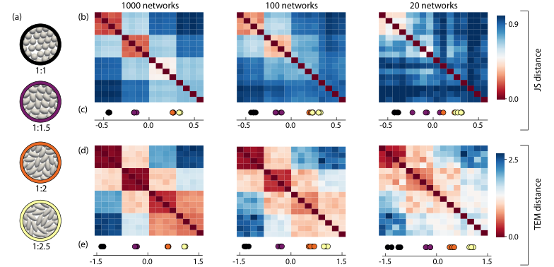
The inability of the JS distance to tell how closely related networks are is a significant drawback when limited data is available. In this regime, the true distribution is not sampled well; while this would reduce the accuracy for all distances, a distance that has no concept of similarity between networks will particularly struggle. To see this, imagine the extreme case where for each distribution we take only the one network that occurs most frequently. The TEM distance may still provide information about the distributions, but the JS distance will give all distances as 0 or 1. To test this intuition, we took jammed disordered packings of 10,000 ellipsoids for aspect ratios 1:1-2.5 (Fig. S11a), and subsampled them, retaining either 1000, 100, or 20 local networks. The TEM and JS distances were calculated (Fig. S11b,d), as were their MDS embeddings, (Fig. S11c,e). The correct MDS embedding is recovered for the TEM distance even when only 20 local networks from each simulation are available, and this is consistent across simulations. For the JS distance, the MDS embedding is incorrect even for 100 local networks. While the correct ordering is recovered for 1000 local networks, there is hardly any separation between the 1:2 and 1:2.5 ellipsoids in the MDS embedding, unlike the 4 clear clusters that are apparent for all TEM MDS embeddings. Therefore, in the case when limited data is available, the TEM distance outperforms the JS distance.
.9 Choice of radius
To capture the local ordering around a point we take the local network of radius . The larger is, the more local information we capture, but also many more distinct networks are observed with corresponding increase in computational cost. Taking the ABP simulations as an example, 320 simulations of 2000 particles were performed, so 640,000 networks were computed in total. For , distinct networks were observed, for , were observed and for , were observed. This means that computing optimal transport exactly for becomes computationally infeasible, but could be solved approximately using entropic regularization Essid and Solomon 2018. However, since contains sufficient information to recover the phase space, the question becomes whether may be sufficient as well. Although taking works to some extent, it is not sufficient to recover the 2D phase space for the ABP simulations, Fig. S12. Using the MDS embedding for , over of the variance is in the first principal component (compared to for ), suggesting, erroneously, that the manifold is 1D, despite the true phase space lying on a 2D manifold.

To understand why taking is insufficient, we calculated the flip graph for all ABP simulations, and calculated the frequency at which each local network was observed (Fig. S13). Neglecting a negligible fraction of the total networks observed (), the flip graph is simply a 1D, or path, graph and the networks tell us only how many neighbors each Voronoi cell has. Euler’s theorem tells us that the average number of neighbors will be 6, and as demonstrated in Fig. S13, the number of neighbors remains close to 6. Therefore, the distribution is approximately 1D; if the fraction of 5 sided shapes is , then the fraction of 7 sided shapes is , and the fraction of 6 sided shapes is , meaning the whole distribution is approximately described by a single parameter. While in reality there are further degrees of freedom, the fact that the distribution is almost 1D explains why will struggle to reconstruct a 2D or higher phase space.
.10 Bacterial swarm
The bacterial strain used for the swarming assay in this study was a comI derivative of the ancestral B. Subtilis strain NCBI3610, obtained from Daniel Kearns’ lab at Indiana University. Cell cultures were grown at 37°C in Luria-Bertani (LB) liquid medium for 18h before incoluation. Swarming plates were prepared by filling of LB medium containing 0.5 bacto agar into a petri dish prior to a drying period of 20 minutes. The plates were then immediately inoculated with a small drop of bacterial culture of volume , which was placed in the center of the plate. Swarms were kept at 37°C in an enclosure containing a water reservoir and imaged for 12h using the automated microscopy routine and setup described in Ref. Jeckel et al. 2019. At each space-time location an image of pixels is taken corresponding to an area of .
To segment the cell centroids, we used the cell segmentation tool Stardist together with a U-Net backbone Schmidt et al. 2018; Ronneberger et al. 2015. For training data, we anually annotated 30 images containing 26,228 cells in total. The following table contains the hyperparameters, if not otherwise stated the default parameters were used.
| parameter | value |
|---|---|
| backbone | U-Net |
| n_rays | 32 |
| unet_n_depth | 3 |
| batch_size | 4 |
| patch_size | (256,256) |
There are 320 experimental snapshots across time and space which, due to the quadratic growth of computing the distance matrix, makes the full MDS embedding expensive (at least the cost of the ABP embedding). The embedding by motif size parameters has no such quadratic cost, and was discussed in the main text. Here we consider instead embedding all snapshots for a fixed time, and hence investigate the spatial structure at a particular time. We performed this embedding for three time points, each containing 15-20 snapshots, Fig. S14. We first note that the swarm is heterogeneous, and the snapshots are separated by or hundreds of bacteria lengths, meaning we do not necessarily expect the properties to change smoothly with radius. While there is often a relationship between the embedding and the radius, the primary principal component does not always correspond to the radius (except for h), Fig. S14. Volume fraction and speed are also strongly linked to the embedding and can explain certain principal components. Finally, we find that the embeddings can cluster phases found by a data-driven clustering of snapshot parameters Jeckel et al. 2019. For the region of the swarm we are analyzing, there are three identified phases: rafting + biofilm precursor (R+BP), rafting (R), and single cell + rafting (SC+R) Jeckel et al. 2019. We find that the phases tend to separate in the embedding, Fig. S14. In addition to phase classification, we can now use the MDS embedding to see if a snapshot is truly representative of its phase or if it is close to transitioning into a different phase.

.11 Geodesics in space
The energetic barrier required to perform a flip in epithelial cell layer suggests that the system might evolve in such a way to minimize the total number of these flips required. To investigate, we seek to find a path between the average start and end experimental distributions that exactly solves this minimization problem. Recall to find the earth mover’s or Wasserstein () distance, we take the start and end distributions, say , and , and solve the for the optimal transport plan moving mass from to . A natural way to interpolate this process would be to instead move mass , from to , for , which results in the intermediate distributions . This path is a geodesic in the sense that , for , but is not the only interpolating distribution to have this property, as geodesics are not unique under the metric Solomon et al.. This distribution could be interpreted as phase separated growth, a fraction of the system is in the initial distribution, the remainder in the final, and the size of the phase in the final distribution grows until the whole system is in that distribution. However, this has a certain unphysical aspect of mass instantaneously appearing in the final state as the path is traversed Solomon et al.. In contrast, it is well known that when computing the second Wasserstein () distance on a continuous manifold , one finds a naturally interpolating path between initial and final distributions. Moreover, the distance can be computed as
| (S5) | ||||
for a probability density over advected by a velocity field, Solomon et al.. The term in the integrand to be minimized is the natural analogue of dissipation for this transport problem, and the intermediate path is the natural interpolation between start and end distributions Solomon et al..
In order to compute a geodesic on a graph, we must find a transport plan , that minimizes
| (S6) |
together with the conservation equation
| (S7) |
with initial and final conditions and ; is the mass transported from to in time . As previously discussed, there are many such that satisfy this equation. Here, we take all transport plans that minimize the cost, and out of these, find the plan that minimizes the transport dissipation. To write down the graph-based equivalent of the transport dissipation, we can interpret the mass transport , so that dissipation would become,
| (S8) |
where the sum is assumed to be taken over non-zero , and denotes the probability density over edge . To define an edge based density (previously density was defined on vertices), we follow Solomon et al., taking the harmonic mean of the densities at the corresponding vertices, . To solve numerically, we discretize in time, finding states, , and transport plans , making the transport dissipation Solomon et al.,
| (S9) |
where the sum over is assumed to only include terms so that , are always non-zero when they appear in the sum. Note that the advective nature of transport is reflected in the harmonic mean by taking the density at the source of the transport at time and the density at the destination of transport at time . The full discretized problem for finding the dissipation regularized geodesic can be stated as
| (S10) | ||||
where the last constraint enforces that the path is still optimal with respect to the metric. The integer parameter determines the level of discritization, with the continuous limit being recovered for Solomon et al.. This problem can be solved by second order conic optimization programs, and whilst significantly slower than solving the linear min-cost flow for , it is still practical for the systems considered here.
We see that the dissipation regularized geodesics calculated by this method closely match the actual path the data takes, unlike the phase separated interpolation, Fig. S15. Fluctuations around the geodesic mean that the system will not exactly minimize dissipation, but nevertheless follows the minimizing path closely.

.12 Topological entropy
In practice, if the underlying parameters are unknown, interpretation of the principal components directly from the data is desirable. In the next section, we introduce tools to analyze the motif size distribution, which yields further interpretations of the embedding. Here, we note that from the observed motif distributions , we can compute the topological Shannon entropy Yoon et al. 2019, . The interpretation of entropy is that it is a measure of how many states are available to the system. The entropy often explains the first MDS principal component, for instance in the ABP embedding, Fig. S16. In the Drosophila example, the entropy corresponds to the first principal component, notably decreasing with time, Fig. S16, consistent with known results about the increasing regularity of the developing wing Etournay et al. 2015.

.13 Tracy-Widom distribution
We seek to understand the structure of the data by understanding the probability distribution of motifs. This space is hard to analyze directly, so we consider a projection onto , by taking the distribution of motif sizes, defining the size of a motif to be the number of vertices that it has. In the main text, we claimed that for the swarm data, the distributions differed in mean and variance, but all lay on a universal distribution, namely the Tracy-Widom (TW) distribution. Here we provide stronger numerical evidence that the distribution is indeed TW by analyzing the network formed by a Poisson point process, known as a Poisson-Voronoi (PV) tesselation Lazar et al. 2013, which is equivalent to a non-interacting gas, taking points in a periodic domain. To analyze the motif size distribution, we took the observed distribution for fixed , and rescaled so that it has mean 0, variance 1. We compare this against various known distributions including a Gaussian, Log-normal, and TW for all parameters, all rescaled to have unit variance and zero mean. The distribution were chosen for their universal characteristics, and hence plausible appearance in the motif size distribution. Gaussian distributions are universal due to the central limit theorem, and for positive variables a Log-normal distribution has universal properties Limpert et al. 2001. We discuss in the main text the universal character of TW distributions. The parameters for the Log-normal were chosen by maximum likelihood estimation before rescaling, the TW and Gaussian distributions were only rescaled, not fitted. We see for , that the distribution lies enough close to TW to be plausible, but differs slightly in the left tail and due to the discrete nature of motif sizes, does not finely resolve the distribution, Fig. S17a. However, by taking ever larger motif sizes, , the observed distribution gets significantly closer to TW, matching in both the regions and in the tails until at least probability density , Fig. S17b-c. In particular, the distribution for larger motif sizes lies on TW, and not a Gaussian or Log-normal, even though Log-normal (for our parameters) and TW are very similar distributions. TW with appears to be the best fitting of the TW distributions, although they only differ slightly when rescaled, so further numerical tests would be needed to confirm this. In the main text, and the rest of this document we use for the TW distribution. We note that this distribution is universal in the sense that the motif size distributions for PV and for the swarm data do not share the same mean or variance, and the underlying processes are different. The mean motif size of a PV process is 20.7 and variance 14.8, which is significantly greater than the corresponding quantities measured from the swarm snapshots. Further, PV can be thought of as a snapshot of an non-interacting ideal gas, whereas the bacteria in the swarm have strong excluded volume interactions and density plays an important role. Nevertheless, the same distribution is found.
.14 Analysis of motif size distribution
Applying the motif size analysis to the ABP data, we find a range of possible distributions, Fig. S18d,
not all of which appear to be TW. We can approximately characterize these distributions by taking their mean,
variance, and third moment. We find that the mean and variance correspond to the first principal component of the MDS
embedding, and the third moment corresponds to the second principal component, Fig. S18(a-c). In an alternative
to the TEM-MDS embedding, one can plot the simulations in the variance-third moment plane, finding that this again recovers the
activity/volume fraction phase space, Fig. S18(e-f).
This is not preferable to the metric embedding, since there is no notion of distance,
although here one need not compute components of a distance matrix, providing an
alternative when is large. To understand these embeddings, we see that reducing the volume
fraction for fixed activity causes more states to become available as particles interact less. Hence the motif size variance
increases and so does the third moment (as does the topological entropy). Interestingly, when the activity is increased,
the variance does not change much, but the third moment increases significantly. In the most extreme case of ,
going from the lowest activity to the highest, the third moment increases by a factor of 16, whereas the variance increases
by a factor of 1.2, and the mean does not chance. Hence activity changes the distribution
by increasing the probability of large motif fluctuations,
which directly correspond to the giant number fluctuations of the phase separated regime Fily et al. 2014.

The distributions seen in the ABP simulations appear to take a variety of forms, although the Tracy-Widom (TW) distribution appears, Fig. S19. We evaluate where in the parameter space the motif distribution appears most TW like, by comparing the distribution rescaled to zero mean and variance 1, and the TW distribution similarly scaled. We use the Kullback-Leibler (KL) divergence between two distributions, defined as , representing the amount of information lost when the data distribution () is approximated by the TW distribution (). To compare continuous and discrete distributions in calculating the KL divergence, we consider the discritized TW pdf to be the mass lying within a bin as defined by the histogram of the discrete data. We find that in the most active regimes the observed distribution is furthest from TW. Perhaps this is because in the phase separated regimes, the dense phase is a strongly coupled glass like phase, with a narrow distribution of motif sizes, but the gas-like phases can take a wide variety of motif sizes, leading to unusual distribution tails. The region where the distribution is closest to TW, is the region where the system is most liquid like.
For the Drosophila data, we find that the motif size distribution is well approximated by TW in early times, whilst the EC layer is irregular and the system is most liquid-like. However, at later times when the final state of a more regular lattice appears, the distribution is no longer close to TW, Fig. S20.
For the bacterial swarm data, while the motif distributions have varying mean and variance, the distributions appeared to have a common form when rescaled to have 0 mean and variance 1, Fig. S21a. We rescale every observed motif by the mean and variance of the distribution at that snapshot and combine in a single histogram. Since all distributions have similar mean, and are originally defined on the integers, the combined histogram still shows discrete peaks, Fig. S21b. We therefore choose histogram bins so that each contains exactly one discrete spike, and plot them as points so that the height represents the probability density, the location represents the center of mass, with horizontal bars of representing the width of the peak. We compare this against various known distributions, Fig. S21(c-d), as before with the PV tesselation. We once again find that TW fits the data well, although since we are using here, they disagree slightly at the left tail.
References
- Aurenhammer et al. (2013) F. Aurenhammer, R. Klein, and D.-T. Lee, Voronoi Diagrams and Delaunay Triangulations, 1st ed. (World Scientific Publishing Co., Inc., River Edge, NJ, USA, 2013).
- Edelsbrunner et al. (1983) H. Edelsbrunner, D. Kirkpatrick, and R. Seidel, IEEE Trans. Information Theory 29, 551 (1983).
- Etournay et al. (2015) R. Etournay, M. Popović, M. Merkel, A. Nandi, C. Blasse, B. Aigouy, H. Brandl, G. Myers, G. Salbreux, F. Jülicher, and S. Eaton, eLife 4, e07090 (2015).
- Weinberg (1966) L. Weinberg, IEEE Trans. Circuit Theory 13, 142 (1966).
- Lazar et al. (2012) E. A. Lazar, J. K. Mason, R. D. MacPherson, and D. J. Srolovitz, Phys. Rev. Lett. 109, 095505 (2012).
- Bose and Hurtado (2009) P. Bose and F. Hurtado, Comput. Geometry 42, 60 (2009).
- Wagner and Lowrance (1975) R. A. Wagner and R. Lowrance, J. ACM 22, 177 (1975).
- Essid and Solomon (2018) M. Essid and J. Solomon, SIAM J. Sci. Comput. 40, A1961 (2018).
- Tenenbaum et al. (2000) J. B. Tenenbaum, V. d. Silva, and J. C. Langford, Science 290, 2319 (2000).
- Fily et al. (2014) Y. Fily, S. Henkes, and M. C. Marchetti, Soft Matter 10, 2132 (2014).
- Mason et al. (2012) J. K. Mason, E. A. Lazar, R. D. MacPherson, and D. J. Srolovitz, Phys. Rev. E 86, 051128 (2012).
- (12) J. Solomon, arXiv:1801.07745 .
- Jeckel et al. (2019) H. Jeckel, E. Jelli, R. Hartmann, P. K. Singh, R. Mok, J. F. Totz, L. Vidakovic, B. Eckhardt, J. Dunkel, and K. Drescher, Proc. Nat. Acad. Sci. 116, 1489 (2019).
- Schmidt et al. (2018) U. Schmidt, M. Weigert, C. Broaddus, and G. Myers, in Medical Image Computing and Computer Assisted Intervention – MICCAI 2018, edited by A. F. Frangi, J. A. Schnabel, C. Davatzikos, C. Alberola-López, and G. Fichtinger (Springer International Publishing, Cham, 2018) pp. 265–273.
- Ronneberger et al. (2015) O. Ronneberger, P. Fischer, and T. Brox, in Medical Image Computing and Computer-Assisted Intervention – MICCAI 2015, Lecture Notes in Computer Science, Vol. 9351 (Springer, 2015) arXiv:1505.04597 .
- (16) J. Solomon, R. Rustamov, L. Guibas, and A. Butscher, arXiv:1603.06927 .
- Yoon et al. (2019) T. J. Yoon, M. Y. Ha, E. A. Lazar, W. B. Lee, and Y.-W. Lee, Phys. Rev. E 100, 012118 (2019).
- Lazar et al. (2013) E. A. Lazar, J. K. Mason, R. D. MacPherson, and D. J. Srolovitz, Phys. Rev. E 88, 063309 (2013).
- Limpert et al. (2001) E. Limpert, W. A. Stahel, and M. Abbt, BioScience 51, 341 (2001).