Detection of WHIM in the Planck data using Stack First approachBased on observations obtained with Planck (http://www.esa.int/Planck), an ESA science mission with instruments and contributions directly funded by ESA Member States, NASA, and Canada.
Abstract
We detect the diffuse thermal Sunyaev-Zeldovich (tSZ) effect from the gas filaments between the Luminous Red Galaxy (LRG) pairs using a new approach relying on stacking the individual frequency maps. We apply and demonstrate our method on LRG pairs in the SDSS DR12 catalogue selected with an improved selection criterion that ensures minimal contamination by the Galactic CO emission as well as the tSZ signal from the clusters of galaxies. We first stack the Planck channel maps and then perform the Internal Linear Combination method to extract the diffuse signal. Our Stack First approach makes the component separation a lot easier as the stacking greatly suppresses the noise and CMB contributions while the dust foreground becomes homogeneous in spectral-domain across the stacked patch. Thus one component, the CMB, is removed while the rest of the foregrounds are made simpler even before component separation algorithm is applied. We obtain the WHIM signal of in the gas filaments, accounting for the electron overdensity of . We estimate the detection significance to be . This excess signal is tracing the warm-hot intergalactic medium and it could account for most of the missing baryons of the Universe. We show that the Stack First approach is more robust to systematics and produces a cleaner signal compared to the methods relying on stacking the -maps to detect weak tSZ signal currently being used by the cosmology community.
1 Introduction
According to the standard CDM model of Cosmology, our Universe is composed of approximately baryonic matter with the rest of the total energy density in the form of dark matter and dark energy. The current most precise measurement of the baryonic energy density parameter, , where and is the Hubble constant, is derived from the cosmic microwave background (CMB) measurements (Plank_Colab_cosmopara) and thus tells us the amount of baryons present at the time of recombination at redshift (zks68; peebles68). However, observations of the low redshift Universe show that the baryon fraction today falls below the expected universal value from CMB for almost all regions (except for the massive haloes) (McGaugh_2009). It has been known for sometime now that almost all of the baryons at high redshifts () are accounted for in the Lyman- absorption forest (Weinsberg_1997). In contrast, at low redshifts () we see that even after accounting for the baryons in stars, galaxies, Lyman- forest gas along with broad Lyman- and absorbers, and hot gas in clusters of galaxies, almost half of the baryons are still missing (Shull_2012). This apparent discrepancy between the direct observations spanning the electromagnetic spectrum from radio to X-rays and the predicted baryonic mass in the standard model of cosmology and the galaxy formation theories need to be resolved by locating ‘the missing baryons’.
The gravitational instability of small initial Gaussian density fluctuations results in anisotropic collapse (Zeldovich_1970; shz1989) forming sheets (Zeldovich pancakes) and filaments that make up a web like structure, the cosmic web (ks1983; defw1985; gh1989; 2df_survey; gott2005; mil2005). Galaxies and galaxy clusters, embedded in the knots of the web (also known as dark matter haloes), are therefore connected by large-scale filamentary structures. It has been long known from simulations that a large fraction of the baryons are in the seemingly empty regions of the universe, i.e. outside the gravitationally bound haloes (cen). The haloes are highly overdense regions, but there are regions which are mildly overdense but span a much larger volume. These relatively low density and high volume spanning regions of sheets and filaments could be a rich reservoir of the missing baryons as they go undetected by the conventional methods. The gas in these filaments or the intergalactic medium (IGM) have a density of the order of ten times the mean baryon density and temperatures between K. Hydrodynamical simulations suggest that this warm hot intergalactic medium (WHIM) could contain of all baryons today (Cen_2001; Dave:2001), even though the filaments occupy only of the total volume (Cautan_2014). The high ionization degree would have prevented these baryons from being detected in absorption line surveys in the radio and optical bands while the low density and temperature would have prevented them from being detected in either emission lines or in the X-ray surveys targeting thermal X-ray emission, making them an ideal candidate for the missing baryons. The efforts for the detection of these missing baryons have been ongoing. Most of the campaigns targeting WHIM have focused on the detection of hot gas using X-rays from individual filaments (xrayfail) or from the absorption spectra of quasars (Shull_2012). These methods are however able to probe only a part of the phase space of WHIM leaving about of the baryons still unobserved (Shull_2012; Nicastro:2017). There has been a recent work on X-ray detection of filamentary structures near cluster Abell 2744 Eckert:2015, albeit their work probes the hotter and denser end of the WHIM, and quote a small fraction of baryons in that state. Recent observations of OVII absorption lines in the X-ray spectra of a blazar provide some evidence for a significant fraction of baryons to be present in gas at nkk2018 leading to the claim by the authors that the missing baryons have been found, albeit in just two systems very close to a single blazar. There have been detections of kinetic Sunyaev Zeldovich (kSZ) effect from the baryons in the dark matter halos (galaxies and clusters of galaxies) Hernandez:2015; Hill:2016; Schann:2016; Bernardis:2017, which is sensitive to peculiar motion of the baryons with non zero velocities. Recently, it was shown that the cross-correlation of angular fluctuations of galaxy redshifts with the kSZ effect in CMB temperature maps Jonas_2019 can be sensitive to baryons in regions with overdensities consistent with those of the filaments and sheets in the cosmic web.
The elastic scattering of hot free electrons in the WHIM with the CMB photons boosts the energy of the CMB photons resulting in a characteristic spectral distortion of the CMB, the thermal Sunyaev Zeldovich (tSZ) effect (sz1969). The tSZ effect provides a way to study WHIM through multifrequency experiments, such as Planck, which can separate the tSZ effect from the CMB and foreground emissions (Planck-A22:2016; hs2014; Khatri:2016). The magnitude of tSZ distortion, denoted by , is a function of both the gas density and the temperature of the medium (Sunyaev:1972) and is given by (using Planck 2018 cosmological parameters planck2018 and fully ionized primordial gas)
| (1) |
where is the free electron number density, is
the electron temperature, is the Thomson cross section, is
the Boltzmann constant, is the mass of electron, is the speed of
light, the integral is over the line of sight distance, , through the
WHIM, is the overdensity, is the filament
baryon density, is the average baryon density, is the
length of filament along the line of sight and is the Thomson optical depth through the WHIM or the
filament along the line of sight. If we take the filament baryon density to be
average baryon density (), we get an optical depth of at . For a temperature of ,
we will get a tSZ
signal of or a Rayleigh-Jeans temperature decrement
of after integrating over Mpc along the line of sight. This signal is much smaller than the
noise in the current best CMB experiments, and in particular much smaller compared
to the sensitivity of Planck. Therefore, it is not possible at present to
detect the individual filaments. We can however beat down the noise by
stacking hundreds of thousands of filaments, improving the signal to noise
ratio, , by a factor of hundreds. The signal from the WHIM in the
stacked objects would be detectable in the Planck data if we can remove the
contamination from the CMB as well as Galactic foregrounds with the same
accuracy.
The approach of stacking to improve the has been used previously to detect the faint tSZ signatures. The stacking of the tSZ signal in the maps released by the Planck collaboration (Planck-A22:2016) on the positions of known galaxy pairs of massive luminous red
galaxy (LRGs) (Tanimura:2019, hereafter T19) as well as constant mass (CMASS) galaxy
samples
(Graaff:2019, hereafter G19) from the Sloan Digital Sky Survey (SDSS) has been
performed in an effort to find the missing baryons. In this
technique, the selected close galaxy pairs within a certain radial and
tangential distance are stacked up coherently in the map
created from the Planck data by a component separation algorithm. G19
claim a detection of around of the baryons with
detection of the tSZ signal,
leaving of the baryons still unaccounted for. A
stacking of tSZ maps around superclusters was done in
Tanimura_19_intercluster, in which the authors claim a
detection of of missing baryons in the intercluser gas in
superclusters with the tSZ effect detected at significance.
We present a new algorithm for detection of WHIM through tSZ effect in multifrequency CMB data sets. Although the individual steps of our algorithm are similar to T19 and G19, the order in which the steps are performed is completely new. It turns out that just reordering the steps makes a huge difference. The main essence of our algorithm is to first stack the individual frequency maps at source locations and then extract the component from the multifrequency stacked data using standard component separation algorithms. Our new algorithm is motivated and described in Sec. 2. In Sec. 3, we introduce the Planck data products and the sky masks used in this paper. Section 4 introduces the main data analysis part of the paper to extract the signal at the location of LRG pairs from the stacked Planck maps. The modelling of signal expected from individual halo contribution and its subtraction from the total signal to see the signature of WHIM in the filament region is discussed in Sec. 5. In Sec. 6, we discuss the null test and the error estimate of the excess signal. Finally we present our conclusions in Sec. 9.
2 A new algorithm to detect weak tSZ signals in Planck data
In the previous attempts at detecting the WHIM through tSZ effect Tanimura:2019; Graaff:2019, there is ambiguity as to what might be the true signal. In the conventional method, stacking of sources is done on preprocessed publicly available Planck maps obtained from Needlet Internal Linear Combination (NILC) (Remazeilles:2011) and Modified Internal Linear Combination Algorithm (MILCA) (Hurier:2013) algorithms. The residual contamination by the other foreground emissions (dust, CO, free-free, synchrotron and CMB leakage) after component separation in the maps is much larger compared to the signal we are interested in (AHD2015; Khatri:2016). Thus, when we stack a large number of galaxy pairs, there will be some cancellation between the positive and negative contamination leaving a net residual systematic which can be either positive or negative. This can be seen in the probability distribution functions (PDFs) of in NILC, MILCA and Linearized Iterative Least-squares (LIL) maps in Fig. 1 for the pixels which lie in-between the galaxies in a galaxy pair. The selection procedure is explained in the next section. We see that there is significant positive as well as negative excess over the Gaussian noise. The negative excess is contamination while the positive excess is contamination + signal. In particular, the contamination signal is more than a factor of 100 larger compared to the signal we are interested in. There is no guarantee that the positive contamination is equal to the negative contamination, and there would be large unknown systematic bias in the signal obtained in this way.
We propose a new method of extracting the signal from the filaments connecting the galaxy pairs. We begin by first stacking the individual Planck frequency maps at the positions of the LRG pairs. We then perform the component separation using Internal Linear Combination (ILC) (tegmark1996; tegmark1998; Bennett:2003) algorithm on the stacked frequency maps to extract out the signal. By doing stacking first and component separation later, we achieve a number of advantages over the conventional method of stacking the map (Tanimura:2019; Graaff:2019):
- 1.
We suppress the instrumental noise before doing ILC. Thus even the noisy 70 GHz and 100 GHz channel are utilized efficiently. In conventional method, these channels are down-weighted as the ILC tries to strike a compromise between reducing noise and reducing foregrounds in the final map.
- 2.
The Gaussian random CMB fluctuations, uncorrelated with the positions of the galaxies, are suppressed. Thus we have one less component even before we begin the ILC.
- 3.
Since Galactic foregrounds are also uncorrelated with the galaxy positions, by stacking the frequency maps, we are homogenizing the foregrounds in amplitude as well as in spectral shape across our stacked patch. That is, in every pixel in the final stacked map after stacking patches of interest from different parts of the sky, we should expect a sum of foreground contamination from a large number of sources, essentially sampling the whole foreground parameter space. Every pixel should end up with a very similar foreground contribution, effectively summing the complicated foregrounds comprising of many different components varying across the sky to a single foreground component across our patch.
The full power of ILC is therefore concentrated in eliminating the foregrounds, as noise and CMB is eliminated in the pre-ILC stage. The foreground spatial structure is also simplified by stacking the frequency maps. In particular, the dust emission has spectrally smooth behaviour in the stacked frequency images, with negligible variation across the image, as a result of averaging. In our approach, since we are suppressing noise before doing ILC, we can work at higher resolution compared to the conventional method. We will demonstrate this by doing analysis at resolution although most of our results would be derived at resolution.
3 Data and masks
3.1 SDSS and Planck data

We use SDSS data release 12 (DR12) with the same criteria as T19 to make a catalog of LRGs with stellar mass (Prakash:2016). We take the stellar mass estimate based on a principal component analysis method from (Chen:2012). Next, we construct a sample of LRG pairs with the radial distance between the galaxies of a pair Mpc and the tangential distance in the range Mpc. We adopt a CDM cosmology with , , and Mpc-1 for calculation of the comoving distances from the redshift () information. If two or more LRG pairs fall within 30′ in the projected sky coordinates (Galactic latitude and longitude), then we only keep the higher average mass LRG pairs in the sample. We find roughly LRG pairs satisfying both of the distance criteria in the SDSS DR12 sample. The angular separation between the selected LRG pairs lies between 19′ and 203′ .
We will use the Planck 2015 intensity maps from 70 to 857 GHz and IRIS 100 m (or 3000 GHz) map (MAMD-IRIS) for our analysis. The temperature data has not changed significantly between 2015 and 2018 releases. We rebeam the Planck HFI maps to a common beam resolution of 10′ full width half maximum (FWHM), taking into account the effective beam function of each map and reduce to a HEALPix resolution of from the original to make computations faster. While smoothing to 10′ beam resolution, we only retain the scales up to for Planck HFI channels and for Planck 70 GHz LFI channel. As a validation step, we also produce Planck maps at a common beam resolution of 8′ FWHM with for Planck HFI channels and keeping 70 GHz LFI channel .
We will use the MILCA and NILC maps from the Planck Legacy Archive11 1 https://www.cosmos.esa.int/web/planck/pla for comparison. The MILCA maps were produced using all of the Planck High Frequency Instrument (HFI) intensity maps ( GHz). The NILC method uses in addition the Low Frequency Instrument (LFI) data () GHz) at large angular scales (). The angular resolution of both of these maps is 10′ FWHM. We downgrade the original maps from (pixel size=1.7′) to (pixel size=3.4′) for computational efficiency.
3.2 Sky masks and sample selection
We will use the sky mask obtained in (Khatri:2016, hereafter K86 mask) specifically for the tSZ studies with an unmasked sky fraction as the baseline. This mask specifically tries to minimize the CO line emission contamination and also covers strong point sources. We will also use the masks provided by the Planck collaboration, in particular the Galactic + point source mask with (henceforth PL48 mask) to compare with the T19 results.
As we estimated in the last section, we expect the IGM in the filaments between the galaxies to give a very weak tSZ signal, much below the noise level of the Planck for individual objects. Thus, in addition to the regions of strong CO line contamination (Khatri:2016), we also want to avoid the strong tSZ signal coming from much hotter and denser gas in the clusters of galaxies in the foreground or background, i.e. we want to select only those pairs of galaxies for which, in the individual objects, the signal is undetectable and we are dominated by the instrumental noise. To accomplish this, we use the fact that CO emission is also a weak signal in the Planck data, of similar strength to the signal but with a different spectrum. We can fit a model consisting of CMB + Dust + tSZ signal to the Planck HFI data as well as a model consisting of CMB + Dust + CO emission, and compare the of the two models (which have the same number of parameters). In the regions where CO emission is stronger than the tSZ, we will have smaller for the CO model and the difference between the for the two models will be negative. In the opposite case, when we have stronger tSZ signal, will be positive. We want to avoid both these cases. We want to select galaxies such that we are noise dominated and unable to distinguish between the two models, i.e. . These model fits were performed in Khatri:2016 and we will use the map obtained in Khatri:2016 to further prune our galaxy sample. For each LRG pair, we attribute a value by computing the average of the sky pixels that lies within 20′ radius from the centre of LRG location. We have of our sample with a and of our sample with a . We can thus use aggressive thresholds in removing the most contaminated galaxy pairs but still loose only a small fraction of the sample.
We first extend the K86 mask by masking the sky pixels where the values are either highly negative or highly positive, i.e. . This extended K86 mask, hereafter eK86, is shown in Fig. 2. This extension masks the Planck detected 1653 clusters (Planck-A27:2016), SZ dominated regions and molecular clouds from our concerned sample. If either of the two LRGs of the pair falls in the masked region, then we exclude that LRG pair from our stacking analysis. The PDF of average for all galaxy pairs in our sample, after applying the eK86 mask, is plotted in Fig. 3. The skewness towards positive values in the distribution of with eK86 mask towards the positive side shows that in the concerned sky regions signal dominates over the foreground CO emission. To get an even cleaner sample, we further eliminate the galaxies in the tails of the PDF and consider only those LRG pairs for stacking for which , marked by vertical lines in Fig. 3. We can get cleaner samples by further reducing the threshold. Also in order to test that the threshold does not affect our results, we will consider samples with thresholds of containing 144930, 128528, 113374, and 88001 LRG pairs respectively. We show in Fig. 4 the distributions of mean mass () and mean redshift of the LRG pairs for the four thresholds. We see that the mass and redshift distributions are insensitive to the thresholds. The thresholds, therefore, do not introduce any bias in our sample.
4 Stacking analysis
We use the following procedure to stack the Planck sky maps at each frequency. The angular separation between the LRG pairs in our sample spans from 19′ to 203′. We first project a given LRG pair from the spherical coordinates onto a normalized tangent plane centered at the midpoint of the line joining the pair such that one LRG is placed at and the other LRG at (Clampitt_2016). We interpolate the tangent plane projections of all the LRG pairs to an equal size grid. For our analysis we project the tangent plane to a grid of pixels. The angular resolution of each pixel in the grid concerned varies from pair to pair. The two LRGs are always placed 50 pixels apart in the grid, the pixel resolution varies from for the pair with least angular separation to for the largest. We then stack on the equal sized grids. We interchange the one LRG location from to and other vice versa to produce the symmetric stacked signal on both LRG positions. We perform the stacking for the four selected samples as discussed in the previous section for all of the Planck HFI maps and the 70 GHz LFI map at 8′ and 10′ FWHM resolutions. We note that these are slightly finer compared to the native 70 GHz channel resolution and therefore the noise in 70 GHz maps gets boosted. However, the noise is suppressed again when we stack and we can thus hope that the 70 GHz channel (as well as 100 GHz channel at 8′) will contribute to the signal.
We show the stacked Planck frequency maps in Fig. 5. The stacked maps show an increase in foreground contamination as we increase the thresholds from 0.05 to 0.2. We see the unmistakable signatures of the hot gas in the filament region due to the tSZ effect in Fig. 5, i.e. a negative signal at 143 GHz and lower frequencies with respect to the average ambient background around the galaxies and a positive signal for GHz. This signature becomes slightly less prominent for higher thresholds. We will be using our cleanest sample with for our baseline analysis. The signal at the position of galaxies is dominated by the radio and infrared emission from the galaxies themselves. We expect this galactic contamination to become subdominant as we go away from the centers of the galaxies to the intergalactic medium. We fit the modified blackbody spectrum to every pixel in the stacked image from 217 to 3000 GHz. The dust temperature in the fit is fixed to 18 K. The fitted dust amplitude normalised at 353 GHz has the same morphology as the 353 GHz stacked Planck map. After taking into account the color correction factors due to the Planck bandpasses, the fitted dust spectral indices are close to 1.4 over the entire stacked patch. We can conclude that the dust emission has spectrally smooth behaviour as a result of averaging of dust spectral energy distribution over the different line of sights. We will need to remove the galactic contamination from the LRGs themselves to get an unbiased estimate of the signal from the intergalactic medium.

4.1 Blind component separation
We will use the ILC method (tegmark1996; tegmark1998; Bennett:2003) on the stacked Planck maps to extract the signal. The ILC is a blind component separation method used to extract the signal of interest, whose spectrum is known, from multifrequency observations without assuming anything about the frequency dependence of unwanted foreground contamination. It has been used extensively in the CMB data analysis in the past to extract the CMB signal from multifrequency Wilkinson Microwave Anisotropy Probe (WMAP) sky observations. The ILC method can be applied over distinct regions of the sky in pixel space (Bennett:2003; Eriksen:2004), domains in harmonic space (Tegmark:2003), or domains in needlet space (Basak_NILC_2012). The NILC and MILCA component separation methods used by the Planck collaboration to extract the signal from the multifrequency Planck maps are also based on the ILC method with additional constraints (Remazeilles:2011; Hurier:2013).
The ILC is a multifrequency linear filter that minimizes the variance of the reconstructed map. We assume the stacked maps () in each Planck channels as a superposition of signal, foreground () and noise (), written as , where the index labels the pixels in the stacked map. The coefficients contains the relative strength of the signal in the different Planck channels. The ILC solution for the tSZ signal, is given by . The weights, , are found by minimizing the variance of subjected to the constraint that the signal is preserved, i.e. (Remazeilles:2011; Hurier:2013).

We use the ILC method in pixel space to reconstruct the stacked signal from the stacked Planck maps. We show the map for our four LRG pair samples with different thresholds and using different frequency channel combinations in Fig. 6.
The ILC maps are quite robust w.r.t to the changing thresholds as well as the number of frequency channels. We will use the reconstructed ILC map derived from the frequency range GHz for our fiducial analysis. The ILC weights obtained from our analysis with K86 mask and selection criterion are quoted in Table 1 and compared with the ILC weights obtained for unstacked maps. We see from Fig. 6 that removing 70 GHz and/or 545 GHz channels does not make a significant difference, implying that the ILC has converged as far as the number of frequency channels is concerned. The strong signal at the galaxy positions is indicative of residual contamination from the emissions of the stacked galaxies themselves which needs to be estimated and removed.
Since we are doing ILC on a small number of pixels, there maybe ILC bias coming from chance correlations between the noise, signal, and foregrounds tegmark1996; dc2007; dc2009. To check for the ILC bias we half the size of the patch around the LRG pairs from arcmin to arcmin and the number of interpolated pixels from to . The results of comparison are shown in Fig. 7. We also do the analysis at original HEALPix resolution of . We see no significant evidence for ILC bias. At higher resolution of , the signal is a little smoother, but otherwise consistent with results.
We also validate our stack first approach on simulations of realistic sky simulations in Appendix A and show that our stack first + ILC approach recovers the WHIM tSZ signal without bias or significant foreground contamination. We note that since we are not interested in the mean background signal, we implement the standard ILC in which the cost function that is minimized is the variance of the reconstructed map Eriksen:2004; dc2007 i.e. the fluctuations about the mean are minimized. There are other choices for the cost function possible. An alternative cost function proposed in Khatri_FCILC_2019 minimizes L2 norm of the total signal, including the average signal, especially useful when we are interested in the large scale modes. We tried both formulations and found that the two choices of the cost function give consistent results, with the standard ILC giving a slightly stronger detection significance. The fact that the two formulations give results which are similar can be taken as additional evidence that the foregrounds are getting homogenized by stacking as expected.

| Frequency | ILC weights | ||
|---|---|---|---|
| in GHz | with K86 | PL48 mask | Unstacked pixels |
| 70 | |||
| 100 | 0.0182 | ||
| 143 | |||
| 217 | 0.5861 | 0.1518 | 0.2444 |
| 353 | 0.0465 | 0.0352 | |
| 545 | 0.0012 | ||
4.2 Component separation by parameter fitting
In order to use parameter fitting to do component separation, we need an accurate model. However stacking on frequency maps mixes different foreground spectra, in particular mixes dust, CO and low frequency emission. It is therefore difficult to come-up with a foreground that will be accurate enough for our purpose. However, we can still use parameter fitting to learn about the foregrounds and check our assumptions. In particular, we want to check whether the foreground shape is really homogenized over our patch by stacking and that any residual foreground contamination is morphologically different from the SZ signal we are interested in. We employ LIL parametric fitting algorithm developed in (k2015; Khatri:2016). We fit a simple parametric model consisting of either CMB + dust + tSZ or CMB + dust + CO components to 4 HFI channels from 100 GHz to 353 GHz. We model dust by a modified blackbody spectrum with fixed temperature and fixed line ratios for CO line contribution in different channels, following (Khatri:2016). The parameters to fit are CMB temperature, tSZ or CO amplitude, dust amplitude and the dust spectral index.
The results of the parameter fitting exercise are shown in Fig. 8. The top panel shows the fitted SZ signal, the CO signal and the dust amplitude (for SZ+dust+CMB model fit) signal. In the bottom panel, we have removed the average background to show the fluctuations. We recover the signal with morphology remarkably similar to the ILC method. We also see that both the dust and the CO signals are quite homogeneous. Comparing the top and bottom panels, we see that the dust amplitude is almost homogeneous over the entire patch with fluctuations of . For the CO signal also, the fluctuations are smaller by a factor of compared to the average signal. In particular the CO fluctuations are dominated by noise and are also statistically homogeneous and random, apart from the small leakage from other components at the locations of the galaxies. In particular the CO signal fluctuations are of order few which corresponds to few in CMB temperature units at 100 GHz (see planckhfi; k2015, for conversion factors). This is approximately the amplitude of the noise after stacking galaxies in the most sensitive Planck maps with full sky map level sensitivity of hfi2016; hfi2018.
We note that CO is already a very weak contamination in Planck maps (see also Appendix A). We also note that while doing standard ILC Eriksen:2004; dc2007, we subtract out the average or the monopole part of the signal. Thus of the dust and most of the CO contamination would be subtracted out even before we do the ILC. Most of the background SZ signal, seen in the top panel, will also be suppressed. The small correlation in the CO map with the galaxy positions is because when we fit for the CO, our model does not include the SZ component. The SZ component will therefore contaminate all other components and will show up prominently in the weakest component which is the CO k2015. However, even in CO, the SZ contamination is at the level of noise fluctuations in the rest of the map. Most of the foregrounds will thus be removed and suppressed even before we have applied the ILC. The ILC should remove any remaining CO and dust foregrounds from the stacked maps bringing down the contamination to the noise levels. In particular the ILC is most efficient in removing the foregrounds in noiseless maps (see dc2007, for proof and detailed study of ILC methods). Stacking before ILC suppresses the noise thus increasing the efficiency of foreground removal. We must still account for the residual contamination and SZ signal from the stacked galaxies themselves. This is however not a big concern. Since the galaxies themselves would be unresolved at Planck resolution, the dust and SZ signals from the galaxies is well approximated by two non-overlapping Gaussian discs and subtracted.
With the parameter fitting exercise, we have therefore quantified the benefits of the Stack First approach. We have shown that we have a factor of 1000 suppression in the fluctuating part of the foregrounds, in addition to the suppression of noise, by just stacking the individual frequency maps even before the ILC component separation algorithm is applied.
5 Excess signal
We expect two symmetric peaks in the stacked ILC map as we stack the Planck frequency maps twice by interchanging the LRG positions. The position of the LRGs may have some remaining dust contamination, since the LRGs themselves are expected to have strong dust emission (as evident by the lower panels in the first column of Fig. 5) and even a small leakage may be significant compared to the tSZ signal. However, the region between the LRGs, where we expect to find the WHIM, is relatively free of dust and leakage from any weak dust emission from the intergalactic medium would be suppressed even further by the ILC. The middle panel of Fig. 9 shows the profile of the stacked ILC map along Y=0 axis. The stacked ILC signal for our baseline case has the dominant contributions from the individual LRG halo. The circular model for halos is a good approximation since most of our galaxies are unresolved and any non-circular beam effects will get symmetrized when stacking a large number of objects. T19 have shown that other systematic effects are also small. To extract the excess signal in the filament region connecting the LRG pair, we need to subtract the individual LRG halo contribution.

We exclude the central region and fit a Gaussian model to the single-halo signal on both the sides (Tanimura:2019). The blue solid line in the middle panel of Fig. 9 is the best-fit Gaussian model to the data, excluding the central LRG region from . The 2D circular Gaussian model is constructed based on the fit to the data at . The residuals after fitting the best-fit 2D circular Gaussian model along the Y=0 and X=0 are shown in the bottom panel of Fig. 9. The map representation of the same is shown in the top panel of Fig. 9. The amplitude of the excess signal is in the region at Y=0. The excess signal peaks in the central filament region between and . The average of the excess signal in the central filament region is , which is approximately a factor of three higher than the value reported in T19.
We note that our basic selection criteria is same as T19 however we impose additional thresholds to further prune our samples, making our results more robust to accidental contamination by foreground or background clusters. In order to relate the measured signal to the filament properties, we use the following density profile for the filament similarly to T19,
| (2) |
where is the electron number density of a filament at redshift and distance from the filament center along the line of sight, is the core radius of the filament and we will take Mpc. The density profile is set to zero at . The mean electron number density as a function of redshift, is given by , where is the baryon density parameter, is the critical density of the Universe today, is the proton mass and is the mean molecular weight of primordial plasma with hydrogen by mass. We also define the overdensity at the center of the filament as . We assume Planck CDM cosmology planck2018 giving average electron number density today to be . The electron number density in filaments, can be expressed in terms of overdensity by multiplying and dividing Eq. 2 by as
| (3) |
Assuming a constant electron temperature and a symmetry along the filament axis, we can express as a line of sight integration of the filament density profile () as,
| (4) |
where is the cut-off radius of the filaments and is the parameter for line of sight integration. The mean redshift of each LRG pair in our sample is known. On averaging over all LRG pairs in our fiducial sample, we obtain the average excess signal from the filament for our sample as
| (5) |
As the WHIM constitutes a major chunk of the matter in the filaments (Martizzi_Illustris:2019), we can assume an average temperature of K in order to estimate the density contrast of the filament from the signal. This electron temperature is within the upper bounds obtained from IIlustris simulations (Martizzi_Illustris:2019) and in-between the temperatures used by T19 ( K) and G19 ( K). Putting the , we obtain the mean overdensity in the filament region to be
| (6) |
Our result is in excellent agreement with expectations of overdensity in filaments () (Cen_2001) from simulations. We also use different electron density profiles to compute the mean over density in the filament region. For electron density profile , the mean overdensity is found to be . For density profile, the mean overdensity is around 23. Irrespective of the electron density profile, the numbers for the overdensity only change by a factor of 2 and are always within the bounds of the expected WHIM overdensity as suggested by simulations.
6 Estimate of error and significance of detection
In order to obtain the significance of our detection we use the null test and the bootstrap method.
6.1 Null test with misaligned stacking
We use misaligned LRG pairs, i.e. randomly chosen positions for the LRG pairs, to estimate the foreground contamination in the measured signal. We make 100 random realizations of the LRG pair catalogue. In each realization, we shift the Galactic longitude of every LRG pair in the real data by a random amount either in the positive or negative direction, keeping the Galactic latitude fixed (for example, a pair having central coordinated [] could be shifted to []). The lower bound in the random shift in longitude makes sure that the filament in the new random location does not overlap the original filament and is sufficiently away from it. We keep the original Galactic latitude so that the Galactic foreground contamination is similar as the original location. If indeed there was some contribution from the Galactic foregrounds, this would be of the similar order of magnitude for the shifted pair, and hence would show up as an excess in the misaligned stack too. We repeat the procedure of component separation with ILC and measure the in each of the 100 random realizations of our fiducial catalogue consisting of 88001 galaxy pairs. The results are shown in Fig. 10 (Left panel). We find the mean and standard deviation of the WHIM signal to be . We thus find the detected signal to be away from zero. Note that the systematic contributed by the mean of random realization, i.e. the background is and is negative. We therefore neglect it to get a conservative estimate of the detection significance.
6.2 Bootstrap method
We do an alternate estimate of the errorbar on the reconstructed ILC signal using the bootstrap technique. From our sample of , we randomly select galaxy pairs to build a new sample, allowing each galaxy pair to be sampled more than once, until we again have 88001 galaxy pairs. Because of the random selection, some galaxy pairs would be selected more than once while some would be left out. We thus have a new realization of our galaxy pair catalogue with the same number of pairs as in the original catalogue but each galaxy pair, in general, having a weight different from unity. We make 100 random realizations of our galaxy pair catalogue in this way, and repeat our analysis by stacking, doing ILC component separation and estimating the average signal in the central region and . The standard deviation among the 100 realizations gives us an estimate of the sample variance or the errorbar on the signal. We find the standard deviation for the signal in the region between the LRG pairs, i.e. and , to be , consistent with the misalignment method above.
6.3 Non-overlapping misaligned stacking
To address the concerns of the effect oversampling of regions might have on the estimate of our significance of results, we perform the misaligned stacking with mutually independent regions. For each pair in our sample concerned, with centre at [l,b], we choose 100 independent regions by dividing the iso-latitude region into 100 zones separated by 3.5 degrees each. For each LRG pair, we assign values for misalignment such that there is no overlap for the 100 realizations in the entire region for and . For example say the misalignment angle for two realizations for a pair are and , so the patches centered at [l+,b] and [l+,b] never have any common region amongst them. The 100 realizations thus obtained for each of the 88000 misaligned LRG pairs are mutually independent. The signal that we obtain from this analysis is consistent within with our previously quoted values where we did not enforce the samples to be non-overlapping. The excess we obtain from 100 such misalignment samples is and has been shown in Figure 10 (Right panel). With this our significance stands at consistent with our other estimate in Sec. 6.1. Since in trying to enforce non-overlap, we need to consider regions which are far in longitude from the given galaxy pair, the contamination may be slightly different in these samples giving a sligh difference in error estimate compared to Sec. 6.1.
7 Consistency checks and robustness of the excess signal
We perform a number of tests to check the robustness of our results and to check that the excess signal that we observe is indeed coming from the WHIM between the LRGs.
7.1 Robustness w.r.t. resolution, channel combinations and selection criteria
The WHIM signal is diluted to some extent due to the Planck beam of 10′. T19 have shown with BAHAMAS simulations that there is dilution in WHIM signal from unsmoothed maps to 10′ smoothed maps. As a consistency check, we repeat our analysis with Planck maps rebeamed to 8′ resolution. We would expect the smaller beam size to confine the spread of LRG halo contribution to a smaller region and thus reduce any contamination in the filament region. We would also expect a slightly higher signal in the filament region between the LRG pairs. We obtain the mean amplitude of the signal in the filament region to be at 8′ resolution. Thus the dilution in the WHIM signal amplitude is due to beam smoothing from 8′ to 10′.
We present the comparison of the WHIM profiles after halo subtraction for
different selection of Planck channels, different thresholds,
and resolutions in Fig. 11. The signal along Y=0 is consistent for different data selection
criteria for . As we see from Fig. 5, sample has significantly more contamination than the sample. This is also evident in the residual signal in Fig. 11, where we see that there is slightly smaller excess in-between the LRGs and slightly larger excess on the other sides of LRGs at and
7.2 Robustness w.r.t choice of point source masks and Galactic masks
The weights given to each frequency map during the ILC could vary significantly due to the presence of strong point sources in some of the regions projected for stacking analysis. Application of the temperature point source masks to these maps helps in removing those possible contaminants. We thus need to check the consistency of our excess by using point masks provided for the frequencies which get a significant weightage during ILC, i.e., the 4 HFI frequencies of 100-353 GHz most important for the extraction. We use the point source mask provided by Planck to test the robustness of the signal against contamination from strong radio and infrared point sources. Planck provides individual temperature point source mask for both LFI (30 - 70 GHz) and HFI (100 - 857 GHz) (Planck_A26_2016). These are binary masks provided at =2048. We downgrade them to = 1024 and then select the regions having values 0.9 to ensure a sample free from point source contamination. These masks are then combined with the K86 mask. We expect some variation in and as we are stacking a different number of LRGs with different masks. If there is no contamination then the signal amplitude along Y=0 should remain within the sample variance. Indeed, that is what we observe. We also test the robustness with the union of individual frequency channel point masks combined with K86 mask as well. The results with different masks are presented in Fig. 12. We do not see any significant variation in the signal on using different masks.
A point source mask has been provided by Planck (Planck-A22:2016) for SZ studies. However, we note that this is not intended as a general purpose mask but is specifically customized to be used with the NILC and MILCA SZ maps provided by the Planck collaboration. We perform the stacking analysis of the Planck LFI and HFI channels with PL48 mask which includes the point source mask. We stack roughly 101000 LRG pairs retained by PL48. The number of LRG pairs allowed by the PL48 mask is roughly the same number as used in our baseline analysis with the threshold criterion with K86 mask. The reconstructed stacked ILC map using different combination of Planck channels is presented in Fig. 13. The ILC weights for Planck frequency channels from 70 to 545 GHz for stacking with the PL48 mask are given in Table 1. We perform all the same steps as we have done for the baseline analysis. The average signal in the central region and is . The error bar on the measured average signal is derived from the misalignment technique. If we also combine the PL48 mask with K86 mask along with the threshold criterion we retain only LRG pairs, i.e. only of the sample with just PL48 mask. Thus the LRGs selected by our mask vs the PL48 mask are very different with PL48 mask sample giving a signal that is smaller. Our signal with PL48 mask sample is still much larger compared to the previous studies based on stacking of maps and is in particular a detection.


| Channel combinations | threshold | FWHM | |
|---|---|---|---|
| with K86 | [in arcmin] | ||
| 0.05 | 10 | ||
| 0.05 | 10 | ||
| 0.05 | 10 | ||
| 0.05 | 10 | ||
| 0.05 | 8 | ||
| 0.07 | 10 |
8 Comparison with stacking of Planck maps
Earlier T19 and G19 have stacked the MILCA and NILC maps at the locations of the LRG pairs. As we argued earlier, the MILCA and NILC maps (or any other full sky tSZ map created from Planck data such as LIL map) have significant contamination (Fig. 1), much higher compared to the signal we are interested in and there is no guarantee that the positive and negative contamination would cancel. As it turns out, there is over-cancellation, resulting in the excess negative contamination decreasing the signal in the WHIM between two LRGs.
In this section we reproduce their results and in particular show that we get results consistent with T19 and G19 when we also stack the maps. We stack on the publicly available MILCA, NILC and LIL maps at the location of LRG pairs with K86 mask and selection threshold of . The stacking method for maps is identical to the one we used for the Planck frequency channel maps as described in Sect. 4. We estimate the local background signal for each LRG pair in the annular region () and subtract it to get the excess signal above the background. We see two clear peaks at the position of LRG’s along with a bridge connecting the two peaks. The extended signal at the peaks is due to the as well as galactic emission from the two LRGs. After subtracting the LRG halo contribution, we get average in the region between the LRGs, i.e. and , from the stacked MILCA map. The errorbar is derived from the misalignment technique. The result of stacking analysis from MILCA map is shown in Fig. 15. We also use the other two publicly available maps for the stacking analysis. Over the same filament region, we get the average from NILC map and from LIL map. The WHIM signal we get from the stacking of LIL map is close to the one we obtained from our “Stack First” approach.


We also repeat the analysis of T19 by using PL48. The results are presented in Fig. 16. The WHIM signal in the filament region between the LRG pairs is , consistent with the value we got above with our custom K86 mask and based selection criteria. Our results are also consistent within errorbars to the reported excess signal of in T19. As argued above, and shown by our results from stacking the individual frequency maps, stacking maps gives biased results due to only partial cancelation of the positive and negative contaminations.
9 Conclusion
We have presented a new Stack First approach aimed at detection of weak signals in stacked objects in the Planck data. The important new ingredient in our recipe is to first stack the individual frequency channel maps and then perform blind component separation. In our approach, the component separation problem that the blind separation algorithm should solve is simpler compared to the common method of first doing component separation and then stacking. This is because the noise as well as the CMB contribution is suppressed due to stacking at random locations and the stacked dust signal becomes spatially uniform in its spectrum. In order to avoid regions with CO contaminations, present in all the Planck HFI channels excluding 143 GHz, as well as strong background and foreground SZ sources, we use an additional mask based on the thresholds. The map (Khatri:2016) indicates whether CO emission or signal fits the Planck data better in addition to the dust and CMB emission. For the weak, noise dominated, sources we are interested in, we should not be able to distinguish between CO and SZ, and thus choose pixels with close to 0. We restrict our analysis to a limited range of values, i.e. to get a cleaner sample of LRG pairs for the stacking analysis. Our approach is different than T19 and G19, as they consider the stacking of the MILCA and NILC maps at high Galactic latitude without taking into account the residual CO emission and emission from the background/foreground sources in the maps. We present our main conclusions below.
- •
We find the WHIM signal between the LRG pairs to be . We have thus detected WHIM at a significance level of ( if we use errorbar from non-overlapping regions).
- •
We find the signal is robust with respect to using different channel combination and masks.
- •
Our results are consistent with the expectations for the WHIM from hydrodynamic cosmological simulations (Dave:2001; Cen_2001; Martizzi_Illustris:2019).
- •
Our WHIM signal is higher compared to the results of T19 and G19. The difference is most likely coming from incomplete cancelation of positive and negative contamination when directly stacking maps.
- •
The WHIM (dominant baryonic component in the filaments of the cosmic web), exists in a wide range of temperatures and densities. Assuming an average temperature of K indicated by simulations, we find that the overdensity in filaments is in agreement with the expectations from simulations of (Cen_2001).
We therefore conclude that we have detected the missing baryons in the local Universe using the thermal Sunyaev-Zeldovich effect in the Planck data at a significance .
Acknowledgements
BS thanks DST-INSPIRE and VSRP program of TIFR for the allowances which made the visit to TIFR and stay for a part of the project possible. This work was supported by Science and Engineering Research Board, Department of Science and Technology, Govt. of India grant numbers SERB/ECR/2018/000826 and ECR/2015/000078. This work was also supported by Max Planck Partner group between Max Planck Institute for Astrophysics, Garching and Tata Institute of Fundamental Research, Mumbai funded by Max-Planck-Gesellschaft. The computations in this paper were run on the Aquila cluster at NISER supported by Department of Atomic Energy of the Govt. of India. The Planck Legacy Archive (PLA) contains all public products originating from the Planck mission, and we take the opportunity to thank ESA/Planck and the Planck collaboration for the same. We thank Prashant Bera for the useful discussion and help with the projection code. Some of the results in this paper have been derived using the HEALPix package Gorski:2005. We acknowledge support of the Department of Atomic Energy, Government of India, under project no. 12-R&D-TFR-5.02-0200.
References
- (1) Planck Collaboration, P. A. R. Ade, N. Aghanim, M. Arnaud, M. Ashdown, J. Aumont, C. Baccigalupi, A. J. Banday, R. B. Barreiro, J. G. Bartlett, and et al. Planck 2015 results. XIII. Cosmological parameters. A&A, 594:A13, September 2016. arXiv:1502.01589, [DOI], [ADS].
- (2) Y. B. Zeldovich, V. G. Kurt, and R. A. Sunyaev. Recombination of Hydrogen in the Hot Model of the Universe. Zh. Eksp. Teor. Fiz., 55:278, 1968. [ADS].
- (3) P. J. E. Peebles. Recombination of the Primeval Plasma. ApJ, 153:1, 1968. [ADS].
- (4) Stacy S. McGaugh, James M. Schombert, W. J. G. de Blok, and Matthew J. Zagursky. The baryon content of cosmic structures. The Astrophysical Journal, 708(1):L14–L17, dec 2009. URL: https://doi.org/10.1088%2F2041-8205%2F708%2F1%2Fl14, [DOI].
- (5) D. H. Weinberg, J. Miralda-Escudé, L. Hernquist, and N. Katz. A Lower Bound on the Cosmic Baryon Density. ApJ, 490:564–570, December 1997. arXiv:astro-ph/9701012, [DOI], [ADS].
- (6) J. M. Shull, B. D. Smith, and C. W. Danforth. The Baryon Census in a Multiphase Intergalactic Medium: 30% of the Baryons May Still be Missing. ApJ, 759:23, November 2012. arXiv:1112.2706, [DOI], [ADS].
- (7) Y. B. Zeldovich. Gravitational instability: An approximate theory for large density perturbations. A&A, 5:84–89, March 1970. [ADS].
- (8) S. F. Shandarin and Ya. B. Zeldovich. The large-scale structure of the universe: Turbulence, intermittency, structures in a self-gravitating medium. Reviews of Modern Physics, 61(2):185–220, Apr 1989. [DOI], [ADS].
- (9) A. A. Klypin and S. F. Shandarin. Three-dimensional numerical model of the formation of large-scale structure in the Universe. MNRAS, 204:891–907, Sep 1983. [DOI], [ADS].
- (10) M. Davis, G. Efstathiou, C. S. Frenk, and S. D. M. White. The evolution of large-scale structure in a universe dominated by cold dark matter. ApJ, 292:371–394, May 1985. [DOI], [ADS].
- (11) Margaret J. Geller and John P. Huchra. Mapping the Universe. Science, 246(4932):897–903, Nov 1989. [DOI], [ADS].
- (12) M. Colless, G. Dalton, S. Maddox, W. Sutherland, P. Norberg, S. Cole, J. Bland-Hawthorn, T. Bridges, R. Cannon, C. Collins, W. Couch, N. Cross, K. Deeley, R. De Propris, S. P. Driver, G. Efstathiou, R. S. Ellis, C. S. Frenk, K. Glazebrook, C. Jackson, O. Lahav, I. Lewis, S. Lumsden, D. Madgwick, J. A. Peacock, B. A. Peterson, I. Price, M. Seaborne, and K. Taylor. The 2dF Galaxy Redshift Survey: spectra and redshifts. Monthly Notices of the Royal Astronomical Society, 328:1039–1063, December 2001. arXiv:astro-ph/0106498, [DOI], [ADS].
- (13) III Gott, J. Richard, Mario Jurić, David Schlegel, Fiona Hoyle, Michael Vogeley, Max Tegmark, Neta Bahcall, and Jon Brinkmann. A Map of the Universe. ApJ, 624(2):463–484, May 2005. arXiv:astro-ph/0310571, [DOI], [ADS].
- (14) V. Springel, S. D. M. White, A. Jenkins, C. S. Frenk, N. Yoshida, L. Gao, J. Navarro, R. Thacker, D. Croton, J. Helly, J. A. Peacock, S. Cole, P. Thomas, H. Couchman, A. Evrard, J. Colberg, and F. Pearce. Simulations of the formation, evolution and clustering of galaxies and quasars. Nature, 435:629–636, June 2005. arXiv:astro-ph/0504097, [DOI], [ADS].
- (15) Renyue Cen and Jeremiah P. Ostriker. Where are the baryons? The Astrophysical Journal, 514(1):1, 1999. URL: http://stacks.iop.org/0004-637X/514/i=1/a=1.
- (16) Renyue Cen, Todd M. Tripp, Jeremiah P. Ostriker, and Edward B. Jenkins. Revealing the warm-hot intergalactic medium with o vi absorption. The Astrophysical Journal Letters, 559(1):L5, 2001. URL: http://stacks.iop.org/1538-4357/559/i=1/a=L5.
- (17) Romeel Davé, Renyue Cen, Jeremiah P. Ostriker, Greg L. Bryan, Lars Hernquist, Neal Katz, David H. Weinberg, Michael L. Norman, and Brian O’Shea. Baryons in the Warm-Hot Intergalactic Medium. ApJ, 552(2):473–483, May 2001. arXiv:astro-ph/0007217, [DOI], [ADS].
- (18) M. Cautun, R. van de Weygaert, B. J. T. Jones, and C. S. Frenk. Evolution of the cosmic web. MNRAS, 441:2923–2973, July 2014. arXiv:1401.7866, [DOI], [ADS].
- (19) A. Kull and H. Böhringer. Detection of filamentary X-ray structure in the core of the Shapley supercluster. A&A, 341:23–28, January 1999. arXiv:astro-ph/9812319, [ADS].
- (20) F. Nicastro, Y. Krongold, S. Mathur, and M. Elvis. A decade of warm hot intergalactic medium searches: Where do we stand and where do we go? Astronomische Nachrichten, 338(2-3):281–286, 2017. URL: https://onlinelibrary.wiley.com/doi/abs/10.1002/asna.201713343, arXiv:https://onlinelibrary.wiley.com/doi/pdf/10.1002/asna.201713343, [DOI].
- (21) Dominique Eckert et al. Warm-hot baryons comprise 5-10 per cent of filaments in the cosmic web. Nature, 528:105, 2015. arXiv:1512.00454, [DOI].
- (22) F. Nicastro, J. Kaastra, Y. Krongold, S. Borgani, E. Branchini, R. Cen, M. Dadina, C. W. Danforth, M. Elvis, F. Fiore, A. Gupta, S. Mathur, D. Mayya, F. Paerels, L. Piro, D. Rosa-Gonzalez, J. Schaye, J. M. Shull, J. Torres-Zafra, N. Wijers, and L. Zappacosta. Observations of the missing baryons in the warm-hot intergalactic medium. Nature, 558(7710):406–409, Jun 2018. arXiv:1806.08395, [DOI], [ADS].
- (23) Carlos Hernández-Monteagudo, Yin-Zhe Ma, Francisco S. Kitaura, Wenting Wang, Ricardo Génova-Santos, Juan Macás-Pérez, and Diego Herranz. Evidence of the missing baryons from the kinematic sunyaev-zeldovich effect in planck data. Phys. Rev. Lett., 115:191301, Nov 2015. URL: https://link.aps.org/doi/10.1103/PhysRevLett.115.191301, [DOI].
- (24) J. Colin Hill, Simone Ferraro, Nick Battaglia, Jia Liu, and David N. Spergel. Kinematic sunyaev-zel’dovich effect with projected fields: A novel probe of the baryon distribution with planck, wmap, and wise data. Phys. Rev. Lett., 117:051301, Jul 2016. URL: https://link.aps.org/doi/10.1103/PhysRevLett.117.051301, [DOI].
- (25) Emmanuel Schaan, Simone Ferraro, Mariana Vargas-Magaña, Kendrick M. Smith, Shirley Ho, Simone Aiola, Nicholas Battaglia, J. Richard Bond, Francesco De Bernardis, Erminia Calabrese, Hsiao-Mei Cho, Mark J. Devlin, Joanna Dunkley, Patricio A. Gallardo, Matthew Hasselfield, Shawn Henderson, J. Colin Hill, Adam D. Hincks, Renée Hlozek, Johannes Hubmayr, John P. Hughes, Kent D. Irwin, Brian Koopman, Arthur Kosowsky, Dale Li, Thibaut Louis, Marius Lungu, Mathew Madhavacheril, Loïc Maurin, Jeffrey John McMahon, Kavilan Moodley, Sigurd Naess, Federico Nati, Laura Newburgh, Michael D. Niemack, Lyman A. Page, Christine G. Pappas, Bruce Partridge, Benjamin L. Schmitt, Neelima Sehgal, Blake D. Sherwin, Jonathan L. Sievers, David N. Spergel, Suzanne T. Staggs, Alexander van Engelen, and Edward J. Wollack. Evidence for the kinematic sunyaev-zel’dovich effect with the atacama cosmology telescope and velocity reconstruction from the baryon oscillation spectroscopic survey. Phys. Rev. D, 93:082002, Apr 2016. URL: https://link.aps.org/doi/10.1103/PhysRevD.93.082002, [DOI].
- (26) F. De Bernardis, S. Aiola, E.M. Vavagiakis, N. Battaglia, M.D. Niemack, J. Beall, D.T. Becker, J.R. Bond, E. Calabrese, H. Cho, K. Coughlin, R. Datta, M. Devlin, J. Dunkley, R. Dunner, S. Ferraro, A. Fox, P.A. Gallardo, M. Halpern, N. Hand, M. Hasselfield, S.W. Henderson, J.C. Hill, G.C. Hilton, M. Hilton, A.D. Hincks, R. Hlozek, J. Hubmayr, K. Huffenberger, J.P. Hughes, K.D. Irwin, B.J. Koopman, A. Kosowsky, D. Li, T. Louis, M. Lungu, M.S. Madhavacheril, L. Maurin, J. McMahon, K. Moodley, S. Naess, F. Nati, L. Newburgh, J.P. Nibarger, L.A. Page, B. Partridge, E. Schaan, B. L. Schmitt, N. Sehgal, J. Sievers, S.M. Simon, D.N. Spergel, S.T. Staggs, J.R. Stevens, R.J. Thornton, A. van Engelen, J. Van Lanen, and E.J. Wollack. Detection of the pairwise kinematic sunyaev-zeldovich effect with BOSS DR11 and the atacama cosmology telescope. Journal of Cosmology and Astroparticle Physics, 2017(03):008–008, mar 2017. URL: https://doi.org/10.1088%2F1475-7516%2F2017%2F03%2F008, [DOI].
- (27) Jonas Chaves-Montero, Carlos Hernandez-Monteagudo, Raul E. Angulo, and J. D. Emberson. Tomographic detection of the kinematic Sunyaev-Zel’dovich effect using angular redshift fluctuations. 2019. arXiv:1911.10690.
- (28) Y. B. Zeldovich and R. A. Sunyaev. The Interaction of Matter and Radiation in a Hot-Model Universe. Astrophysics and Space Science, 4:301–316, July 1969. [DOI], [ADS].
- (29) Planck Collaboration XXII. Planck 2015 results. XXII. A map of the thermal Sunyaev-Zeldovich effect. A&A, 594:A22, 2016. arXiv:1502.01596, [DOI].
- (30) J. Colin Hill and David N. Spergel. Detection of thermal SZ-CMB lensing cross-correlation in Planck nominal mission data. JCAP, 2014(2):030, Feb 2014. arXiv:1312.4525, [DOI], [ADS].
- (31) R. Khatri. An alternative validation strategy for the Planck cluster catalogue and y-distortion maps. A&A, 592:A48, July 2016. arXiv:1505.00778, [DOI], [ADS].
- (32) R. A. Sunyaev and Y. B. Zeldovich. The Observations of Relic Radiation as a Test of the Nature of X-Ray Radiation from the Clusters of Galaxies. Comments on Astrophysics and Space Physics, 4:173, November 1972. [ADS].
- (33) Planck Collaboration. Planck 2018 results. VI. Cosmological parameters. arXiv e-prints, page arXiv:1807.06209, Jul 2018. arXiv:1807.06209, [ADS].
- (34) Hideki Tanimura, Gary Hinshaw, Ian G. McCarthy, Ludovic Van Waerbeke, Nabila Aghanim, Yin-Zhe Ma, Alexander Mead, Alireza Hojjati, and Tilman Tröster. A search for warm/hot gas filaments between pairs of SDSS Luminous Red Galaxies. MNRAS, 483(1):223–234, Feb 2019. arXiv:1709.05024, [DOI], [ADS].
- (35) Anna de Graaff, Yan-Chuan Cai, Catherine Heymans, and John A. Peacock. Probing the missing baryons with the Sunyaev-Zel’dovich effect from filaments. A&A, 624:A48, Apr 2019. arXiv:1709.10378, [DOI], [ADS].
- (36) H. Tanimura, N. Aghanim, M. Douspis, A. Beelen, and V. Bonjean. Detection of intercluster gas in superclusters using the thermal Sunyaev-Zel’dovich effect. A&A, 625:A67, May 2019. arXiv:1805.04555, [DOI], [ADS].
- (37) M. Remazeilles, J. Delabrouille, and J.-F. Cardoso. CMB and SZ effect separation with constrained Internal Linear Combinations. MNRAS, 410:2481–2487, February 2011. arXiv:1006.5599, [DOI], [ADS].
- (38) G. Hurier, J. F. Macías-Pérez, and S. Hildebrandt. MILCA, a modified internal linear combination algorithm to extract astrophysical emissions from multifrequency sky maps. A&A, 558:A118, October 2013. arXiv:1007.1149, [DOI], [ADS].
- (39) N. Aghanim, G. Hurier, J. M. Diego, M. Douspis, J. Macias-Perez, E. Pointecouteau, B. Comis, M. Arnaud, and L. Montier. The Good, the Bad, and the Ugly: Statistical quality assessment of SZ detections. A&A, 580:A138, Aug 2015. arXiv:1409.6543, [DOI], [ADS].
- (40) Max Tegmark and George Efstathiou. A method for subtracting foregrounds from multifrequency CMB sky maps**. MNRAS, 281(4):1297–1314, Aug 1996. arXiv:astro-ph/9507009, [DOI], [ADS].
- (41) Max Tegmark. Removing Real-World Foregrounds from Cosmic Microwave Background Maps. ApJ, 502(1):1–6, Jul 1998. arXiv:astro-ph/9712038, [DOI], [ADS].
- (42) C. L. Bennett, R. S. Hill, G. Hinshaw, M. R. Nolta, N. Odegard, L. Page, D. N. Spergel, J. L. Weiland, E. L. Wright, M. Halpern, N. Jarosik, A. Kogut, M. Limon, S. S. Meyer, G. S. Tucker, and E. Wollack. First-Year Wilkinson Microwave Anisotropy Probe (WMAP) Observations: Foreground Emission. ApJS, 148:97–117, September 2003. arXiv:arXiv:astro-ph/0302208, [DOI], [ADS].
- (43) Abhishek Prakash, Timothy C. Licquia, Jeffrey A. Newman, Ashley J. Ross, Adam D. Myers, Kyle S. Dawson, Jean-Paul Kneib, Will J. Percival, Julian E. Bautista, Johan Comparat, Jeremy L. Tinker, David J. Schlegel, Rita Tojeiro, Shirley Ho, Dustin Lang, Sand hya M. Rao, Cameron K. McBride, Guangtun Ben Zhu, Joel R. Brownstein, Stephen Bailey, Adam S. Bolton, Timothée Delubac, Vivek Mariappan, Michael R. Blanton, Beth Reid, Donald P. Schneider, Hee-Jong Seo, Aurelio Carnero Rosell, and Francisco Prada. The SDSS-IV Extended Baryon Oscillation Spectroscopic Survey: Luminous Red Galaxy Target Selection. ApJS, 224(2):34, Jun 2016. arXiv:1508.04478, [DOI], [ADS].
- (44) Yan-Mei Chen, Guinevere Kauffmann, Christy A. Tremonti, Simon White, Timothy M. Heckman, Katarina Kovač, Kevin Bundy, John Chisholm, Claudia Maraston, Donald P. Schneider, Adam S. Bolton, Benjamin A. Weaver, and Jon Brinkmann. Evolution of the most massive galaxies to z= 0.6 - I. A new method for physical parameter estimation. MNRAS, 421(1):314–332, Mar 2012. arXiv:1108.4719, [DOI], [ADS].
- (45) Marc-Antoine Miville-Deschênes and Guilaine Lagache. IRIS: A New Generation of IRAS Maps. ApJS, 157(2):302–323, April 2005.
- (46) Planck Collaboration XXVII. Planck 2015 results. XXVII. The Second Planck Catalogue of Sunyaev-Zeldovich Sources. A&A, 594:A27, 2016. arXiv:1502.01598, [DOI].
- (47) J. Clampitt, H. Miyatake, B. Jain, and M. Takada. Detection of stacked filament lensing between SDSS luminous red galaxies. MNRAS, 457:2391–2400, April 2016. arXiv:1402.3302, [DOI], [ADS].
- (48) H. K. Eriksen, A. J. Banday, K. M. Górski, and P. B. Lilje. On Foreground Removal from the Wilkinson Microwave Anisotropy Probe Data by an Internal Linear Combination Method: Limitations and Implications. ApJ, 612:633–646, September 2004. arXiv:arXiv:astro-ph/0403098, [DOI], [ADS].
- (49) M. Tegmark, A. de Oliveira-Costa, and A. J. Hamilton. High resolution foreground cleaned CMB map from WMAP. Phys.Rev.D, 68(12):123523, December 2003. arXiv:arXiv:astro-ph/0302496, [DOI], [ADS].
- (50) S. Basak and J. Delabrouille. A needlet internal linear combination analysis of WMAP 7-year data: estimation of CMB temperature map and power spectrum. MNRAS, 419:1163–1175, January 2012. arXiv:1106.5383, [DOI], [ADS].
- (51) J. Delabrouille and J. F. Cardoso. Diffuse source separation in CMB observations. arXiv e-prints, pages astro–ph/0702198, Feb 2007. arXiv:astro-ph/0702198, [ADS].
- (52) J. Delabrouille, J. F. Cardoso, M. Le Jeune, M. Betoule, G. Fay, and F. Guilloux. A full sky, low foreground, high resolution CMB map from WMAP. A&A, 493(3):835–857, Jan 2009. arXiv:0807.0773, [DOI], [ADS].
- (53) Rishi Khatri. Data driven foreground clustering approach to component separation in multifrequency CMB experiments: a new Planck CMB map. Journal of Cosmology and Astro-Particle Physics, 2019(2):039, Feb 2019. arXiv:1808.05224, [DOI], [ADS].
- (54) Rishi Khatri. Linearized iterative least-squares (LIL): a parameter-fitting algorithm for component separation in multifrequency cosmic microwave background experiments such as Planck. MNRAS, 451(3):3321–3339, Aug 2015. arXiv:1410.7396, [DOI], [ADS].
- (55) P. A. R. Ade, N. Aghanim, C. Armitage-Caplan, M. Arnaud, M. Ashdown, F. Atrio-Barandela, J. Aumont, C. Baccigalupi, A. J. Banday, and et al. Planck2013 results. ix. hfi spectral response. A&A, 571:A9, Oct 2014. URL: http://dx.doi.org/10.1051/0004-6361/201321531, [DOI].
- (56) R. Adam, P. A. R. Ade, N. Aghanim, M. Arnaud, M. Ashdown, J. Aumont, C. Baccigalupi, A. J. Banday, R. B. Barreiro, and et al. Planck2015 results. A&A, 594:A8, Sep 2016. URL: http://dx.doi.org/10.1051/0004-6361/201525820, [DOI].
- (57) Planck Collaboration, N. Aghanim, Y. Akrami, M. Ashdown, J. Aumont, C. Baccigalupi, M. Ballardini, A. J. Banday, R. B. Barreiro, N. Bartolo, S. Basak, K. Benabed, J. P. Bernard, M. Bersanelli, P. Bielewicz, J. R. Bond, J. Borrill, F. R. Bouchet, F. Boulanger, M. Bucher, C. Burigana, E. Calabrese, J. F. Cardoso, J. Carron, A. Challinor, H. C. Chiang, L. P. L. Colombo, C. Combet, F. Couchot, B. P. Crill, F. Cuttaia, P. de Bernardis, A. de Rosa, G. de Zotti, J. Delabrouille, J. M. Delouis, E. Di Valentino, J. M. Diego, O. Doré, M. Douspis, A. Ducout, X. Dupac, G. Efstathiou, F. Elsner, T. A. Enßlin, H. K. Eriksen, E. Falgarone, Y. Fantaye, F. Finelli, M. Frailis, A. A. Fraisse, E. Franceschi, A. Frolov, S. Galeotta, S. Galli, K. Ganga, R. T. Génova-Santos, M. Gerbino, T. Ghosh, J. González-Nuevo, K. M. Górski, S. Gratton, A. Gruppuso, J. E. Gudmundsson, W. Handley, F. K. Hansen, S. Henrot-Versillé, D. Herranz, E. Hivon, Z. Huang, A. H. Jaffe, W. C. Jones, A. Karakci, E. Keihänen, R. Keskitalo, K. Kiiveri, J. Kim, T. S. Kisner, N. Krachmalnicoff, M. Kunz, H. Kurki-Suonio, G. Lagache, J. M. Lamarre, A. Lasenby, M. Lattanzi, C. R. Lawrence, F. Levrier, M. Liguori, P. B. Lilje, V. Lindholm, M. López-Caniego, Y. Z. Ma, J. F. Macías-Pérez, G. Maggio, D. Maino, N. Mandolesi, A. Mangilli, P. G. Martin, E. Martínez-González, S. Matarrese, N. Mauri, J. D. McEwen, A. Melchiorri, A. Mennella, M. Migliaccio, M. A. Miville-Deschênes, D. Molinari, A. Moneti, L. Montier, G. Morgante, A. Moss, S. Mottet, P. Natoli, L. Pagano, D. Paoletti, B. Partridge, G. Patanchon, L. Patrizii, O. Perdereau, F. Perrotta, V. Pettorino, F. Piacentini, J. L. Puget, J. P. Rachen, M. Reinecke, M. Remazeilles, A. Renzi, G. Rocha, G. Roudier, L. Salvati, M. Sandri, M. Savelainen, D. Scott, C. Sirignano, G. Sirri, L. D. Spencer, R. Sunyaev, A. S. Suur-Uski, J. A. Tauber, D. Tavagnacco, M. Tenti, L. Toffolatti, M. Tomasi, M. Tristram, T. Trombetti, J. Valiviita, F. Vansyngel, B. Van Tent, L. Vibert, P. Vielva, F. Villa, N. Vittorio, B. D. Wandelt, I. K. Wehus, and A. Zonca. Planck 2018 results. iii. high frequency instrument data processing and frequency maps, 2018. arXiv:1807.06207.
- (58) Davide Martizzi, Mark Vogelsberger, Maria Celeste Artale, Markus Haider, Paul Torrey, Federico Marinacci, Dylan Nelson, Annalisa Pillepich, Rainer Weinberger, Lars Hernquist, Jill Naiman, and Volker Springel. Baryons in the Cosmic Web of IllustrisTNG - I: gas in knots, filaments, sheets, and voids. MNRAS, 486(3):3766–3787, Jul 2019. arXiv:1810.01883, [DOI], [ADS].
- (59) Planck Collaboration. Planck 2015 results. XXVI. The Second Planck Catalogue of Compact Sources. A&A, 594:A26, Sep 2016. arXiv:1507.02058, [DOI], [ADS].
- (60) K. M. Górski, E. Hivon, A. J. Banday, B. D. Wandelt, F. K. Hansen, M. Reinecke, and Bartelmann M. Healpix: A framework for high-resolution discretization and fast analysis of data distributed on the sphere. ApJ, 622(2):759, 2005.
- (61) Planck Collaboration. Planck 2013 results. XI. All-sky model of thermal dust emission. A&A, 571:A11, November 2014. arXiv:1312.1300, [DOI], [ADS].
- (62) Planck Collaboration. Planck intermediate results. XLVIII. Disentangling Galactic dust emission and cosmic infrared background anisotropies. A&A, 596:A109, December 2016. arXiv:1605.09387, [DOI], [ADS].
- (63) C. G. T. Haslam, C. J. Salter, H. Stoffel, and W. E. Wilson. A 408 MHz all-sky continuum survey. II. The atlas of contour maps. A&A Supp., 47:1–143, January 1982. [ADS].
- (64) M. Remazeilles, C. Dickinson, A. J. Banday, M. A. Bigot-Sazy, and T. Ghosh. An improved source-subtracted and destriped 408-MHz all-sky map. MNRAS, 451(4):4311–4327, August 2015. arXiv:1411.3628, [DOI], [ADS].
- (65) M. A. Miville-Deschênes, N. Ysard, A. Lavabre, N. Ponthieu, J. F. Macías-Pérez, J. Aumont, and J. P. Bernard. Separation of anomalous and synchrotron emissions using WMAP polarization data. A&A, 490(3):1093–1102, November 2008. arXiv:0802.3345, [DOI], [ADS].
- (66) Planck Collaboration. Planck 2018 results. I. Overview and the cosmological legacy of Planck. arXiv e-prints, page arXiv:1807.06205, July 2018. arXiv:1807.06205, [ADS].
- (67) Planck Collaboration. Planck 2015 results. I. Overview of products and scientific results. A&A, 594:A1, September 2016. arXiv:1502.01582, [DOI], [ADS].
- (68) G. Puglisi, G. Fabbian, and C. Baccigalupi. A 3D model for carbon monoxide molecular line emission as a potential cosmic microwave background polarization contaminant. MNRAS, 469(3):2982–2996, August 2017. arXiv:1701.07856, [DOI], [ADS].
- (69) Planck Collaboration. Planck 2015 results. XII. Full focal plane simulations. A&A, 594:A12, September 2016. arXiv:1509.06348, [DOI], [ADS].
Appendix A Validation of Stack First approach using simulations
In this section, we test the efficacy of the Stack First approach for the extraction of the signal in the filament region connection the LRG pairs. For this purpose, we use all-sky LIL map as a proxy for the true tSZ signal and the extracted signal from the stacking of LIL map as our input or true WHIM signal for our fiducial galaxy pair sample (K86 mask and , see Sect. 8 for details). We prefer LIL map over the MILCA and NILC maps just because of its agreement with the amplitude of signal obtained from the Stack First approach.
We simulate realistic sky observed by Planck between 70 and 545 GHz by adding various diffuse foreground components to the input signal. We demonstrate that our Stack First approach recover back the input signal from the combination of simulated multifrequency Planck maps without any significant bias. The total sky intensity at a given frequency can be modeled as a linear superposition of tSZ signal, CMB emission, the Galactic contamination and the instrumental noise,
| (7) |
where corresponds to the pixel index corresponding to HEALPix pixel resolution of =1024. The different emission components that we included in our simulation are described below.
- •
tSZ signal - We use LIL map as a template for tSZ signal (). The factor is the spectrum of the -distortion. It is obtained by integrating the change in intensity () over the Planck frequency response planckhfi, where ; being the Planck’s constant, Boltzman constant and CMB monopole temperature (2.725 K) respectively.
- •
CMB emission - We simulate a random gaussian realization of the CMB sky from the theoretical power spectrum of the Planck 2018 best-fit model planck2018 giving the random the CMB sky realization uncorrelated with our input map.
- •
Thermal dust - To simulate the dust emission, we use Planck 2013 dust model Planck_A11_2014, which is a modified blackbody fit to Planck intensity maps at GHz. The model fits the three parameters: dust opacity (), dust spectral index () and dust temperature () per sky pixel. We use Planck 2013 dust model Planck_A11_2014 instead of updated Planck 2015 dust model Planck_A109_2016 since the 2013 model includes the CIB anisotropies present in the Planck maps. In the 2015 dust model, the CIB anisotropies are removed using the generalized linear combination (GNILC) method. As our study is focussed at high Galactic latitude and at small scales, we choose the appropriate dust model that is close to the real Planck data. Note that even though dust model in each pixel is quite simple, after stacking we will have superposition of many different spectra in each pixel. The foregrounds in the stacked maps, on which we run ILC, would be very complex and realistic.
- •
Synchrotron - We use the bandpass integrated FFP10 synchrotron templates () available on PLA11 1 http://pla.esac.esa.int/pla for our purpose. It uses the 408 MHz map provided by Haslam Haslam:1982 and reprocessed by Remazeilles:2015 as a synchrotron amplitude and a pixel-dependent single power-law spectral index map, derived by fitting the WMAP data Miville:2008.
- •
CIB offset - We add the CIB monopole term () to our sky simulation. It has a constant value per frequency over the full-sky. The CIB monopole values per Planck HFI frequency is given in Table 4 of Planck_L1_2018.
- •
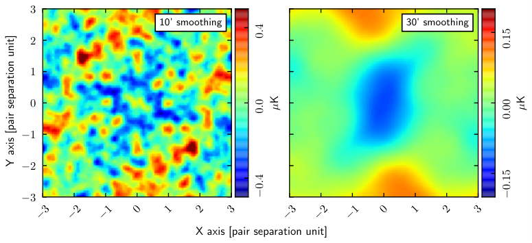
CO emission - In absence of any publicly available CO map, we take the Planck-derived MILCA 2015 CO () line emission map Planck_A1_2016 as a proxy for the CO emission. We choose Type 1 CO map as it has little contamination from other foregrounds, e.g. dust and emission. We smoothed the CO () Type 1 map at 10′ (FWHM) beam resolution taking into account the effective beam response of the Planck CO map and reduced to a HEALPix resolution of =1024. We then stack the CO map at the location of LRG pairs with K86 mask and the threshold . The left panel of Fig. 17 shows the stacked 10′ smoothed CO map at the location of LRG pairs. The stacked CO () map has no structure similar to the signal and is completely dominated by the CO noise. This also confirms our expectation using parameter fitting in section 4.2. To increase the signal-to-noise ratio, we choose to smoothed the CO () map to a beam resolution of 30′ FWHM. The stacking of 30′ smoothed CO () map is presented in the right panel of Fig. 17. The choice of 30′ smoothing scale is based on the power spectrum analysis of the CO map at high Galactic latitude Puglisi:2017. We take 30′ smoothed CO () map as a template for the CO emission (). We add CO contribution to 100 and 217 GHz channels only. For 217 GHz channel, we assume the line ratio of to as 0.595. The factor takes into account the spectrum of the CO emission at 100 and 217 GHz. For other frequencies, is set to zero.
- •
Instrumental noise - We add a random realization of simulated full focal plane (FFP8) noise map per frequency as an instrumental noise contribution Planck_A12_2016. It captures the dominant instrumental, scanning and map making algorithm and implementation noise effects.
We simulate all-sky simulated maps between 70 and 545 GHz at a common beam resolution of 10′ FWHM. These maps are expressed in units for frequencies between 70 and 353 GHz and MJy/sr for 545 GHz, similar to the real Planck data. Figure 18 compares the simulated maps over K86 mask with the real Planck data. We then perform the Stack First approach i.e. stacking the simulated frequency maps first at the LRG pair location over the threshold mask () with K86 mask and then perform the ILC on the stacked maps. Figure 19 shows the comparison between the simulated and the Planck stacked maps at frequencies between 70 and 545 GHz. The results and comparision with the stacked input map has been shown in the Figure 20. We find that the signal recovered using the Stack First approach indeed resembles the input signal obtained from the direct stacking of the LIL map. This confirms beyond doubt the capabilities of our approach in recovering faint signals by removing contaminations from the stacked frequency maps.
 |
| (a) |
 |
| (b) |
