Stability analysis and constraints on interacting viscous cosmology
Abstract
In this work we study the evolution of a spatially flat Universe by considering a viscous dark matter and perfect fluids for dark energy and radiation, including an interaction term between dark matter and dark energy. In the first part, we analyse the general properties of the Universe by performing a stability analysis and then we constrain the free parameters of the model using the latest and cosmological-independent measurements of the Hubble parameter. We find consistency between the viscosity coefficient and the condition imposed by the second law of the Thermodynamics. The second part is dedicated to constrain the free parameter of the interacting viscous model (IVM) for three particular cases: the viscous model (VM), interacting model (IM), and the perfect fluid case (the concordance model). We report the deceleration parameter to be , , , , together with the jerk parameter as , , , for the IVM, VM, IM, and LCDM respectively, where the uncertainties correspond at 68% CL. Worth mentioning that all the particular cases are in good agreement with LCDM, in some cases producing even better fits, with the advantage of eliminating some problems that afflicts the standard cosmological model.
Keywords:
dark energy, viscous fluids, interacting dark matter.I Introduction
Dark energy (DE) and dark matter (DM) are the corner stones of the modern cosmology, being so far one of the most intriguing mysteries for the understanding of our universe. In this vein, many attempts to comprehend the composition of this dark entities have been developed in recent years. The most important theories for DM are supersymmetry models (Martin:1997), scalar fields Magana:2012ph; Matos:1999et; Hernandez-Almada:2017mtm, interacting dark energy PhysRevD.99.043521; VONMARTTENS:2019; VONMARTTENS:2020, charged particles coming from unbroken gauge symmetry featuring dissipative interactions Vagnozzi:2015, among others, meanwhile for DE the most interesting candidates can be summarized as the cosmological constant (CC), phantom energy, quintessence, Chaplygin gas, brane-worlds, f(R), unimodular gravity etc. (see Refs. (Copeland:2006; Bamba:2012rev) for some reviews of DE models, also see Garcia-Aspeitia:2016kak; Garcia-Aspeitia:2018fvw; Hernandez-Almada:2018osh; Garcia-Aspeitia:2019yni; Astorga-Moreno:2019uin; Garcia-Aspeitia:2019yod). Despite the efforts of the community, the supersymetric DM and CC as dark energy are still the best candidates to understand the cosmological observations. However, laboratory experiments show no evidence of supersymmetric particles and the CC is afflicted with several theoretical problems (Weinberg; Zeldovich) when its origin is considered as quantum vacuum fluctuations. A radical new form to address these conflicts is to consider an interaction between the dark components through the continuity equation Chimento:2000; Copeland:2006; Bolotin:2015.
On the other hand, cosmology with viscous dark fluids is an interesting alternative to understand the accelerated expansion of the Universe Fabris:2006. The viscous fluid models could resolve the tension across different probes, for instance, the value of the Hubble constant () obtained from SNIa Anand:2017; Riess:2016 is more than the one estimated by CMB Planck data Planck:2016rXLVI, and the value of matter fluctuation amplitude () measured from the large scale structure (LSS) observations differs from those determined from the CMB Planck data under the LCDM cosmology DES:2018v26; DES:2018v28. Authors in Kremer:2012 study a dissipative Universe with interacting fluids which the non-equilibrium pressure is proportional to , they find that the decelerated - accelerated transition occurs earlier than the one of a non-viscous model (for other interesting models, see Avelino:2013; Atreya:2018; Valentino2019).
Although there are two types of viscosity coefficient known as bulk and shear, the bulk viscosity is the one that plays an important role in the Universe’s dynamics at the background level because it satisfies the cosmological principle. In contrast, one of the main characteristics of the shear viscosity is that it could produce vortices or any other chaotic phenomena at early epochs of the Universe evolution. Based on bulk viscosity, the viscous models have been addressed using two approaches: the Eckart Eckart:1940 and Israel-Stewart (IS) Israel1979 theories. For an extensive review on viscous cosmology, see Brevik:2017rev. The main difference between the theories is that the IS approach explored by Zimdahl:1996; Mak:1998; Paul:1998 solves the problem of the causality, i.e., the propagation of the perturbations on the viscous fluids is superluminal. Although this formalism avoids this problem is more complex than the Eckart theory, and only some analytical solutions MCruz:2017; NCruz:2018; NCruz:2018arx; NCruz:2019 are known for the bulk viscosity of the form , with and is the energy density of the viscous fluid in an Universe filled by only one fluid Burd:1988. In contrast, the Eckart’s scenario was the first proposal to study the relativistic dissipative processes as a first order deviations around the equilibrium and, despite the causality problem, it is widely used due to its simplicity. For instance, some works related to the Eckart’s theory, have been investigated the dynamics of the Universe at late times by considering a bulk viscous coefficient with a constant Murphy:1973; Padmanabhan:1987; Brevik2005; Normann:2017, polynomial Xin-He:2009; Avelino:2010; Almada:2019, and hyperbolic FOLOMEEV200875; Almada:2019 forms as functions of the redshift or in terms of the energy density. Additionally, authors in Normann:2016; Normann:2017 have been studied the Universe with several fluids, being a more realistic description of the Universe. In both theories, the procedure to include the bulk viscous effects into the Einstein field equations is trough as an effective pressure, written in the form , where refers to the sum of the traditional components such as the dust-matter (baryons, DM), the DE, and the relativistic species (photons, neutrinos), being an account to the bulk viscosity term. As a consequence, the equation of state (EoS) generally turns into an inhomogeneous one when the term is a variable function. Furthermore, it is worth noticing that letting , or any other dynamical variable, vary with time is an interesting way to explain the recent results given by Zhao:2017, which conclude a preference of the DE component for a dynamical EoS over a constant one. Regarding the physical mechanism to generate such viscous effects, some proposals point towards the decaying of DM particles Wilson:2007; Mathews:2008 or any other microscopic property as the self-interaction Atreya:2018 of DM particles.
Recently, the Experiment to Detect the Global EoR Signature (EDGES) Bowman:2018 found that the amplitude of the absorption signal of 21 cm temperature at the cosmic dawn epoch () is larger than expected. In this vein, the EDGES observations indicate that the baryons must be cooler or the photons hotter than the predicted by the standard cosmology, thus, this phenomenon offers another incentive to study the viscosity effects of the fluids and their interactions Barkana:2018; Bhatt:2019. Considering the first and second law of Thermodynamics and assuming the Universe filled by a non perfect DM fluid with , the authors in Bhatt:2019 find that the temperature of the DM fluid increase throughout the cosmic evolution due the bulk viscosity , thus, allow to describe the EDGES observations.
Therefore, in this work we study a model that consists of a flat Friedmann-Lemaıtre-Robertson-Walker (FLRW) Universe including three components: a non-perfect and interacting fluid, composed by DM where baryons are included, which we will call it as dust matter (dm) 11 1 Other models in literature separates the baryons from dark matter., the DE fluid that will interact with dm in the Eckart’s approach and radiation with its standard well known behavior. We start analyzing the general dynamics of these components through a stability analysis of the critical points. After that, we perform a Monte Carlo Chain Markov (MCMC) procedure using the latest observational Hubble parameter data (OHD) to constrain the free parameters of the model22 2 For instance, see Biswas:2005wy as another alternative to perform the dynamical system analysis in combination with Bayesian MCMC analysis.. Finally, we study particular cases of the model such as a solely viscous model (without the interaction term), an interacting model (without the viscosity term), and the perfect fluid case that correspond to the LCDM model.
The paper is organized as follow: In Sec. II presents the background of the interacting non-perfect model and gives the formulation of the dynamical system. In Sec. III we discuss the stability of the system around the critical points and give bounds to the free model parameters. Section IV is devoted to constrain the free parameters of the model using the latest samples of OHD. In Sec. V we discuss our results and finally, we present our remarks and conclusions in Sec.VI.
II Cosmology with Dark Fluids
The cosmological model under study consists of a Universe in a flat FLRW space time which contains a non-perfect fluid as dm that interacts with a perfect fluid as the DE component, together with the radiation fluid. Then, the energy-momentum tensor can be expressed as
| (1) |
where corresponds to the FLRW metric, is the sum of the total barotropic pressure of the fluids, , and the bulk viscosity coefficient, , is the energy density of the fluid and is the associated cuadri-velocity. Inspired on the viscosity behavior in fluid mechanics, being proportional to the speed, we have assumed . Additionally, the model supposes an energy exchange term between dm and DE, and a viscosity effect encoded in the terms that contain the bulk viscosity coefficient . In this approach, the Friedmann, continuity and acceleration equations are
| (2) | |||
| (3) | |||
| (4) | |||
| (5) | |||
| (6) |
where , , is the Newton gravitational constant, , , and correspond to the relativistic species, dust matter and dark energy densities respectively. The equation of state (EoS) for each species are , , and , being a constant that it is related with the EoS as . Notice that the DE component behaves as CC when .
In particular, in this work we consider the typical ansatz for the viscosity coefficient
| (7) |
where is the dm density at present epoch and is a free parameter with units of [eV].
To study the cosmological model presented in Eqs. (2)-(6), we define the dimensionless dynamical variables as
| (8) |
From Eq. (2), it is straightforward to see that . Then, the dynamical system can be written as Leyva:2017
| (9) | |||||
| (10) | |||||
where , and
| (11) |
In the latter equation notice that and are the fraction of dm and Hubble parameter at respectively. Additionally, to convert the dynamical system in an autonomous one we have defined the variable related to the interaction term. In particular, we will explore the form of as
| (12) |
or in terms of the dimensionless variables Zimdahl:2003
| (13) |
where is a dimensionless free parameter. It is evident that, for , the system described above corresponds to an Universe with viscosity. For alternative forms of that satisfy such conditions, see for instance Leyva:2017. In addition, we express the deceleration parameter, effective EoS and jerk parameter as Leyva:2017
| (14) | |||||
| (15) | |||||
| (16) |
where previous equations are written in terms of the dimensionless variables.
III Stability analysis
We start our stability study of the dynamical variables defined in the Eqs. (8)-(10) by finding the critical points and the Jacobian matrix, which are respectively
| (17) |
and
| (18) |
where
| (19) | |||||
| (20) | |||||
| (21) | |||||
| (22) | |||||
| Critical point | ( ) | Eigenvalues | Stability condition () |
|---|---|---|---|
| ( ) | Saddle if | ||
| ( ) | and | ||
| ( ) | Saddle |
The stability analysis of non linear systems consists in studying the behavior of the perturbations around the critical points using the matrix and decide if they are stable or not. Notice that for a vector that contains all the dynamical variables described in Eq. (8), we considered a small perturbation around the critical (or equilibrium) point , thus, an associated system is obtained in the form , where is the previously mentioned Jacobian matrix at the point . Hence, the Hartman-Grobman theorem guarantees that, for a critical point, there exists a neighborhood for which the flow of the system of dynamical equations is topologically equivalent to the linearized one Grobman; Hartman (see also Coley:2003; Leon:2014 for the dynamical system analysis in Cosmology). Hence, Table 1 summarizes the stability condition for each critical point. The first point, , represents the radiation dominant epoch with and . Notice that this point is a saddle for and unstable for . The latter condition guarantees the evolution of the Universe to another critical point that is expected to be .
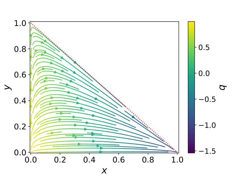
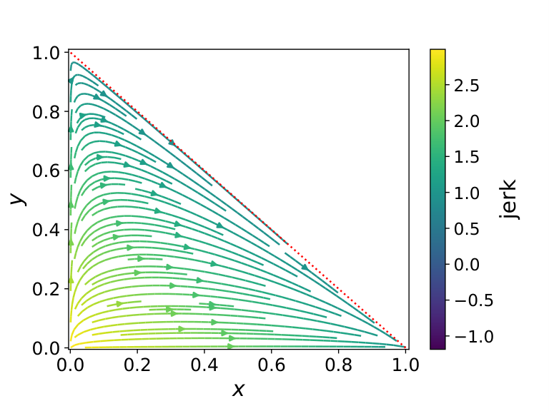
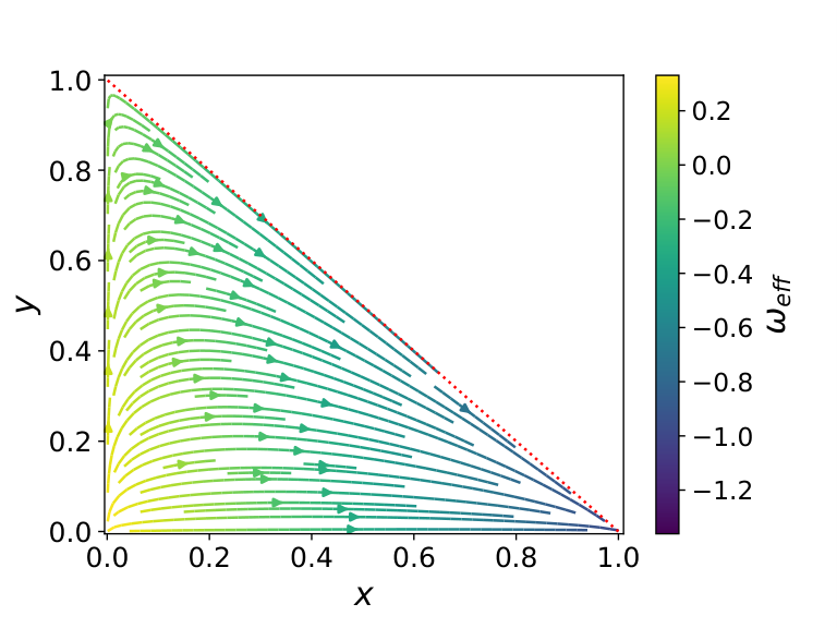
The point corresponds to the DM dominant epoch and it is stable in the region and . On the other hand, is a saddle point if and and an unstable point if and . Notice that the latter condition does not satisfy the second law of the thermodynamics that imposes Zimdahl:2000; Maartens:1996, and the saddle point gives a weaker condition for than the thermodynamic one. Moreover, structure formation is explained by the existence of in our dynamical system where the interaction term has no contribution. Furthermore, Figure 1 shows the {x,y}-phase space representing in gradient color the intensity of the deceleration (left panel) and jerk (middle panel) parameters and the effective EoS (right panel). In this phase-space, the evolution of the Universe starts around the point with , , and an effective EoS . Then, depending on the initial conditions of the Universe, it could change to a state close to with cosmographic parameters , , and . As mentioned before, this phase plays an important role in the structure formation, for that reason, an evolution with should not be allowed physically. The last stage of the Universe, where the accelerated expansion occurs, is when it moves towards the point with cosmographic parameters , , and .
IV Observational constraints
The expansion rate of the Universe is measured directly by the OHD. Currently, the OHD sample is obtained from the differential age technique and Baryon Acoustic Oscillations (BAO) measurements. In this work we consider the sample compiled by Magana:2018, that consists of points in the redshift region , to constrain the free model parameters. It is worth to note that this sample can yield biased constraints because the BAO points are estimated under a fiducial cosmology Magana:2018. Thus, the figure-of-merit is given by
| (23) |
where denotes the difference between the theoretical Hubble parameter with parameter space and the observational one at the redshift , and is the uncertainty of .
The data will be used not only to constrain our interacting viscous model (IVM) with free parameter space , but also the following particular models of the IVM: an only interacting model (IM) by setting , an only viscous model (VM) with , and the LCDM model that is recovered by requiring and . In order to solve the equation system, Eqs. (8)-(13), we have used for the initial condition of , and for , where , with as the number of relativistic species Komatsu:2011, and as the Hubble dimensionless parameter. To minimize the -function for each model, we perform a Bayesian MCMC analysis based on emcee module Emcee:2013. For each free model parameter, the n-burn phase is stopped following the Gelman-Rubin criteria Gelman:1992, i.e. after achieving a value lower than 1.1. We obtain chains, each one with steps, to explore the confidence region taking into account a Gaussian prior on the Hubble constant and a flat prior for the rest of the parameters (see Table 2).
| Parameter | Prior |
|---|---|
| Gauss | |
| Flat in | |
| Flat in | |
| Flat in |
Figure 2 displays our MCMC analysis for the free parameters with the 2D contours at (), (), and () confidence level (CL) and their corresponding 1D posterior distributions for IVM (green color), IM (red), VM (blue), and LCDM (grey) models. Table 3 shows the best fitting values for the free parameters and their uncertainties at () CL of the above mentioned cases. It is interesting to see that and are anti-correlated, which is an expected result because both parameters are acting to produce the accelerated expansion of the Universe. On the other hand, with the existence of a viscous Universe or an interacting dark sector (or both), we could establish a upper bound on the . We will discuss this bound in more detail in the next Section. Finally, Figure 3 displays the best fit curves over the OHD sample.
| Model | AIC | AIC | BIC | BIC | |||||
|---|---|---|---|---|---|---|---|---|---|
| IVM | |||||||||
| IM | |||||||||
| VM | |||||||||
| LCDM |
V Results and discussions
In this section we describe the physical properties of the Universe based on our results of the Bayesian MCMC analysis shown in Table 3. Figure 4 shows the evolution of the dynamical components , , and of the Universe described by IVM (top panel), and the evolution of the , , and parameters (bottom panel). It is important to remark that the behaves in concordance with standard cosmological model predictions (with Planck data, at Aghanim:2018). In other words, the Universe is in the quintessence region at late epochs (), as dust matter () around , and takes values closer to in the radiation phase (). In addition, the deceleration parameter is in the dm epoch, and increase towards in the radiation epoch. On the other hand, the jerk parameter is slightly below the value expected from LCDM () in the region going from the current epoch up to , and takes the expected value () for in the radiation dominated epoch. In summary, the presented models successfully reproduce all the expected epochs and are in good agreement with the LCDM model.
For a better statistical assessment of different models with different degrees of freedom we use, besides , the following criteria. The Akaike information criterion (AIC) AIC:1974; Sugiura:1978 and Bayesian Information criterion (BIC) schwarz1978 are defined as AIC and BIC respectively, where is the chi-squared function, is the number of degree of freedom and is the total number of data, being the model with the lowest value the one preferred by the data (see table III). If the difference in AIC value between a given model and the best one, AIC, is less than , both models are equally supported by the data. For the range AIC, the data still support the given model but less than the preferred one. For AIC, the observations do not support the given model. Thus, as it is shown in Table 3, when we compare the IM or VM with respect to LCDM (the preferred model), these models are equally preferred by the data (OHD+SNIa), being the IVM the least preferred by data. Similarly, the difference between a model and the best one, BIC, is interpreted as evidence against a candidate model being the best model. If BIC, there is no appreciable evidence against the model. In the range BIC, there is a modest evidence against the candidate model and if BIC, the evidence against the candidate model is strong; if BIC, the evidence against is even stronger. Thus, we have a strong evidence against IM and VM, and even stronger for IVM.
We estimate the deceleration-acceleration transition redshift takes place at , , , and for the IVM, VM, IM, and LCDM respectively, where the uncertainties correspond at CL. These values are consistent with those reported by Moresco:2016mzx of within . On the other hand, they are consistent with the one obtained by Kremer:2012 () when an interacting viscous model is considered. Additionally, our results are also compatible (within and respectively) with those found by Ref. Jesus:2019 using the non-parametric Gaussian Process method with the OHD data, ,and SNIa Pantheon sample, , and also the one value found by Haridasu:2018, when perform an extension of the standard Gaussian Process to Supernovae Type-Ia, BAO and Cosmic Chronometers data.
Regarding the cosmographic parameters, we obtain the deceleration one at to be , , , and for the IVM, VM, IM, and LCDM respectively. When we compare these results with the one obtained by Garcia-Aspeitia:2018fvw for the LCDM model, , we find a deviation within . Additionally, their corresponding value of the jerk parameter are , , , and . On the other hand, when we compare our and values with those obtained by Almada:2019 considering viscous models, we find a deviation of about . Additionally, we find a deviation on within for IVM, IV, and VM to the one value obtained in Haridasu:2018. Figure 5 shows 1D posterior distribution and 2D contours of the , , , and for IVM, IM, VM, and LCDM. Based on the IVM, it is noteworthy that presents a positive correlation () with and a negative one () with . The deceleration-acceleration transition has a negative correlation () with and a negligible correlation with . Between the cosmographic parameters (), we find a negative correlation of .

Figure 6 displays the 1D posterior distribution of the variables and for the IVM (green), IM (red), VM (blue), and LCDM (gray) together with the - contour at and CL. It is interesting to see that a possible effect of the interaction and viscosity terms is to increase the dm component at current epochs; nevertheless, such contributions are consistent within CL to the value of LCDM.
Only considering the DM component as the viscous one, the authors in Velten:2013 argue that, in the presence of several fluids in the Universe, it is difficult to distinguish which fluid is producing the viscous effects at the background level, in other words, there is degeneracy. However, as we mentioned in the introduction, when the DM fluid is the responsible for such dissipative effects it means that, at , the DM particles probably do not decay into energetic relativistic particles, such as sterile neutrinos or supersymmetric DM Wilson:2007. In this context, the DM particles should have a mass of the order and a lifetime of order the Hubble time . Based on the expression presented in Wilson:2007, where is the total energy density in the Universe, is the DM density for an unstable decaying DM, is the produced relativistic energy density, and is the equilibrium time with being the particle decaying time. Hence, we could give a bounded relation for such densities and the decaying lifetime at as at CL for the IVM and VM, respectively.
VI Conclusions and Outlooks
In this work we have addressed a phenomenological model for a flat Universe containing a radiation component and a viscous fluid (dark matter plus baryons) that interacts with a perfect fluid (DE), denoted as IVM. The IVM is characterized by the parameter phase-space . Furthermore, we studied some particular cases of the model by considering the dm fluid as an interacting perfect fluid (), and as only viscous fluid (). The latter consisted of the non-interacting perfect fluid () which corresponds to the LCDM model. In the first part of the work, we studied the IVM from a dynamical approach. We obtained the stability conditions for the critical points presented in the Table 1, which are in concordance with those obtained by Leyva:2017 when a linear interacting term of the form is considered, being an appropriate constant. Figure 1 shows the phase-space of the dynamical system where the color gradient represents the value of the deceleration parameter (), jerk (), and effective EoS (). The second part of the work consisted in performing a Bayesian MCMC analysis using the largest sample of the Hubble parameter data to obtain the best fit parameters for each model (Table 3). Then, we reconstructed the deceleration and jerk parameter and the effective EoS, as was shown in Fig. 4. We estimate the current values of the cosmographic parameters as , , , and , , , , for the IVM, VM, IM, and LCDM respectively, which are in agreement with those reported in the literature considering other models Garcia-Aspeitia:2018fvw; Almada:2019. Finally, although our results on BIC suggest the models used are unfavourable over LCDM standard paradigm, they give an alternative to alleviate the CC problems by adding some degree of freedom to LCDM.
Acknowledgments
We thank the anonymous referee for thoughtful remarks and suggestions. The authors acknowledge the enlightening conversation with Jesús Astorga. M.A.G.-A. acknowledges support from SNI-México, CONACyT research fellow, COZCyT and Instituto Avanzado de Cosmología (IAC) collaborations. J.M. acknowledges the support from CONICYT project Basal AFB-170002, V.M. acknowledges the support of Centro de Astrofísica de Valparaíso (CAV). J.M., M.A.G.-A. and V.M. acknowledge CONICYT REDES (190147).
References
- [1] Stephen P. Martin. A Supersymmetry primer. pages 1–98, 1997. [Adv. Ser. Direct. High Energy Phys.18,1(1998)].
- [2] Juan Magaña and Tonatiuh Matos. A brief Review of the Scalar Field Dark Matter model. J. Phys. Conf. Ser., 378:012012, 2012.
- [3] Tonatiuh Matos, Francisco Siddhartha Guzman, and L. Arturo Urena-Lopez. Scalar field as dark matter in the universe. Class. Quant. Grav., 17:1707–1712, 2000.
- [4] A. Hernández-Almada and Miguel A. García-Aspeitia. Multistate scalar field dark matter and its correlation with galactic properties. Int. J. Mod. Phys., D27(03):1850031, 2017.
- [5] Rodrigo von Marttens, Valerio Marra, Luciano Casarini, J. E. Gonzalez, and Jailson Alcaniz. Null test for interactions in the dark sector. Phys. Rev. D, 99:043521, Feb 2019.
- [6] R. von Marttens, L. Casarini, D.F. Mota, and W. Zimdahl. Cosmological constraints on parametrized interacting dark energy. Physics of the Dark Universe, 23:100248, 2019.
- [7] Rodrigo von Marttens, Lucas Lombriser, Martin Kunz, Valerio Marra, Luciano Casarini, and Jailson Alcaniz. Dark degeneracy i: Dynamical or interacting dark energy? Physics of the Dark Universe, 28:100490, 2020.
- [8] R. Foot and S. Vagnozzi. Dissipative hidden sector dark matter. Phys. Rev. D, 91:023512, Jan 2015.
- [9] E. J. Copeland, M. Sami, and S. Tsujikawa. Dynamics of dark energy. International Journal of Modern Physics D, 15(11):1753–1935, 2006.
- [10] Kazuharu Bamba, Salvatore Capozziello, Shin’ichi Nojiri, and Sergei D. Odintsov. Dark energy cosmology: the equivalent description via different theoretical models and cosmography tests. Astrophysics and Space Science, 342(1):155–228, Nov 2012.
- [11] Miguel A. García-Aspeitia, Juan Magaña, Alberto Hernández-Almada, and V. Motta. Probing dark energy with braneworld cosmology in the light of recent cosmological data. IJMPD, 27:18560006, 2018.
- [12] Miguel A. García-Aspeitia, A. Hernández-Almada, Juan Magaña, Mario H. Amante, V. Motta, and C. Martínez-Robles. Brane with variable tension as a possible solution to the problem of the late cosmic acceleration. Phys. Rev., D97(10):101301, 2018.
- [13] Hernández-Almada, A., Magaña, Juan, García-Aspeitia, Miguel A., and Motta, V. Cosmological constraints on alternative model to chaplygin fluid revisited. Eur. Phys. J. C, 79(1):12, 2019.
- [14] Miguel A. García-Aspeitia, C. Martínez-Robles, A. Hernández-Almada, Juan Magaña, and V. Motta. Cosmic acceleration in unimodular gravity. Phys. Rev., D99(12):123525, 2019.
- [15] J. A. Astorga-Moreno, Javier Chagoya, J. C. Flores-Urbina, and Miguel A. García-Aspeitia. Compact objects in unimodular gravity. JCAP, 1909:005, 2019.
- [16] Miguel A. García-Aspeitia, A. Hernández-Almada, Juan Magaña, and V. Motta. On the birth of the cosmological constant and the reionization era. 2019.
- [17] Steven Weinberg. The cosmological constant problem. Reviews of Modern Physics, 61, 1989.
- [18] Ya. B. Zeldovich. The cosmological constant and the theory of elementary particles. Soviet Physics Uspekhi, 11, 1968.
- [19] Luis P. Chimento, Alejandro S. Jakubi, and Diego Pavón. Enlarged quintessence cosmology. Phys. Rev. D, 62:063508, Aug 2000.
- [20] Yuri L. Bolotin, Alexander Kostenko, Oleg A. Lemets, and Danylo A. Yerokhin. Cosmological evolution with interaction between dark energy and dark matter. International Journal of Modern Physics D, 24(03):1530007, 2015.
- [21] J. C. Fabris, S. V. B. Gonçalves, and R. de Sá Ribeiro. Bulk viscosity driving the acceleration of the universe. General Relativity and Gravitation, 38(3):495–506, Mar 2006.
- [22] Sampurn Anand, Prakrut Chaubal, Arindam Mazumdar, and Subhendra Mohanty. Cosmic viscosity as a remedy for tension between PLANCK and LSS data. Journal of Cosmology and Astroparticle Physics, 2017(11):005–005, nov 2017.
- [23] Adam G. Riess, Lucas M. Macri, Samantha L. Hoffmann, Dan Scolnic, Stefano Casertano, Alexei V. Filippenko, Brad E. Tucker, Mark J. Reid, David O. Jones, Jeffrey M. Silverman, Ryan Chornock, Peter Challis, Wenlong Yuan, Peter J. Brown, and Ryan J. Foley. A 2.4% determination of the local value of the Hubble constant. The Astrophysical Journal, 826(1):56, jul 2016.
- [24] Planck Collaboration, Aghanim, N., and et. al. Planck intermediate results - XLVI. reduction of large-scale systematic effects in HFI polarization maps and estimation of the reionization optical depth. A&A, 596:A107, 2016.
- [25] T. M. C. Abbott and et. al. Dark energy survey year 1 results: Cosmological constraints from galaxy clustering and weak lensing. Phys. Rev. D, 98:043526, Aug 2018.
- [26] M. A. Troxel and et. al. Dark energy survey year 1 results: Cosmological constraints from cosmic shear. Phys. Rev. D, 98:043528, Aug 2018.
- [27] Gilberto M. Kremer and Octavio A. S. Sobreiro. Bulk viscous cosmological model with interacting dark fluids. Brazilian Journal of Physics, 42(1):77–83, Apr 2012.
- [28] Arturo Avelino, Yoelsy Leyva, and L. Arturo Ureña López. Interacting viscous dark fluids. Phys. Rev. D, 88:123004, Dec 2013.
- [29] Abhishek Atreya, Jitesh R. Bhatt, and Arvind Mishra. Viscous self interacting dark matter and cosmic acceleration. Journal of Cosmology and Astroparticle Physics, 2018(02):024–024, feb 2018.
- [30] Eleonora Di Valentino, Alessandro Melchiorri, Olga Mena, and Sunny Vagnozzi. Interacting dark energy after the latest planck, des, and measurements: an excellent solution to the and cosmic shear tensions. 2019.
- [31] Carl Eckart. The thermodynamics of irreversible processes. iii. relativistic theory of the simple fluid. Phys. Rev., 58:919–924, Nov 1940.
- [32] W. Israel and J.M. Stewart. Transient relativistic thermodynamics and kinetic theory. Annals of Physics, 118(2):341 – 372, 1979.
- [33] Iver Brevik, Øyvind Grøn, Jaume de Haro, Sergei D. Odintsov, and Emmanuel N. Saridakis. Viscous cosmology for early- and late-time universe. International Journal of Modern Physics D, 26(14):1730024, 2017.
- [34] Winfried Zimdahl. Bulk viscous cosmology. Phys. Rev. D, 53:5483–5493, May 1996.
- [35] M. K. Mak. Exact causal viscous cosmologies. Gen. Rel. Grav., 30:1171–1186, 1998.
- [36] B. C. Paul, S. Mukherjee, and A. Beesham. Higher derivative theory with viscosity. International Journal of Modern Physics D, 07(04):499–507, 1998.
- [37] Miguel Cruz, Norman Cruz, and Samuel Lepe. Accelerated and decelerated expansion in a causal dissipative cosmology. Phys. Rev. D, 96:124020, Dec 2017.
- [38] Norman Cruz, Esteban González, Samuel Lepe, and Diego Sáez-Chillón Gómez. Analysing dissipative effects in the CDM model. Journal of Cosmology and Astroparticle Physics, 2018(12):017–017, dec 2018.
- [39] Guillermo Palma Norman Cruz, Esteban González. Exact solutions for a cosmology within the Israel-Stewart theory. 2018.
- [40] Norman Cruz, A. Hernández-Almada, and Octavio Cornejo-Pérez. Constraining a causal dissipative cosmological model. Phys. Rev. D, 100:083524, Oct 2019.
- [41] A.B. Burd and John D. Barrow. Inflationary models with exponential potentials. Nuclear Physics B, 308(4):929 – 945, 1988.
- [42] George L. Murphy. Big-bang model without singularities. Phys. Rev. D, 8:4231–4233, Dec 1973.
- [43] T. Padmanabhan and S.M. Chitre. Viscous universes. Physics Letters A, 120(9):433 – 436, 1987.
- [44] I. Brevik and O. Gorbunova. Dark energy and viscous cosmology. General Relativity and Gravitation, 37(12):2039–2045, Dec 2005.
- [45] Ben David Normann and Iver Brevik. Characteristic properties of two different viscous cosmology models for the future universe. Modern Physics Letters A, 32(04):1750026, 2017.
- [46] Meng Xin-He and Dou Xu. Friedmann cosmology with bulk viscosity: A concrete model for dark energy. Communications in Theoretical Physics, 52(2):377, 2009.
- [47] Arturo Avelino and Ulises Nucamendi. Exploring a matter-dominated model with bulk viscosity to drive the accelerated expansion of the universe. Journal of Cosmology and Astroparticle Physics, 2010(08):009–009, aug 2010.
- [48] A. Hernández-Almada. Cosmological test on viscous bulk models using hubble parameter measurements and type ia supernovae data. The European Physical Journal C, 79(9):751, Sep 2019.
- [49] Vladimir Folomeev and Victor Gurovich. Viscous dark fluid. Physics Letters B, 661(2):75 – 77, 2008.
- [50] Ben David Normann and Iver Brevik. General bulk-viscous solutions and estimates of bulk viscosity in the cosmic fluid. Entropy, 18(6), 2016.
- [51] Gong-Bo Zhao, Marco Raveri, and et. al. Dynamical dark energy in light of the latest observations. Nature Astronomy, 1:627–632, 2017.
- [52] James R. Wilson, Grant J. Mathews, and George M. Fuller. Bulk viscosity, decaying dark matter, and the cosmic acceleration. Phys. Rev. D, 75:043521, Feb 2007.
- [53] G. J. Mathews, N. Q. Lan, and C. Kolda. Late decaying dark matter, bulk viscosity, and the cosmic acceleration. Phys. Rev. D, 78:043525, Aug 2008.
- [54] R. A. Monsalve T. J. Mozdzen J. D. Bowman, A. E. E. Rogers and N. Mahesh. An absorption profile centred at 78 megahertz in the sky-averaged spectrum. Nature, 555(7694):67, 2018.
- [55] R. Barkana. Possible interaction between baryons and dark-matter particles revealed by the first stars. Nature, 555:71–74, March 2018.
- [56] Jitesh R. Bhatt, Arvind Kumar Mishra, and Alekha C. Nayak. Viscous dark matter and 21 cm cosmology. Phys. Rev. D, 100:063539, Sep 2019.
- [57] Tirthabir Biswas, Robert Brandenberger, Anupam Mazumdar, and Tuomas Multamaki. Current acceleration from dilaton and stringy cold dark matter. Phys. Rev., D74:063501, 2006.
- [58] Yoelsy Leyva and Mirko Sepúlveda. Bulk viscosity, interaction and the viability of phantom solutions. The European Physical Journal C, 77(6):426, Jun 2017.
- [59] Winfried Zimdahl and Diego Pavón. Scaling cosmology. General Relativity and Gravitation, 35(3):413–422, Mar 2003.
- [60] D. Grobman. Homeomorphisms of systems of differential equations. Dokl. Akad.,Nauk., 128:880–881, 1959.
- [61] P. Hartman. A lemma in the theory of structural stability of differential equations. Proc.Amer. Math. Soc.,, 11:610–620, 1960.
- [62] A. A. Coley. Dynamical Systems and Cosmology, volume 291. 2003.
- [63] Genly Leon and Carlos R. Fadragas. Cosmological dynamical systems. LAP Lambert Academic Publishing, 2012.
- [64] Winfried Zimdahl and Diego Pavón. Expanding universe with positive bulk viscous pressures? Phys. Rev. D, 61:108301, Apr 2000.
- [65] Roy Maartens. Causal thermodynamics in relativity, 1996.
- [66] Juan Magaña, Mario H Amante, Miguel A García-Aspeitia, and V Motta. The cardassian expansion revisited: constraints from updated hubble parameter measurements and type ia supernova data. Monthly Notices of the Royal Astronomical Society, 476(1):1036–1049, 2018.
- [67] E. Komatsu and et. al. The Astrophysical Journal Supplement Series, 192(2):18, jan 2011.
- [68] D. Foreman-Mackey, D. W. Hogg, D. Lang, and J. Goodman. emcee: The MCMC Hammer. pasp, 125:306, March 2013.
- [69] A. Gelman and D.B. Rubin. Inference from iterative simulation using multiple sequences. Statistical Science, 67:457–511, 1992.
- [70] N. Aghanim et al. Planck 2018 results. VI. Cosmological parameters. 2018.
- [71] H. Akaike. A new look at the statistical model identification. IEEE Transactions on Automatic Control, 19(6):716–723, December 1974.
- [72] Nariaki Sugiura. Further analysts of the data by akaike’s information criterion and the finite corrections. Communications in Statistics - Theory and Methods, 7(1):13–26, 1978.
- [73] Gideon Schwarz. Estimating the dimension of a model. Ann. Statist., 6(2):461–464, 03 1978.
- [74] Michele Moresco, Lucia Pozzetti, Andrea Cimatti, Raul Jimenez, Claudia Maraston, Licia Verde, Daniel Thomas, Annalisa Citro, Rita Tojeiro, and David Wilkinson. A 6% measurement of the Hubble parameter at : direct evidence of the epoch of cosmic re-acceleration. JCAP, 1605(05):014, 2016.
- [75] J. F. Jesus, R. Valentim, A. A. Escobal, and S. H. Pereira. Gaussian process estimation of transition redshift, 2019.
- [76] Balakrishna S. Haridasu, Vladimir V. Luković, Michele Moresco, and Nicola Vittorio. An improved model-independent assessment of the late-time cosmic expansion. Journal of Cosmology and Astroparticle Physics, 2018(10):015–015, oct 2018.
- [77] Hermano Velten, Jiaxin Wang, and Xinhe Meng. Phantom dark energy as an effect of bulk viscosity. Phys. Rev. D, 88:123504, Dec 2013.