Supermassive Neutron Stars in Axion GravitySupermassive Neutron Stars in Axion Gravity–References
Abstract
We investigated realistic neutron stars in axion gravity. The coupling between curvature and axion field is assumed in the simple form . For the axion mass in the range eV the solitonic core within neutron star and corresponding halo with size km can exist. Therefore the effective contribution of term grows inside the star and it leads to change of star parameters (namely, mass and radius). We obtained the increase of star mass independent from central density for wide range of masses. Therefore, maximal possible mass for given equation of state grows. At the same time, the star radius increases not so considerably in comparison with GR. Hence, our model may predict possible existence of supermassive compact stars with masses and radii km for realistic equation of state (we considered APR equation of state). In General Relativity one can obtain neutron stars with such characteristics only for unrealistic, extremely stiff equations of state. Note that this increase of mass occurs due to change of solution for scalar curvature outside the star. In GR curvature drops to zero on star surface where . In the model under consideration the scalar curvature dumps more slowly in comparison with vacuum gravity due to axion “galo” around the star.
Keywords:
neutron stars – modified gravity – axions1 Introduction
There are still unresolved fundamental puzzles in modern cosmology and relativistic astrophysics. One of them is so-called dark energy which governs the observed accelerated universe expansion (Riess, et al. 1998; Perlmutter, et al. 1999; Riess, et al. 2004). According to the well-known CDM model, dark energy is simply Cosmological Constant and its density is 72% of the global energy budget of the universe. The remaining 28%, clustered in galaxies and clusters of galaxies, consist of baryons (only 4%) and cold dark matter (CDM) the nature of which is unclear. Alternative approach to description of late-time cosmological dynamics of universe is proposed by theories of modified gravity (Capozziello & Fang 2002; Nojiri & Odintsov 2003; Carroll, et al. 2004).
Furthermore, the unified description of observed late-time acceleration and early universe expansion is also possible in the context of theory (Nojiri & Odintsov 2003). Matter and radiation dominance eras can be also described in frames of this approach (for review, see refs. Nojiri & Odintsov 2011; Capozziello & de Laurentis 2011; Olmo 2011; de la Cruz-Dombriz & Sáez-Gómez 2012; Nojiri, Odintsov & Oikonomou 2017).
Another problem of current cosmology and high energy physics is dark matter. There are many evidences in favor for particle nature of dark matter (for example, see data about collision of galaxies in the Bullet Cluster and cluster MACSJ0025 (Markevitch, et al. 2003; Clowe, et al. 2006; Robertson, Massey & Eke 2017; Bradač, et al. 2008)). As the candidates on the role of dark matter the weakly interacted massive particles (WIMPs) have been considered usually. Many approaches to direct observation of such particles were proposed but so far the direct experiments for detection of such particles have not been successful ( see CDMS II Collaboration, et al. 2010; Davis, McCabe & Bœhm 2014; Davis 2015; Roszkowski, Sessolo & Trojanowski 2018; Schumann 2019).
Another possibility is that dark matter is nothing else than axions (Sakharov & Khlopov 1994; Sakharov, Sokoloff & Khlopov 1996; Khlopov, Sakharov & Sokoloff 1999; Marsh 2016; Marsh, et al. 2017; Odintsov & Oikonomou 2019; Cicoli, Guidetti & Pedro 2019; Fukunaga, Kitajima & Urakawa 2019; Caputo 2019). Some recent experiments indicate in favor for its existence (Du, et al. 2018; Henning, et al. 2018; Ouellet, et al. 2019; Safdi, Sun & Chen 2019; Avignone, Creswick & Vergados 2018; Caputo, et al. 2019; Caputo, Garay & Witte 2018; Lawson, et al. 2019; Rozner, et al. 2019). Mass of axions can be very low (theoretical estimations give value in the wide range eV). The possibility of axions detection is based on axion-photon interaction in the presence of magnetic fields (Balakin & Ni 2010; Balakin, Bochkarev & Tarasova 2012; Balakin, Muharlyamov & Zayats 2014).
Recently, axion F(R) gravity was discussed in ref. Odintsov & Oikonomou 2019 in which the unification of dark energy with axion dark matter (and eventually, with inflation) was proposed. For the description of axion in this model misalignment model was used (Anisimov & Dine 2005). According to misagliment model the primordial U(1) Peccei-Quinn symmetry is broken during inflation. For it was chosen simple model and non-minimal coupling with axion field in the form .
It is interesting to address the question about possible manifestations of modified gravity with various scalar fields (including axions) on astrophysical level. First of all, one should pay attention to relativistic stars for which the energy density in the center is around g/cm3 and therefore gravitational field is extremely high. In principle, for such strong gravity regime the possible deviations from General Relativity can be visible somehow. Unfortunately we have no well established data about mass-radius diagram for neutron stars from astronomical observations. Mass, radius and other parameters of relativistic stars also depend from the equation of state chosen for dense matter. There is now clear understanding how nuclear matter behaves at such extremely densities and tens of EoS were proposed over the years (for some introduction, see ref. Rezzolla, et al. 2018).
This paper is devoted to the study of neutron stars in frames of gravity coupled with axion field in the form where is some constant. It is interesting to note that Compton wavelength for particle with mass eV is km. This scale is comparable with characteristic size of neutron stars. Therefore one can consider the possibility of existence of solitonic core containing dark matter in the center of the star. The contribution to energy density from such core is negligible itself and therefore couldn’t influence on the parameters of star. However, the assumption of coupling can lead to non-trivial deviations from General Relativity.
gravity was considered as viable alternative to GR for description of stellar structure in some papers. The question of hydrostatic equilibrium was studied in ref. Capozziello, et al. 2011. Dynamics and collapse of collisionless self-gravitating systems in gravity was firstly investigated by Capozziello, et al. 2012. It is interesting to note also iterative procedure for the solution of modified Lane-Emden equation considered in Farinelli, et al. 2014. For neutron stars initially the perturbative approach was used. The scalar curvature is defined by Einstein equations at zeroth order on the small parameter, i.e. , where is the trace of energy-momentum tensor. This approach is applied to construction of neutron star models in and gravity also in Arapoǧlu, Deliduman & Eksi 2011, Alavirad & Weller 2013; Astashenok, Capozziello & Odintsov 2013.
In modified gravity model with cubic and quadratic terms, it is possible to obtain neutron stars with for simple hyperon equations of state (EoS) although the soft hyperon equation of state is usually treated as non-realistic in the standard General Relativity (Astashenok, Capozziello & Odintsov 2014). The possible signatures of modified gravity in neutron star astrophysics also can include existence of neutron stars with extremely high magnetic fields (Cheoun, et al. 2013; Astashenok, Capozziello & Odintsov 2015). Interesting results were obtained for gravity in Capozziello, et al. 2016. Detailed analysis of neutron stars structure in gravity was given by authors in ref. Astashenok, Odintsov & de la Cruz-Dombriz 2017. It is shown that so-called gravitational sphere with nonzero curvature appears around the star. Recently the mass-radius relation in both metric and torsional gravity were investigated in Feola, et al. 2019. For recent review of compact star models in modified theories of gravity see Olmo, Rubiera-Garcia & Wojnar 2019 and references therein.
The main problem of simple gravity is that possible observable consequences appear only if the contribution of -term is sufficiently large. The motivation for the consideration of non-minimal coupling in the form is that axion field can strengthen the contribution of -term only inside star due to solitonic core. Outside the star the scalar field and scalar curvature quickly drop in fact to zero value (of course, in comparison with corresponding values inside the star).
In the next section we start from the equations for stellar configurations in gravity in quasi-isotropic coordinates. For their derivation the so-called formalism is used. as a result we get the system of equations of elliptical type for unknown metric functions and scalar curvature . The account of scalar field requires one more equation. The results of the calculation including mass profile, mass-radius diagram, scalar curvature and axion field are given in the section III. For neutron star matter the well-known APR EoS is used. Our calculations show that qualitative behavior of solutions doesn’t depend from chosen EoS.
2 3+1 formalism in f(R) gravity
We start from the well-known Einstein equations in frames of General Relativity
| (1) |
Here is the Ricci tensor associated with the Levi-Civita connection in 4-dimensional spacetime, is the scalar curvature and is the energy-momentum tensor of matter. The system of units in which is used.
Firstly we consider simple gravity with the action
| (2) |
from which it follows that Einstein equations are
| (3) |
Here is covariant D’Alamber operator and . Then we drop arguments of .
For the study of compact stars in general relativity the 3+1 formalism is often used (Gourgoulhon 2010; Alcubierre 2008; Baumgarte & Shapiro 2010; Gourgoulhon 2007). One can adopt this method for gravity without any significant changes.
The key moment is foliation of spacetime by spacelike hypersurfaces . Parameter can be associated with coordinate time. The next step is the definition of metric induced by metric on hypersurface . The components of induced metric can be given via the components of unit timelike normal vector n and metric :
| (5) |
We also define the components of orthogonal projector onto hypersurface by raising of the first index:
| (6) |
We use metric of special form
| (7) |
where is so-called lapse function and is shift vector. The 3-dimensional metric is the metric induced on surface. Then projecting the Einstein equation (4) twice onto , (ii) twice along to vector normal to and (iii) once on and once along , one gets the following three equations:
| (8) |
| (9) |
| (10) |
where is tensor of extrinsic curvature and . One also introduces the components of Lie derivative of tensor and along the vector :
| (11) |
The covariant derivatives can be expressed in terms of partial derivatives with respect to the spatial coordinates by means of the Christoffel symbols of associated with :
| (12) |
| (13) |
| (14) |
For 3-dimensional Ricci tensor and scalar curvature we have following relations:
| (15) |
| (16) |
The quantities , and are energy density, components of stress tensor and vector of energy flux density correspondingly. These values can be obtained from stress-energy tensor :
| (17) |
Then we take the trace of first equation:
| (18) |
From equation (9) it follows that
and therefore one can rewrite the previous equation as
| (19) |
Let us consider the non-rotating stellar configurations. In this case all metric functions depend only from radial coordinate. For convenience we used isotropic spatial coordinates with metric in the form
| (20) |
For this metric one can obtain that
We also have the following expression for 3-dimensional scalar curvature:
Taking into account that
one can rewrite the equation for in the following form
| (21) |
In this relation is nothing else than radial part of -dimensional Laplace operator in Euclidean space.
The energy-momentum tensor in the case of spherical symmetry can be presented in diagonal form where is pressure of matter and therefore
The action of 3-dimensional covariant D’Alamber operator for any scalar function depending only from radial coordinate is reduced to
| (22) |
For 4-dimensional d’Alambertian one obtains the simple relation:
| (23) |
Finally Eq. (19) for our task can be presented in the form:
| (24) |
Here and . Let us consider eq. (9) for metric (20). Using relations for and covariant d’Alambertian one gets
| (25) |
Next, one considers the -component of (8). One need to use the following representations for and :
One obtains after simple calculations
| (26) |
| (28) |
In General Relativity scalar curvature is simply and therefore it approaches to zero on the surface of star where . For gravity one needs additional equation for scalar curvature. This equation can be obtained from trace of Einstein equations and for our case of radial dependence of scalar curvature it takes the form:
| (29) |
For the case of function depending also from scalar field these equations are valid. For radial derivatives of function one should remember that
Assuming the action for axion field in the following form
| (30) |
one can obtain the equation for scalar field :
| (31) |
The system of equations (24), (27), (29), (31) should be supplemented by a set of boundary conditions for , , and . Those are provided by the asymptotic flatness assumption. On spatial infinity the metric tensor tends towards Minkowski metric and therefore
For scalar field we also assume that when because the density of dark matter in the space ( g/cm3) is extremely low in comparison with densities inside relativistic stars.
Asymptotical behavior of at defines gravitational mass of star for distant observer. In General Relativity the solution of Einstein equations outside the star has the form:
| (32) |
Therefore, the gravitational mass of star can be found as an asymptotical limit
One should also account that physical radial coordinate is
Note that in the following the symbol “r” on figures means physical distance. Tildes are omitted for simplicity.


| , MeV/fm3 | , | , | , km | , | |
|---|---|---|---|---|---|
| GR | 1.64 | 11.25 | 0.0674 | - | |
| 0 | 1.68 | 11.40 | 0.0674 | - | |
| 650 | 100 | 1.65 | 11.38 | 0.0273 | 0.0097 |
| 250 | 1.67 | 11.42 | 0.0183 | 0.0094 | |
| 1000 | 1.73 | 11.48 | 0.0077 | 0.0076 | |
| GR | 1.92 | 11.03 | 0.0146 | - | |
| 0 | 1.98 | 11.15 | 0.0137 | - | |
| 800 | 100 | 2.00 | 11.26 | 0.0238 | 0.0097 |
| 250 | 2.04 | 11.33 | 0.0162 | 0.0096 | |
| 1000 | 2.12 | 11.44 | 0.0071 | 0.0077 | |
| GR | 2.10 | 10.68 | -0.0889 | - | |
| 0 | 2.14 | 10.80 | -0.0899 | - | |
| 1000 | 100 | 2.19 | 10.89 | 0.0142 | 0.0077 |
| 250 | 2.22 | 10.95 | 0.0108 | 0.0080 | |
| 1000 | 2.30 | 11.07 | 0.0051 | 0.0068 |
3 Results
We considered in detail the model with the action
| (33) |
Following to Marsh 2016 we consider only small deviations from the potential minimum. Therefore, the leading term is
The behavior of axion scalar is mainly governed by term. Another key moment of this model is the influence of scalar field on the dependence of scalar curvature from radial coordinate.
For axion mass we take the value corresponding to Compton wavelength where is gravitational radius of Sun ( km). For the parameter the range in units of is explored.
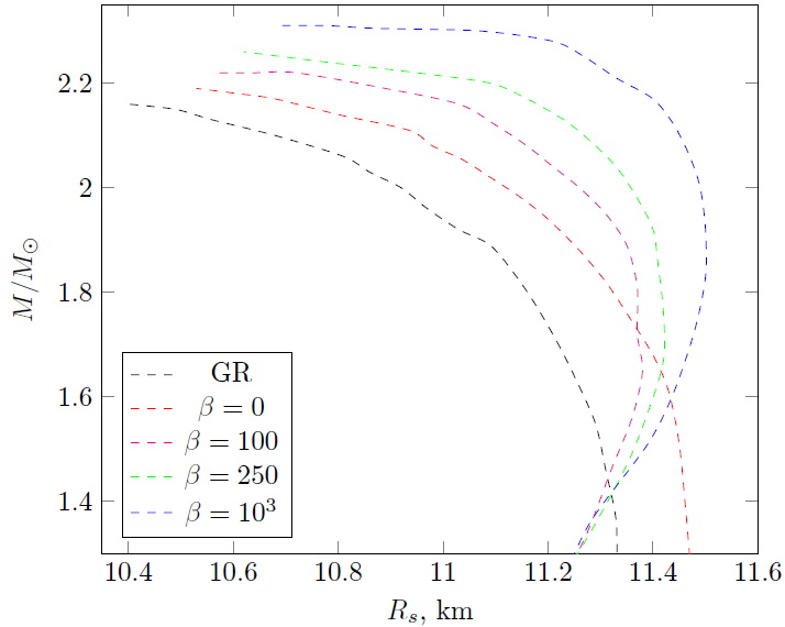
First of all, let us consider the case when the parameter is relatively small (for example ). The mass-radius diagram can be seen on Fig. 1 with the dependence of stellar mass from the energy density in the center of star. For massive stars one can see (Table I) that increase of mass for consists of or % (in comparison with General Relativity) for the same density in the center of star. The radius of star also increases and therefore for given radius the increase of mass looks even bigger. Therefore one can expect that in such modified gravity the fraction of supermassive neutron stars (with ) should increase. Another interesting point is the maximal possible mass for given equation of state. For APR equation we have that 2.31 at in comparison with ) in General Relativity. Note that mass increases with nonlinearly and for very large this increase does not exceed significantly the result obtained for . In General Relativity one can obtain compact stars with and km only for very stiff equations of state usually treated as unrealistic.
It is interesting to consider the mass profile for various parameters of model. On Fig. 2 the for three values of (650, 800 and 1000 MeV/fm3) is depicted. The increase of gravitational mass of star for distant observer occurs due to non-trivial behavior of scalar curvature outside the star (Fig. 3). For GR outside the star and for simple -model of gravity scalar curvature decreases quickly outside the star. Due to axion field (see Fig. 4) the damping of scalar curvature became smoother.
The increase of parameter in considered area () does not lead to significant consequences for stellar masses. For example on Fig. 5 the radial profiles of scalar curvature, axion field and mass are depicted for fixed value of and two values of : and . One can see that increase of leads to some decrease of axion field and curvature (therefore contribution of term decreases). Note that we don’t consider the case of very large () by the following reason. One can see that value of curvature within star is . Therefore term for will be larger in comparison with . Therefore from physical viewpoint such values of seems unrealistic.
One can also mention about the influence of axion mass on the solution of gravitational equations. We considered (corresponding to Compton wavelength and found that in this case only solution of scalar field outside the star changes considerably (see Fig. 6) but scalar curvature for km is very close to zero and therefore contribution of term is negligible.
We also considered in our preliminary calculations the potential with term but in this case deviations from simple model are very negligible.
4 Conclusion
We investigated neutron stars in axion gravity with non-minimal curvature-axion coupling in form . Our main result is possible increase of stellar mass due to axion presence. We obtained the increase of mass for massive stars in the case of . This value is sufficient for possible observational indication of such model. The star radius increases not so considerably ( m for ). Therefore, axion gravity under consideration may explain the possible existence of supermassive neutron stars () compact as in general relativity at the same time. There are some indications in favor of the existence of such neutron stars (for example the possible masses of B1957+20 (van Kerkwijk, Breton & Kulkarni 2011) and 4U 1700-377 (Clark, et al. 2002) are ).
Axion field affects on behavior of scalar curvature inside and outside star in comparison with General Relativity and vacuum gravity. Increase of mass for distant observer occurs due to “gravitational sphere” outside the star with nonzero curvature. The star radius increases and mass confined inside the stellar surface decreases in comparison with General Relativity but the contribution of gravitational sphere overcompensates this decrease. In contrast to simple square gravity increase of gravitational mass is relatively equal for various values of density in the center of star up to the masses close to maximum. Therefore, the increase of maximal mass takes place. For instance, we obtained that in the case of APR equation of state maximal mass is 2.31 instead of 2.15 in General Relativity for some choice of parameters. Increase of radius also take place but it is not so significant and hardly observable.
Our calculations show also interesting effect of some “compensation” between two terms, i.e. and . If increases the contribution of second term decreases due to damping mean value of curvature and axion field. As the consequence we have no possibility to discriminate between various solutions corresponding to various parameters.
Characteristic scale of curvature damping in pure gravity is . We considered the case when this value is smaller in comparison with Compton wavelength of axion field (). For very large Compton wavelength (, for example) we have no observable consequences on masses and radii of stellar configurations. Only radius of axion “galo” around the star grows.
Although, for illustration we used the star models based on well-known APR equation of state our calculations lead to qualitatively similar results for other realistic choices of equation of state for dense matter in neutron stars. Finally, one can expect that combined effect of axion dark matter and modified gravity maybe quite significant in stellar astrophysics at strong gravitational regime.
One should mention recent paper (Riley, et al. 2019) in which authors found promising mass-radius posteriors for mass and radius of pulsar PSR J0030+0451. We think that these results on current stage can exclude some equations of state for which radius of star with mass differs significantly from narrow range. In the light of these data APR equation of state is under question in General Relativity and as consequence in our model because for possible value of radius differs from GR value negligibly (this difference is m for model with axions and this value is less in comparison with error of measurements (1 km)). For equation of state describing these data the picture is the same. In this case if GR fits these data well then our theory does the same.
One can ask how would one differentiate between considered model of simple gravity with axions and simply for example the case with different equation of state for dense matter? Eventually, the observational indication towards our model may soon appear if the expected experiments may confirm that axion is indeed the dark matter. From another side, R2 gravity gives the best realistic candidate for inflation. Again, if future more precise Planck/BICEP data will confirm axion R2 inflation that will be the best proof of viability of current model for supermassive neutron stars.
Acknoweledgments. This work is partly supported by MINECO (Spain), FIS2016-76363-P, by COST Action PHAROS (CA16214), by project 2017 SGR247 (AGAUR, Catalonia) (SDO). AVA thanks the Program 5-100 (IKBFU, Russia).
References
- CDMS II Collaboration, et al. (2010) CDMS II Collaboration, et al., 2010, Sci, 327, 1619
- Alavirad & Weller (2013) Alavirad H., Weller J. M., 2013, PhRvD, 88, 124034
- Alcubierre (2008) Alcubierre M., 2008, itnr.book
- Arapoǧlu, Deliduman & Eksi (2011) Arapoǧlu S., Deliduman C., Eksi K. Y., 2011, JCAP, 2011, 020
- Astashenok, Capozziello & Odintsov (2013) Astashenok A. V., Capozziello S., Odintsov S. D., 2013, JCAP, 2013, 040
- Astashenok, Capozziello & Odintsov (2014) Astashenok A. V., Capozziello S., Odintsov S. D., 2014, PhRvD, 89, 103509
- Astashenok, Capozziello & Odintsov (2015) Astashenok A. V., Capozziello S., Odintsov S. D., 2015, Ap&SS, 355, 333
- Astashenok, Odintsov & de la Cruz-Dombriz (2017) Astashenok A. V., Odintsov S. D., de la Cruz-Dombriz Á., 2017, CQGra, 34, 205008
- Avignone, Creswick & Vergados (2018) Avignone F. T., Creswick R. J., Vergados J. D., 2018, arXiv, arXiv:1801.02072
- Balakin & Ni (2010) Balakin A. B., Ni W.-T., 2010, CQGra, 27, 055003
- Balakin, Bochkarev & Tarasova (2012) Balakin A. B., Bochkarev V. V., Tarasova N. O., 2012, EPJC, 72, 1895
- Balakin, Muharlyamov & Zayats (2014) Balakin A. B., Muharlyamov R. K., Zayats A. E., 2014, EPJD, 68, 159
- Baumgarte & Shapiro (2010) Baumgarte T. W., Shapiro S. L., 2010, nure.book
- Bradač, et al. (2008) Bradač M., et al., 2008, ApJ, 687, 959
- Capozziello & Fang (2002) Capozziello S., Fang L. Z., 2002, IJMPD, 11, 483
- Capozziello & de Laurentis (2011) Capozziello S., de Laurentis M., 2011, PhR, 509, 167
- Capozziello, et al. (2011) Capozziello S., de Laurentis M., Odintsov S. D., Stabile A., 2011, PhRvD, 83, 064004
- Capozziello, et al. (2012) Capozziello S., de Laurentis M., de Martino I., Formisano M., Odintsov S. D., 2012, PhRvD, 85, 044022
- Capozziello, et al. (2016) Capozziello S., De Laurentis M., Farinelli R., Odintsov S. D., 2016, PhRvD, 93, 023501
- Caputo, et al. (2019) Caputo A., Regis M., Taoso M., Witte S. J., 2019, JCAP, 2019, 027
- Caputo, Garay & Witte (2018) Caputo A., Garay C. P., Witte S. J., 2018, PhRvD, 98, 083024
- Caputo (2019) Caputo A., 2019, PhLB, 797, 134824
- Carroll, et al. (2004) Carroll S. M., Duvvuri V., Trodden M., Turner M. S., 2004, PhRvD, 70, 043528
- Cheoun, et al. (2013) Cheoun M.-K., Deliduman C., Güngör C., Keles V., Ryu C. Y., Kajino T., Mathews G. J., 2013, JCAP, 2013, 021
- Cicoli, Guidetti & Pedro (2019) Cicoli M., Guidetti V., Pedro F. G., 2019, JCAP, 2019, 046
- Clark, et al. (2002) Clark J. S., Goodwin S. P., Crowther P. A., Kaper L., Fairbairn M., Langer N., Brocksopp C., 2002, A&A, 392, 909
- Clowe, et al. (2006) Clowe D., Bradač M., Gonzalez A. H., Markevitch M., Randall S. W., Jones C., Zaritsky D., 2006, ApJL, 648, L109
- de la Cruz-Dombriz & Sáez-Gómez (2012) de la Cruz-Dombriz A., Sáez-Gómez D., 2012, Entrp, 14, 1717
- Davis, McCabe & Bœhm (2014) Davis J. H., McCabe C., Bœhm C., 2014, JCAP, 2014, 014
- Davis (2015) Davis J. H., 2015, IJMPA, 30, 1530038
- Anisimov & Dine (2005) Anisimov A., Dine M., 2005, JCAP, 2005, 009
- Du, et al. (2018) Du N., et al., 2018, PhRvL, 120, 151301
- Farinelli, et al. (2014) Farinelli R., De Laurentis M., Capozziello S., Odintsov S. D., 2014, MNRAS, 440, 2909
- Feola, et al. (2019) Feola P., Jimenez Forteza X., Capozziello S., Cianci R., Vignolo S., 2019, arXiv, arXiv:1909.08847
- Fukunaga, Kitajima & Urakawa (2019) Fukunaga H., Kitajima N., Urakawa Y., 2019, JCAP, 2019, 055
- Gourgoulhon (2007) Gourgoulhon E., 2007, arXiv, gr-qc/0703035
- Gourgoulhon (2010) Gourgoulhon E., 2010, arXiv, arXiv:1003.5015
- Henning, et al. (2018) [ABRACADABRA Collaboration], 2018, DOI: 10.3204/DESY-PROC-2017-02/henning_reyco
- van Kerkwijk, Breton & Kulkarni (2011) van Kerkwijk M. H., Breton R. P., Kulkarni S. R., 2011, ApJ, 728, 95
- Khlopov, Sakharov & Sokoloff (1999) Khlopov M. Y., Sakharov A. S., Sokoloff D. D., 1999, NuPhS, 72, 105
- Lawson, et al. (2019) Lawson M., Millar A. J., Pancaldi M., Vitagliano E., Wilczek F., 2019, PhRvL, 123, 141802
- Markevitch, et al. (2003) Markevitch M., et al., 2003, ApJ, 583, 70
- Marsh (2016) Marsh D. J. E., 2016, PhR, 643, 1
- Marsh, et al. (2017) Marsh M. C. D., Russell H. R., Fabian A. C., McNamara B. R., Nulsen P., Reynolds C. S., 2017, JCAP, 2017, 036
- Nojiri & Odintsov (2003) Nojiri S., Odintsov S. D., 2003, PhRvD, 68, 123512
- Nojiri & Odintsov (2003) Nojiri S., Odintsov S. D., 2003, PhLB, 576, 5
- Nojiri, Odintsov & Oikonomou (2017) Nojiri S., Odintsov S. D., Oikonomou V. K., 2017, PhR, 692, 1
- Nojiri & Odintsov (2011) Nojiri S., Odintsov S. D., 2011, PhR, 505, 59
- Odintsov & Oikonomou (2019) Odintsov S. D., Oikonomou V. K., 2019, PhRvD, 99, 104070
- Odintsov & Oikonomou (2019) Odintsov S. D., Oikonomou V. K., 2019, PhRvD, 99, 104070
- Olmo (2011) Olmo G. J., 2011, IJMPD, 20, 413
- Olmo, Rubiera-Garcia & Wojnar (2019) Olmo G. J., Rubiera-Garcia D., Wojnar A., 2019, arXiv, arXiv:1912.05202
- Perlmutter, et al. (1999) Perlmutter S., et al., 1999, ApJ, 517, 565
- Ouellet, et al. (2019) Ouellet J. L., et al., 2019, PhRvL, 122, 121802
- Rezzolla, et al. (2018) Rezzolla L., Pizzochero P., Jones D. I., Rea N., Vidaña I., 2018, ASSL..457
- Riess, et al. (1998) Riess A. G., et al., 1998, AJ, 116, 1009
- Riess, et al. (2004) Riess A. G., et al., 2004, ApJ, 607, 665
- Riley, et al. (2019) Riley T. E., et al., 2019, ApJL, 887, L21
- Robertson, Massey & Eke (2017) Robertson A., Massey R., Eke V., 2017, MNRAS, 465, 569
- Roszkowski, Sessolo & Trojanowski (2018) Roszkowski L., Sessolo E. M., Trojanowski S., 2018, RPPh, 81, 066201
- Rozner, et al. (2019) Rozner M., Grishin E., Ginat Y. B., Igoshev A. P., Desjacques V., 2019, arXiv, arXiv:1904.01958
- Safdi, Sun & Chen (2019) Safdi B. R., Sun Z., Chen A. Y., 2019, PhRvD, 99, 123021
- Sakharov & Khlopov (1994) Sakharov A. S., Khlopov M. Y., 1994, PAN, 57, 651
- Sakharov, Sokoloff & Khlopov (1996) Sakharov A. S., Sokoloff D. D., Khlopov M. Y., 1996, PAN, 59, 1005
- Schumann (2019) Schumann M., 2019, JPhG, 46, 103003