跳到论文正文
W Papers独立论文阅读器 arXiv:2001.08459 论文正文 计算阅读时间 · 0%
引用这篇论文根据当前论文元数据生成,正式投稿前建议核对。


License: arXiv.org perpetual non-exclusive license
arXiv:2001.08459v2 [hep-ph] 02 Sep 2020

Study of semileptonic decay of B¯s0→ϕ​l+​l−\bar{B}_{s}^{0}\to\phi l^{+}l^{-} in QCD sum rule

Ying-Quan Peng Email: 2120170119@mail.nankai.edu.cn Affiliation: School of Physics, Nankai University,Tianjin 300071, People’s Republic of China    Mao-Zhi Yang Email: yangmz@nankai.edu.cn Affiliation: School of Physics, Nankai University,Tianjin 300071, People’s Republic of China
Abstract

In this work we study the semi-leptonic decay of B¯s0→ϕ​l+​l−\bar{B}_{s}^{0}\to\phi l^{+}l^{-} (l=e,μ,τl=e,\mu,\tau) with QCD sum rule method. We calculate the B¯s0→ϕ\bar{B}_{s}^{0}\to\phi translation form factors relevant to this semi-leptonic decay, then the branching ratios of B¯s0→ϕ​l+​l−\bar{B}_{s}^{0}\to\phi l^{+}l^{-} (l=e,μ,τl=e,\mu,\tau) decays are calculated with the form factors obtained here. Our result for the branching ratio of B¯s0→ϕ​μ+​μ−\bar{B}_{s}^{0}\to\phi\mu^{+}\mu^{-} agrees very well with the recent experimental data. For the unmeasured decay modes such as B¯s0→ϕ​e+​e−\bar{B}_{s}^{0}\to\phi e^{+}e^{-} and B¯s0→ϕ​τ+​τ−\bar{B}_{s}^{0}\to\phi\tau^{+}\tau^{-}, we give theoretical predictions.

Keywords: 
Semileptonic decay, form factor, QCD sum rule
pacs
13.20.He,11.55.Hx,12.15.Lk

I Introduction

In the Standard Model, flavor-changing neutral current (FCNC) induced processes are forbidden at tree level. They can only occur via loop diagrams. Meanwhile they are also sensitive to contributions of new physics. Particles of new physics may contribute via loop diagrams as “virtual particles”, thereby affecting the physical processes induced by FCNC. With continuous improvement of experimental accuracy, FCNC processes play an increasingly important role in the new physics research in heavy flavour physics. The most typical process is the one caused by b→s​l+​l−b\to sl^{+}l^{-}, such as the rare semi-leptonic decays of B¯s0→ϕ​l+​l−\bar{B}_{s}^{0}\to\phi l^{+}l^{-} (l=e,μ,τl=e,\mu,\tau).

In the past two decades, the decays of B¯s0→ϕ​l+​l−\bar{B}_{s}^{0}\to\phi l^{+}l^{-} (l=e,μ,τl=e,\mu,\tau) have been studied by using several different approaches such as lattice QCD (LQCD) LQCD, QCD light-cone sum rule (LCSR) LCSR; LCSR-improve, constituent quark model (CQM) CQM-G; CQM-Me, QCD sum rule R.K-SumR, relativistic quark model (RQM) FG and covariant quark model CoQM. The method of QCD sum rule (SR) was originally developed by Shifman, Vainshtein and Zakharov in the late 1970s SVZ1; SVZ2, which was then widely applied to the calculation of hadronic physics Colan2000. Several years ago the translation form factors of B¯s0→ϕ\bar{B}^{0}_{s}\to\phi in B¯s0→ϕ​l+​l−\bar{B}_{s}^{0}\to\phi l^{+}l^{-} (l=e,μ,τl=e,\mu,\tau) decays were calculated with QCD sum rule in Ref. R.K-SumR. Compared with other results, some form factors obtained in Ref. R.K-SumR are different by negative signs, which are not simply due to different definition for the form factors.

Experimentally, LHCb Collaboration updated the measurement of the branching ratio of B¯s0→ϕ​μ+​μ−\bar{B}_{s}^{0}\to\phi\mu^{+}\mu^{-} recently 15AQ ,

Br​(B¯s0→ϕ​μ+​μ−)=(7.97−0.43+0.45±0.22±0.23±0.60)×10−7.\mbox{Br}(\bar{B}_{s}^{0}\to\phi\mu^{+}\mu^{-})=(7.97^{+0.45}_{-0.43}\pm 0.22\pm 0.23\pm 0.60)\times 10^{-7}. (1)

Hence, considering the status of theoretical calculation and the recent improvement in experimental measurement, we believe that it is valuable to re-consider the decays of B¯s0→ϕ​l+​l−\bar{B}_{s}^{0}\to\phi l^{+}l^{-} (l=e,μ,τl=e,\mu,\tau) theoretically. In this work, we revisit the form factors in B¯s0→ϕ\bar{B}_{s}^{0}\to\phi transition in QCD sum rule, and use these form factors to calculate the branching ratios of B¯s0→ϕ​e+​e−\bar{B}_{s}^{0}\to\phi e^{+}e^{-}, B¯s0→ϕ​μ+​μ−\bar{B}_{s}^{0}\to\phi\mu^{+}\mu^{-} and B¯s0→ϕ​τ+​τ−\bar{B}_{s}^{0}\to\phi\tau^{+}\tau^{-}. Finally, we compare our results of form factors and branching ratios with previous theoretical works as well as the latest experimental data.

The paper is organized as followings. In Sec. II, we present the effective Hamiltonian and effective amplitude of B¯s0→ϕ​l+​l−\bar{B}_{s}^{0}\to\phi l^{+}l^{-} decay. Section III ∼\thicksim IV are devoted to the calculation of the form factors in QCD sum rule method. Section V is for the numerical analysis and discussion. Finally, a brief summary is presented in Sec. VI.

II Effective Hamiltonian

At quark level, the effective Hamiltonian of the rare semileptonic decay b→s​l+​l−b\to sl^{+}l^{-} can be written as hamiltonian,

ℋeff=−GF2Vt​bVt​s∗∑i=110Ci(μ)Oi(μ),\mathcal{H}_{{\rm eff}}=-\frac{G_{F}}{\sqrt{2}}V_{tb}V_{ts}^{*}\sum_{i=1}^{10}{C_{i}(\mu)O_{i}(\mu)}, (2)

where Vt​b​Vt​s∗V_{tb}V_{ts}^{*} is the product of relevant CKM matrix elements. CiC_{i} denotes Wilson coefficient, and the operators OiO_{i} are

Q1=(s¯α​cβ)V−A​(c¯β​bα)V−A,\displaystyle Q_{1}=(\bar{s}_{\alpha}c_{\beta})_{V-A}(\bar{c}_{\beta}b_{\alpha})_{V-A}, Q2\displaystyle Q_{2} =(s¯​c)V−A​(c¯​b)V−A,\displaystyle=(\bar{s}c)_{V-A}(\bar{c}b)_{V-A},
Q3=(s¯​b)V−A​∑q(q¯​q)V−A,\displaystyle Q_{3}=(\bar{s}b)_{V-A}\sum_{q}(\bar{q}q)_{V-A}, Q4\displaystyle Q_{4} =(s¯α​bβ)V−A​∑q(q¯β​qα)V−A,\displaystyle=(\bar{s}_{\alpha}b_{\beta})_{V-A}\sum_{q}(\bar{q}_{\beta}q_{\alpha})_{V-A},
Q5=(s¯​b)V−A​∑q(q¯​q)V+A,\displaystyle Q_{5}=(\bar{s}b)_{V-A}\sum_{q}(\bar{q}q)_{V+A}, Q6\displaystyle Q_{6} =(s¯α​bβ)V−A​∑q(q¯β​qα)V+A,\displaystyle=(\bar{s}_{\alpha}b_{\beta})_{V-A}\sum_{q}(\bar{q}_{\beta}q_{\alpha})_{V+A},
Q7=αe2​π​mb​s¯α​σμ​ν​(1+γ5)​bα​Fμ​ν,\displaystyle Q_{7}=\frac{\alpha_{e}}{2\pi}m_{b}\bar{s}_{\alpha}\sigma^{\mu\nu}(1+\gamma^{5})b_{\alpha}F_{\mu\nu}, Q8\displaystyle Q_{8} =αs2​π​mb​s¯α​σμ​ν​(1+γ5)​Tα​βa​bβ​Gμ​νa,\displaystyle=\frac{\alpha_{s}}{2\pi}m_{b}\bar{s}_{\alpha}\sigma^{\mu\nu}(1+\gamma^{5})T_{\alpha\beta}^{a}b_{\beta}G_{\mu\nu}^{a},
Q9=α2​π​(s¯​b)V−A​(l¯​l)V,\displaystyle Q_{9}=\frac{\alpha}{2\pi}(\bar{s}b)_{V-A}(\bar{l}l)_{V}, Q10\displaystyle~Q_{10} =α2​π​(s¯​b)V−A​(l¯​l)A.\displaystyle=\frac{\alpha}{2\pi}(\bar{s}b)_{V-A}(\bar{l}l)_{A}.

Then the effective Hamiltonian above leads to the following decay amplitude of B¯s0→ϕ​l+​l−\bar{B}_{s}^{0}\to\phi l^{+}l^{-} hamiltonian

ℳ⁡(B¯s0→ϕ​l+​l−)\displaystyle\mathcal{M}(\bar{B}_{s}^{0}\to\phi l^{+}l^{-}) =\displaystyle= GF​α2​2​πVt​bVt​s∗[C9eff⟨ϕ(ε,p2)|s¯γν(1−γ5)b|B¯s0(p1)⟩ℓ¯γνℓ\displaystyle\frac{G_{F}\alpha}{2\sqrt{2}\pi}V_{tb}V_{ts}^{*}\left[C^{{\rm eff}}_{9}\langle\phi(\varepsilon,p_{2})|\bar{s}\gamma_{\nu}(1-\gamma_{5})b|\bar{B}_{s}^{0}(p_{1})\rangle\bar{\ell}\gamma^{\nu}\ell\right. (3)
+C10​⟨ϕ⁡(ε,p2)​|s¯​γν​(1−γ5)​b|​B¯s0​(p1)⟩​ℓ¯​γν​γ5​ℓ\displaystyle\left.+C_{10}\langle\phi(\varepsilon,p_{2})|\bar{s}\gamma_{\nu}(1-\gamma_{5})b|\bar{B}_{s}^{0}(p_{1})\rangle\bar{\ell}\gamma^{\nu}\gamma_{5}\ell\right.
−2C7effmbiq2⟨ϕ(ε,p2)|s¯σν​λqλ(1+γ5)b|B¯s0(p1)⟩ℓ¯γνℓ]\displaystyle\left.-2C^{{\rm eff}}_{7}m_{b}\frac{{\rm i}}{q^{2}}\langle\phi(\varepsilon,p_{2})|\bar{s}\sigma_{\nu\lambda}q^{\lambda}(1+\gamma_{5})b|\bar{B}_{s}^{0}(p_{1})\rangle\bar{\ell}\gamma^{\nu}\ell\right]

where p1p_{1} and p2p_{2} are momenta of B¯s0\bar{B}_{s}^{0} and ϕ\phi mesons, respectively. qq is the momentum transfer q=p1−p2q=p_{1}-p_{2}. C9effC^{{\rm eff}}_{9} and C7effC^{{\rm eff}}_{7} are two effective Wilson coefficients, with C7eff=C7−C5/3−C6C^{{\rm eff}}_{7}=C_{7}-{C_{5}}/3-C_{6}. As for the effective Wilson coefficient C9effC^{{\rm eff}}_{9}, we take the expression in Ref. hamiltonian, which is given as followings

C9eff\displaystyle C^{{\rm eff}}_{9} =\displaystyle= C9+C0​[h⁡(m^c,s^)+3​π​κα2​∑Vi=ψ⁡(1​s,2​s)Γ⁡(Vi→l+​l−)​mVimVi2−q2−i​mVi​ΓVi]\displaystyle C_{9}+C_{0}\left[h(\hat{m}_{c},\hat{s})+\frac{3\pi\kappa}{\alpha^{2}}\sum_{V_{i}=\psi(1s;2s)}\frac{\Gamma(V_{i}\to l^{+}l^{-})m_{V_{i}}}{m^{2}_{V_{i}}-q^{2}-{\rm i}m_{V_{i}}\Gamma_{V_{i}}}\right] (4)
−\displaystyle- 12​h​(1,s^)​(4​C3+4​C4+3​C5+C6)\displaystyle\frac{1}{2}h(1,\hat{s})(4C_{3}+4C_{4}+3C_{5}+C_{6})
−\displaystyle- 12​h​(0,s^)​(C3+3​C4)+29​(3​C3+C4+3​C5+C6),\displaystyle\frac{1}{2}h(0,\hat{s})(C_{3}+3C_{4})+\frac{2}{9}(3C_{3}+C_{4}+3C_{5}+C_{6}),

where we define

C0=3​C1+C2+3​C3+C4+3​C5+C6,C_{0}=3C_{1}+C_{2}+3C_{3}+C_{4}+3C_{5}+C_{6},
h⁡(0,s^)=827−89​ln⁡mbμ−49​ln⁡s^+i​π​49,h(0,\hat{s})=\frac{8}{27}-\frac{8}{9}\ln{\frac{m_{b}}{\mu}}-\frac{4}{9}\ln{\hat{s}}+{\rm i}\pi\frac{4}{9},

and

h⁡(m^c,s^)=−89​ln⁡mbμ−89​ln⁡m^c+827+49​x−29​(2+x)​|1−x|12​{(ln⁡|1−x+11−x−1|−i​π),x<12​arctan⁡1x−1,x>1,h(\hat{m}_{c},\hat{s})=-\frac{8}{9}\ln{\frac{m_{b}}{\mu}}-\frac{8}{9}\ln{\hat{m}_{c}}+\frac{8}{27}+\frac{4}{9}x-\frac{2}{9}(2+x)|1-x|^{\frac{1}{2}}\left\{\begin{array}[]{rcl}&&(\ln{|\frac{\sqrt{1-x}+1}{\sqrt{1-x}-1}|-{\rm i}\pi}),~{x<1}\\ &&2\arctan{\frac{1}{\sqrt{x-1}}}~~~~~,~{x>1}\end{array}\right.,

with x=4​m^c2/s^x={4{\hat{m}}_{c}}^{2}/{\hat{s}}, m^c=mc/mBs\hat{m}_{c}={m_{c}}/{m_{B_{s}}}, s^=q2/mBs2\hat{s}={q^{2}}/{m^{2}_{B_{s}}}, κ=1/C0\kappa={1}/{C_{0}} and μ=mb\mu=m_{b}.

III Form Factors from QCD Sum Rule

We have calculated the hadronic matrix elements ⟨ϕ⁡(ε,p2)​|s¯​γν​(1−γ5)​b|​B¯s0​(p1)⟩\langle\phi(\varepsilon,p_{2})|\bar{s}\gamma_{\nu}(1-\gamma_{5})b|\bar{B}_{s}^{0}(p_{1})\rangle in the decay amplitude given in Eq. (3) in our previous work PYQ. So in this work, we need only to deal with the other hadronic matrix element ⟨ϕ⁡(ε,p2)​|s¯​σν​λ​qλ​(1+γ5)​b|​B¯s0​(p1)⟩\langle\phi(\varepsilon,p_{2})|\bar{s}\sigma_{\nu\lambda}q^{\lambda}(1+\gamma_{5})b|\bar{B}_{s}^{0}(p_{1})\rangle in Eq. (3).

Similarly the hadronic matrix element ⟨ϕ|s¯​σν​λ​qλ​(1+γ5)​b|B¯s0⟩\langle\phi|\bar{s}\sigma_{\nu\lambda}q^{\lambda}(1+\gamma_{5})b|\bar{B}_{s}^{0}\rangle can be decomposed as Lu/form-factors

⟨ϕ⁡(ε,p2)​|s¯​σν​λ​qλ​(1+γ5)​b|​B¯s0​(p1)⟩\displaystyle\langle\phi(\varepsilon,p_{2})|\bar{s}\sigma_{\nu\lambda}q^{\lambda}(1+\gamma_{5})b|\bar{B}_{s}^{0}(p_{1})\rangle =\displaystyle= 2​i​εν​ρ​α​β​ε∗ρ​p1α​p2β​T1​(q2)\displaystyle 2{\rm i}\varepsilon_{\nu\rho\alpha\beta}\varepsilon^{*\rho}p_{1}^{\alpha}p_{2}^{\beta}T_{1}(q^{2}) (5)
+[εν∗​(mBs2−mϕ2)−(ε∗⋅q)​(p1+p2)ν]​T2​(q2)\displaystyle+[\varepsilon^{*}_{\nu}(m_{B_{s}}^{2}-m_{\phi}^{2})-(\varepsilon^{*}\cdot q)(p_{1}+p_{2})_{\nu}]T_{2}(q^{2})
+(ε∗⋅q)​[qν−q2mBs2−mϕ2​(p1+p2)ν]​T3​(q2),\displaystyle+(\varepsilon^{*}\cdot q)[q_{\nu}-\frac{q^{2}}{m_{B_{s}}^{2}-m_{\phi}^{2}}(p_{1}+p_{2})_{\nu}]T_{3}(q^{2}),

where T1T_{1}, T2T_{2} and T3T_{3} are the transition form factors associated with the current of jνT​(0)=s¯​σν​λ​qλ​(1+γ5)​bj^{T}_{\nu}(0)=\bar{s}\sigma_{\nu\lambda}q^{\lambda}(1+\gamma_{5})b.

As what we did in Ref. PYQ, at first we consider a three-point correlation function that is defined as

Πμ​ν=i2​∫d4​x​d4​y​ei​p2⋅x−i​p1⋅y​⟨0|T⁡{jμϕ​(x)​jνT​(0)​j5​(y)}|0⟩,\Pi_{\mu\nu}={\rm i}^{2}\int{\rm d}^{4}x{\rm d}^{4}y{\rm e}^{{\rm i}p_{2}\cdot x-{\rm i}p_{1}\cdot y}\langle 0|T\{j^{\phi}_{\mu}(x)j^{T}_{\nu}(0)j_{5}(y)\}|0\rangle, (6)

where jμϕ​(x)=s¯​(x)​γμ​s​(x)j_{\mu}^{\phi}(x)=\bar{s}(x)\gamma_{\mu}s(x), jνT​(0)=s¯​σν​λ​qλ​(1+γ5)​bj^{T}_{\nu}(0)=\bar{s}\sigma_{\nu\lambda}q^{\lambda}(1+\gamma_{5})b and j5​(y)=b¯​(y)​i​γ5​s​(y)j_{5}(y)=\bar{b}(y){\rm i}\gamma_{5}s(y), which are the current of ϕ\phi channel, the current of weak transition and the current of B¯s0\bar{B}_{s}^{0} channel, respectively.

Next we reexpress the correlation function by using the double dispersion relation

Πμ​ν=∫d​s1​d​s2​ρ⁡(s1,s2,q2)(s1−p12)​(s2−p22),\Pi_{\mu\nu}=\int{\rm d}s_{1}{\rm d}s_{2}\frac{\rho(s_{1},s_{2},q^{2})}{(s_{1}-p_{1}^{2})(s_{2}-p_{2}^{2})}, (7)

where the spectral density function ρ⁡(s1,s2,q2)\rho(s_{1},s_{2},q^{2}) can be expressed as the form containing a full set of intermediate hadronic states as shown below,

ρ⁡(s1,s2,q2)=∑X∑Y⟨0|jμϕ​|X⟩​⟨X|jνT|Y⟩​⟨Y|​j5|0⟩​δ​(s1−mY2)​δ​(s2−mX2)​θ​(pX0)​θ​(pY0),\rho(s_{1},s_{2},q^{2})=\sum_{X}\sum_{Y}\langle 0|j_{\mu}^{\phi}|X\rangle\langle X|j^{T}_{\nu}|Y\rangle\langle Y|j_{5}|0\rangle\delta(s_{1}-m_{Y}^{2})\delta(s_{2}-m_{X}^{2})\theta(p_{X}^{0})\theta(p_{Y}^{0}), (8)

where XX and YY denote the full set of hadronic states of ϕ\phi and B¯s0\bar{B}^{0}_{s} channels, respectively. According to Eqs. (7) and (8), we can integrate over s1s_{1} and s2s_{2}, then separate the ground states, excited states and continuum states, the correlation function can be expressed as

Πμ​ν=mϕ​fϕ​εμ(λ)​⟨ϕ⁡(εμ(λ),p2)​|jνT|​B¯s0​(p1)⟩​fBs​mBs2(mBs2−p12)​(mϕ2−p22)​(mb+ms)\displaystyle\Pi_{\mu\nu}=\frac{m_{\phi}f_{\phi}\varepsilon_{\mu}^{(\lambda)}\langle\phi(\varepsilon_{\mu}^{(\lambda)},p_{2})|j^{T}_{\nu}|\bar{B}_{s}^{0}(p_{1})\rangle f_{B_{s}}m_{B_{s}}^{2}}{(m_{B_{s}}^{2}-p_{1}^{2})(m_{\phi}^{2}-p_{2}^{2})(m_{b}+m_{s})}
+excited and continuum states.\displaystyle+\mbox{\small{excited and continuum states}}. (9)

In the above equation, we have used the following definition of relevant matrix elements

⟨0|s¯​γμ​s|ϕ⟩=mϕ​fϕ​εμ(λ),\displaystyle\langle 0|\bar{s}\gamma_{\mu}s|\phi\rangle=m_{\phi}f_{\phi}\varepsilon_{\mu}^{(\lambda)},
⟨0|s¯​i​γ5​b|B¯s0⟩=fBs​mBs2mb+ms,\displaystyle\langle 0|\bar{s}{\rm i}\gamma_{5}b|\bar{B}_{s}^{0}\rangle=\frac{f_{B_{s}}m_{B_{s}}^{2}}{m_{b}+m_{s}}, (10)

where fϕf_{\phi} and fBsf_{B_{s}} are decay constants of the relevant mesons. In principle, ϕ\phi and ω\omega can mix via strong interaction, the mixing angle δ\delta between nonstrange and strange quark wave function has been analyzed to be δ=−(3.34±0.17)∘\delta=-(3.34\pm 0.17)^{\circ} Benayoun1; Kucu; Gronau1; Benayoun2; Gronau2, which shows that ϕ\phi meson is dominated by component s​s¯s\bar{s}. Therefore, we can safely drop the mixing effect of ω−ϕ\omega-\phi in Ds→ϕD_{s}\to\phi transition process, and ϕ\phi meson is treated as s​s¯s\bar{s} component, which is referred to as ideal mixing.

By taking the operator product expansion (OPE) for the time-ordered current operator in Eq. (6), we can get another expression for the correlation function in terms of Wilson coefficients and condensates of local operators

Πμ​ν\displaystyle\Pi_{\mu\nu} =\displaystyle= i2​∫d4​x​d4​y​ei​p2⋅x−i​p1⋅y​⟨0|T⁡{jμϕ​(x)​jνT​(0)​j5​(y)}|0⟩\displaystyle{\rm i}^{2}\int{\rm d}^{4}x{\rm d}^{4}y{\rm e}^{{\rm i}p_{2}\cdot x-{\rm i}p_{1}\cdot y}\langle 0|T\{j^{\phi}_{\mu}(x)j^{T}_{\nu}(0)j_{5}(y)\}|0\rangle (11)
=\displaystyle= C0​μ​ν​I+C3​μ​ν​⟨0|Ψ¯​Ψ|0⟩+C4​μ​ν​⟨0|Gα​βa​Ga​α​β​|0⟩+C5​μ​ν​⟨0|​Ψ¯​σα​β​Ta​Ga​α​β​Ψ|0⟩\displaystyle C_{0\mu\nu}I+C_{3\mu\nu}\langle 0|\bar{\Psi}\Psi|0\rangle+C_{4\mu\nu}\langle 0|G^{a}_{\alpha\beta}G^{a\alpha\beta}|0\rangle+C_{5\mu\nu}\langle 0|\bar{\Psi}\sigma_{\alpha\beta}T^{a}G^{a\alpha\beta}\Psi|0\rangle
+\displaystyle~+ C6​μ​ν​⟨0|Ψ¯​Γ​Ψ​Ψ¯​Γ′​Ψ|0⟩+⋯,\displaystyle C_{6\mu\nu}\langle 0|\bar{\Psi}\Gamma\Psi\bar{\Psi}\Gamma^{\prime}\Psi|0\rangle+\cdots,

where Ci​μ​νC_{i\mu\nu} denotes Wilson coefficients. II, Ψ¯​Ψ\bar{\Psi}\Psi and Gα​βaG^{a}_{\alpha\beta} are the unit operator, the local fermion field operator of light quarks and the gluon strength tensor, respectively. Γ\Gamma and Γ′\Gamma^{\prime} are the matrices that appear in the calculation of Wilson’s coefficients. From the Lorentz structure of the correlation function, we can know that Eq. (11) can be rewritten as

Πμ​ν=i​κ0​εμ​ν​α​β​p1α​p2β+(κ1​p1​μ​p1​ν+κ2​p2​μ​p2​ν+κ3​p1​μ​p2​ν+κ4​p1​ν​p2​μ+κ5​gμ​ν).\Pi_{\mu\nu}={\rm i}\kappa_{0}\varepsilon_{\mu\nu\alpha\beta}p_{1}^{\alpha}p_{2}^{\beta}+(\kappa_{1}p_{1\mu}p_{1\nu}+\kappa_{2}p_{2\mu}p_{2\nu}+\kappa_{3}p_{1\mu}p_{2\nu}+\kappa_{4}p_{1\nu}p_{2\mu}+\kappa_{5}g_{\mu\nu}). (12)

The coefficients κi\kappa_{i}’s contain perturbative and condensate contributions

κi=κipert+κi(3)+κi(4)+κi(5)+κi(6)+⋯,\kappa_{i}=\kappa_{i}^{{\rm pert}}+\kappa_{i}^{(3)}+\kappa_{i}^{(4)}+\kappa_{i}^{(5)}+\kappa_{i}^{(6)}+\cdots, (13)

where κipert\kappa_{i}^{{\rm pert}} is the perturbative contribution, and κi(3)\kappa_{i}^{(3)}, κi(4)\kappa_{i}^{(4)}, κi(5)\kappa_{i}^{(5)}, κi(6)\kappa_{i}^{(6)}, ⋯\cdots are contributions of condensates of operators with increasing dimension in OPE.

Since the perturbative contribution and gluon-condensate contribution contain the loop integral of momentum, we can obtain the dispersion integrals of κipert\kappa_{i}^{{\rm pert}} and κi(4)\kappa_{i}^{(4)}, which can be expressed as

κipert\displaystyle\kappa_{i}^{{\rm pert}} =\displaystyle= ∫s1L∞d​s1​∫s2L∞d​s2​ρipert​(s1,s2,q2)(s1−p12)​(s2−p22),\displaystyle\int^{\infty}_{s_{1}^{L}}{\rm d}s_{1}\int^{\infty}_{s_{2}^{L}}{\rm d}s_{2}\frac{\rho^{{\rm pert}}_{i}(s_{1},s_{2},q^{2})}{(s_{1}-p_{1}^{2})(s_{2}-p_{2}^{2})},
κi(4)\displaystyle\kappa_{i}^{(4)} =\displaystyle= ∫s1L∞d​s1​∫s2L∞d​s2​ρi(4)​(s1,s2,q2)(s1−p12)​(s2−p22),\displaystyle\int^{\infty}_{s_{1}^{L}}{\rm d}s_{1}\int^{\infty}_{s_{2}^{L}}{\rm d}s_{2}\frac{\rho^{(4)}_{i}(s_{1},s_{2},q^{2})}{(s_{1}-p_{1}^{2})(s_{2}-p_{2}^{2})}, (14)

where s1Ls_{1}^{L} and s2Ls_{2}^{L} are the lower limits of s1s_{1} and s2s_{2}, respectively, which can be found in Appendix A. In principle Eqs. (III) and (12) should be equivalent to each other, because they are two different expressions for the same correlation function Πμ​ν\Pi_{\mu\nu}. By using the assumption of quark-hadron duality SVZ1; SVZ2, one can approximate the contribution of the higher excited and continuum states in Πμ​ν\Pi_{\mu\nu} in Eq. (III) as the integration of ∫d​s1​d​s2\int ds_{1}ds_{2} in Eq. (III) over some thresholds s10s_{1}^{0} and s20s_{2}^{0}. Then one can get rid of the contribution of the higher excited and continuum states in Eq. (III), and obtain an equation for the form factors by equating Eqs. (III) and (12), where Eq. (III) should be replaced as

κipert\displaystyle\kappa_{i}^{{\rm pert}} =\displaystyle= ∫s1Ls10d​s1​∫s2Ls20d​s2​ρipert​(s1,s2,q2)(s1−p12)​(s2−p22),\displaystyle\int^{s_{1}^{0}}_{s_{1}^{L}}{\rm d}s_{1}\int^{s_{2}^{0}}_{s_{2}^{L}}{\rm d}s_{2}\frac{\rho^{{\rm pert}}_{i}(s_{1},s_{2},q^{2})}{(s_{1}-p_{1}^{2})(s_{2}-p_{2}^{2})},
κi(4)\displaystyle\kappa_{i}^{(4)} =\displaystyle= ∫s1Ls10d​s1​∫s2Ls20d​s2​ρi(4)​(s1,s2,q2)(s1−p12)​(s2−p22).\displaystyle\int^{s_{1}^{0}}_{s_{1}^{L}}{\rm d}s_{1}\int^{s_{2}^{0}}_{s_{2}^{L}}{\rm d}s_{2}\frac{\rho^{(4)}_{i}(s_{1},s_{2},q^{2})}{(s_{1}-p_{1}^{2})(s_{2}-p_{2}^{2})}. (15)

In order to improve the equation, Borel transformation needs to be introduced, that is, for any function f⁡(x2)f(x^{2}),

B^|x2,M2f(x2)=limk→∞,x2→−∞−x2/k=M2(−x2)k(k−1)!∂k∂(x2)kf(x2).\hat{B}_{\left|\frac{}{}\right.x^{2},M^{2}}f(x^{2})=\lim_{\small\begin{array}[]{cc}&k\to\infty,x^{2}\to-\infty\\ &-x^{2}/k=M^{2}\end{array}}\frac{(-x^{2})^{k}}{(k-1)!}\frac{\partial^{k}}{\partial(x^{2})^{k}}f(x^{2}).

Borel transformation can suppress both the contribution of higher excited states and contributions of operators of higher dimension in OPE. Then matching these two forms of the correlation function in Eqs. (III) and (12), and performing Borel transformation for both variables p12p_{1}^{2} and p22p_{2}^{2}, QCD sum rules for these three form factors related to matrix hadronic element ⟨ϕ⁡(ε,p2)​|s¯​σν​λ​qλ​(1+γ5)​b|​B¯s0​(p1)⟩\langle\phi(\varepsilon,p_{2})|\bar{s}\sigma_{\nu\lambda}q^{\lambda}(1+\gamma_{5})b|\bar{B}_{s}^{0}(p_{1})\rangle can be obtained

T1​(q2)\displaystyle T_{1}(q^{2}) =\displaystyle= (mb+ms)2​mϕ​fϕ​fBs​mBs2​emBs2/M12​emϕ2/M22​M12​M22⋅B^​κ0,\displaystyle\frac{(m_{b}+m_{s})}{2m_{\phi}f_{\phi}f_{B_{s}}m_{B_{s}}^{2}}{\rm e}^{m_{B_{s}}^{2}/M_{1}^{2}}{\rm e}^{m_{\phi}^{2}/M_{2}^{2}}M_{1}^{2}M_{2}^{2}\cdot\hat{B}\kappa_{0},
T2​(q2)\displaystyle T_{2}(q^{2}) =\displaystyle= −(mb+ms)mϕ​fϕ​fBs​mBs2​(mBs2−mϕ2)emBs2/M12emϕ2/M22M12M22⋅B^κ5,\displaystyle-\frac{(m_{b}+m_{s})}{m_{\phi}f_{\phi}f_{B_{s}}m_{B_{s}}^{2}(m_{B_{s}}^{2}-m_{\phi}^{2})}{\rm e}^{m_{B_{s}}^{2}/M_{1}^{2}}{\rm e}^{m_{\phi}^{2}/M_{2}^{2}}M_{1}^{2}M_{2}^{2}\cdot\hat{B}\kappa_{5}, (16)
T3​(q2)\displaystyle T_{3}(q^{2}) =\displaystyle= −(mb+ms)mϕ​fϕ​fBs​mBs2emBs2/M12emϕ2/M22M12M22⋅12B^(κ1−κ3),\displaystyle-\frac{(m_{b}+m_{s})}{m_{\phi}f_{\phi}f_{B_{s}}m_{B_{s}}^{2}}{\rm e}^{m_{B_{s}}^{2}/M_{1}^{2}}{\rm e}^{m_{\phi}^{2}/M_{2}^{2}}M_{1}^{2}M_{2}^{2}\cdot\frac{1}{2}\hat{B}(\kappa_{1}-\kappa_{3}),

where B^​κi\hat{B}\kappa_{i} denotes Borel transformation of κi\kappa_{i} for both variables p12p_{1}^{2} and p22p_{2}^{2}. M1M_{1} and M2M_{2} are Borel parameters.

IV The Calculation of the Wilson Coefficients

Figure 1: Diagrams for contributions of gluon-gluon operator.

In this section, we discuss the calculation of Wilson Coefficients in the OPE. The diagrams to be considered here are similar to that used in our previous work in Ref. PYQ. The difference is that the weak transition current jν​(0)=s¯​γν​(1−γ5)​bj_{\nu}(0)=\bar{s}\gamma_{\nu}(1-\gamma_{5})b is replaced by the tensor current jνT​(0)=s¯​σν​λ​qλ​(1+γ5)​bj^{T}_{\nu}(0)=\bar{s}\sigma_{\nu\lambda}q^{\lambda}(1+\gamma_{5})b appearing in Eq. (3).

Here we only depict the diagrams for contributions of gluon-gluon operator in Fig.1, because our calculation shows that the contribution of gluon-gluon operator does not completely cancel out for the tensor current, which is different from the case of V−AV-A current. But the contributions of these diagrams are very small compared with other operators. Different from the treatment in Ref. R.K-SumR, we do not ignore these contributions in the following calculations.

The cancellation of the contribution of gluon-gluon operator for the case of V−AV-A current seems not because of any symmetry principle. It is only only because, in the fixed-point gauge the color field can be expanded as Aμa​(z)=∫01d​β​β​zρ​Gρ​μa​(β​z)=12​zρ​Gρ​μa​(0)+⋯A^{a}_{\mu}(z)=\int^{1}_{0}d\beta\beta z^{\rho}G^{a}_{\rho\mu}(\beta z)=\frac{1}{2}z^{\rho}G^{a}_{\rho\mu}(0)+\cdots at leading order, only at leading order the contribution of gluon-gluon operator vanish. If the higher order in the expansion Aμa​(z)=12​zρ​Gρ​μa​(0)+13​zα​zρ​D^α​Gρ​μa​(0)+⋯A^{a}_{\mu}(z)=\frac{1}{2}z^{\rho}G^{a}_{\rho\mu}(0)+\frac{1}{3}z^{\alpha}z^{\rho}\hat{D}_{\alpha}G^{a}_{\rho\mu}(0)+\cdots~ is considered, the contribution may not vanish for the case of V-A current, but it must be small because of the short-distance nature of Wilson coefficients.

The final results of Borel transformed coefficients B^​κ0\hat{B}\kappa_{0}, B^​(κ1−κ3)\hat{B}(\kappa_{1}-\kappa_{3}) and B^​κ5\hat{B}\kappa_{5} in Eq. (III) are given in Appendix A.

V Numerical analysis and discussion

The input parameters required for numerical calculation are taken as followings SVZ1; SVZ2; Colan2000:

⟨q¯​q⟩=−(0.24±0.01​GeV)3,⟨s¯​s⟩=(0.8±0.2)​⟨q¯​q⟩,\displaystyle\langle\bar{q}q\rangle=-(0.24\pm 0.01\mbox{GeV})^{3},~~~~\langle\bar{s}s\rangle=(0.8\pm 0.2)\langle\bar{q}q\rangle,
g⁡⟨Ψ¯​σ​T​G​Ψ⟩=m02​⟨Ψ¯​Ψ⟩,αs​⟨Ψ¯​Ψ⟩2=6.0×10⁻⁵​GeV6,\displaystyle g\langle\bar{\Psi}\sigma TG\Psi\rangle=m_{0}^{2}\langle\bar{\Psi}\Psi\rangle,~~~~\alpha_{s}\langle\bar{\Psi}\Psi\rangle^{2}=6.0\times 10^{-5}\mbox{GeV}^{6}, (17)
αs​⟨G​G⟩=0.038​GeV4,m02=0.8±0.2​GeV2.\displaystyle\alpha_{s}\langle GG\rangle=0.038\mbox{GeV}^{4},~~~~m_{0}^{2}=0.8\pm 0.2\mbox{GeV}^{2}.

The standard values of the condensates above at the renormalization point μ=1​GeV\mu=1\mbox{GeV} are from Refs. SVZ1; SVZ2; Colan2000, and the relevant mass parameters and decay constants are PDG2018; fBs,

ms=95​MeV,mb=4.18​GeV,me=0.511​MeV,\displaystyle m_{s}=95\mbox{MeV},~~~~~~~~~~m_{b}=4.18\mbox{GeV},~~~~~~~~~~m_{e}=0.511\mbox{MeV},
mμ=0.106​GeV,mτ=1.777​GeV,mϕ=1.02​GeV,\displaystyle m_{\mu}=0.106\mbox{GeV},~~~~~~~m_{\tau}=1.777\mbox{GeV},~~~~~~~~m_{\phi}=1.02\mbox{GeV},
mBs=5.367GeV,mJ/ψ=3.097GeV,mψ′=3.686GeV,\displaystyle m_{B_{s}}=5.367\mbox{GeV},~~~~~m_{J/\psi}=3.097\mbox{GeV},~~~~~~m_{\psi^{{}^{\prime}}}=3.686\mbox{GeV},
fBs=0.266±0.019​GeV,fϕ=0.228​GeV.\displaystyle f_{B_{s}}=0.266\pm 0.019\mbox{GeV},~~~~~~~f_{\phi}=0.228\mbox{GeV}.~~~~~~~~~~~~~~~~~~~~~~~~~~ (18)

Other parameters to be used include PDG2018:

GF=1.1663787×10⁻⁵​GeV−2,α=7.297×10⁻³,|Vt​s∗​Vt​b|=0.039741,\displaystyle G_{F}=1.1663787\times 10^{-5}\mbox{GeV}^{-2},~~~\alpha=7.297\times 10^{-3},~~~|V^{*}_{ts}V_{tb}|=0.039741, (19)

and the threshold parameters s10s_{1}^{0} and s20s_{2}^{0} for B¯s0\bar{B}^{0}_{s} and ϕ\phi mesons are

s10=34.9∼35.9​GeV2,s20=1.9∼2.1​GeV2.s_{1}^{0}=34.9\thicksim 35.9\mbox{GeV}^{2},~~~~s_{2}^{0}=1.9\thicksim 2.1\mbox{GeV}^{2}. (20)

For the Wilson coefficients appearing in Eq.(4) that are involved in our numerical calculation, the values are listed in Table 1 B/Vll; Wilson-Co.

Table 1: Wilson coefficients (at renormalization scale μ=mb\mu=m_{b})
C1C_{1} C2C_{2} C3C_{3} C4C_{4} C5C_{5} C6C_{6} C7e​f​fC^{eff}_{7} C9C_{9} C10C_{10}
−0.176~-0.176~ 1.078~1.078~ 0.014~0.014~ −0.034~-0.034~ 0.008~0.008~ −0.039~-0.039~ −0.313~-0.313~ 4.344~4.344~ −4.669~-4.669~

Next we need to select the appropriate regions for Borel parameters M1M_{1} and M2M_{2}. In our previous works PYQ; dly; yang, we have discussed the selection of Borel parameters in detail. So we do not repeat the details in this paper. The requirements to select Borel Parameters are directly given in Table 2, and the selected two-dimensional region for M1M_{1} and M2M_{2} are depicted in Fig.2.

Table 2: Requirements to select Borel Parameters M12M_{1}^{2} and M22M_{2}^{2} for each form factors T1​(0)T_{1}(0), T2​(0)T_{2}(0) and T3​(0)T_{3}(0)
Form Factors contribution continuum of continuum of
of condensate B¯s0\bar{B}^{0}_{s} channel ϕ\phi channel
T1​(0)T_{1}(0) ≤54.4%\leq 54.4\% ≤15.5%\leq 15.5\% ≤56%\leq 56\%
T2​(0)T_{2}(0) ≤54.4%\leq 54.4\% ≤12%\leq 12\% ≤56%\leq 56\%
T3​(0)T_{3}(0) ≤55.4%\leq 55.4\% ≤41.2%\leq 41.2\% ≤56.8%\leq 56.8\%
Refer to caption
Figure 2: Selected stability regions of M12M_{1}^{2} and M22M_{2}^{2}.

After numerical analysis, the final results for the form factors at q2=0q^{2}=0 are

T1​(0)=0.33±0.07,\displaystyle T_{1}(0)~=~0.33\pm 0.07,
T2​(0)=0.33±0.07,\displaystyle T_{2}(0)~=~0.33\pm 0.07, (21)
T3​(0)=0.22±0.05,\displaystyle T_{3}(0)~=~0.22\pm 0.05,

where the errors are estimated by the uncertainty of the standard values of the condensates, the variation of the threshold parameters s10s^{0}_{1} and s20s^{0}_{2}, the variation of Borel parameters, and the variation of the other input parameters. The error caused by the uncertainty of the condensates is about 25%\% of the central value of the form factors, the error caused by the variation of the threshold parameters s1,20s^{0}_{1,2} is about 5%\% of the central value, the error caused by the variation of Borel parameters is about 6%\% of the central value, and the error caused by the uncertainty of the other input parameters is less than a few percent. All the errors are added quadratically. In addition, the bb quark mass given by Ref. PDG2018 is mb=4.18−0.03+0.04m_{b}=4.18^{+0.04}_{-0.03}. The error caused by the uncertainty of bb quark mass is about 0.8%\%, which is much smaller than the errors caused by the other sources.

The comparison of the form factors obtained in this work in Eq.(V) with other theoretical results calculated by LCSR in Ref. LCSR, CQM in Ref. CQM-Me, RQM in Ref. FG, and also in QCD sum rule in Ref. R.K-SumR are shown in Table 3. Some of the form factors obtained in Ref. R.K-SumR are different from others by a negative sign. This will affect the physical results of the differential decay width of B¯s0→ϕ​l+​l−\bar{B}_{s}^{0}\to\phi l^{+}l^{-}. By comparison, we find that the results of T1​(0)T_{1}(0), T2​(0)T_{2}(0) and T3​(0)T_{3}(0) in our work, especially the value of T3​(0)T_{3}(0), are more consistent with the results obtained by LCSR method in Ref. LCSR within the range of uncertainty. Comparing the OPE coefficients in Ref. R.K-SumR with the relevant coefficients in this work, we find that the reason for the difference is that there is no contribution of mb/M12​M22{m_{b}}/{M^{2}_{1}M^{2}_{2}} and ms/M12​M22{m_{s}}/{M^{2}_{1}M^{2}_{2}} in Ref. R.K-SumR. The contribution of these two types of terms comes from the first term in the right side of Eq. (22) Colan2000; dly, which gives the main contribution in our calculation

⟨0|Ψ¯αa(x)Ψβb(y)|0⟩=δa​b[⟨Ψ¯Ψ⟩(112δβ​α+im48(x̸−y̸)β​α−m296(x−y)2δβ​α\displaystyle\langle 0|\bar{\Psi}^{a}_{\alpha}(x)\Psi^{b}_{\beta}(y)|0\rangle=\delta_{ab}\left[\langle\bar{\Psi}\Psi\rangle\left(\frac{1}{12}\delta_{\beta\alpha}+{\rm i}\frac{m}{48}(\not{x}-\not{y})_{\beta\alpha}-\frac{m^{2}}{96}(x-y)^{2}\delta_{\beta\alpha}\right.\right.
OPEN−i3!​m396​(x−y)2​(x̸−y̸)β​α)+g​⟨Ψ¯​σ​T​G​Ψ⟩​(1192​(x−y)2​δβ​αCLOSE\displaystyle\left.\left.-\frac{{\rm i}}{3!}\frac{m^{3}}{96}(x-y)^{2}(\not{x}-\not{y})_{\beta\alpha}\right)+g\langle\bar{\Psi}\sigma TG\Psi\rangle\left(\frac{1}{192}(x-y)^{2}\delta_{\beta\alpha}\right.\right.
OPEN+i3!​m192​(x−y)2​(x̸−y̸)β​α)−i3!​g234×24​⟨Ψ¯​Ψ⟩2​(x−y)2​(x̸−y̸)β​α\displaystyle\left.\left.+\frac{{\rm i}}{3!}\frac{m}{192}(x-y)^{2}(\not{x}-\not{y})_{\beta\alpha}\right)-\frac{{\rm i}}{3!}\frac{g^{2}}{3^{4}\times 2^{4}}\langle\bar{\Psi}\Psi\rangle^{2}(x-y)^{2}(\not{x}-\not{y})_{\beta\alpha}\right.
+⋯].\displaystyle\left.\frac{}{}+\cdots\right]. (22)

Moreover, the contribution of the operator of dimension-5 is greater than that of the operator of dimension-3 in Ref. R.K-SumR, which is also different from our calculation.

Table 3: Comparison of our results of form factors with other works
T1​(0)T_{1}(0) T2​(0)T_{2}(0) T3​(0)T_{3}(0)
LCSR LCSR 0.350.35 0.350.35 0.180.18
CQM CQM-Me 0.380.38 0.380.38 0.260.26
RQM FG 0.2750.275 0.2750.275 0.1330.133
SR R.K-SumR −0.35-0.35 0.370.37 −0.28-0.28
This work 0.33±0.07~~0.33\pm 0.07~~ 0.33±0.07~~0.33\pm 0.07~~ 0.22±0.05~~0.22\pm 0.05~~

The physical region for q2q^{2} in B¯s0→ϕ​l+​l−\bar{B}_{s}^{0}\to\phi l^{+}l^{-} decay is: (2​ml)2≤q2≤(mBs−mϕ)2(2m_{l})^{2}\leq q^{2}\leq(m_{B_{s}}-m_{\phi})^{2}. The q2q^{2}-dependence of the form factors within this range is shown in Fig. 3 using the central values of the input parameters. We can find that the q2q^{2}-dependence of T1​(q2)T_{1}(q^{2}) calculated in QCD sum rule can be well fitted by the single-pole model

T1​(q2)=T1​(0)1−q2/(mpoleT1)2,T_{1}(q^{2})=\frac{T_{1}(0)}{1-q^{2}/(m_{{\rm pole}}^{T_{1}})^{2}}, (23)
Refer to caption

GeV

Figure 3: q2q^{2}-dependence of the form factors from QCD sum rule. The solid curve is for T1​(q2)T_{1}(q^{2}), the dashed curve for T2​(q2)T_{2}(q^{2}), and the dotted curve for T3​(q2)T_{3}(q^{2}).

while the q2q^{2}-dependences of T2​(q2)T_{2}(q^{2}) and T3​(q2)T_{3}(q^{2}) are very weak, so we can take T2​(q2)=T2​(0)T_{2}(q^{2})=T_{2}(0), T3​(q2)=T3​(0)T_{3}(q^{2})=T_{3}(0) as approximations. The weak dependence of T2​(q2)T_{2}(q^{2}) and T3​(q2)T_{3}(q^{2}) on q2q^{2} stems from the mutual cancellation of the perturbative contribution and the condensate contribution. For T2​(q2)T_{2}(q^{2}), the perturbative contribution increases as q2q^{2} being large, while the contribution of condensates decreases, and as a sum the q2q^{2}-dependence cancel mostly. For T3​(q2)T_{3}(q^{2}), the perurbative contribution decreases while the condensates contribution increases as q2q^{2} being large. This is similar to the behavior of the form factors for DD decays found in Ref. BBD. The weak dependence of T2,3​(q2)T_{2,3}(q^{2}) on q2q^{2} calculated from QCD sum rule implies that the assumption of single-pole behavior for form factors is not always appropriate.

The pole mass in the expression of T1​(q2)T_{1}(q^{2}) above obtained by fitting the results calculated by QCD sum rule is

mpoleT1=5.38±0.23​GeV.\displaystyle m^{T_{1}}_{{\rm pole}}=5.38\pm 0.23~\mbox{GeV}. (24)

We have calculated the form factors related to hadronic matrix element ⟨ϕ⁡(ε,p2)​|s¯​γν​(1−γ5)​b|​B¯s0​(p1)⟩\langle\phi(\varepsilon,p_{2})|\bar{s}\gamma_{\nu}(1-\gamma_{5})b|\bar{B}_{s}^{0}(p_{1})\rangle in Ref. PYQ, and the results are shown in Table 4.

Table 4: Form factors related to ⟨ϕ⁡(ε,p2)​|s¯​γν​(1−γ5)​b|​B¯s0​(p1)⟩\langle\phi(\varepsilon,p_{2})|\bar{s}\gamma_{\nu}(1-\gamma_{5})b|\bar{B}_{s}^{0}(p_{1})\rangle
A0​(q2)A_{0}(q^{2}) A1​(q2)A_{1}(q^{2}) A2​(q2)A_{2}(q^{2}) V⁡(q2)V(q^{2})
q2=0~q^{2}=0~ 0.30±0.250.30\pm 0.25 0.32±0.07~0.32\pm 0.07~ 0.30±0.070.30\pm 0.07 0.45±0.100.45\pm 0.10
q2≠0~q^{2}\neq 0~ A0​(q2)=A0​(0)1−q2/(mpoleA0)2A_{0}(q^{2})=\frac{A_{0}(0)}{1-q^{2}/(m_{{\rm pole}}^{A_{0}})^{2}} A1​(0)A_{1}(0) A2​(q2)=A2​(0)1−q2/(mpoleA2)2A_{2}(q^{2})=\frac{A_{2}(0)}{1-q^{2}/(m_{{\rm pole}}^{A_{2}})^{2}} V⁡(q2)=V⁡(0)1−q2/(mpoleV)2V(q^{2})=\frac{V(0)}{1-q^{2}/(m_{{\rm pole}}^{V})^{2}}
mpolem_{{\rm pole}} 5.62±2.385.62\pm 2.38 GeV −- 9.20±0.409.20\pm 0.40 GeV 5.59±0.275.59\pm 0.27 GeV

Next we shall use all of the B¯s0→ϕ\bar{B}_{s}^{0}\to\phi transition form factors VV, A0A_{0}, A1A_{1}, A2A_{2} and T1T_{1}, T2T_{2}, T3T_{3} calculated by QCD sum rules to investigate the differential decay widths and branching ratios of B¯s0→ϕ​l+​l−\bar{B}_{s}^{0}\to\phi l^{+}l^{-} decays. The expression of differential decay width is given as B/Vll,

d​Γ​(B¯s0→ϕ​l+​l−)d​s^\displaystyle\frac{{\rm d}\Gamma(\bar{B}^{0}_{s}\to\phi l^{+}l^{-})}{{\rm d}\hat{s}} =\displaystyle= GF2​α2​mBs5210​π5​|Vt​s∗​Vt​b|2​u^​(s^)\displaystyle\frac{G^{2}_{F}\alpha^{2}m_{B_{s}}^{5}}{2^{10}\pi^{5}}|V^{*}_{ts}V_{tb}|^{2}~\hat{u}(\hat{s}) (25)
×{|A|23s^λ(1+2m^l2s^)+|E|2s^u^​(s^)23\displaystyle\times\left\{\frac{|A|^{2}}{3}\hat{s}\lambda(1+2\frac{\hat{m}^{2}_{l}}{\hat{s}})+|E|^{2}\hat{s}\frac{\hat{u}(\hat{s})^{2}}{3}\right.
+14​m^ϕ2[|B|2(λ−u^​(s^)23+8m^ϕ2(s^+2m^l2))\displaystyle+\frac{1}{4\hat{m}^{2}_{\phi}}\Big[|B|^{2}\Big(\lambda-\frac{\hat{u}(\hat{s})^{2}}{3}+8\hat{m}^{2}_{\phi}(\hat{s}+2\hat{m}^{2}_{l})\Big)
+|F|2(λ−u^​(s^)23+8m^ϕ2(s^−4m^l2))]\displaystyle+|F|^{2}\Big(\lambda-\frac{\hat{u}(\hat{s})^{2}}{3}+8\hat{m}^{2}_{\phi}(\hat{s}-4\hat{m}^{2}_{l})\Big)\Big]
+λ4​m^ϕ2​[|C|2​(λ−u^​(s^)23)+|G|2​(λ−u^​(s^)23+4​m^l2​(2+2​m^ϕ2−s^))]\displaystyle+\frac{\lambda}{4\hat{m}^{2}_{\phi}}\Big[|C|^{2}(\lambda-\frac{\hat{u}(\hat{s})^{2}}{3})+|G|^{2}(\lambda-\frac{\hat{u}(\hat{s})^{2}}{3}+4\hat{m}^{2}_{l}(2+2\hat{m}^{2}_{\phi}-\hat{s})\Big)\Big]
−12​m^ϕ2[Re(BC∗)(λ−u^​(s^)23)(1−m^ϕ2−s^)\displaystyle-\frac{1}{2\hat{m}^{2}_{\phi}}\Big[Re(BC^{*})(\lambda-\frac{\hat{u}(\hat{s})^{2}}{3})(1-\hat{m}^{2}_{\phi}-\hat{s})
+Re(FG∗)((λ−u^​(s^)23)(1−m^ϕ2−s^)+4m^l2λ)]\displaystyle~~~~~~~~~+Re(FG^{*})\Big((\lambda-\frac{\hat{u}(\hat{s})^{2}}{3})(1-\hat{m}^{2}_{\phi}-\hat{s})+4\hat{m}^{2}_{l}\lambda\Big)\Big]
−2m^l2m^ϕ2λ[Re(FH∗)−Re(GH∗)(1−m^ϕ2)]+m^l2m^ϕ2s^λ|H|2},\displaystyle\left.-2\frac{\hat{m}^{2}_{l}}{\hat{m}^{2}_{\phi}}\lambda\Big[Re(FH^{*})-Re(GH^{*})(1-\hat{m}^{2}_{\phi})\Big]+\frac{\hat{m}^{2}_{l}}{\hat{m}^{2}_{\phi}}\hat{s}\lambda|H|^{2}\right\},

where s=q2s=q^{2}, s^=s/mBs2\hat{s}=s/m_{B_{s}}^{2}, m^q=mq/mBs\hat{m}_{q}=m_{q}/m_{B_{s}}, u^​(s^)=λ⁡(1−4​m^l2/s^)\hat{u}(\hat{s})=\sqrt{\lambda(1-4{\hat{m}^{2}_{l}}/{\hat{s}})}, λ≡λ⁡(1,m^ϕ2,s^)=1+m^ϕ4+s^2−2​s^−2​m^ϕ2​(1+s^)\lambda\equiv\lambda(1,\hat{m}^{2}_{\phi},\hat{s})=1+\hat{m}^{4}_{\phi}+\hat{s}^{2}-2\hat{s}-2\hat{m}^{2}_{\phi}(1+\hat{s}), and the specific expressions of A⁡(s^)∼H⁡(s^)A(\hat{s})\thicksim H(\hat{s}) can be found in Ref. B/Vll, which are not listed here for brevity.

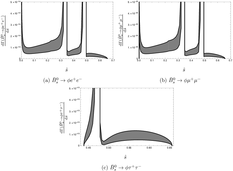
Considering the possible long-distance (LD) effects and to avoid the contributions of resonances, some cuts around the resonances of J/ψJ/\psi and ψ′\psi^{{}^{\prime}} are taken in the physical distribution of q2q^{2}. We use the same cuts as that used by LHCb Collaboration in Ref. 15AQ. There are three regions for B¯s0→ϕ​e+​e−\bar{B}_{s}^{0}\to\phi e^{+}e^{-} and B¯s0→ϕ​μ+​μ−\bar{B}_{s}^{0}\to\phi\mu^{+}\mu^{-} decays:

i:\displaystyle\mbox{i}: 0.1​GeV2≤q2≤8.0​GeV2;\displaystyle~0.1~{\rm GeV^{2}}\leq q^{2}\leq 8.0~{\rm GeV^{2}}~;
ii:\displaystyle\mbox{ii}: 11.0​GeV2≤q2≤12.5​GeV2;\displaystyle~11.0~{\rm GeV^{2}}\leq q^{2}\leq 12.5~{\rm GeV^{2}}~; (26)
iii:\displaystyle\mbox{iii}: 15.0​GeV2≤q2≤19.0​GeV2.\displaystyle~15.0~{\rm GeV^{2}}\leq q^{2}\leq 19.0~{\rm GeV^{2}}~.

and two regions for B¯s0→ϕ​τ+​τ−\bar{B}_{s}^{0}\to\phi\tau^{+}\tau^{-} decay:

i:\displaystyle\mbox{i}: 11.0​GeV2≤q2≤12.5​GeV2;\displaystyle~11.0~{\rm GeV^{2}}\leq q^{2}\leq 12.5~{\rm GeV^{2}}~;
ii:\displaystyle\mbox{ii}: 15.0​GeV2≤q2≤19.0​GeV2.\displaystyle~15.0~{\rm GeV^{2}}\leq q^{2}\leq 19.0~{\rm GeV^{2}}~. (27)
Refer to caption
Figure 4: The differential decay widths of B¯s0→ϕ​l+​l−\bar{B}_{s}^{0}\to\phi l^{+}l^{-} (l=e,μ,τl=e,\mu,\tau) on q2q^{2} with LD effects. The grey bands denote the relevant uncertainties.

The q2q^{2}-dependence of differential decay widths with long-distance (LD) effects are shown in Fig.4, where the grey bands denote the relevant uncertainties. Integrating the differential decay width in Eq. (25) with respect to q2q^{2} within the relevant region, we can obtain the value of integrated decay width Γ⁡(B¯s0→ϕ​l+​l−)\Gamma(\bar{B}^{0}_{s}\to\phi l^{+}l^{-}). According to the definition of decay branching ratio

Br​(B¯s0→ϕ​l+​l−)=Γ⁡(B¯s0→ϕ​l+​l−)Γtotal​(B¯s0),\displaystyle\mbox{Br}(\bar{B}^{0}_{s}\to\phi l^{+}l^{-})=\frac{\Gamma(\bar{B}^{0}_{s}\to\phi l^{+}l^{-})}{\Gamma_{{\rm total}}(\bar{B}^{0}_{s})}, (28)

and the total decay width of B¯s0\bar{B}_{s}^{0} meson: Γtotal​(B¯s0)=4.362×10⁻¹³​GeV\Gamma_{{\rm total}}(\bar{B}^{0}_{s})=4.362\times 10^{-13}\mbox{GeV} PDG2018, we can get the branching ratios of the three semileptonic decay channels of B¯s0→ϕ​l+​l−\bar{B}_{s}^{0}\to\phi l^{+}l^{-} (l=e,μ,τl=e,\mu,\tau),

Br​(B¯s0→ϕ​e+​e−)=(7.12±1.40)×10−7,\displaystyle\mbox{Br}(\bar{B}_{s}^{0}\to\phi e^{+}e^{-})=(7.12\pm 1.40)\times 10^{-7}, (29)
Br​(B¯s0→ϕ​μ+​μ−)=(7.06±1.59)×10−7,\displaystyle\mbox{Br}(\bar{B}_{s}^{0}\to\phi\mu^{+}\mu^{-})=(7.06\pm 1.59)\times 10^{-7}, (30)
Br​(B¯s0→ϕ​τ+​τ−)=(3.49±1.69)×10−8.\displaystyle\mbox{Br}(\bar{B}_{s}^{0}\to\phi\tau^{+}\tau^{-})=(3.49\pm 1.69)\times 10^{-8}. (31)

The experimental result of the total branching ratio of B¯s0→ϕ​μ+​μ−\bar{B}_{s}^{0}\to\phi\mu^{+}\mu^{-} is 15AQ

Br​(B¯s0→ϕ​μ+​μ−)=(7.97−0.43+0.45±0.22±0.23±0.60)×10−7.\mbox{Br}(\bar{B}_{s}^{0}\to\phi\mu^{+}\mu^{-})=(7.97^{+0.45}_{-0.43}\pm 0.22\pm 0.23\pm 0.60)\times 10^{-7}. (32)

We find agreement between our predictions and the experimental data within uncertainties.

Furthermore, in order to show the physical effects caused by the sign of the form factors, we change the sign of the form factors VV, A1A_{1}, T1T_{1} and T3T_{3} as that of Ref. R.K-SumR to calculate the branching ratio of B¯s0→ϕ​μ+​μ−\bar{B}_{s}^{0}\to\phi\mu^{+}\mu^{-} again, and obtain the central value of the branching ratio of as follows

Br​(B¯s0→ϕ​μ+​μ−)=6.14×10⁻⁶.\displaystyle\mbox{Br}(\bar{B}_{s}^{0}\to\phi\mu^{+}\mu^{-})=6.14\times 10^{-6}. (33)

From Eq. (33) we can find that the branching ratio of B¯s0→ϕ​μ+​μ−\bar{B}_{s}^{0}\to\phi\mu^{+}\mu^{-} calculated in this way is nearly an order of magnitude larger than the experimental data in Eq. (32). So the physical effect of the sign of the form factors are crucial.

VI Summary

We revisit the semi-leptonic decays of B¯s0→ϕ​l+​l−\bar{B}_{s}^{0}\to\phi l^{+}l^{-} (l=e,μ,τl=e,\mu,\tau) with QCD sum rule method. The B¯s0→ϕ\bar{B}_{s}^{0}\to\phi transition form factors VV, A0A_{0}, A1A_{1}, A2A_{2} PYQ and T1T_{1}, T2T_{2}, T3T_{3} are calculated, then they are used to obtain the branching ratios of B¯s0→ϕ​e+​e−\bar{B}_{s}^{0}\to\phi e^{+}e^{-}, B¯s0→ϕ​μ+​μ−\bar{B}_{s}^{0}\to\phi\mu^{+}\mu^{-} and B¯s0→ϕ​τ+​τ−\bar{B}_{s}^{0}\to\phi\tau^{+}\tau^{-} respectively. For the measured decay channel B¯s0→ϕ​μ+​μ−\bar{B}_{s}^{0}\to\phi\mu^{+}\mu^{-}, our theoretical result is Br​(B¯s0→ϕ​μ+​μ−)=(7.06±1.59)×10−7\mbox{Br}(\bar{B}_{s}^{0}\to\phi\mu^{+}\mu^{-})=(7.06\pm 1.59)\times 10^{-7}, which is well consistent with the latest experimental data Br​(B¯s0→ϕ​μ+​μ−)=(7.97−0.43+0.45±0.22±0.23±0.60)×10−7\mbox{Br}(\bar{B}_{s}^{0}\to\phi\mu^{+}\mu^{-})=(7.97^{+0.45}_{-0.43}\pm 0.22\pm 0.23\pm 0.60)\times 10^{-7} from LHCb Collaboration within uncertainties. For the unmeasured decay channels: B¯s0→ϕ​e+​e−\bar{B}_{s}^{0}\to\phi e^{+}e^{-} and B¯s0→ϕ​τ+​τ−\bar{B}_{s}^{0}\to\phi\tau^{+}\tau^{-}, we hope that our theoretical predictions are useful for experimental test in the future.

Acknowledgements.
This work is supported in part by the National Natural Science Foundation of China under Contracts No. 11875168 and No. 11375088. Appendix A The explicit form of the relevant Borel transformed Coefficients B^​κ0\hat{B}\kappa_{0}, 12​B^​(κ1−κ3)\frac{1}{2}\hat{B}(\kappa_{1}-\kappa_{3}) and B^​κ5\hat{B}\kappa_{5} in Eq. (III) are given in the following. 1) Results for Borel transformed κ0\kappa_{0}:
B^​κ0=B^​κ0pert+B^​κ0(3)+B^​κ0(4)+B^​κ0(5)+B^​κ0(6),\hat{B}\kappa_{0}=\hat{B}\kappa_{0}^{{\rm pert}}+\hat{B}\kappa_{0}^{(3)}+\hat{B}\kappa_{0}^{(4)}+\hat{B}\kappa_{0}^{(5)}+\hat{B}\kappa_{0}^{(6)}\;,

where

B^​κ0pert=∫s204​ms2ds2∫s10s1Lds13e−s1/M12−s2/M228​π2​λ3/2​M12​M22[−2λmbms+4s2mb2ms2−2s2mb4+s2(−λ−2ms4+q4−2q2s2+s12−2s1s2+s22)],\begin{array}[]{ll}\hat{B}\kappa_{0}^{{\rm pert}}~=&\int^{s_{2}^{0}}_{4m_{s}^{2}}{\rm d}s_{2}\int^{s_{1}^{0}}_{s_{1}^{L}}{\rm d}s_{1}\displaystyle\frac{3{\rm e}^{-s_{1}/M_{1}^{2}-s_{2}/M_{2}^{2}}}{8\pi^{2}\lambda^{3/2}M_{1}^{2}M_{2}^{2}}\left[-2\lambda m_{b}m_{s}+4s_{2}m_{b}^{2}m_{s}^{2}\right.\\ &\left.-2s_{2}m_{b}^{4}+s_{2}(-\lambda-2m_{s}^{4}+q^{4}-2q^{2}s_{2}+s_{1}^{2}-2s_{1}s_{2}+s_{2}^{2})\right],\end{array} (A​1)

with λ=(s1+s2−q2)2−4​s1​s2\lambda=(s_{1}+s_{2}-q^{2})^{2}-4s_{1}s_{2}.

B^​κ0(3)=e−mb2/M12−ms2/M226​M18​M28[M22mb3ms2(M12+M22)(3M12M22−ms2(M12+M22))+M12​M22​mb2​ms​(M22​ms2​(3​M12+3​M22+q2)−2​ms4​(M12+M22)−3​M12​M24)−M24​mb4​ms3​(M12+M22)+M12​mb​(M22​ms4​(M12+M22)​(4​M12+M22+q2)CLOSEOPEN−ms6​(M12+M22)2−3​M12​M24​ms2​(M12+M22+q2)+6​M14​M26)+M14​ms×(M24​ms2​(3​M12+2​q2)+M22​ms4​(3​M12+3​M22+q2)−ms6​(M12+M22)CLOSE+3M12M26)]×⟨s¯s⟩,\begin{array}[]{ll}\hat{B}\kappa_{0}^{(3)}~=&\displaystyle\frac{{\rm e}^{-m_{b}^{2}/M_{1}^{2}-m_{s}^{2}/M_{2}^{2}}}{6M_{1}^{8}M_{2}^{8}}[M_{2}^{2}m_{b}^{3}m_{s}^{2}(M_{1}^{2}+M_{2}^{2})(3M_{1}^{2}M_{2}^{2}-m_{s}^{2}(M_{1}^{2}+M_{2}^{2}))\\ &+M_{1}^{2}M_{2}^{2}m_{b}^{2}m_{s}(M_{2}^{2}m_{s}^{2}(3M_{1}^{2}+3M_{2}^{2}+q^{2})-2m_{s}^{4}(M_{1}^{2}+M_{2}^{2})-3M_{1}^{2}M_{2}^{4})\\ &-M_{2}^{4}m_{b}^{4}m_{s}^{3}(M_{1}^{2}+M_{2}^{2})+M_{1}^{2}m_{b}(M_{2}^{2}m_{s}^{4}(M_{1}^{2}+M_{2}^{2})(4M_{1}^{2}+M_{2}^{2}+q^{2})\\ &-m_{s}^{6}(M_{1}^{2}+M_{2}^{2})^{2}-3M_{1}^{2}M_{2}^{4}m_{s}^{2}(M_{1}^{2}+M_{2}^{2}+q^{2})+6M_{1}^{4}M_{2}^{6})+M_{1}^{4}m_{s}\\ &\times(M_{2}^{4}m_{s}^{2}(3M_{1}^{2}+2q^{2})+M_{2}^{2}m_{s}^{4}(3M_{1}^{2}+3M_{2}^{2}+q^{2})-m_{s}^{6}(M_{1}^{2}+M_{2}^{2})\\ &+3M_{1}^{2}M_{2}^{6})]\times\langle\bar{s}s\rangle\;,\end{array} (A​2)
B^​κ0(4)=−∫s204​ms2ds2∫s10s1Lds1e−s1/M12−s2/M2296​π2​λ3/2​M12​M22(−4q2+5s1+4s2)×4παs⟨GG⟩,\begin{array}[]{ll}\hat{B}\kappa_{0}^{(4)}~=&-\int^{s_{2}^{0}}_{4m_{s}^{2}}{\rm d}s_{2}\int^{s_{1}^{0}}_{s_{1}^{L}}{\rm d}s_{1}\displaystyle\frac{{\rm e}^{-s_{1}/M_{1}^{2}-s_{2}/M_{2}^{2}}}{96\pi^{2}\lambda^{3/2}M_{1}^{2}M_{2}^{2}}(-4q^{2}+5s_{1}+4s_{2})\times 4\pi\alpha_{s}\langle GG\rangle\;,\end{array} (A​3)
B^​κ0(5)=−e−mb2/M12−ms2/M2212​M18​M28[M12M22mb2ms(M22(3M12+q2)−2ms2(M12+M22))+M22​mb3​(M12+M22)​(3​M12​M22−ms2​(M12+M22))+M12​mb​(M22​ms2​(M12CLOSECLOSEOPENOPEN+M22)​(5​M12−2​M22+q2)−ms4​(M12+M22)2+M12​M24​(M12−6​M22−3​q2))−M24​mb4​ms​(M12+M22)+M14​ms​(M22​ms2​(4​M12+M22+q2)−ms4​(M12+M22)CLOSE−M24(−2M12+3M22+q2))]×g⟨s¯σTGs⟩,\begin{array}[]{ll}\hat{B}\kappa_{0}^{(5)}~=&-\displaystyle\frac{{\rm e}^{-m_{b}^{2}/M_{1}^{2}-m_{s}^{2}/M_{2}^{2}}}{12M_{1}^{8}M_{2}^{8}}[M_{1}^{2}M_{2}^{2}m_{b}^{2}m_{s}(M_{2}^{2}(3M_{1}^{2}+q^{2})-2m_{s}^{2}(M_{1}^{2}+M_{2}^{2}))\\ &+M_{2}^{2}m_{b}^{3}(M_{1}^{2}+M_{2}^{2})(3M_{1}^{2}M_{2}^{2}-m_{s}^{2}(M_{1}^{2}+M_{2}^{2}))+M_{1}^{2}m_{b}(M_{2}^{2}m_{s}^{2}(M_{1}^{2}\\ &+M_{2}^{2})(5M_{1}^{2}-2M_{2}^{2}+q^{2})-m_{s}^{4}(M_{1}^{2}+M_{2}^{2})^{2}+M_{1}^{2}M_{2}^{4}(M_{1}^{2}-6M_{2}^{2}-3q^{2}))\\ &-M_{2}^{4}m_{b}^{4}m_{s}(M_{1}^{2}+M_{2}^{2})+M_{1}^{4}m_{s}(M_{2}^{2}m_{s}^{2}(4M_{1}^{2}+M_{2}^{2}+q^{2})-m_{s}^{4}(M_{1}^{2}+M_{2}^{2})\\ &-M_{2}^{4}(-2M_{1}^{2}+3M_{2}^{2}+q^{2}))]\times g\langle\bar{s}\sigma TGs\rangle\;,\end{array} (A​4)
B^​κ0(6)=−e−mb2/M12−ms2/M2281​M18​M28​ms3​(mb2−q2)[M22mb5ms4(M12+M22)2+M24mb6ms3(M12+M22)+M22​mb4​ms3​(2​M12​ms2​(M12+M22)−M22​(−3​M14+M12​(15​M22+2​q2)+M22​q2))+M12​mb2​ms​(18​M14​M26​(ems2M22−1)+M12​ms6​(M12+M22)−M22​ms4​(M14+3​M12CLOSECLOSE×(3M22+q2)+2M22q2)+M24ms2(50M14−4M12(6M22+q2)+q2(15M22+q2)))+M12​mb​(54​M14​M26​q2​(ems2M22−1)−18​M14​M24​ms2​(M22​(ems2M22−1)+3​q2)−q2​ms6CLOSE×(M12+M22)2+M22q2ms4(M14+M12(20M22+q2)+M22(13M22+q2)))−mb3×(−54​M16​M24​ms2+54​M16​M26​(ems2M22−1)−M12​ms6​(M12+M22)2+M22​ms4​(M16CLOSECLOSEOPENOPEN+2​M14​(10​M22+q2)+M12​(13​M24+3​M22​q2)+M24​q2))+M14​q2​ms​(M22​ms4​(M12CLOSECLOSEOPEN+9​M22+q2)−ms6​(M12+M22)+18​M12​M26​(ems2M22−1)+M24​ms2​(−50​M12+24​M22CLOSE+q2))]×g2⟨s¯s⟩2.\begin{array}[]{ll}\hat{B}\kappa_{0}^{(6)}~=&\displaystyle-\frac{{\rm e}^{-m_{b}^{2}/M_{1}^{2}-m_{s}^{2}/M_{2}^{2}}}{81M_{1}^{8}M_{2}^{8}m_{s}^{3}(m_{b}^{2}-q^{2})}[M_{2}^{2}m_{b}^{5}m_{s}^{4}(M_{1}^{2}+M_{2}^{2})^{2}+M_{2}^{4}m_{b}^{6}m_{s}^{3}(M_{1}^{2}+M_{2}^{2})\\ &+M_{2}^{2}m_{b}^{4}m_{s}^{3}(2M_{1}^{2}m_{s}^{2}(M_{1}^{2}+M_{2}^{2})-M_{2}^{2}(-3M_{1}^{4}+M_{1}^{2}(15M_{2}^{2}+2q^{2})+M_{2}^{2}q^{2}))\\ &+M_{1}^{2}m_{b}^{2}m_{s}(18M_{1}^{4}M_{2}^{6}({\rm e}^{\frac{m_{s}^{2}}{M_{2}^{2}}}-1)+M_{1}^{2}m_{s}^{6}(M_{1}^{2}+M_{2}^{2})-M_{2}^{2}m_{s}^{4}(M_{1}^{4}+3M_{1}^{2}\\ &\times(3M_{2}^{2}+q^{2})+2M_{2}^{2}q^{2})+M_{2}^{4}m_{s}^{2}(50M_{1}^{4}-4M_{1}^{2}(6M_{2}^{2}+q^{2})+q^{2}(15M_{2}^{2}+q^{2})))\\ &+M_{1}^{2}m_{b}(54M_{1}^{4}M_{2}^{6}q^{2}(e^{\frac{m_{s}^{2}}{M_{2}^{2}}}-1)-18M_{1}^{4}M_{2}^{4}m_{s}^{2}(M_{2}^{2}({\rm e}^{\frac{m_{s}^{2}}{M_{2}^{2}}}-1)+3q^{2})-q^{2}m_{s}^{6}\\ &\times(M_{1}^{2}+M_{2}^{2})^{2}+M_{2}^{2}q^{2}m_{s}^{4}(M_{1}^{4}+M_{1}^{2}(20M_{2}^{2}+q^{2})+M_{2}^{2}(13M_{2}^{2}+q^{2})))-m_{b}^{3}\\ &\times(-54M_{1}^{6}M_{2}^{4}m_{s}^{2}+54M_{1}^{6}M_{2}^{6}({\rm e}^{\frac{m_{s}^{2}}{M_{2}^{2}}}-1)-M_{1}^{2}m_{s}^{6}(M_{1}^{2}+M_{2}^{2})^{2}+M_{2}^{2}m_{s}^{4}(M_{1}^{6}\\ &+2M_{1}^{4}(10M_{2}^{2}+q^{2})+M_{1}^{2}(13M_{2}^{4}+3M_{2}^{2}q^{2})+M_{2}^{4}q^{2}))+M_{1}^{4}q^{2}m_{s}(M_{2}^{2}m_{s}^{4}(M_{1}^{2}\\ &+9M_{2}^{2}+q^{2})-m_{s}^{6}(M_{1}^{2}+M_{2}^{2})+18M_{1}^{2}M_{2}^{6}({\rm e}^{\frac{m_{s}^{2}}{M_{2}^{2}}}-1)+M_{2}^{4}m_{s}^{2}(-50M_{1}^{2}+24M_{2}^{2}\\ &+q^{2}))]\times g^{2}\langle\bar{s}s\rangle^{2}\;.\end{array} (A​5)

In the perturbative diagram, we consider the condition that all internal quarks are on their mass shell R1, which gives the lower limit of the integration s1Ls_{1}^{L} as

s1L=mb2mb2−q2​s2+mb2,s_{1}^{L}=\frac{m_{b}^{2}}{m_{b}^{2}-q^{2}}s_{2}+m_{b}^{2},

2) Results for Borel transformed (κ1−κ3)(\kappa_{1}-\kappa_{3}) :

12​B^​(κ1−κ3)=12​B^​κ−pert+12​B^​κ−(3)+12​B^​κ−(4)+12​B^​κ−(5)+12​B^​κ−(6),\frac{1}{2}\hat{B}(\kappa_{1}-\kappa_{3})=\frac{1}{2}\hat{B}\kappa_{-}^{{\rm pert}}+\frac{1}{2}\hat{B}\kappa_{-}^{(3)}+\frac{1}{2}\hat{B}\kappa_{-}^{(4)}+\frac{1}{2}\hat{B}\kappa_{-}^{(5)}+\frac{1}{2}\hat{B}\kappa_{-}^{(6)}\;,
12​B^​κ−pert=−∫s204​ms2ds2∫s10s1Lds13e−s1/M12−s2/M228​π2​λ5/2​M12​M22[s2mb4(2λ−3q4+12q2s2+3s12+6s1s2OPEN−9​s22)−2​s2​mb2​(ms2​(2​λ−3​q4+12​q2​s2+3​s12+6​s1​s2−9​s22)−q6CLOSE−2​q4​(s1−3​s2)+q2​(λ+s12+8​s1​s2−9​s22)+2​(s13−3​s1​s22+2​s23CLOSEOPENOPEN−λ​s2))+λ2​mb​ms+s2​ms4​(2​λ−3​q4+12​q2​s2+3​s12+6​s1​s2−9​s22)+ms2​(−λ2−2​q6​s2−q4​(λ+4​s1​s2−12​s22)+2​q2​s2​(3​λ+s12+8​s1​s2CLOSECLOSEOPENOPEN−9​s22)+4​s13​s2+λ​s12+2​s1​s2​(λ−6​s22)+8​s24−7​λ​s22)+s2​(Q3​(s2CLOSECLOSEOPEN−2​s1)−q4​(s12−8​s1​s2+3​s22)+q2​(s1−s2)​(λ+2​s12+5​s1​s2−3​s22)+(s12−s22)(−λ+s12−2s1s2+s22))],\begin{array}[]{ll}\frac{1}{2}\hat{B}\kappa_{-}^{{\rm pert}}~=&-\int^{s_{2}^{0}}_{4m_{s}^{2}}{\rm d}s_{2}\int^{s_{1}^{0}}_{s_{1}^{L}}{\rm d}s_{1}\displaystyle\frac{3{\rm e}^{-s_{1}/M_{1}^{2}-s_{2}/M_{2}^{2}}}{8\pi^{2}\lambda^{5/2}M_{1}^{2}M_{2}^{2}}[s_{2}m_{b}^{4}(2\lambda-3q^{4}+12q^{2}s_{2}+3s_{1}^{2}+6s_{1}s_{2}\\ &-9s_{2}^{2})-2s_{2}m_{b}^{2}(m_{s}^{2}(2\lambda-3q^{4}+12q^{2}s_{2}+3s_{1}^{2}+6s_{1}s_{2}-9s_{2}^{2})-q^{6}\\ &-2q^{4}(s_{1}-3s_{2})+q^{2}(\lambda+s_{1}^{2}+8s_{1}s_{2}-9s_{2}^{2})+2(s_{1}^{3}-3s_{1}s_{2}^{2}+2s_{2}^{3}\\ &-\lambda s_{2}))+\lambda^{2}m_{b}m_{s}+s_{2}m_{s}^{4}(2\lambda-3q^{4}+12q^{2}s_{2}+3s_{1}^{2}+6s_{1}s_{2}-9s_{2}^{2})\\ &+m_{s}^{2}(-\lambda^{2}-2q^{6}s_{2}-q^{4}(\lambda+4s_{1}s_{2}-12s_{2}^{2})+2q^{2}s_{2}(3\lambda+s_{1}^{2}+8s_{1}s_{2}\\ &-9s_{2}^{2})+4s_{1}^{3}s_{2}+\lambda s_{1}^{2}+2s_{1}s_{2}(\lambda-6s_{2}^{2})+8s_{2}^{4}-7\lambda s_{2}^{2})+s_{2}(Q^{3}(s_{2}\\ &-2s_{1})-q^{4}(s_{1}^{2}-8s_{1}s_{2}+3s_{2}^{2})+q^{2}(s_{1}-s_{2})(\lambda+2s_{1}^{2}+5s_{1}s_{2}-3s_{2}^{2})\\ &+(s_{1}^{2}-s_{2}^{2})(-\lambda+s_{1}^{2}-2s_{1}s_{2}+s_{2}^{2}))],\end{array} (A​6)
12​B^​κ−(3)=−e−mb2/M12−ms2/M2212​M18​M28[−M22mb3ms2(M12+M22)(ms2(M22−M12)+3M12×M22)+M12M24mb2ms(ms2(5M12+M22−q2)+3M12M22)+M24×mb4​ms3​(M12+M22)+M12​mb​(ms6​(M14−M24)+3​M12​M24​ms2​(M12CLOSECLOSEOPEN+M22+q2)+M22​ms4​(−4​M14−M12​(3​M22+q2)+M22​(M22+q2))OPEN−6​M14​M26)+M14​ms​(−M24​ms2​(9​M12+4​q2)+M22​ms4​(7​M12+3​M22CLOSECLOSE+q2)−ms6(M12+M22)+9M12M26)]×⟨s¯s⟩,\begin{array}[]{ll}\frac{1}{2}\hat{B}\kappa_{-}^{(3)}~=&-\displaystyle\frac{{\rm e}^{-m_{b}^{2}/M_{1}^{2}-m_{s}^{2}/M_{2}^{2}}}{12M_{1}^{8}M_{2}^{8}}[-M_{2}^{2}m_{b}^{3}m_{s}^{2}(M_{1}^{2}+M_{2}^{2})(m_{s}^{2}(M_{2}^{2}-M_{1}^{2})+3M_{1}^{2}\\ &\times M_{2}^{2})+M_{1}^{2}M_{2}^{4}m_{b}^{2}m_{s}(m_{s}^{2}(5M_{1}^{2}+M_{2}^{2}-q^{2})+3M_{1}^{2}M_{2}^{2})+M_{2}^{4}\\ &\times m_{b}^{4}m_{s}^{3}(M_{1}^{2}+M_{2}^{2})+M_{1}^{2}m_{b}(m_{s}^{6}(M_{1}^{4}-M_{2}^{4})+3M_{1}^{2}M_{2}^{4}m_{s}^{2}(M_{1}^{2}\\ &+M_{2}^{2}+q^{2})+M_{2}^{2}m_{s}^{4}(-4M_{1}^{4}-M_{1}^{2}(3M_{2}^{2}+q^{2})+M_{2}^{2}(M_{2}^{2}+q^{2}))\\ &-6M_{1}^{4}M_{2}^{6})+M_{1}^{4}m_{s}(-M_{2}^{4}m_{s}^{2}(9M_{1}^{2}+4q^{2})+M_{2}^{2}m_{s}^{4}(7M_{1}^{2}+3M_{2}^{2}\\ &+q^{2})-m_{s}^{6}(M_{1}^{2}+M_{2}^{2})+9M_{1}^{2}M_{2}^{6})]\times\langle\bar{s}s\rangle\;,\end{array} (A​7)
12​B^​κ−(4)=∫s204​ms2ds2∫s10s1Lds1e−s1/M12−s2/M2296​π2​λ5/2​M​12​M​22[3q6−3q4(5s1+3s2)+q2(−5λOPEN+21​s12+22​s1​s2+9​s22)−9​s13−13​s12​s2+4​λ​s1+25​s1​s22−3​s23+9λs2]×4παs⟨GG⟩,\begin{array}[]{ll}\frac{1}{2}\hat{B}\kappa_{-}^{(4)}~=&\int^{s_{2}^{0}}_{4m_{s}^{2}}{\rm d}s_{2}\int^{s_{1}^{0}}_{s_{1}^{L}}{\rm d}s_{1}\displaystyle\frac{{\rm e}^{-s_{1}/M_{1}^{2}-s_{2}/M_{2}^{2}}}{96\pi^{2}\lambda^{5/2}M1^{2}M2^{2}}[3q^{6}-3q^{4}(5s_{1}+3s_{2})+q^{2}(-5\lambda\\ &+21s_{1}^{2}+22s_{1}s_{2}+9s_{2}^{2})-9s_{1}^{3}-13s_{1}^{2}s_{2}+4\lambda s_{1}+25s_{1}s_{2}^{2}-3s_{2}^{3}\\ &+9\lambda s_{2}]\times 4\pi\alpha_{s}\langle GG\rangle\;,\end{array} (A​8)
12​B^​κ+(5)=−e−mb2/M12−ms2/M2224​M18​M28[M22mb3(M12+M22)(ms2(M22−M12)+3M12M22)+M12​M24​mb2​ms​(−7​M12−4​M22+q2)−M24​mb4​ms​(M12+M22)+M12×mb​(ms4​(M24−M14)+M22​ms2​(5​M14+M12​(q2−M22)+2​M24−M22CLOSECLOSE×q2)+M12M24(M12−3(4M22+q2)))+M14ms(−M22ms2(8M12+M22+q2)+ms4(M12+M22)+M24(8M12+3M22+5q2))]×g⟨s¯σTGs⟩,\begin{array}[]{ll}\frac{1}{2}\hat{B}\kappa_{+}^{(5)}~=&-\displaystyle\frac{{\rm e}^{-m_{b}^{2}/M_{1}^{2}-m_{s}^{2}/M_{2}^{2}}}{24M_{1}^{8}M_{2}^{8}}[M_{2}^{2}m_{b}^{3}(M_{1}^{2}+M_{2}^{2})(m_{s}^{2}(M_{2}^{2}-M_{1}^{2})+3M_{1}^{2}M_{2}^{2})\\ &+M_{1}^{2}M_{2}^{4}m_{b}^{2}m_{s}(-7M_{1}^{2}-4M_{2}^{2}+q^{2})-M_{2}^{4}m_{b}^{4}m_{s}(M_{1}^{2}+M_{2}^{2})+M_{1}^{2}\\ &\times m_{b}(m_{s}^{4}(M_{2}^{4}-M_{1}^{4})+M_{2}^{2}m_{s}^{2}(5M_{1}^{4}+M_{1}^{2}(q^{2}-M_{2}^{2})+2M_{2}^{4}-M_{2}^{2}\\ &\times q^{2})+M_{1}^{2}M_{2}^{4}(M_{1}^{2}-3(4M_{2}^{2}+q^{2})))+M_{1}^{4}m_{s}(-M_{2}^{2}m_{s}^{2}(8M_{1}^{2}+M_{2}^{2}\\ &+q^{2})+m_{s}^{4}(M_{1}^{2}+M_{2}^{2})+M_{2}^{4}(8M_{1}^{2}+3M_{2}^{2}+5q^{2}))]\times g\langle\bar{s}\sigma TGs\rangle\;,\end{array} (A​9)
12​B^​κ+(6)=−e−mb2/M12−ms2/M22162​M18​M28​ms3​(mb2−q2)[M22mb5ms4(M14−M24)+M24mb6ms3(M12OPEN+M22)−M24​mb4​ms3​(−5​M14+M12​(17​M22+2​q2)+M22​q2)+M12×mb2​ms​(54​M14​M26​(ems2M22−1)+M12​M22​ms4​(5​M12+9​M22+q2)CLOSE−M12​ms6​(M12+M22)+M24​ms2​(−44​M14−6​M12​(4​M22+q2)+q2CLOSE×(17M22+q2)))+M12mb(q2ms6(M24−M14)+54M14M26q2(ems2M22−1)−18​M14​M24​ms2​(M22​(ems2M22−1)+3​q2)+M22​q2​ms4​(M14+M12​(18​M22CLOSECLOSE+q2)−M22(13M22+q2)))+mb3(54M16M24ms2−54M16M26(ems2M22−1)+ms6​(M16−M12​M24)+M22​ms4​(−M16−2​M14​(9​M22+q2)+M12​M22CLOSE×(13M22+q2)+M24q2))+M14ms(−M22q2ms4(5M12+9M22+q2)+q2​ms6​(M12+M22)−54​M12​M26​q2​(ems2M22−1)+M24​ms2​(M12​(44​q2−72CLOSECLOSE×M22)+q2(24M22+q2)))]×g2⟨s¯s⟩2.\begin{array}[]{ll}\frac{1}{2}\hat{B}\kappa_{+}^{(6)}~=&-\displaystyle\frac{{\rm e}^{-m_{b}^{2}/M_{1}^{2}-m_{s}^{2}/M_{2}^{2}}}{162M_{1}^{8}M_{2}^{8}m_{s}^{3}(m_{b}^{2}-q^{2})}[M_{2}^{2}m_{b}^{5}m_{s}^{4}(M_{1}^{4}-M_{2}^{4})+M_{2}^{4}m_{b}^{6}m_{s}^{3}(M_{1}^{2}\\ &+M_{2}^{2})-M_{2}^{4}m_{b}^{4}m_{s}^{3}(-5M_{1}^{4}+M_{1}^{2}(17M_{2}^{2}+2q^{2})+M_{2}^{2}q^{2})+M_{1}^{2}\\ &\times m_{b}^{2}m_{s}(54M_{1}^{4}M_{2}^{6}({\rm e}^{\frac{m_{s}^{2}}{M_{2}^{2}}}-1)+M_{1}^{2}M_{2}^{2}m_{s}^{4}(5M_{1}^{2}+9M_{2}^{2}+q^{2})\\ &-M_{1}^{2}m_{s}^{6}(M_{1}^{2}+M_{2}^{2})+M_{2}^{4}m_{s}^{2}(-44M_{1}^{4}-6M_{1}^{2}(4M_{2}^{2}+q^{2})+q^{2}\\ &\times(17M_{2}^{2}+q^{2})))+M_{1}^{2}m_{b}(q^{2}m_{s}^{6}(M_{2}^{4}-M_{1}^{4})+54M_{1}^{4}M_{2}^{6}q^{2}({\rm e}^{\frac{m_{s}^{2}}{M_{2}^{2}}}-1)\\ &-18M_{1}^{4}M_{2}^{4}m_{s}^{2}(M_{2}^{2}({\rm e}^{\frac{m_{s}^{2}}{M_{2}^{2}}}-1)+3q^{2})+M_{2}^{2}q^{2}m_{s}^{4}(M_{1}^{4}+M_{1}^{2}(18M_{2}^{2}\\ &+q^{2})-M_{2}^{2}(13M_{2}^{2}+q^{2})))+m_{b}^{3}(54M_{1}^{6}M_{2}^{4}m_{s}^{2}-54M_{1}^{6}M_{2}^{6}({\rm e}^{\frac{m_{s}^{2}}{M_{2}^{2}}}-1)\\ &+m_{s}^{6}(M_{1}^{6}-M_{1}^{2}M_{2}^{4})+M_{2}^{2}m_{s}^{4}(-M_{1}^{6}-2M_{1}^{4}(9M_{2}^{2}+q^{2})+M_{1}^{2}M_{2}^{2}\\ &\times(13M_{2}^{2}+q^{2})+M_{2}^{4}q^{2}))+M_{1}^{4}m_{s}(-M_{2}^{2}q^{2}m_{s}^{4}(5M_{1}^{2}+9M_{2}^{2}+q^{2})\\ &+q^{2}m_{s}^{6}(M_{1}^{2}+M_{2}^{2})-54M_{1}^{2}M_{2}^{6}q^{2}({\rm e}^{\frac{m_{s}^{2}}{M_{2}^{2}}}-1)+M_{2}^{4}m_{s}^{2}(M_{1}^{2}(44q^{2}-72\\ &\times M_{2}^{2})+q^{2}(24M_{2}^{2}+q^{2})))]\times g^{2}\langle\bar{s}s\rangle^{2}\;.\end{array} (A​10)

3) Results for Borel transformed κ5\kappa_{5} :

B^​κ5pert=−∫s204​ms2ds2∫s10s1Lds13e−s1/M12−s2/M228​π2​λ3/2​M12​M22[−s2mb2(−λ+2ms2(q2+s1−s2)OPEN+q4+2​q2​(s1−s2)+s12−2​s1​s2+s22)−λ​mb​ms​(q2−s1+s2)+s2​mb4​(q2+s1−s2)+ms2​(q4​s2+2​q2​(λ+s1​s2−s22)+s2​(−λ+s12CLOSECLOSE−2s1s2+s22))+s2ms4(q2+s1−s2)+q2s1s2(q2+s1−s2)],\begin{array}[]{ll}\hat{B}\kappa_{5}^{{\rm pert}}~=&-\int^{s_{2}^{0}}_{4m_{s}^{2}}{\rm d}s_{2}\int^{s_{1}^{0}}_{s_{1}^{L}}{\rm d}s_{1}\displaystyle\frac{3{\rm e}^{-s_{1}/M_{1}^{2}-s_{2}/M_{2}^{2}}}{8\pi^{2}\lambda^{3/2}M_{1}^{2}M_{2}^{2}}[-s_{2}m_{b}^{2}(-\lambda+2m_{s}^{2}(q^{2}+s_{1}-s_{2})\\ &+q^{4}+2q^{2}(s_{1}-s_{2})+s_{1}^{2}-2s_{1}s_{2}+s_{2}^{2})-\lambda m_{b}m_{s}(q^{2}-s_{1}+s_{2})\\ &+s_{2}m_{b}^{4}(q^{2}+s_{1}-s_{2})+m_{s}^{2}(q^{4}s_{2}+2q^{2}(\lambda+s_{1}s_{2}-s_{2}^{2})+s_{2}(-\lambda+s_{1}^{2}\\ &-2s_{1}s_{2}+s_{2}^{2}))+s_{2}m_{s}^{4}(q^{2}+s_{1}-s_{2})+q^{2}s_{1}s_{2}(q^{2}+s_{1}-s_{2})]\;,\end{array} (A​11)
B^​κ5(3)=e−mb2/M12−ms2/M2212​M18​M28[M22mb5ms2(M12+M22)(3M12M22−ms2(M12OPENOPEN+M22))−M24​mb6​ms3​(M12+M22)+M12​mb2​ms​(M22​ms4​(M12−M22)CLOSE×(5​M12+5​M22+q2)−M24​ms2​(6​M14+M12​q2−2​M22​q2+q4)+ms6×(−M14+M12M22+2M24)+3M12M26(2M12+q2))+M12mb(−ms6×(M12+M22)​(M12​(5​M22−q2)+2​M22​(M22+q2))+ms8​(M12+M22)2+3​M12​M24​ms2​(q4−2​M12​(M22−q2))+M22​ms4​(M14​(6​M22−5​q2)CLOSEOPENOPEN+M12​(6​M24−q4)+M22​q2​(2​M22+q2))−6​M14​M26​q2)+mb4​(−3​M14CLOSE×M26​ms+M24​ms3​(5​M14+M12​(5​M22+2​q2)+M22​q2)+ms5​(−2​M14​M22CLOSEOPENOPEN−M12​M24+M26))+mb3​(−ms6​(M12−M22)​(M12+M22)2−M22​ms4​(M12CLOSECLOSEOPEN+M22)​(−5​M14+M12​(M22−2​q2)+M22​q2)−3​M12​M24​ms2​(2​M14+2​M12CLOSE×(M22+q2)+M22q2)+6M16M26)+M14ms(ms8(M12+M22)+M22ms4×(6​M12​(M22+q2)+3​M24+9​M22​q2+q4)−ms6​(M12​(5​M22+q2)+5​M24CLOSE+2M22q2)−M24ms2(M12(6M22+5q2)+4q2(M22+q2))+9M12M26q2)]×⟨s¯​s⟩,\begin{array}[]{ll}\hat{B}\kappa_{5}^{(3)}~=&\displaystyle\frac{{\rm e}^{-m_{b}^{2}/M_{1}^{2}-m_{s}^{2}/M_{2}^{2}}}{12M_{1}^{8}M_{2}^{8}}[M_{2}^{2}m_{b}^{5}m_{s}^{2}(M_{1}^{2}+M_{2}^{2})(3M_{1}^{2}M_{2}^{2}-m_{s}^{2}(M_{1}^{2}\\ &+M_{2}^{2}))-M_{2}^{4}m_{b}^{6}m_{s}^{3}(M_{1}^{2}+M_{2}^{2})+M_{1}^{2}m_{b}^{2}m_{s}(M_{2}^{2}m_{s}^{4}(M_{1}^{2}-M_{2}^{2})\\ &\times(5M_{1}^{2}+5M_{2}^{2}+q^{2})-M_{2}^{4}m_{s}^{2}(6M_{1}^{4}+M_{1}^{2}q^{2}-2M_{2}^{2}q^{2}+q^{4})+m_{s}^{6}\\ &\times(-M_{1}^{4}+M_{1}^{2}M_{2}^{2}+2M_{2}^{4})+3M_{1}^{2}M_{2}^{6}(2M_{1}^{2}+q^{2}))+M_{1}^{2}m_{b}(-m_{s}^{6}\\ &\times(M_{1}^{2}+M_{2}^{2})(M_{1}^{2}(5M_{2}^{2}-q^{2})+2M_{2}^{2}(M_{2}^{2}+q^{2}))+m_{s}^{8}(M_{1}^{2}+M_{2}^{2})^{2}\\ &+3M_{1}^{2}M_{2}^{4}m_{s}^{2}(q^{4}-2M_{1}^{2}(M_{2}^{2}-q^{2}))+M_{2}^{2}m_{s}^{4}(M_{1}^{4}(6M_{2}^{2}-5q^{2})\\ &+M_{1}^{2}(6M_{2}^{4}-q^{4})+M_{2}^{2}q^{2}(2M_{2}^{2}+q^{2}))-6M_{1}^{4}M_{2}^{6}q^{2})+m_{b}^{4}(-3M_{1}^{4}\\ &\times M_{2}^{6}m_{s}+M_{2}^{4}m_{s}^{3}(5M_{1}^{4}+M_{1}^{2}(5M_{2}^{2}+2q^{2})+M_{2}^{2}q^{2})+m_{s}^{5}(-2M_{1}^{4}M_{2}^{2}\\ &-M_{1}^{2}M_{2}^{4}+M_{2}^{6}))+m_{b}^{3}(-m_{s}^{6}(M_{1}^{2}-M_{2}^{2})(M_{1}^{2}+M_{2}^{2})^{2}-M_{2}^{2}m_{s}^{4}(M_{1}^{2}\\ &+M_{2}^{2})(-5M_{1}^{4}+M_{1}^{2}(M_{2}^{2}-2q^{2})+M_{2}^{2}q^{2})-3M_{1}^{2}M_{2}^{4}m_{s}^{2}(2M_{1}^{4}+2M_{1}^{2}\\ &\times(M2^{2}+q^{2})+M_{2}^{2}q^{2})+6M_{1}^{6}M_{2}^{6})+M_{1}^{4}m_{s}(m_{s}^{8}(M_{1}^{2}+M_{2}^{2})+M_{2}^{2}m_{s}^{4}\\ &\times(6M_{1}^{2}(M_{2}^{2}+q^{2})+3M_{2}^{4}+9M_{2}^{2}q^{2}+q^{4})-m_{s}^{6}(M_{1}^{2}(5M_{2}^{2}+q^{2})+5M_{2}^{4}\\ &+2M2^{2}q^{2})-M_{2}^{4}m_{s}^{2}(M_{1}^{2}(6M_{2}^{2}+5q^{2})+4q^{2}(M_{2}^{2}+q^{2}))+9M_{1}^{2}M_{2}^{6}q^{2})]\\ &\times\langle\bar{s}s\rangle\;,\end{array} (A​12)
B^​κ5(4)=−∫s204​ms2ds2∫s10s1Lds1e−s1/M12−s2/M22192​π2​λ3/2​M12​M22[−5λ+q4−2q2(3s1+s2)+5s12−6s1s2+s22]×4παs⟨GG⟩,\begin{array}[]{ll}\hat{B}\kappa_{5}^{(4)}~=&-\int^{s_{2}^{0}}_{4m_{s}^{2}}{\rm d}s_{2}\int^{s_{1}^{0}}_{s_{1}^{L}}{\rm d}s_{1}\displaystyle\frac{{\rm e}^{-s_{1}/M_{1}^{2}-s_{2}/M_{2}^{2}}}{192\pi^{2}\lambda^{3/2}M_{1}^{2}M_{2}^{2}}[-5\lambda+q^{4}-2q^{2}(3s_{1}+s_{2})+5s_{1}^{2}\\ &-6s_{1}s_{2}+s_{2}^{2}]\times 4\pi\alpha_{s}\langle GG\rangle\;,\end{array} (A​13)
B^​κ5(6)=e−mb2/M12−ms2/M22162​M18​M28​(mb2−q2)​ms3[−M24(M12+M22)ms3mb8−M22(M12+M22)2×ms4​mb7+M22​ms3​((−M14+(17​M22+3​q2)​M12+2​M22​q2)​M22+(−2​M14CLOSECLOSEOPENOPEN−M22​M12+M24)​ms2)​mb6+(54​(−1+ems2M22)​M26​M16−54​M24​ms2​M16+M22CLOSE×(2​M14+(22​M22+3​q2)​M12+14​M24+3​M22​q2)​ms4​M12−(M12−M22)×(M12+M22)2ms6)mb5−ms(18(−1+ems2M22)M16M26+(53M16+(9M22OPENOPEN−3​q2)​M14+3​q2​(11​M22+q2)​M12+M22​q4)​ms2​M24+(−3​M16−3​(4​M22CLOSECLOSE+q2)M14+17M24M12+M24q2)ms4M22+(M16−M22M14−2M24M12)ms6)×mb4+(M12(M12+M22)2ms8−(2(M22−q2)M16+22M24M14+(14M26OPENOPEN+3​q2​M24)​M12+M26​q2)​ms6+M22​((54​M22−4​q2)​M16−(60​M24+40​q2​M22CLOSECLOSEOPENOPEN+3​q4)​M14+M24​q4)​ms4+18​M16​M​24​((−1+ems2M22)​M22+6​q2)​ms2−108×(−1+ems2M22)M16M26q2)mb3+M12ms(M12(M12+M22)ms8−M22(3M14+OPEN(11​M22+3​q2)​M12+2​M22​q2)​ms6+(9​M12​M26+q2​(17​M22+q2)​M24+M14CLOSE×(49M22+q2)M22)ms4+M24((4q2−98M22)M14−q2(16M22+3q2)M12OPENOPEN+q4​(16​M22+q2))​ms2+72​(−1+ems2M22)​M14​M26​q2)​mb2+M12​(−(M12+M22)2CLOSEq2​ms8+q2​((2​M22−q2)​M14+M22​(22​M22+q2)​M12+2​M24​(7​M22+q2))​ms6+M22​(2​(9​M24−27​q2​M22+q4)​M14+q2​(60​M24+18​q2​M22+q4)​M12−M22​q4CLOSE×(14M22+q2))ms4−18M14M24q2((−1+ems2M22)M22+3q2)ms2+54(−1+ems2M22)×M14M26q4)mb+M14q2ms(−(M12+M22)ms8+(11M24+2q2M22+M12×(3M22+q2))ms6−M22(9M24+12q2M22+q4+M12(49M22+4q2))ms4+M24((26M22+49q2)M12+q2(25M22+q2))ms2−54(−1+ems2M22)M12M26q2)]×g2​⟨s¯​s⟩2.\begin{array}[]{ll}\hat{B}\kappa_{5}^{(6)}~=&\displaystyle\frac{{\rm e}^{-m_{b}^{2}/M_{1}^{2}-m_{s}^{2}/M_{2}^{2}}}{162M_{1}^{8}M_{2}^{8}(m_{b}^{2}-q^{2})m_{s}^{3}}[-M_{2}^{4}(M_{1}^{2}+M_{2}^{2})m_{s}^{3}m_{b}^{8}-M_{2}^{2}(M_{1}^{2}+M_{2}^{2})^{2}\\ &\times m_{s}^{4}m_{b}^{7}+M_{2}^{2}m_{s}^{3}((-M_{1}^{4}+(17M_{2}^{2}+3q^{2})M_{1}^{2}+2M_{2}^{2}q^{2})M_{2}^{2}+(-2M_{1}^{4}\\ &-M_{2}^{2}M_{1}^{2}+M_{2}^{4})m_{s}^{2})m_{b}^{6}+(54(-1+{\rm e}^{\frac{m_{s}^{2}}{M_{2}^{2}}})M_{2}^{6}M_{1}^{6}-54M_{2}^{4}m_{s}^{2}M_{1}^{6}+M_{2}^{2}\\ &\times(2M_{1}^{4}+(22M_{2}^{2}+3q^{2})M_{1}^{2}+14M_{2}^{4}+3M_{2}^{2}q^{2})m_{s}^{4}M_{1}^{2}-(M_{1}^{2}-M_{2}^{2})\\ &\times(M_{1}^{2}+M_{2}^{2})^{2}m_{s}^{6})m_{b}^{5}-m_{s}(18(-1+{\rm e}^{\frac{m_{s}^{2}}{M_{2}^{2}}})M_{1}^{6}M_{2}^{6}+(53M_{1}^{6}+(9M_{2}^{2}\\ &-3q^{2})M_{1}^{4}+3q^{2}(11M_{2}^{2}+q^{2})M_{1}^{2}+M_{2}^{2}q^{4})m_{s}^{2}M_{2}^{4}+(-3M_{1}^{6}-3(4M_{2}^{2}\\ &+q^{2})M_{1}^{4}+17M_{2}^{4}M_{1}^{2}+M_{2}^{4}q^{2})m_{s}^{4}M_{2}^{2}+(M_{1}^{6}-M_{2}^{2}M_{1}^{4}-2M_{2}^{4}M_{1}^{2})m_{s}^{6})\\ &\times m_{b}^{4}+(M_{1}^{2}(M_{1}^{2}+M_{2}^{2})^{2}m_{s}^{8}-(2(M_{2}^{2}-q^{2})M_{1}^{6}+22M_{2}^{4}M_{1}^{4}+(14M_{2}^{6}\\ &+3q^{2}M_{2}^{4})M_{1}^{2}+M_{2}^{6}q^{2})m_{s}^{6}+M_{2}^{2}((54M_{2}^{2}-4q^{2})M_{1}^{6}-(60M_{2}^{4}+40q^{2}M_{2}^{2}\\ &+3q^{4})M_{1}^{4}+M_{2}^{4}q^{4})m_{s}^{4}+18M_{1}^{6}M2^{4}((-1+{\rm e}^{\frac{m_{s}^{2}}{M_{2}^{2}}})M_{2}^{2}+6q^{2})m_{s}^{2}-108\\ &\times(-1+e^{\frac{m_{s}^{2}}{M_{2}^{2}}})M_{1}^{6}M_{2}^{6}q^{2})m_{b}^{3}+M_{1}^{2}m_{s}(M_{1}^{2}(M_{1}^{2}+M_{2}^{2})m_{s}^{8}-M_{2}^{2}(3M_{1}^{4}+\\ &(11M_{2}^{2}+3q^{2})M_{1}^{2}+2M_{2}^{2}q^{2})m_{s}^{6}+(9M_{1}^{2}M_{2}^{6}+q^{2}(17M_{2}^{2}+q^{2})M_{2}^{4}+M_{1}^{4}\\ &\times(49M_{2}^{2}+q^{2})M_{2}^{2})m_{s}^{4}+M_{2}^{4}((4q^{2}-98M_{2}^{2})M_{1}^{4}-q^{2}(16M_{2}^{2}+3q^{2})M_{1}^{2}\\ &+q^{4}(16M_{2}^{2}+q^{2}))m_{s}^{2}+72(-1+{\rm e}^{\frac{m_{s}^{2}}{M_{2}^{2}}})M_{1}^{4}M_{2}^{6}q^{2})m_{b}^{2}+M_{1}^{2}(-(M_{1}^{2}+M_{2}^{2})^{2}\\ &q^{2}m_{s}^{8}+q^{2}((2M_{2}^{2}-q^{2})M_{1}^{4}+M_{2}^{2}(22M_{2}^{2}+q^{2})M_{1}^{2}+2M_{2}^{4}(7M_{2}^{2}+q^{2}))m_{s}^{6}\\ &+M_{2}^{2}(2(9M_{2}^{4}-27q^{2}M_{2}^{2}+q^{4})M_{1}^{4}+q^{2}(60M_{2}^{4}+18q^{2}M_{2}^{2}+q^{4})M_{1}^{2}-M_{2}^{2}q^{4}\\ &\times(14M_{2}^{2}+q^{2}))m_{s}^{4}-18M_{1}^{4}M_{2}^{4}q^{2}((-1+{\rm e}^{\frac{m_{s}^{2}}{M_{2}^{2}}})M_{2}^{2}+3q^{2})m_{s}^{2}+54(-1+{\rm e}^{\frac{m_{s}^{2}}{M_{2}^{2}}})\\ &\times M_{1}^{4}M_{2}^{6}q^{4})m_{b}+M_{1}^{4}q^{2}m_{s}(-(M_{1}^{2}+M_{2}^{2})m_{s}^{8}+(11M_{2}^{4}+2q^{2}M_{2}^{2}+M_{1}^{2}\\ &\times(3M_{2}^{2}+q^{2}))m_{s}^{6}-M_{2}^{2}(9M_{2}^{4}+12q^{2}M_{2}^{2}+q^{4}+M_{1}^{2}(49M_{2}^{2}+4q^{2}))m_{s}^{4}\\ &+M_{2}^{4}((26M_{2}^{2}+49q^{2})M_{1}^{2}+q^{2}(25M_{2}^{2}+q^{2}))m_{s}^{2}-54(-1+{\rm e}^{\frac{m_{s}^{2}}{M_{2}^{2}}})M_{1}^{2}M_{2}^{6}q^{2})]\\ &\times g^{2}\langle\bar{s}s\rangle^{2}\;.\end{array} (A​14)
B^​κ5(5)=e−mb2/M12−ms2/M2224​M18​M28[−M22mb5(M12+M22)(3M12M22−ms2(M12+M22))+M24​mb6​ms​(M12+M22)+M12​mb2​ms​(M22​ms2​(−6​M14+2​M12​M22CLOSECLOSEOPEN−M12​q2+2​M24+M22​q2)+ms4​(M14−M12​M22−2​M24)+M24​(M14CLOSEOPENOPEN−5​M22​q2+q4))−M12​mb​(ms6​(M12+M22)2−ms4​(M12+M22)​(M12CLOSECLOSE×(6M22−q2)−M24+2M22q2)+M22ms2(6M14(M22−q2)+M12(13×M24+4M22q2−q4)+M22q2(q2−M22))+M12M24(M12(7M22+2q2)OPENOPEN+3​q2​(3​M22+q2)))−M22​mb4​ms​(ms2​(−2​M14−M12​M22+M24)+M22CLOSE×(5M14+2M12(M22+q2)+M22q2))+mb3(ms4(M12−M22)(M12+M22)2+M​22​ms2​(M12+M22)​(−6​M14+M12​(4​M22−2​q2)+M22​q2)+M12​M24×(2M14+M12(9M22+6q2)+3M22q2))−M14ms(ms6(M12+M22)+M22×ms2​(M12​(5​M22+7​q2)+4​M24+8​M22​q2+q4)−ms4​(M12​(6​M22+q2)CLOSE+3M24+2M22q2)+M24(M12(5M22−3q2)−q2(8M22+5q2)))]×⟨s¯s⟩,\begin{array}[]{ll}\hat{B}\kappa_{5}^{(5)}~=&\displaystyle\frac{{\rm e}^{-m_{b}^{2}/M_{1}^{2}-m_{s}^{2}/M_{2}^{2}}}{24M_{1}^{8}M_{2}^{8}}[-M_{2}^{2}m_{b}^{5}(M_{1}^{2}+M_{2}^{2})(3M_{1}^{2}M_{2}^{2}-m_{s}^{2}(M_{1}^{2}+M_{2}^{2}))\\ &+M_{2}^{4}m_{b}^{6}m_{s}(M_{1}^{2}+M_{2}^{2})+M_{1}^{2}m_{b}^{2}m_{s}(M_{2}^{2}m_{s}^{2}(-6M_{1}^{4}+2M_{1}^{2}M_{2}^{2}\\ &-M_{1}^{2}q^{2}+2M_{2}^{4}+M_{2}^{2}q^{2})+m_{s}^{4}(M_{1}^{4}-M_{1}^{2}M_{2}^{2}-2M_{2}^{4})+M_{2}^{4}(M_{1}^{4}\\ &-5M_{2}^{2}q^{2}+q^{4}))-M_{1}^{2}m_{b}(m_{s}^{6}(M_{1}^{2}+M_{2}^{2})^{2}-m_{s}^{4}(M_{1}^{2}+M_{2}^{2})(M_{1}^{2}\\ &\times(6M_{2}^{2}-q^{2})-M_{2}^{4}+2M_{2}^{2}q^{2})+M_{2}^{2}m_{s}^{2}(6M_{1}^{4}(M_{2}^{2}-q^{2})+M_{1}^{2}(13\\ &\times M_{2}^{4}+4M_{2}^{2}q^{2}-q^{4})+M_{2}^{2}q^{2}(q^{2}-M_{2}^{2}))+M_{1}^{2}M_{2}^{4}(M_{1}^{2}(7M_{2}^{2}+2q^{2})\\ &+3q^{2}(3M_{2}^{2}+q^{2})))-M_{2}^{2}m_{b}^{4}m_{s}(m_{s}^{2}(-2M_{1}^{4}-M_{1}^{2}M_{2}^{2}+M_{2}^{4})+M_{2}^{2}\\ &\times(5M_{1}^{4}+2M_{1}^{2}(M_{2}^{2}+q^{2})+M_{2}^{2}q^{2}))+m_{b}^{3}(m_{s}^{4}(M_{1}^{2}-M_{2}^{2})(M_{1}^{2}+M_{2}^{2})^{2}\\ &+M2^{2}m_{s}^{2}(M_{1}^{2}+M_{2}^{2})(-6M_{1}^{4}+M_{1}^{2}(4M_{2}^{2}-2q^{2})+M_{2}^{2}q^{2})+M_{1}^{2}M_{2}^{4}\\ &\times(2M_{1}^{4}+M_{1}^{2}(9M_{2}^{2}+6q^{2})+3M_{2}^{2}q^{2}))-M_{1}^{4}m_{s}(m_{s}^{6}(M_{1}^{2}+M_{2}^{2})+M_{2}^{2}\\ &\times m_{s}^{2}(M_{1}^{2}(5M_{2}^{2}+7q^{2})+4M_{2}^{4}+8M_{2}^{2}q^{2}+q^{4})-m_{s}^{4}(M_{1}^{2}(6M_{2}^{2}+q^{2})\\ &+3M_{2}^{4}+2M_{2}^{2}q^{2})+M_{2}^{4}(M_{1}^{2}(5M_{2}^{2}-3q^{2})-q^{2}(8M_{2}^{2}+5q^{2})))]\times\langle\bar{s}s\rangle\;,\end{array} (A​15)

Appendix B

As shown in Eqs. (12) and (13), the Wilson coefficients contributed by the diagrams of Fig.1(a)-(f) are κi(4)\kappa_{i}^{(4)}, i=0,⋯,5i=0,\cdots,5. After Borel transformation, they will finally contribute to the form factors. To show how large numerically the contribution of each diagram in Fig.1 is, we take the Borel transformed Wilson coefficient B^​κ0(4)\hat{B}\kappa_{0}^{(4)} as an example. The contributions of Fig.1(a)-(f) are given as

[B^κ0(4)](a)=−∫4​ms2s20ds2∫s1Ls10ds1e−s1/M12−s2/M2296​π2​λ3/2​M12​M22(−q2+3s1+s2)×4παs⟨GG⟩,[\hat{B}\kappa_{0}^{(4)}]_{({\rm a})}=-\int^{s_{2}^{0}}_{4m_{s}^{2}}{\rm d}s_{2}\int^{s_{1}^{0}}_{s_{1}^{L}}{\rm d}s_{1}\displaystyle\frac{{\rm e}^{-s_{1}/M_{1}^{2}-s_{2}/M_{2}^{2}}}{96\pi^{2}\lambda^{3/2}M_{1}^{2}M_{2}^{2}}(-q^{2}+3s_{1}+s_{2})\times 4\pi\alpha_{s}\langle GG\rangle\;, (B​1)
[B^κ0(4)](b)=−∫4​ms2s20ds2∫s1Ls10ds1e−s1/M12−s2/M2296​π2​λ3/2​M12​M22(−q2+s1+s2)×4παs⟨GG⟩,[\hat{B}\kappa_{0}^{(4)}]_{({\rm b})}=-\int^{s_{2}^{0}}_{4m_{s}^{2}}{\rm d}s_{2}\int^{s_{1}^{0}}_{s_{1}^{L}}{\rm d}s_{1}\displaystyle\frac{{\rm e}^{-s_{1}/M_{1}^{2}-s_{2}/M_{2}^{2}}}{96\pi^{2}\lambda^{3/2}M_{1}^{2}M_{2}^{2}}(-q^{2}+s_{1}+s_{2})\times 4\pi\alpha_{s}\langle GG\rangle\;, (B​2)
[B^κ0(4)](c)=−∫4​ms2s20ds2∫s1Ls10ds1e−s1/M12−s2/M2296​π2​λ3/2​M12​M22(−q2+s2)×4παs⟨GG⟩,[\hat{B}\kappa_{0}^{(4)}]_{({\rm c})}=-\int^{s_{2}^{0}}_{4m_{s}^{2}}{\rm d}s_{2}\int^{s_{1}^{0}}_{s_{1}^{L}}{\rm d}s_{1}\displaystyle\frac{{\rm e}^{-s_{1}/M_{1}^{2}-s_{2}/M_{2}^{2}}}{96\pi^{2}\lambda^{3/2}M_{1}^{2}M_{2}^{2}}(-q^{2}+s_{2})\times 4\pi\alpha_{s}\langle GG\rangle\;,~~~~~~ (B​3)
[B^κ0(4)](e)=−∫4​ms2s20ds2∫s1Ls10ds1e−s1/M12−s2/M2296​π2​λ3/2​M12​M22(−q2+s1+s2)×4παs⟨GG⟩,[\hat{B}\kappa_{0}^{(4)}]_{({\rm e})}=-\int^{s_{2}^{0}}_{4m_{s}^{2}}{\rm d}s_{2}\int^{s_{1}^{0}}_{s_{1}^{L}}{\rm d}s_{1}\displaystyle\frac{{\rm e}^{-s_{1}/M_{1}^{2}-s_{2}/M_{2}^{2}}}{96\pi^{2}\lambda^{3/2}M_{1}^{2}M_{2}^{2}}(-q^{2}+s_{1}+s_{2})\times 4\pi\alpha_{s}\langle GG\rangle\;, (B​4)

with [B^​κ0(4)](d)=0[\hat{B}\kappa_{0}^{(4)}]_{({\rm d})}=0, [B^​κ0(4)](f)=0[\hat{B}\kappa_{0}^{(4)}]_{({\rm f})}=0. The numerical results for the contributions of Fig.1(a)-(f) are given below by taking a group of typical values of the input parameters as an example. When taking

s10=35.9GeV2,s20=2.1GeV2,M12=16.0​GeV2,M22=1.8​GeV2,q2=5​GeV2\begin{array}[]{ll}&s_{1}^{0}~=35.9\mbox{GeV}^{2},~~~~~s_{2}^{0}~=2.1\mbox{GeV}^{2},\\ &M_{1}^{2}=16.0\mbox{GeV}^{2},~~~~M_{2}^{2}=1.8\mbox{GeV}^{2},~~~~q^{2}=5\mbox{GeV}^{2}\end{array} (B​5)

for example, the numerical results for B^​κ0(4)\hat{B}\kappa_{0}^{(4)} are

[B^κ0(4)](a)=−8.68×10⁻⁷,[B^κ0(4)](b)=−2.52×10⁻⁷,[B^κ0(4)](c)=5.64×10⁻⁸,[B^κ0(4)](e)=−2.52×10⁻⁷,\begin{array}[]{ll}&[\hat{B}\kappa_{0}^{(4)}]_{({\rm a})}=-8.68\times 10^{-7},~~[\hat{B}\kappa_{0}^{(4)}]_{({\rm b})}=-2.52\times 10^{-7},\\ &[\hat{B}\kappa_{0}^{(4)}]_{({\rm c})}=~~5.64\times 10^{-8},~~[\hat{B}\kappa_{0}^{(4)}]_{({\rm e})}=-2.52\times 10^{-7},\end{array} (B​6)

which are very small compared to Wilson coefficients contributed by other diagrams. For example, the numerical result for B^​κ0(3)\hat{B}\kappa_{0}^{(3)}, the contribution of quark-quark condensate, is

B^κ0(3)=−5.35×10(−4)\hat{B}\kappa_{0}^{(3)}=-5.35\times 10^{(-4)} (B​7)

by taking the same values for input parameters. The smallness of the gluon condensate contributions implies that they can be neglected in the numerical analysis for the transition form factors. Actually they can be viewed as higher order corrections in the operator product expansion.

References

  • (1) J.M. Flynn, Christopher T. Sachrajda, “Heavy quark physics from lattice QCD”, Adv. Ser. Direct. High Energy Phys. 15 (1998) 402-452.
  • (2) Patricia Ball, Vladimir M. Braun, “Exclusive semileptonic and rare B meson decays in QCD”, Phys. Rev. D58 (1998) 094016.
  • (3) Patricia Ball, Roman Zwicky, “Bd,s→ρ​£​¬​ω,K∗,ϕB_{d,s}\to\rho\textsterling\textlnot~\omega,~K^{*},~\phi decay form factors from light-cone sum rules reexamined”, Phys. Rev. D71 (2005) 014029.
  • (4) D. Melikhov and B. Stech, ¡°Weak form-factors for heavy meson decays: An Update¡±, Phys. Rev. D62 (2000) 014006.
  • (5) C.Q. Geng, C.C. Liu, “Study of Bs¡ú(η,η′,ϕ)ll¯B_{s}¡ú(\eta,\eta^{{}^{\prime}},\phi)l\bar{l} decays, J. Phys. G29 (2003) 1103-1118.
  • (6) R. Khosravi, F. Falahati, “Semileptonic decays of BsB_{s} to ϕ\phi meson in QCD”, Phys. Rev. D88 (2013) no.5, 056002.
  • (7) R.N. Faustov and V.O. Galkin, “Rare BsB_{s} deays in the relativistic quark model”, Eur. Phys. J. C73 (2013) no.10, 2593.
  • (8) S. Dubnička, A.Z. Dubničková, A. Issadykov et al., “Deacy Bs→ϕ​ℓ+​ℓ−B_{s}\to\phi\ell^{+}\ell^{-} in covariant quark model”, Phys. Rev. D93 (2016) no.9, 094022.
  • (9) M.A. Shifman, A.I. Vainshtein and V.I. Zakharov, “QCD and Resonance Physics. Theoretical Foundations”, Nucl. Phys. B147 (1979) 385.
  • (10) M.A. Shifman, A.I. Vainshtein and V.I. Zakharov, “QCD and Resonance Physics: Applications”, Nucl. Phys. B147 (1979) 448.
  • (11) P. Colangelo, A. Khodjamirian, “QCD Sum Rules, A Moderm Perspective”, eprint hep-ph/0010175.
  • (12) LHCb Collaboration (Roel Aaij (CERN) et al.), “Angular analysis and differential branching fraction of the decay Bs0→ϕ​μ+​μ−B^{0}_{s}\to\phi\mu^{+}\mu^{-}”, JHEP 1509 (2015) 179.
  • (13) Amand Faessler, T. Gutsche, M.A. Ivanov, J.G. Korner, Valery E. Lyubovitskij, “The Exclusive rare decays B→K⁡(K∗)​l¯​lB\to K(K^{*})\bar{l}l and Bc→D⁡(D∗)​l¯​lB_{c}\to D(D^{*})\bar{l}l in a relativistic quark model”, Eur. Phys. J. direct 4 (2002) no.1, 18.
  • (14) Ying-Quan Peng, Mao-Zhi Yang, “Form Factors and Decay of B¯s0→J/ψ​ϕ\bar{B}_{s}^{0}\to J/\psi\phi From QCD Sum Rule”, eprint arXiv:1909.03370.
  • (15) Cai-Dian Lu, Mao-Zhi Yang, “B to light meson transition form-factors calculated in perturbative QCD approach”, Eur. Phys. J. C28 (2003) 515-523.
  • (16) M. Benayoun, L. DelBuono, S. Eidelman, V.N. Ivanchenko, and H.B. O’Connell, “Radiative decays, nonet symmetry, and SU(3) breaking”, Phys. Rev. D59 (1999) 114027.
  • (17) A. Kucukarslan and U.G. Meissner, “ω−ϕ\omega-\phi mixing in chiral perturbation theory”, Mod. Phys. Lett. A 21 (2006) 1423.
  • (18) M. Gronau and J.L. Rosner, “BB decays dominated by ω−ϕ\omega-\phi mixing”, Phys. Lett. B 666 (2008) 185.
  • (19) M. Benayoun, P. David, L. DelBuono, O. Leitner, and H.B. O¡¯Connell, “The dipion mass spectrum in e+​e−e^{+}e^{-} annihilation and τ\tau decay: a dynamical (ρ,ω,ϕ)(\rho,\;\omega,\;\phi) mixing approach”, Eur. Phys. J. C 55 (2008) 199.
  • (20) M. Gronau and J.L. Rosner, “ω−ϕ\omega-\phi mixing and weak annihilation in DsD_{s} decays”, Phys. Rev. D 79, 074006 (2009).
  • (21) M. Tanabashi et al.(Particle Data Group), “Review of Particle Physics”, Phys. Rev. D98 (2018) no.3, 030001.
  • (22) Hao-Kai Sun, Mao-Zhi Yang, “Decay Constants and Distribution Amplitudes of B Meson in the Relativistic Potential Model”, Phys. Rev. D95 (2017) no.11, 113001.
  • (23) G. Buchalla, A.J. Buras, M.E. Lautenbacher, “Weak decays beyond leading logarithms”, Rev. Mod. Phys. 68 (1996) 1125-1144.
  • (24) Ahmed Ali, Patricia Ball, L.T. Handoko, G. Hiller, “A Comparative study of the decays B→K⁡(K∗)​l+​l−B\to K(K^{*})l^{+}l^{-} in standard model and supersymmetric theories”, Phys. Rev. D61 (2000) 074024.
  • (25) D.S. Du, J.W. Li, M.Z. Yang, “Form factors and semileptonic decays of Ds+→ϕ​ℓ¯​νD_{s}^{+}\to\phi\bar{\ell}\nu from QCD sun rule”, Eur.Phys.J.C 37 (2004) 173.
  • (26) M.Z. Yang, “Semileptonic decays of BB and D→K0∗​(1430)​ℓ¯​νD\to K_{0}^{*}(1430)\bar{\ell}\nu from QCD sum rule”, Phys. Rev. D 73 (2006) 034027.
  • (27) P. Ball, V.M. Braun, and H.G. Dosch, “Form factors and semileptonic DD decays from QCD sum rules”, Phys. Rev. D 44 (1991) 3567.
  • (28) L.D. Landau, “On analytic properties of vertex parts in quantum field theory”, Nucl. Phys. 13 (1959) 181.