A Search for Transiting Planets in the Globular Cluster M4 with K2: Candidates and Occurrence LimitsJournal: The Astronomical JournalFacilities: Gaia, Keplerastrobase (Bhatti et al. 2017), astropy (Astropy Collaboration et al. 2018), FITSH (Pál 2012), k2mosaic (Barentsen 2016), matplotlib (Hunter 2007), numpy (Oliphant 2006), scikit-learn (Pedregosa et al. 2011), scipy (Jones et al. 2001), VARTOOLS (Hartman & Bakos 2016)
Abstract
We perform a search for transiting planets in the NASA K2 observations of the globular cluster (GC) M4. This search is sensitive to larger orbital periods ( days, compared to the previous best of days) and, at the shortest periods, smaller planet radii (R RJ, compared to the previous best of R RJ) than any previous search for GC planets. Seven planet candidates are presented. An analysis of the systematic noise in our data shows that most, if not all, of these candidates are likely false alarms. We calculate planet occurrence rates assuming our highest significance candidate is a planet and occurrence rate upper limits assuming no detections. We calculate 3 occurrence rate upper limits of 6.1% for 0.71–2 RJ planets with 1–36 day periods and 16% for 0.36–0.71 RJ planets with 1–10 day periods. The occurrence rates from Kepler, TESS, and RV studies of field stars are consistent with both a non-detection of a planet and detection of a single hot Jupiter in our data. Comparing to previous studies of GCs, we are unable to place a more stringent constraint than Gilliland et al. 2000 for the radius–period range they were sensitive to, but do place tighter constraints than both Weldrake et al. 2008 and Nascimbeni et al. 2012 for the large-radius regimes to which they were sensitive.
Keywords:
Exoplanets, Globular star clusters, Hot Jupiters, Transit photometryI Introduction
The globular cluster (GC) M4 (NGC 6121) was observed by the K2 mission (Howell et al. 2014) during its Campaign 2. These data underwent a blanket search for variable objects in our previous work (Wallace et al. 2019a), but did not receive a focused search for planetary transits. Any constraints that could be put on planet occurrence rates in a GC would be of scientific interest. GCs provide more-or-less homogeneous populations of metal-poor stars—M4 in particular has a metallicity of [Fe/H] (Harris 1996, 2010 edition). As such, they would provide valuable test beds for theories about planet formation and its dependence on stellar metallicities (e.g., Ida & Lin 2004; Johansen et al. 2009; Ercolano & Clarke 2010; Johnson et al. 2010; Johnson & Li 2012), assuming such formation mechanisms also take into account the denser stellar environment. These high stellar densities could also provide a fruitful testbed of dynamical planet formation and evolution theories. The relatively large number of stellar encounters in GCs, due to both their old ages and high stellar densities, are thought to kick planets out of planetary systems, especially those on wide orbits (Sigurdsson 1992; Davies & Sigurdsson 2001; Bonnell et al. 2001; Fregeau et al. 2006; Spurzem et al. 2009). However, stellar encounters are also expected to increase the probability of formation of hot Jupiters (HJs) via high-eccentricity migration in some cases (Hamers & Tremaine 2017). For reference for this work, a typical definition of an HJ is a planet with a radius RJ and an orbital period days. An enhanced HJ occurrence rate in GCs may suggest a preference for dynamical formation pathways in our own neighborhood for close-in planets. And finally, HJs are expected to undergo tidal orbital decay on Gyr timescales (e.g., Penev et al. 2018), and the old ages of GCs may be helpful in testing this theoretical expectation.
M4 holds the distinction of possessing the only planet known in a GC, PSR 1620-26 b, a planetary-mass object orbiting a pulsar–white dwarf binary (Backer et al. 1993; Thorsett et al. 1993; Michel 1994; Rasio 1994; Arzoumanian et al. 1996; Thorsett et al. 1999; Ford et al. 2000; Richer et al. 2003), with its mass measured by Sigurdsson et al. 2003 to be MJ. Work since its discovery has shown that this planet may have formed later in the cluster’s life, rather than from a protostellar disk. For example, Beer et al. 2004 propose a model where a stellar encounter during the common envelope phase that led to the formation of the pulsar caused a dynamical instability in the dense equatorial wind formed as part of the common envelope phase. As such, PSR 1620-26 b may not be able to provide constraints on planet formation processes in GCs that are contemporaneous with star formation.
Given the relatively large distance to M4 of 1.8 kpc (Hendricks et al. 2012; Kaluzny et al. 2013; Braga et al. 2015; Neeley et al. 2015), a wide-scale radial velocity (RV) survey to search for planets is impractical, but a photometric survey to search for transits is feasible. Despite its distance, M4 is nevertheless the closest GC, and it has a relatively sparse core, so it is perhaps the best target for discovering additional GC planets.
Previous searches for transiting planets have been made in GCs. The largest to date are the HST campaign of Gilliland et al. 2000 and the ground-based campaign of Weldrake et al. 2005, both searching for planetary transits in 47 Tuc. Gilliland et al. 2000 state that the reason for choosing this cluster (its distance is about twice that of M4) is because its spatial and main-sequence brightness distributions matched well the capabilities of HST. They obtained high-precision photometry for 34,000 stars over an 8.3 day observing campaign. With the then-current understanding of HJ occurrence rates, they had expected to find 17 planets; however, they found none. More recently, Masuda & Winn 2017 revised the expected number of planets that Gilliland et al. would have found to , based on an updated understanding of planet occurrence from the Kepler mission. This revised number additionally does not account for the lower metallicity of 47 Tuc ([Fe/H]; McWilliam & Bernstein 2008) relative to the Kepler stars, which are primarily field stars. This is expected to revise the number even lower due to the metallicity dependence of the occurrence rate of HJs (Santos et al. 2001; Fischer & Valenti 2005; Petigura et al. 2018). Weldrake et al. 2005 used the Australian National University 40 in telescope at Siding Spring observatory over 33 nights and obtained a much wider field of view than Gilliland et al.’s HST observations, observing out to 60% of 47 Tuc’s tidal radius. They obtained light curves for 110,000 stars (though only 20,000 of these had sufficiently low scatter to be sensitive to HJs) and could detect giant planets with periods up to 16 days. Their calculated expected planet yield was 7 planets (based on 1 RJ planets with periods less than 16 days and an intrinsic formation rate of 0.8%), but they found none. Masuda & Winn 2017 revised the expected number of planets from this survey down by about a factor of four. Both the Gilliland et al. 2000 and Weldrake et al. 2005 surveys were not sensitive to much other than HJs. Other searches for transiting exoplanets in GCs include the search of Weldrake et al. 2008 in Cen, which for the most part was sensitive only to planets with radii RJ and had no detections, and Nascimbeni et al. 2012 in NGC 6397, which with a null detection and light curves, were not able to derive constraints on planet occurrence that fell below the occurrence rates measured by Kepler.
M4 was in the field of view of the Kepler telescope during Campaign 2 (running from 2014 August 23 to 2014 November 10) of the K2 mission and, as mentioned, continuous observations of a portion of this cluster were included in the data downloaded from the telescope. Though the original proposals to obtain these data were focused on observing RR Lyrae variables in the cluster, the excellent photometry and long-term coverage of M4 allows for detecting other variable objects, potentially including transiting HJs. The Kepler telescope and detector were not designed with GC observations in mind: the 4″/pixel image resolution leads to significant blending in the images, and the periodic telescope drift experienced during the K2 mission produces systematic noise in the photometry.
Despite these problems, the longer observation span of K2 Campaign 2 relative to the previous GC transiting planet searches potentially opens a new regime of planetary orbital period to explore and to place constraints on GC planet occurrence. The longer observations also increase the number of observed transits for orbits of a given period relative to the previous surveys, helping to boost sensitivity to smaller radius planets in the period ranges that have already been probed by other GC studies. Given the scientific motivation for finding planets in GCs and the new parameter space opened for exploration by these data, and since the reduced data have scientific utility in addition to permitting a transit search (see our variable catalog in Wallace et al. 2019a), there is more than sufficient merit to motivate the effort for the search. We summarize our photometric reductions and explain our transit search methodology in Section II, present the results of our transit search in Section III, and provide planet occurrence rates and limits in Section IV. We then discuss the results in Section V and conclude in Section VI.
II Method
II.1 Photometric Processing
Our photometric processing pipeline is fully described in Wallace et al. 2019a, and is similar to that of Soares-Furtado et al. 2017. We provide a brief summary here. M4 was observed by K2 for 79 days in 2014, during the mission’s Campaign 2. Given the high degree of blending in the images, we decided to use image subtraction (Alard & Lupton 1998) to extract light curves for the objects. The Gaia first data release (DR1) source catalog (Gaia Collaboration et al. 2016a; Gaia Collaboration et al. 2016b) was used as an astrometric and photometric reference catalog. We included all sources with . DR1 was used instead of the Gaia second data release (DR2) catalog owing to our beginning this study prior to Gaia DR2. Using the DR1 catalog leads to slightly higher upper limits on planet occurrence than could have been derived with the additional sources in DR2, however the improvement that could be expected from using DR2 is too small to justify the additional effort of redoing the photometric reduction. In using Gaia DR1 as a photometric reference catalog, we had to convert from to our Kepler instrumental magnitudes. We found that a simple additive conversion was all that was needed, likely due to the similar bandpasses of the two instruments, with the conversion from instrumental magnitude being mag. Any error in the reference magnitudes would lead to errors in the measured transit depths, but not in the significance of any signals as all of the light curve points would be affected equally.
The photometry was extracted for apertures of 1.5, 1.75, 2.0, 2.25, 2.5, 2.75, and 3.0 pixels in radius. At the end of our processing, we found which aperture radius minimized the photometric scatter as a function of and used the data from the corresponding aperture for all objects of a given magnitude throughout our analysis. For reference, the typical full-width at half maximum value for the point spread function of the images was 1.5 pixels.
After extracting this raw photometry, systematic variability from the spacecraft roll was cleaned up based our implementation of the algorithm developed by Vanderburg & Johnson 2014 and Vanderburg et al. 2016. The light curves were then further cleaned of common systematic trends using the trend filtering algorithm (TFA; Kovács et al. 2005) as implemented in VARTOOLS (Hartman & Bakos 2016). For each aperture, 250 light curves were selected from uniform bins of image position and magnitude to be the trend light curves for the TFA. The total number of light curves thus produced was 4554. In this work, all objects are referred to by the identifiers assigned them in Wallace et al. 2019a; see table 1 in that work. All of the raw and processed light curves are available at Wallace et al. 2019b11 1 Published at Princeton University’s DataSpace and licensed under a Creative Commons Attribution 4.0 International License, accessible at http://arks.princeton.edu/ark:/88435/dsp01h415pd368.
II.2 Transit Search
All 4554 light curves were searched for planet transits using the VARTOOLS implementation of the box-fitting least squares (Kovács et al. 2002, BLS;) algorithm. The light curves were sigma clipped prior to the search (5, three iterations). We ran some injected transits through our pipeline to ensure that they would be recoverable even with the photometric post-processing and sigma clipping. We searched periods between one day and the maximum observation length of the given light curves (most having the maximum length of 78 days, which is slightly shorter than the full span of observations owing to our need to trim the first 1 day of data). A one day orbit around the most massive and evolved cluster-member stars under consideration (0.81 M☉) has an orbital semimajor axis of 3.9 R☉, compared to a stellar radius of 4.9 R☉ for these same stars. Thus for the handful of the most evolved stars under consideration, one day orbits are not possible, but they are possible for the vast majority of the stars we consider.
The range of values for the fractional transit duration used in the search varied between and , with being the expected transit duration at a given period based on the density of the given star (see the next two paragraphs), assuming a circular orbit, and that the impact parameter is zero. The minimum searched was adjusted as necessary so that it was never less than , with being the minimum time between observations (the cadence, 29.4 minutes, adjusted slightly based on the actual BJD values of the observations) and being the period being searched. The number of phase bins used was set to , with here being , up to a maximum value of 2100. This value is based on the expected transit duration of the shortest-period planets around the smallest-radius stars in our sample. With having less than 4000 measurements per light curve, a greater number of phase bins would not have been useful anyway.
Stellar densities were calculated based on an isochrone fit for the cluster and the magnitudes taken from Mochejska et al. 2002. This isochrone-based density determination produced incorrect densities for objects that were not cluster members, but since they were not included in our final analysis this did not matter. For objects not found in the Mochejska et al. 2002 catalog, their magnitudes were converted from based on a second-degree polynomial fit between and the Mochejska et al. 2002 magnitudes of the matched objects. The isochrone was taken from the calculations of Yi et al. 2001. For the isochrone, we assumed a metallicity of [Fe/H] -1.2 (Harris 1996, 2010 edition) and an estimated age of 11.3 Gyr based on our fit to the data. The magnitudes were used instead of Gaia because this calculation was performed earlier in Gaia’s mission and our isochrone database had not yet incorporated results that used the Gaia bandpass. The magnitudes were converted to absolute magnitudes assuming a cluster distance of 1.8 kpc (Hendricks et al. 2012; Kaluzny et al. 2013; Braga et al. 2015; Neeley et al. 2015) and an extinction of 1.24 mag based on our fit to the data, a value 0.15 less than the mean value found by Hendricks et al. 2012. We also note that there is differential reddening across the cluster, with Hendricks et al. 2012 finding the difference between the lowest and the highest values to be mag.
The use of stellar density in the BLS calculation tailors the transit duration range that is searched to those expected for a planet around a star of the given density. This boosts sensitivity to physically likely transit scenarios. This is in contrast to our previous search in Wallace et al. 2019a, which was not restricted to only planetary transit-minded transit durations, and is part of the reason we were better able to find planet candidates in this search (the previous search found none). Given the fairly wide distribution in that we search ( to ), the search is insensitive to modest errors in density.
The phase-folded light curves and periodograms for the periods of the top five periodogram peaks were then examined by eye for significance. We used the checkplot module of astrobase (Bhatti et al. 2017) for this by-eye examination. As part of this, obvious non-planet-transit physical signals were excluded (e.g., RR Lyrae and eclipsing binaries, as well as objects blended with them). We also found that a large and temporary systematic variation in brightness occurred about halfway through the observation in the light curves of many of the objects, at the point in the campaign when the roll direction of the spacecraft changed. This light curve systematic in some cases phased up with other outliers to produce large-period BLS signals; cases where this happened were determined by eye and removed. In ambiguous cases, we erred on the side of completeness and included the objects in our subsequent consideration, since we did not want to impose an unquantified limit on signal-to-pink-noise (S/PN) that was stricter than the hard limit that we used—only those objects with a S/PN greater than eight were examined by eye. Approximately half of the total number of objects passed this limit. We wish to note that, at this stage, all of the objects were considered without respect to their cluster membership status. Although our initial S/PN threshold was set to eight, we found later that a higher threshold should be used, as detailed subsequently in Section II.3.
II.3 Signal-to-pink Noise Threshold Determination
Given the residual systematic noise left in our data—largely leftover from the roll-correlated variability that was mostly but not entirely removed by our processing pipeline—we found S/PN to be a useful metric in evaluating signal significance. We used the S/PN as calculated by VARTOOLS, which is based on the definition of Pont et al. 2006. The signal value used in this calculation is the BLS transit depth and the pink noise is a quadrature sum of the light curve white noise divided by the number of points in transit and the light curve red noise (calculated from the RMS of the binned light curve with bin size equal to the transit duration) divided by the number of transits. After an initial search through the BLS search results, we saw transit-like signals that had lower S/PN than would be expected based on the observed white noise, suggesting a significant amount of correlated noise that could mimic transits. To better understand how well the correlated noise could mimic transits in our data, we reran our BLS search with the same parameters as before, but this time looking instead for “anti-transits”, periodic box-shaped brightenings in the data instead of dimmings. Since there are no common periodic astrophysical phenomena that can produce such brightening signals at the 10 mmag level that Jupiter-sized planets produce for dimmings, these presumably are all due to noise. Gravitational self-lenses from binary systems consisting of a neutron star/black hole and a main sequence star can produce such signals, but the occurrence rates for such objects are expected to be low (e.g., Masuda & Hotokezaka 2018 expect the TESS survey to have a detection rate of such objects of ).
The by-eye vetting was performed again, with both the transit and anti-transit results presented. The light curves presented for the anti-transit search results were inverted so that the signals would appear as transits. No special indication was given during the manual vetting as to whether a given signal was a transit or anti-transit, permitting a blind vetting of the signals. We implemented several cuts based on the BLS statistics. Only those signals with S/PN, (or 0.5 if ), number of transits , and number of points in transit were examined. We recorded all signals that we thought were possible transits, identifying 27 transits and 17 anti-transits as planet candidates (though here we call the anti-transits “planet candidates,” we note that since these are not transits they cannot be actual planet candidates). We then examined the distributions in S/PN for both the transits and anti-transits. These distributions are shown in Figure 1. A Kolmogorov-Smirnov (KS) test of the distributions for our 27 transit and 17 anti-transit planet candidates has a -value of 0.51 and a KS statistic of 0.24, indicating that we cannot reject the hypothesis that the planet-candidate transits and anti-transits are drawn from different distributions of S/PN.
Based on these results, it is possible our planet candidate signals are due to correlated noise and are thus false alarms. Despite this, we present our strongest candidates in Section III. Based on our results, we decided that a S/PN cutoff value of 12 would be used in our transit–injection–recovery pipeline to quantify our sensitivity to planetary transits. We do have one candidate with S/PN, W2282, but with an S/PN value of 12.3, it is still only of marginal significance.
II.4 Occurrence Rate Calculation
We focused our occurrence rate calculation only on stars that are likely cluster members by including only those objects with membership probabilities greater than 99% as calculated by Wallace 2018 using Gaia DR2 proper motions. There were 3784 such objects. W2282, the S/PN12 star, is among the cluster members. For our occurrence rate calculation, we also decided to focus only on main sequence and subgiant stars. We imposed a cutoff of to focus on these objects, leaving us with 3704 objects for the calculation. Figure 2 shows a color–magnitude diagram (CMD) of the cluster members in our analysis with this cutoff indicated.
As a first step to calculating occurrence rates from our results, we quantified our transit detection efficiency. To do this, we injected transits into our light curves to test how well we could recover them. The transits were injected using VARTOOLS, based on the transit model of Mandel & Agol 2002. The injected periods and planet radii were taken from a 5x5 grid, with periods drawn uniformly from uniform bins in period between one and 36 days and planet radii drawn log-uniformly from log-uniform bins between 0.3 and 2.0 RJ.
The stellar radii and masses were determined from the PARSEC stellar evolution models (Marigo et al. 2017), obtained through the CMD v3.2 web interface22 2 http://stev.oapd.inaf.it/cgi-bin/cmd, this time making direct use of the Gaia DR2 magnitudes and using the bolometric corrections for the Gaia band-passes from Maíz Apellániz & Weiler 2018. Through trial-and-error we determined the best fit to the vs. CMD to be provided by a PARSEC isochrone with an age of 12.5 Gyr, a metallicity of [Fe/H], a distance of 1.8 kpc, extinction in the band , and reddening . This isochrone is shown in Figure 2. The stellar parameters were determined from the isochrone using just magnitudes. There were seven objects with for which the isochrone interpolation as we had implemented it failed: W364, W642, W1643, W1898, W1912, W2757, and W3684 (using the identifiers from Wallace et al. 2019a). We exclude these objects from the occurrence rate calculation.
Random eccentricities, phases, longitudes of periapsis, and inclinations were chosen for each injected transit. Phases and longitudes of periapsis were chosen uniformly between zero and , inclinations were chosen uniform in subject to the constraint that transits actually occur, and eccentricities were drawn from a Beta distribution, with parameters as determined by the empirical fit of Kipping 2013 to his short-period planets. The planet mass was fixed at 0.8 MJ for all transit injections independent of injected radius, as the simulated transit signal is effectively independent of the planetary mass. Limb darkening was incorporated with a quadratic model, using the parameters determined by Claret 2018 for Kepler using the PHOENIX-COND model (Husser et al. 2013).
The transit-injected light curves were then ran through the same photometric processing as the light curves searched for planetary transits: decorrelation of systematic brightness variations against the telescope roll and TFA. Due to time constraints, we were unable to run a full BLS search for each transit-injected light curve. Instead, we used the -BLSFixPer option of VARTOOLS to perform a BLS search at only the injected period in order to get the BLS statistics. Our S/PN cut of 12 was applied, as well as the additional cuts used in our planet search (see Section II.3), namely: , , and . Using -BLSFixPer is effectively a conservative approach, as targets that have S/PN at the injected frequency, but S/PN at other frequencies (such as a harmonic of the transit period), will be excluded in our search whereas they may have been recovered in a full BLS search.
We ran some initial reconnaissance runs of our transit–injection–recovery pipeline with a coarser period–radius grid consisting of three period bins and four fixed planet radii and 12 samples from each bin. The periods were not sampled uniformly from each period bin, but rather from a range of the smallest periods in each bin. The purpose of these runs was to determine, star-by-star, parameter ranges in which we might expect to have a near-0% transit recovery rate. This information could then be used to accelerate the subsequent calculations. Applying just the S/PN cut and not the other cuts in , , and , we found 442 objects for which none of the 144 injected transits were recovered. Many of these objects were significantly blended with brighter and/or variable objects and their light curves had very large scatter. These objects were removed from subsequent consideration, which, with the seven objects that were not fit by the isochrone, left us with 3255 objects that were included in our final transit–injection–recovery analysis. Additionally, for a given object, those period bin/planet radius pairs that had no recovered transits were recorded. Injected transits with periods equal to or longer and planet radii equal to or smaller than the values represented by these period bin/planet radius pairs were automatically recorded as non-recoveries. This was about 50% of our injected transits. If this approximation lead to us missing some injected transits that may have been recovered, then our final occurrence rate upper limits will be higher than we would have otherwise calculated, making this a conservative approximation for the upper limits.
We then injected 56 transits into each of the raw light curves for each radius–period bin in our grid and ran them through our photometric processing pipeline. Recovered transits were then determined based on the BLS statistics and associated cuts as discussed. Then for each radius–period bin, we calculated the number, , of expected planets that we would have detected if every star hosted one planet in that bin, using (from, e.g., Ford et al. 2008)
| (1) |
where is an index over the stars examined, is the number of stars examined, is an index over the individual transit injections, is the number of transit injections performed for the star, is one if the particular injected transit is recovered and zero if not, R∗,i is the stellar radius of the star (based on the isochrone interpolation; this is the same stellar radius used for the transit injection), Rp,ij is the radius of the planet for the given injected transit (taken as the actual value used for the transit injection rather than a calculated radius recovered from the transit signal), and , , and are respectively the eccentricity, longitude of periapsis, and semimajor axis of the orbit of the injected transit. The quantity accounts for the probability of transit given the random inclinations of orbits.
Once is calculated for a given radius–period bin, the 3, 99.73% confidence interval upper limit for the occurrence rate assuming no detections is calculated using the binomial distribution, with rounded to the nearest integer. For the bin in which our S/PN planet candidate falls, the 3 confidence interval for the occurrence rate is also calculated. When calculating occurrence rates and limits for comparisons with other works, Equation (1) is again used to calculate the expected number of planets but with injected transits chosen from a selected radius–period range instead of just the fixed bins we drew from for the transit injections.
In performing the calculation as we have, there is an implicit assumption that 100% of our injected transits would appear in the five highest BLS peaks in the full BLS search (since that is the number of peaks use din our planet search). There is also an assumption that 100% of injected transits that exceed our cutoff values would be identified in our by-eye analysis. We ran a full BLS calculation on a subset of our injected transits and found that 97.5% of injected transits that exceed our cutoff values appear in the five highest BLS peaks. We also performed a by-eye vetting of approximately 500 injected transits that exceed our cutoff thresholds with and found 98.8% passed our vetting. Presumably an even larger fraction of those with higher S/PN values would pass the by-eye vetting. Based on these results, we decided to maintain our assumptions of 100% recovery for both of these steps.
III Transit Search Results
Figure 3 shows the phase-folded light curves of our seven most promising planet candidates. We choose not to present the other 20 candidates that initially passed our by-eye vetting as we now consider these to almost certainly be false alarms. Table 1 presents information on the stars hosting these planet candidates and Table 2 presents information for each of the transit signals and calculated planet properties. The uncertainties on the periods and times of transit center were calculated using a Markov Chain Monte Carlo fit of the transit models of Mandel & Agol 2002 to the data. All of the planet candidates presented are proper motion members of the cluster (Wallace 2018). Except for W2282, all of these objects fall below our S/PN threshold of 12, and W74 is brighter than our threshold of 14. Owing to the potential scientific impact of discovering a transiting exoplanet in a GC, we choose to present the most promising candidates we found irrespective of these cuts. That being said, the relatively low S/PN values these signals have indicates that most, if not all, of these candidates are likely false alarms. The phase-folded light curves of W74, W1184, W2863, and W3128 appear to be the most robust of the seven, while the other three appear less robust. Given the high probability that these signals are false alarms, follow up is needed before they are confirmed. The next step in following these up would be to confirm the transits and then look for background objects to ensure these objects are not blended eclipsing binaries. For 1-RJ objects, additional RV follow up would be needed to measure the masses to identify them as planets, brown dwarfs, or late M-dwarfs. For Neptune-sized objects and smaller, the follow-up photometric data may be sufficient to classify the objects as planets without RV data. This is because there are no known astrophysical objects with radii comparable to Neptune orbiting stars, so if the data permit a sufficiently precise measurement of the radius of a Neptune-sized object and are able to rule out blended eclipsing binaries (e.g., by showing a lack of secondary eclipses and ellipsoidal variability), direct confirmation from the transit data alone is possible.

| IDaaThe identifier by which the object is known in this work, the same as in Wallace et al. 2019a. | Gaia DR2 IDbbGaia DR2 source ID. | R.A.ccJ2000.0; data taken from Gaia DR2 (Lindegren et al. 2018). | Decl.ccJ2000.0; data taken from Gaia DR2 (Lindegren et al. 2018). | ddGaia magnitude from Gaia DR2 (Riello et al. 2018). | RadiuseeThe radius of the star in units of solar radii, determined from an isochrone fit. | MassffThe mass of the star in units of solar mass, determined from an isochrone fit. |
|---|---|---|---|---|---|---|
| (hh:mm:ss) | (dd:mm:ss) | (mag) | (R☉) | (M☉) | ||
| W2282 | 6045466502667197056 | 16:23:34.95 | 26:29:14.2 | 18.32 | 0.68 | 0.66 |
| W2863 | 6045466640106160128 | 16:23:41.10 | 26:28:04.2 | 15.07 | 3.4 | 0.80 |
| W74 | 6045477635223138432 | 16:22:57.99 | 26:28:46.8 | 12.30 | 13 | 0.86 |
| W1955 | 6045503091478311808 | 16:23:31.71 | 26:22:33.7 | 18.23 | 0.69 | 0.67 |
| W3055 | 6045501996278191104 | 16:23:43.33 | 26:25:06.1 | 18.57 | 0.64 | 0.64 |
| W1184 | 6045478597295755520 | 16:23:22.89 | 26:27:04.2 | 15.02 | 3.5 | 0.80 |
| W3128 | 6045466429642662272 | 16:23:44.26 | 26:29:12.0 | 18.13 | 0.71 | 0.68 |
Note. — All of these stars are proper motion cluster members (Wallace 2018).
| IDaaThe identifier by which the object is known in this work, the same as in Wallace et al. 2019a. | PeriodbbThe period of the transit signal in days. | T0ccThe time of transit center, in KBJD. | DepthddThe depth of the transit signal in millimagnitudes. | RadiuseeThe calculated radius of the planet in Jupiter radii based on the transit depth and isochrone-based stellar radius. | ffThe fractional transit duration. | ggThe ratio of the fractional transit duration with the expected transit duration. | S/PNhhThe signal-to-pink noise of the signal. |
|---|---|---|---|---|---|---|---|
| (day) | (KBJD) | (mmag) | (RJ) | ||||
| W2282 | 22 | 1.0 | 0.047 | 0.82 | 12.3 | ||
| W2863 | 1.4 | 1.3 | 0.011 | 0.36 | 9.9 | ||
| W74 | 0.21 | 1.9 | 0.049 | 0.33 | 9.9 | ||
| W1955 | 7.5 | 0.62 | 0.028 | 1.0 | 9.0 | ||
| W3055 | 8.9 | 0.62 | 0.037 | 1.0 | 9.0 | ||
| W1184 | 0.51 | 0.82 | 0.087 | 1.2 | 8.6 | ||
| W3128 | 21 | 1.1 | 0.017 | 1.1 | 8.2 |
Note. — All of these stars are proper motion cluster members (Wallace 2018).
Owing to the crowded nature of the cluster and of the K2 observations in particular, blending is a virtually unavoidable aspect of the data. We confirmed that W1184, W1955, W2282, W3055, and W3128 had the largest signal amplitudes of all nearby objects at the respective transit periods, for those objects for which we had light curves. The results for W74 and W2863 were more ambiguous, likely owing to their brighter magnitudes causing these stars to impact larger areas of the images than the other fainter stars. However, these two stars are each the brightest stars in their areas of the images.
W74 merits some additional comments. Its CMD position puts it on the red giant branch and it is asteroseismically active. A Generalized Lomb–Scargle (GLS, Lomb 1976; Scargle 1982) search reveals significant sinusoidal variability at a variety of periods (though not the 19 days found by BLS), with the strongest variability at 0.77 and 1.69 days. Pre-whitening the light curve by running LS three times and removing a two-harmonic and one-subharmonic fit to the peak period each time prior to running BLS recovers a similar period as before—18.843 days—and a comparable though lesser S/PN value of 9.6. It also bears mentioning that the 18.8 day period of this object, based on our Yi et al. 2001 isochrone fit for the mass and radius of the star, has a semimajor axis of 28 R☉, compared to the calculated stellar radius of 13 R☉. This is a physically plausible scenario, but again this is a blended object and we were not able to conclusively determine if the transit belonged to this object. A blended eclipsing binary scenario is also possible. The implied planet radius based on the calculated stellar radius is 1.9 RJ.
A few of our “planet candidate” anti-transits are shown in Figure 4 as examples of the kinds of false alarms the correlated noise in our light curves can produce. While the S/PN values are comparable to those of our prospective planet candidates, we think that a qualitative, by-eye evaluation of the signals show W74, W1184, W2863, and W3128 in particular to be more physical and transit-like than even the highest S/PN anti-transits. Also, those four objects have much longer periods than any of the anti-transits we identified, suggesting that the transit-mimicking correlated noise may exist only at shorter periods and that these longer-period signals may be more likely to be real.
IV Occurrence Rate Results
IV.1 Transit Recovery Results

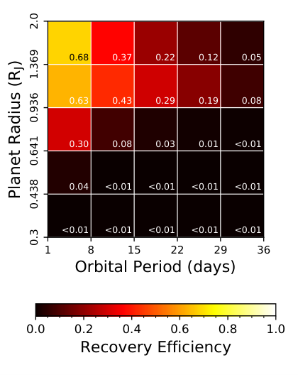
Figure 5 shows the recovery efficiency of our injected transits across our radius and period bins. We define recovery efficiency as the fraction of transits that were successfully recovered, and in Figure 5, this is the efficiency across all of the injected transits and all of the stars. As would be expected, the recovery efficiency trends towards higher values for larger planets and smaller orbital periods. Of note, though, is that for period bins greater than 8 days, the recovery efficiency is higher for our second-largest planet radius bin (0.9 to 1.4 RJ) than for our largest planet radius bin (1.4–2 RJ). A possible explanation for this is that the deeper transits produced by the larger radius planets were more likely to be distorted and diminished by our photometric processing pipeline than the shallower transits from 0.9–1.4 RJ planets. The shorter-duration transits at smaller periods may be less likely to be impacted by the processing pipeline, which would explain the higher recovery efficiency seen for the larger planets for periods shorter than eight days. Also, we found that some of the deepest transits had the bottom portions of the transits trimmed by the sigma clipping. Such transits were still detectable by BLS but had a lower S/PN due to the diminished apparent transit depth.
Figure 6 shows the recovery efficiency broken down by magnitude, orbital period, and planet radius. We see (as expected) that shorter-period planets have a higher recovery efficiency than longer-period planets. We also see lower recovery efficiencies for the brightest stars relative to the peak efficiencies reached (usually around –17). This is due to the large radii of the brightest stars (see top axis of Figure 6) diminishing the transit depth and thus the signal size and recoverability. In the leftmost panel of Figure 6, corresponding to the largest-radius injected planets, we also note that detection efficiencies tend to be higher at both and than at , particularly in the 1–15 day period range. The non-monotonic variation in detection efficiency with magnitude is due to the different magnitude dependencies of two competing effects. Brighter stars in the cluster have higher precision light curves, which tend to increase the signal to noise of the transits. However, fainter stars in the cluster have smaller stellar radii, which leads to deeper transits for a given planetary radius. In the middle and rightmost panels of Figure 6, this increase in recovery efficiency at the faintest magnitudes is not seen. In the rightmost panel, we see a large drop in recovery efficiency overall for 0.64–0.94 RJ planets relative to the other two panels—the larger radii planets.
IV.2 Planet Occurrence Rates and Limits
We now present our calculated occurrence rate limits and compare with other published occurrence rates. Figure 7 shows the calculated occurrence rate upper limits across our radius–period bins, and in the case of the bin containing our single S/PN planet candidate (W2282), the range for the occurrence rate if the planet candidate is real. For our shortest period bins, we are able to get down to limits of 1.6–3.5% for bins with planet radius larger than 0.64 RJ. To put these limits in context, Table 3 compares our occurrence rate limits with those of works using Kepler, TESS, or RV surveys for field stars. These previous works are: Kepler-based occurrence rates from Howard et al. 2012, Fressin et al. 2013, Masuda & Winn 2017, and Petigura et al. 2018; a TESS-based occurrence rate from Zhou et al. 2019; and RV occurrence rates from Mayor et al. 2011 and Wright et al. 2012. Table 4 compares our occurrence rate limits with those of previous GC planet searches: Gilliland et al. 2000 and Weldrake et al. 2005 for 47 Tuc, Weldrake et al. 2008 for Cen, and Nascimbeni et al. 2012 for NGC 6397.
| Per. RangeaaThe period range used in the comparison work for the occurrence rate calculation. Note that the smallest period used in this work is 1 day and so our calculation truncates smaller period ranges at 1 day. | Rad. RangebbThe planet radius range used in the comparison work for the occurrence rate calculation. Several references used R⊕ as their unit of radius and these values have been converted to RJ and rounded. Note that the largest radius examined in this work is 2 RJ and so our calculation truncates larger radius ranges at 2 RJ. | Reference | Published RateccThe comparison work’s planet occurrence rate as published. | Our Upper LimitddOur calculated occurrence rate upper limit for the same period and radius range. | Our RateeeOur calculated occurrence rate assuming W2282 is a planet. This value is not included if W2282 does not fall in the given period and radius ranges. |
|---|---|---|---|---|---|
| (day) | (RJ) | ||||
| Kepler Studies | |||||
| 0.8–10 | 0.71–2.85 | Howard et al. 2012 | % | % | 0.38–3.3% |
| 0.8–50ffOur calculation truncates at 36 days. | 0.71–2.85 | Howard et al. 2012 | % | % | 1.1–9.1% |
| 0.8–10 | 0.36–0.71 | Howard et al. 2012 | % | % | … |
| 0.8–10 | 0.54–1.96 | Fressin et al. 2013 | % | % | 0.44–3.9% |
| 0.8–17 | 0.54–1.96 | Fressin et al. 2013 | % | % | 0.66–5.7% |
| 0.8–29 | 0.54–1.96 | Fressin et al. 2013 | % | % | 1.0–8.9% |
| 0–10 | 0.8–2 | Masuda & Winn 2017 | % | % | 0.36–3.2% |
| 0–10 | 0.8–2 | Masuda & Winn 2017 | %ggFor this value, Masuda & Winn 2017 restricted their analysis to the Kepler stars that were in the same range of masses as the stars search in 47 Tuc for planets by Gilliland et al. 2000. | % | 0.36–3.2% |
| 1–10 | 0.71–2.14 | Petigura et al. 2018 | % | % | 0.38–3.3% |
| TESS Study | |||||
| 0.9–10 | 0.8–2.5 | Zhou et al. 2019 | % | % | 0.36–3.2% |
| RV Studies | |||||
| 0–11 | 0.72–2hhThese were limits in mass rather than radius. We converted the lower mass limit to a radius using the empirical relation derived by Chen & Kipping 2017 and imposed our default upper limit of 2 RJ. | Mayor et al. 2011 | % | % | 0.40–3.5% |
| 0–10 | 0.55–2hhThese were limits in mass rather than radius. We converted the lower mass limit to a radius using the empirical relation derived by Chen & Kipping 2017 and imposed our default upper limit of 2 RJ. | Wright et al. 2012 | % | % | 0.44–3.8% |
| Per. RangeaaThe period range used in the comparison work for the occurrence rate calculation. | Rad. RangebbThe planet radius range used in the comparison work for the occurrence rate calculation. The radius ranges used were not always clear in the comparison works, so we made our best guess, taking into account our radius–period grid boundaries. Note that the largest radius examined in this work is 2 RJ and so our calculation truncates larger radius ranges at 2 RJ. | Reference | Published RateccThe comparison work’s planet occurrence rate upper limit as published. | Our Upper LimitddOur calculated occurrence rate upper limit for the same period and radius range. | Our RateeeOur calculated occurrence rate assuming W2282 is a planet. This value is not included if W2282 does not fall in the given period and radius ranges. |
|---|---|---|---|---|---|
| (day) | (RJ) | ||||
| 1–8 | 0.64–2 | Gilliland et al. 2000ffProvided courtesy K. Masuda (private communication) based on the work in Masuda & Winn 2017. The calculated 3 occurrence rate upper limit is based on the same stellar mass range described in Table 3, note g. | % | % | 0.35–3.1% |
| 1–16 | 1–2 | Weldrake et al. 2005 | … | % | % |
| 1–5ggThe published rate is for their 1–5 day calculation; we performed our calculation over 1–8 days to guarantee at least one of our radius–period bins be included. Similarly, the quoted rate is only for RJ objects, but we had to use 1.37–2 RJ objects to cover a whole bin. | 1.5–2ggThe published rate is for their 1–5 day calculation; we performed our calculation over 1–8 days to guarantee at least one of our radius–period bins be included. Similarly, the quoted rate is only for RJ objects, but we had to use 1.37–2 RJ objects to cover a whole bin. | Weldrake et al. 2008 | % | %hh95% confidence instead of our typical 3, to match the confidence level used by both Weldrake et al. 2008 and Nascimbeni et al. 2012. | … |
| 1–14iiThe upper end of the period range was arrived at dividing their total observation duration (28 days) in half; planet radius range chosen to span their single injected planet radius, 1 RJ. | 0.94–1.37iiThe upper end of the period range was arrived at dividing their total observation duration (28 days) in half; planet radius range chosen to span their single injected planet radius, 1 RJ. | Nascimbeni et al. 2012 | % | %hh95% confidence instead of our typical 3, to match the confidence level used by both Weldrake et al. 2008 and Nascimbeni et al. 2012. | 0.31–1.7% |
As seen in Table 3, in no case were we able to set an upper limit that shows an occurrence rate smaller than what we would expect from the field population. And even if W2282 or a comparable planet candidate in the HJ regime is shown to actually be a planet, most of the Kepler- or TESS-based occurrence rates would be consistent with the lower end of our calculated occurrence rate ranges, though the upper ends of our ranges are inconsistent in all those cases. Thus based on these previous studies, and ignoring the metallicity dependence of HJ occurrence as seen in the field, we would expect to have a non-vanishing probability of finding a planet. Comparing with the RV studies, the RV rates fall within our W2282-based occurrence rate ranges, also suggesting from these results that there is some meaningful, if small, probability of finding a planet.
Comparing with the previous searches in GCs, and focusing first on the 47 Tuc surveys as those were the most constraining, Masuda & Winn 2017 showed that Gilliland et al. 2000 should have found planets in their survey, and that Weldrake et al. 2005 should also have found 2 planets in their survey. Thus their results (possibly) show a lower occurrence rate in 47 Tuc than found by Kepler for the field population for the period ranges searched. Our results do not reach such a constraining level for HJs. However, our sensitivity reaches further in planet radius and period than either of those two previous surveys. Our 78 day baseline and the nearly continuous nature of the observations would virtually guarantee us three visible transits for orbital periods up to 26 days and for some cases out to 39 days. This is compared to the 8.3 day baseline of Gilliland et al. 2000 and the 33 day baseline of Weldrake et al. 2005. Additionally, Gilliland et al. 2000 were insensitive to nearly all planets with a radius below 0.8 RJ and had at best 40% recovery of 1 RJ objects for the optimal stellar magnitude. Our work is still reasonably sensitive down to 0.6 RJ for small periods and somewhat sensitive down to 0.4 RJ.
In Table 4, we do have a more constraining upper limit than the work in Cen by Weldrake et al. 2008 for their very limited period and radius range. We also improve on the limit determined by Nascimbeni et al. 2012. They were able to put a (95% confidence) upper limit of 9.1% on the occurrence of 1 RJ objects with periods between 1 and 14 days, while we are able to put an upper limit of 0.93% for the same period range and a similar planet radius range at the same confidence level. Weldrake et al. 2005 did not provide any quantification of their sensitivity to planet radius, but their calculations assumed a relatively large radius of 1.3 RJ, and we assume they were sensitive to planets of that radius and larger.
The primary contribution of this work is the new parameter range it explores for planet occurrence rates in GCs, in both planet radius and orbital period. The occurrence rate limits in these new parameter ranges ( RJ at short periods and days for large-radius planets) are shown in Table 3 in comparison with the field occurrence rates. In particular, we set occurrence rate upper limits of 16% for 0.36–0.71 RJ planets with 1–10 day periods and 6.1% for 0.71–2 RJ planets with 1–36 day periods. While these numbers may not seem impressive when compared to the equivalent occurrence rates determined from Kepler (% for 0.36–0.71 RJ planets with 0.8–10 day periods and % for 0.71–2 RJ planets with 1–50 day periods; Howard et al. 2012), these are the first limits set for planets in a GC in these period and radius regimes. These limits demonstrate that the occurrence of planets in M4 just outside the HJ regime (in terms of period or radius) is not ubiquitous, and, for the 0.71–2 RJ, 1–36 day range, is at most a factor of about five higher than has been found for the field population.
V Discussion
This work represents the first look at a planet occurrence rate for the GC M4, and the fifth photometry-based examination of a planet occurrence rate for a GC. It is worth noting that, although our results do not place very stringent constraints on the occurrence of planets in M4, Kepler was not designed or optimized for looking at GCs—in particular, the 4″/pixel image resolution led to significant blending in the images—and the superstamp observations of M4 were originally intended for observing RR Lyrae variables. Obtaining even the level of constraints we did from a telescope and observations not originally intended for a GC planet search is yet another demonstration of an unanticipated scientific result from Kepler.
Though our constraints cannot rule out planet occurrence rates for M4 matching those of the field stars, given the current uncertainties on planet formation—particularly the formation of close-in giant planets—and uncertainties on GC formation, obtaining any constraints on planet occurrence in GCs for new regimes of planet radius and period is useful. It may be that the occurrence of certain kinds of close-in planets in GCs is more common due to some unique aspect of GCs.
There are some reasons we might expect the occurrence of close-in planets to be higher in a GC than in the field. For example, Hamers & Tremaine 2017 demonstrated that the increased number of close stellar encounters experienced by GC stars over their lifetimes could enhance the HJ occurrence rate for certain stellar densities (peak formation occurred at a density of pc-3) if HJs are formed through high-eccentricity migration. The formation of GCs themselves is still something of a mystery (see Gratton et al. 2012 for a review), and perhaps there is something unique about the formation of stars in GCs that would increase the formation of close-in planets. Our results, with those of the previous GC planet occurrence works, provide constraints on just how enhanced a planet occurrence rate might be should there indeed be enhanced close-in planet formation in GCs.
On the other hand, much work has been done to show why specifically HJ occurrence in GCs might be suppressed. The occurrence of HJs is known to correlate with host star metallicity (e.g., Fischer & Valenti 2005) and this has been used to argue that the low metallicities of GCs would inhibit HJ formation (for example, Santos et al. 2001 showed the known metallicity dependence as being able to explain the 47 Tuc planet non-detection of Gilliland et al.), but the reason behind a metallicity–occurrence connection is not well understood and it may be that the underlying cause of this connection does not apply in the unique environments of GCs. Additionally, the dense stellar environment of GCs and the associated levels of radiation from particularly the nearby massive stars may inhibit giant-planet formation (Armitage 2000; Adams et al. 2004; Thompson 2013). Also, in addition to enhancing the rate of close-in planets, dynamical interactions with passing stars can also remove planets from planetary systems (Sigurdsson 1992; Davies & Sigurdsson 2001; Bonnell et al. 2001; Fregeau et al. 2006; Spurzem et al. 2009), particularly planets on wide orbits. Interactions between stars and protoplanetary disks lead to decreases in disk sizes as well (Breslau et al. 2014). Until better constraints or actual occurrence rates are determined for GCs, for a larger range of planet radii and orbital periods than are presently accessible from existing data, it will be difficult to determine the precise impact a GC environment has on planet formation and occurrence.

As an analysis of how an improvement on our light curves and/or noise characterization and removal could improve our occurrence rate limits, we show a forecast in Figure 8 of the limits that would be set if an S/PN threshold of eight could be imposed instead of 12 and assuming no planets were found. W2282 and the associated occurrence rate is still included for comparison with Figure 7. Our upper limits in the HJ regime would not improve by very much, but we would be able to place more stringent constraints for across all the periods examined, and for for the shortest periods examined here. Even if our limits in the HJ regime do not improve much, a better understanding of the noise would allow for an improved vetting of the current planet candidates.
As limited as our constraints are, they may be the best to come for a while. The only near-term continuous photometric survey is TESS, but with its 20″/pixel image resolution it will leave most of the stars in GCs hopelessly blended. Moreover, the 1 month observation span most of its survey field will be covered by is only about a third the span of what is available in this work with K2. An HST campaign similar to that of Gilliland et al. 2000 for M4—being about half the distance as 47 Tuc—should permit a factor of two increase in the signal-to-noise ratio for stars of comparable masses and evolutionary state as in 47 Tuc; a campaign along these lines might be considered. The main limiting factor in setting the HJ occurrence limit from the K2 data is the relatively small number of cluster stars observed, (4000 compared to 34,000 GC stars in Gilliland et al. 2000 and 20,000 GC stars in Weldrake et al. 2005). The K2 superstamp covered a relatively small fraction of the stars in the cluster, so a survey that covers more of the cluster could be useful.
Despite the low S/PN of our planet candidates, given the scientific impact of discovering and characterizing a transiting planet in a GC, we argue that it is worth the effort to confirm whether these are real planet signals.
Unfortunately, the data are already five years old. Referencing Table 2, the transit timing uncertainties for W2863 (0.67 days) and W1184 (0.28 days) are considerable. Taking the number of transits that are expected to have occurred in the last five years and multiplying by the period uncertainties as an approximate calculation of additional uncertainty on transit timing arising from the period uncertainties, we get: W2282, 2.0 days; W2863, 54 days; W74, 5.5 days; W1955, 1.0 days; W3055, 0.45 days; W1184, 23 days; and W3128, 16 days. Thus only for W74, W1955, and W3055 would the transit epoch number be known with certainty if a transit were to be observed five years on. In no case is the present transit timing known with sufficient precision to be sure of catching a transit in one night’s observation, so an extended follow-up campaign would be needed. In this the crowded nature of the cluster and the manageably sized field of view of the K2 superstamp (10′ by 20′) are advantages. Many available wide field imagers can cover a large fraction of or even the entire superstamp, allowing for simultaneous observation of more than one planet candidate, and the data would also have the advantage of observing other interesting variables guaranteed to be present (see Wallace et al. 2019a for a catalog).
VI Conclusion
We searched for transiting planets in the GC M4 using data from the K2 mission. These data represent the longest continuous observation of a GC, permitting a search for the longest-period planets ever searched in a GC. The data are also of sufficient quality to be sensitive to planets of smaller radii than any previous transit search in a GC. From 3784 light curves extracted from the data, with a maximum observation duration of 78 days, and using a BLS transit search followed by a by-eye vetting, we identified 27 planet candidates in the data. An analysis of the systematic noise in the light curves revealed that a S/PN cutoff value of 12 should be used to remove probable false positives, with only one of the planet candidates exceeding this cutoff value, yet there still remains uncertainty as to whether this might be a false alarm. Despite this, information on this and six other of our most promising candidates are presented. The light curves are publicly available at Wallace et al. 2019b.
We calculated 3 occurrence rate upper limits based on a non-detection of planets and occurrence rate ranges assuming our S/PN planet candidate as real, for a variety of period and planet radius ranges. Comparing these limits and rates to the literature, for previous GC works, we find a factor of two lower occurrence rate limit than was calculated by Weldrake et al. 2008 for Cen for R RJ objects. We also improve on the Nascimbeni et al. 2012 limit for 1 RJ planets with day orbits, obtaining a 2 limit of %. Our limit for a similar period and radius range as the landmark study of Gilliland et al. 2000 was sensitive to, 1–8 days and 0.64–2 RJ, was %, compared to the % limit determined by Masuda & Winn 2017 using the Gilliland et al. 2000 data. Comparing with occurrence rates calculated from field star transit surveys, our HJ occurrence rate limits are factors of about four to six larger than the Kepler and TESS rates. Similarly, for RV studies, our HJ occurrence limits are about a factor of two higher than the rate of Wright et al. 2012 and about a factor of three higher than the rate of Mayor et al. 2011. Our rate upper limits for longer period orbits ( days) of 1 RJ objects and for smaller planets (0.4 RJ and larger) are much larger than the rates known for those regimes from Kepler and are not very constraining, but are the first such limits ever set for a GC.
Future work that could be done to build off these results includes photometric follow up of the planet candidates to confirm the transits and improving the systematic noise characterization and abatement in the light curves to permit greater sensitivity to lower S/PN transits. Lowering the S/PN threshold would allow us to put significantly better constraints on day planets with RJ planets and for RJ planets across all periods examined.
References
- Adams et al. (2004) Adams, F. C., Hollenbach, D., Laughlin, G., & Gorti, U. 2004, ApJ, 611, 360, doi: 10.1086/421989
- Alard & Lupton (1998) Alard, C., & Lupton, R. H. 1998, ApJ, 503, 325, doi: 10.1086/305984
- Armitage (2000) Armitage, P. J. 2000, A&A, 362, 968. https://arxiv.org/abs/astro-ph/0007044
- Arzoumanian et al. (1996) Arzoumanian, Z., Joshi, K., Rasio, F. A., & Thorsett, S. E. 1996, International Astronomical Union Colloquium, 160, 525–530, doi: 10.1017/S0252921100042287
- Astropy Collaboration et al. (2018) Astropy Collaboration, Price-Whelan, A. M., Sipőcz, B. M., et al. 2018, AJ, 156, 123, doi: 10.3847/1538-3881/aabc4f
- Backer et al. (1993) Backer, D. C., Foster, R. S., & Sallmen, S. 1993, Nature, 365, 817, doi: 10.1038/365817a0
- Barentsen (2016) Barentsen, G. 2016, barentsen/k2mosaic: v2.0.0, Zenodo, doi: 10.5281/zenodo.167343. https://zenodo.org/record/167343#.W9nI15y1thE
- Beer et al. (2004) Beer, M. E., King, A. R., & Pringle, J. E. 2004, MNRAS, 355, 1244, doi: 10.1111/j.1365-2966.2004.08404.x
- Bhatti et al. (2017) Bhatti, W., Bouma, L. G., & Wallace, J. 2017, astrobase, Zenodo, doi: 10.5281/zenodo.1011188. https://doi.org/10.5281/zenodo.1011188
- Bonnell et al. (2001) Bonnell, I. A., Smith, K. W., Davies, M. B., & Horne, K. 2001, MNRAS, 322, 859, doi: 10.1046/j.1365-8711.2001.04171.x
- Braga et al. (2015) Braga, V., Dall’Ora, M., Bono, G., et al. 2015, ApJ, 799, 165
- Breslau et al. (2014) Breslau, A., Steinhausen, M., Vincke, K., & Pfalzner, S. 2014, A&A, 565, A130, doi: 10.1051/0004-6361/201323043
- Chen & Kipping (2017) Chen, J., & Kipping, D. 2017, ApJ, 834, 17, doi: 10.3847/1538-4357/834/1/17
- Claret (2018) Claret, A. 2018, A&A, 618, A20, doi: 10.1051/0004-6361/201833060
- Davies & Sigurdsson (2001) Davies, M. B., & Sigurdsson, S. 2001, MNRAS, 324, 612, doi: 10.1046/j.1365-8711.2001.04336.x
- Ercolano & Clarke (2010) Ercolano, B., & Clarke, C. J. 2010, MNRAS, 402, 2735, doi: 10.1111/j.1365-2966.2009.16094.x
- Fischer & Valenti (2005) Fischer, D. A., & Valenti, J. 2005, ApJ, 622, 1102, doi: 10.1086/428383
- Ford et al. (2000) Ford, E. B., Joshi, K. J., Rasio, F. A., & Zbarsky, B. 2000, ApJ, 528, 336, doi: 10.1086/308167
- Ford et al. (2008) Ford, E. B., Quinn, S. N., & Veras, D. 2008, The Astrophysical Journal, 678, 1407, doi: 10.1086/587046
- Fregeau et al. (2006) Fregeau, J. M., Chatterjee, S., & Rasio, F. A. 2006, ApJ, 640, 1086, doi: 10.1086/500111
- Fressin et al. (2013) Fressin, F., Torres, G., Charbonneau, D., et al. 2013, ApJ, 766, 81, doi: 10.1088/0004-637X/766/2/81
- Gaia Collaboration et al. (2016a) Gaia Collaboration, Brown, A. G. A., Vallenari, A., et al. 2016a, A&A, 595, A2, doi: 10.1051/0004-6361/201629512
- Gaia Collaboration et al. (2016b) Gaia Collaboration, Prusti, T., de Bruijne, J. H. J., et al. 2016b, A&A, 595, A1, doi: 10.1051/0004-6361/201629272
- Gaia Collaboration et al. (2018) Gaia Collaboration, Brown, A. G. A., Vallenari, A., et al. 2018, A&A, 616, A1, doi: 10.1051/0004-6361/201833051
- Gilliland et al. (2000) Gilliland, R. L., Brown, T. M., Guhathakurta, P., et al. 2000, ApJ, 545, L47, doi: 10.1086/317334
- Gratton et al. (2012) Gratton, R. G., Carretta, E., & Bragaglia, A. 2012, A&A Rev., 20, 50, doi: 10.1007/s00159-012-0050-3
- Hamers & Tremaine (2017) Hamers, A. S., & Tremaine, S. 2017, AJ, 154, 272, doi: 10.3847/1538-3881/aa9926
- Harris (1996) Harris, W. E. 1996, AJ, 112, 1487
- Hartman & Bakos (2016) Hartman, J. D., & Bakos, G. Á. 2016, Astronomy and Computing, 17, 1, doi: 10.1016/j.ascom.2016.05.006
- Hendricks et al. (2012) Hendricks, B., Stetson, P. B., VandenBerg, D. A., & Dall’Ora, M. 2012, AJ, 144, 25, doi: 10.1088/0004-6256/144/1/25
- Howard et al. (2012) Howard, A. W., Marcy, G. W., Bryson, S. T., et al. 2012, ApJS, 201, 15, doi: 10.1088/0067-0049/201/2/15
- Howell et al. (2014) Howell, S. B., Sobeck, C., Haas, M., et al. 2014, PASP, 126, 398, doi: 10.1086/676406
- Hunter (2007) Hunter, J. D. 2007, Computing In Science & Engineering, 9, 90
- Husser et al. (2013) Husser, T. O., Wende-von Berg, S., Dreizler, S., et al. 2013, A&A, 553, A6, doi: 10.1051/0004-6361/201219058
- Ida & Lin (2004) Ida, S., & Lin, D. N. C. 2004, ApJ, 616, 567, doi: 10.1086/424830
- Johansen et al. (2009) Johansen, A., Youdin, A., & Mac Low, M.-M. 2009, ApJ, 704, L75, doi: 10.1088/0004-637X/704/2/L75
- Johnson et al. (2010) Johnson, J. A., Aller, K. M., Howard, A. W., & Crepp, J. R. 2010, PASP, 122, 905, doi: 10.1086/655775
- Johnson & Li (2012) Johnson, J. L., & Li, H. 2012, ApJ, 751, 81
- Jones et al. (2001) Jones, E., Oliphant, T., Peterson, P., et al. 2001, SciPy: Open source scientific tools for Python. http://www.scipy.org/
- Kaluzny et al. (2013) Kaluzny, J., Thompson, I. B., Rozyczka, M., et al. 2013, AJ, 145, 43, doi: 10.1088/0004-6256/145/2/43
- Kipping (2013) Kipping, D. M. 2013, MNRAS, 434, L51, doi: 10.1093/mnrasl/slt075
- Kovács et al. (2005) Kovács, G., Bakos, G., & Noyes, R. W. 2005, MNRAS, 356, 557, doi: 10.1111/j.1365-2966.2004.08479.x
- Kovács et al. (2002) Kovács, G., Zucker, S., & Mazeh, T. 2002, A&A, 391, 369, doi: 10.1051/0004-6361:20020802
- Lindegren et al. (2018) Lindegren, L., Hernández, J., Bombrun, A., et al. 2018, A&A, 616, A2, doi: 10.1051/0004-6361/201832727
- Lomb (1976) Lomb, N. R. 1976, Ap&SS, 39, 447, doi: 10.1007/BF00648343
- Maíz Apellániz & Weiler (2018) Maíz Apellániz, J., & Weiler, M. 2018, A&A, 619, A180, doi: 10.1051/0004-6361/201834051
- Mandel & Agol (2002) Mandel, K., & Agol, E. 2002, ApJ, 580, L171, doi: 10.1086/345520
- Marigo et al. (2017) Marigo, P., Girardi, L., Bressan, A., et al. 2017, ApJ, 835, 77, doi: 10.3847/1538-4357/835/1/77
- Masuda & Hotokezaka (2018) Masuda, K., & Hotokezaka, K. 2018, arXiv e-prints, arXiv:1808.10856. https://arxiv.org/abs/1808.10856
- Masuda & Winn (2017) Masuda, K., & Winn, J. N. 2017, AJ, 153, 187, doi: 10.3847/1538-3881/aa647c
- Mayor et al. (2011) Mayor, M., Marmier, M., Lovis, C., et al. 2011, arXiv e-prints, arXiv:1109.2497. https://arxiv.org/abs/1109.2497
- McWilliam & Bernstein (2008) McWilliam, A., & Bernstein, R. A. 2008, ApJ, 684, 326, doi: 10.1086/589957
- Michel (1994) Michel, F. C. 1994, ApJ, 432, 239, doi: 10.1086/174565
- Mochejska et al. (2002) Mochejska, B. J., Kaluzny, J., Thompson, I., & Pych, W. 2002, AJ, 124, 1486, doi: 10.1086/342015
- Nascimbeni et al. (2012) Nascimbeni, V., Bedin, L. R., Piotto, G., De Marchi, F., & Rich, R. M. 2012, A&A, 541, A144, doi: 10.1051/0004-6361/201118655
- Neeley et al. (2015) Neeley, J., Marengo, M., Bono, G., et al. 2015, The Astrophysical Journal, 808, 11
- Ochsenbein et al. (2000) Ochsenbein, F., Bauer, P., & Marcout, J. 2000, A&AS, 143, 23, doi: 10.1051/aas:2000169
- Oliphant (2006) Oliphant, T. 2006, Guide to NumPy (Trelgol Publishing). http://www.tramy.us/numpybook.pdf
- Pál (2012) Pál, A. 2012, MNRAS, 421, 1825, doi: 10.1111/j.1365-2966.2011.19813.x
- Pedregosa et al. (2011) Pedregosa, F., Varoquaux, G., Gramfort, A., et al. 2011, Journal of Machine Learning Research, 12, 2825
- Penev et al. (2018) Penev, K., Bouma, L. G., Winn, J. N., & Hartman, J. D. 2018, The Astronomical Journal, 155, 165, doi: 10.3847/1538-3881/aaaf71
- Petigura et al. (2018) Petigura, E. A., Marcy, G. W., Winn, J. N., et al. 2018, AJ, 155, 89, doi: 10.3847/1538-3881/aaa54c
- Pont et al. (2006) Pont, F., Zucker, S., & Queloz, D. 2006, MNRAS, 373, 231, doi: 10.1111/j.1365-2966.2006.11012.x
- Rasio (1994) Rasio, F. A. 1994, ApJ, 427, L107, doi: 10.1086/187376
- Richer et al. (2003) Richer, H. B., Ibata, R., Fahlman, G. G., & Huber, M. 2003, ApJ, 597, L45, doi: 10.1086/379800
- Riello et al. (2018) Riello, M., De Angeli, F., Evans, D. W., et al. 2018, A&A, 616, A3, doi: 10.1051/0004-6361/201832712
- Santos et al. (2001) Santos, N. C., Israelian, G., & Mayor, M. 2001, A&A, 373, 1019, doi: 10.1051/0004-6361:20010648
- Scargle (1982) Scargle, J. D. 1982, ApJ, 263, 835, doi: 10.1086/160554
- Sigurdsson (1992) Sigurdsson, S. 1992, ApJ, 399, L95, doi: 10.1086/186615
- Sigurdsson et al. (2003) Sigurdsson, S., Richer, H. B., Hansen, B. M., Stairs, I. H., & Thorsett, S. E. 2003, Science, 301, 193, doi: 10.1126/science.1086326
- Soares-Furtado et al. (2017) Soares-Furtado, M., Hartman, J. D., Bakos, G. Á., et al. 2017, PASP, 129, 044501, doi: 10.1088/1538-3873/aa5c7c
- Spurzem et al. (2009) Spurzem, R., Giersz, M., Heggie, D. C., & Lin, D. N. C. 2009, ApJ, 697, 458, doi: 10.1088/0004-637X/697/1/458
- Thompson (2013) Thompson, T. A. 2013, MNRAS, 431, 63, doi: 10.1093/mnras/stt102
- Thorsett et al. (1999) Thorsett, S. E., Arzoumanian, Z., Camilo, F., & Lyne, A. G. 1999, ApJ, 523, 763, doi: 10.1086/307771
- Thorsett et al. (1993) Thorsett, S. E., Arzoumanian, Z., & Taylor, J. H. 1993, ApJ, 412, L33, doi: 10.1086/186933
- Vanderburg & Johnson (2014) Vanderburg, A., & Johnson, J. A. 2014, PASP, 126, 948, doi: 10.1086/678764
- Vanderburg et al. (2016) Vanderburg, A., Latham, D. W., Buchhave, L. A., et al. 2016, ApJS, 222, 14
- Wallace (2018) Wallace, J. J. 2018, Research Notes of the AAS, 2, 213
- Wallace et al. (2019a) Wallace, J. J., Hartman, J. D., Bakos, G. A., & Bhatti, W. 2019a, arXiv e-prints, arXiv:1908.02373. https://arxiv.org/abs/1908.02373
- Wallace et al. (2019b) Wallace, J. J., Hartman, J. D., Bakos, G. Á., & Bhatti, W. 2019b, Light Curves from a Search for Variable Stars in the Globular Cluster M4 with K2, DataSpace at Princeton University. http://arks.princeton.edu/ark:/88435/dsp01h415pd368
- Weldrake et al. (2008) Weldrake, D. T. F., Sackett, P. D., & Bridges, T. J. 2008, ApJ, 674, 1117, doi: 10.1086/524917
- Weldrake et al. (2005) Weldrake, D. T. F., Sackett, P. D., Bridges, T. J., & Freeman, K. C. 2005, ApJ, 620, 1043, doi: 10.1086/427258
- Wenger et al. (2000) Wenger, M., Ochsenbein, F., Egret, D., et al. 2000, A&AS, 143, 9, doi: 10.1051/aas:2000332
- Wright et al. (2012) Wright, J. T., Marcy, G. W., Howard, A. W., et al. 2012, ApJ, 753, 160, doi: 10.1088/0004-637X/753/2/160
- Yi et al. (2001) Yi, S., Demarque, P., Kim, Y.-C., et al. 2001, ApJS, 136, 417, doi: 10.1086/321795
- Zhou et al. (2019) Zhou, G., Huang, C. X., Bakos, G. Á., et al. 2019, arXiv e-prints, arXiv:1906.00462. https://arxiv.org/abs/1906.00462