Iterated Type Partitions

G. Cordasco Affiliation: University of Campania “L.Vanvitelli”, Italy L. Gargano Affiliation: University of Salerno, Italy A. A. Rescigno Affiliation: University of Salerno, Italy

Abstract

This paper deals with the complexity of some natural graph problems when parametrized by measures that are restrictions of clique-width, such as modular-width and neighborhood diversity. The main contribution of this paper is to introduce a novel parameter, called iterated type partition, that can be computed in polynomial time and nicely places between modular-width and neighborhood diversity. We prove that the Equitable Coloring problem is W[1]-hard when parametrized by the iterated type partition. This result extends to modular-width, answering an open question about the possibility to have FPT algorithms for Equitable Coloring when parametrized by modular-width. On the contrary, we show that the Equitable Coloring problem is instead FPT when parameterized by neighborhood diversity. Furthermore, we present simple and fast FPT algorithms parameterized by iterated type partition that provide optimal solutions for several graph problems; in particular this paper presents algorithms for the Dominating Set, the Vertex Coloring and the Vertex Cover problems. While the above problems are already known to be FPT with respect to modular-width, the novel algorithms are both simpler and more efficient: For the Dominating set and Vertex Cover problems, our algorithms output an optimal set in time $O(2^{t}+poly(n))$ , while for the Vertex Coloring problem, our algorithm outputs an optimal set in time $O(t^{2.5t+o(t)}\log n+poly(n))$ , where $n$ and $t$ are the size and the iterated type partition of the input graph, respectively.

keywords: Parameterized Complexity, Fixed-parameter tractable algorithms, W[1]-hardness, Neighborhood Diversity, Modular-width.

1 Introduction

Some NP-hard problems can be solved by algorithms that are exponential only in the size of a fixed parameter while they are polynomial in the size of the input. Such problems are called fixed-parameter tractable, because the problem can be solved efficiently for small values of the parameter [9, 32]. Formally, a parameterized problem with input size $n$ and parameter ${{t}}$ is called fixed parameter tractable (FPT) if it can be solved in time $f({{t}})\cdot n^{c}$ , where $f$ is a function only depending on ${{t}}$ and $c$ is a constant.

An important quality of a parameter is that is is easy to compute. Unfortunately there are several parameters whose computation is an NP-hard problem. As an example computing treewidth, rankwidth, and vertex cover are all NP-hard problems but they are computable in FPT time when their respective parameters are bounded; moreover, the parameterized complexity of computing the clique-width of a graph exactly is still an open problem [10].

We start from two recently introduced parameters: modular-width [20] and neighborhood diversity [30]. Both parameters received much attention [1, 2, 5, 6, 11, 17, 19, 22, 23, 25] also due to their property of being computable in polynomial time [20, 30].

As the main contribution of this paper we introduce a novel parameter called Iterated Type Partition, which nicely places between the two above parameters and allows to obtain new algorithms and hardness results.

1.1 Modular-width

The notion of modular decomposition of graphs was introduced by Gallai in [21], as a tool to define hierarchical decompositions of graphs. It has been recently considered in [20] to define the modular-width parameter in the area of parameterized computation.

Consider graphs obtainable by an algebraic expression that uses the operations:

1)

Creation of an isolated vertex.
2)

Disjoint union of 2 graphs, i.e., the graph with vertex set $V(G_{1})\cup V(G_{2})$ and edge set $E(G_{1})\cup E(G_{2})$ .
3)

Complete join of 2 graphs, i.e., the graph with vertex set $V(G_{1})\cup V(G_{2})$ and edge set $E(G_{1})\cup E(G_{2})\cup\{(v,w)\ :\ v\in V(G_{1}),\ w\in V(G_{2})\}$ .
4)

Substitution operation $G(G_{1},\dots,G_{m})$ of the vertices $v_{1},\dots,v_{m}$ of $G$ by the modules $G_{1},\dots,G_{m}$ , i.e., the graph with vertex set $\bigcup_{1\leq\ell\leq m}V(G_{\ell})$ and edge set

$\bigcup_{1\leq\ell\leq m}E(G_{\ell})\cup\{(u,v)\ :\ u\in V(G_{i}),\ v\in V(G_{j}),\ (v_{i},v_{j})\in E(G)\}.$

As defined in [20], the modular-width of a graph $G$ , denoted $mw(G)$ , is the least integer $m$ such that $G$ can be obtained by using only the operations 1)–4) (in any number and order) and where each operation 4) has at most $m$ modules.

1.2 Neighborhood diversity

Given a graph $G=(V,E)$ , two nodes $u,v\in V$ have the same type iff $N(v)\setminus\{u\}=N(u)\setminus\{v\}$ . The neighborhood diversity of a graph $G$ , introduced by Lampis in [30] and denoted by nd $(G)$ , is the minimum number ${{t}}$ of sets in a partition $V_{1},V_{2},\ldots,V_{{t}}$ , of the node set $V$ , such that all the nodes in $V_{i}$ have the same type, for $i\in[t]$ ¹¹ 1 For a positive integer $n$ , we use $[n]$ to denote the set of the first $n$ integers, that is $[n]=\{1,2,\ldots,n\}$ ..
The family ${\cal V}=\{V_{1},V_{2},\ldots,V_{{t}}\}$ is called the type partition of $G$ .

Let $G=(V,E)$ be a graph with type partition ${\cal V}=\{V_{1},V_{2},\ldots,V_{{t}}\}$ . By definition, each $V_{i}$ induces either a clique or an independent set in $G$ . We treat singleton sets in the type partition as cliques. For each $V_{i},V_{j}\in{\cal V}$ , we get that either each node in $V_{i}$ is a neighbor of each node in $V_{j}$ or no node in $V_{i}$ has a neighbor in $V_{j}$ . Hence, between each pair $V_{i},V_{j}\in{\cal V}$ , there is either a complete bipartite graph or no edges at all.

Starting from a graph $G$ and its type partition ${\cal V}=\{V_{1},\ldots,V_{{t}}\}$ , we can see each element of ${\cal V}$ as a metavertex of a new graph $H$ , called the type graph of $G$ , with
- $V(H)=\{1,2,\cdots,{{t}}\}$
- $E(H)=\{(x,y)\ |\ x\neq y\mbox{ and for each $u\in V_{x}$, $v\in V_{y}$ it holds that $(u,v)\in E(G)$ }\}$ .
We say that $G$ is a base graph if it matches its type graph, that is, the type partition of $G$ consists of singletons, each representing a node in $V(G)$ , and $nd(G)=|V(G)|$ .

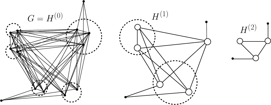
We introduce a new graph parameter, which generalizes neighborhood diversity. Given a graph $G$ , the Iterated Type Partition of $G$ is defined by iteratively constructing type graphs until a base graph is obtained.

Definition 1.

Given a graph $G=(V,E)$ , let ${H^{(0)}}=G$ and ${H^{(i)}}$ denote the type graph of ${H^{(i-1)}}$ , for $i\geq 1$ . Let $d$ be the smallest integer such that ${H^{(d)}}$ is a base graph. The iterated type partition of $G$ , denoted by ${itp}(G)$ , is the number of nodes of ${H^{(d)}}$ . The sequence of graphs ${H^{(0)}}=G,{H^{(1)}},\cdots,{H^{(d)}}$ is called the type graph sequence of $G$ and ${H^{(d)}}$ is denoted as the base graph of $G$ .

An example of a graph and its type graph sequence is given in Fig. 1.

Refer to caption — Figure 1: A graph $G$ with iterated type partition $5$ and its corresponding type graph sequence: $G=H^{(0)},H^{(1)},H^{(2)}.$ Dashed circles group nodes having the same type.

It is well-known that determining $nd(G)$ and the corresponding type partition, can be done in polynomial time [30]. As an immediate consequence, we have that

Theorem 1.

There exists a polynomial time algorithm, which given a graph $G=(V,E)$ , finds the type graphs sequence of $G$ and consequently the value $itp(G)$ .

1.3 Relation with other parameters

In this section we analyze the relations between the iterated type partition parameter and some other well known parameters.

We notice that, as an iteration of neighborhood diversity, the new parameter satisfies

itp(G)\leq nd(G).

(1)

Actually $itp(G)$ can be much smaller than $nd(G).$ Indeed consider the following:

•

Choose a positive integer $d$ and a connected base graph $H^{(d)}$ having $k$ nodes;
•
For $i=d,d-1,\ldots,1$ , a new graph $H^{(i-1)}$ is obtained as follows:
- –
  
  replace each node of $H^{(i)}$ , with an independent set of at least two nodes (if $d-i$ is even) or a clique of size at least two (if $d-i$ is odd).
- –
  
  for each edge of $H^{(i)}$ , put a complete bipartite graph between the nodes of the graphs that replace the endpoints of the edge.

The value $nd(H^{(0)})$ is the number of nodes in $H^{(1)}$ , that is at least $k2^{d-1}$ , while $itp(H^{(0)})$ is the size $k$ of $H^{(d)}$ .

We stress that iterated type partition is a “special case” of modular-width in which the modules in operation 4) can only be independent sets or cliques. Hence, it is not difficult to see that for every graph $G$

mw(G)\leq itp(G).

(2)

We know from [30] that $nd(G)\leq 2^{vc(G)}+vc(G)$ . Hence, by (1), we have $itp(G)\leq 2^{vc(G)}+vc(G)$ . Moreover, using the same arguments of [30] is it possible to show that $cw(G)\leq itp(G)+1.$ Finally, as for the neighborhood diversity we can easily show that the iterated type partition is incomparable to the treewidth by comparing the values of such parameters on a complete graph $K_{n}$ and a path on $n$ nodes. A summary of the relations holding between some popular parameters is given in Fig. 2. We refer to [16] for the formal definitions of treewidth and clique-width parameters.

1.4 Our results and related work

We give both tractability and hardness results for the new parameter.

The Equitable Coloring (EQC) problem. If the nodes of a graph $G$ are colored with $k$ colors such that no adjacent nodes receive the same color (i.e., properly colored) and the sizes of any two color classes differ by at most one, then $G$ is said to be equitably $k$ -colorable and the coloring is said an equitable $k$ -coloring. The goal is to minimize the number of used colors. The EQC problem is a well-studied problem, which has been analyzed in terms of parameterized positive or negative results with respect to many different parameters [24].

In particular, Fellows et al. [13] have shown that EQC problem parameterized by treewidth and number of colors is $W[1]$ -hard. A series of reductions proving that Equitable Coloring is $W[1]$ -hard for different subclasses of chordal graphs are given in [26]: The problem is shown to be W[1]-hard if parameterized by the number of colors for block graphs and for the disjoint union of split graphs; moreover, it remains W[1]-hard for $K_{1,4}$ -free interval graphs even when parameterized by treewidth, number of colors and maximum degree. In [3] an XP algorithm parameterized by treewidth is given. We notice that an XP algorithm for Equitable Coloring parametrized by iterated type partition can be obtained by using Theorem 17 in [28]. On the other side, Fiala et al. show that the Equitable Coloring problem is FPT when parameterized by the vertex cover number [15]. However, it was an open problem to establish the parameterized complexity of the Equitable Coloring problem parameterized by neigborhood diversity or modular-width. In section 2 we answer to these questions by proving the following results.

Theorem 2.

The Equitable Coloring problem is $W[1]$ -hard parametrized by itp.

Recalling (2), Theorem 2 immediately gives that the Equitable Coloring Problem is $W[1]$ -hard w.r.t. modular-width.

Theorem 3.

The EQC problem is $W[1]$ -hard parametrized by modular-width.

We also show that Equitable Coloring $W[1]$ -hardness drops when parameterized by the neighborhood diversity.

Theorem 4.

The EQC problem is FPT when parameterized by neighborhood diversity.

FPT algorithms w.r.t. itp. In the last section we deal with FPT algorithms with respect to iterated type partition. Some of the considered problems are already known to be FPT w.r.t modular-width. Nonetheless, we think that the new algorithms, parameterized by iterated type partition, are worthy to be considered, since they are much simpler, faster, and allow to easily determine not only the value, but also the optimal solution. As an example we consider here the dominating set (DS), the vertex coloring (Coloring), and the vertex cover (VC) problems.

Table 1 summarizes the contribution of this paper, in relation to known results.

	DS, VC	Coloring	EQC
$cw$	FPT[8]	W[1]-hard [16]	W[1]-hard [18]
$mw$	FPT[33]	FPT[20]	W[1]-hard [*]
$itp$	FPT( $O(2^{t}+poly(n))$ )[*]	FPT( $O(t^{2.5t+o(t)}\log n+poly(n))$ )[*]	W[1]-hard [*]
$nd$	FPT[30]	FPT[30]	FPT[*]
$vc$	FPT[30]	FPT[30]	FPT [15]

Table 1: The table summarizes the results known in literature for several problems parametrized by iterated type partition and related parameters.

t

denotes the value of the considered parameter and [*] denotes the result obtained in this paper.

2 Equitable coloring (EQC)

In this section we prove Theorems 2 and 4.

Equitable Coloring
Instance: A graph $G=(V,E)$ and an integer $k$ .
Question: Is it possible to color the nodes of $G$ with exactly $k$ colors in such a way that nodes connected by an edge receive different colors and each color class has either size $\lfloor|V|/k\rfloor$ or $\lceil|V|/k\rceil$ ?

2.1 Hardness

In order to prove that Equitable Coloring problem is $W[1]$ -hard if parameterized by iterated type partition, we present a reduction from the following Bin packing problem, which has been shown to be W[1]-hard when parameterized by the number of bins [27].

Bin-Packing
Instance: A collection of items $A=\{a_{1},a_{2},\cdots,a_{{{\ell}}}\}$ , a number $k$ of bins, and a bin capacity $B$ .
Question: $\exists$ a $k$ -partition ${{P}}_{1},\cdots,{{P}}_{k}$ of $A$ such that $\sum_{a_{j}\in{{P}}_{i}}a_{j}=B$ , $\forall\,i\in[k]$ ?

In general the Bin-Packing problem asks for the sum of the items of each bin to be at most $B$ ; however, the above version is equivalent to the general one (even from the parameterized point of view) as it is sufficient to add $kB-\sum_{j=1}^{{{\ell}}}a_{j}$ unitary items [26].

In order to describe our reduction, we introduce two useful gadgets. The first one is the flower gadget also used in [26]. Let $a$ and $k$ be positive integers. An $(a,k)$ –flower ${{F_{a,k}}}$ is a graph obtained by joining $a+1$ cliques of size $k$ to a central node $y$ . Fig. 3(a) shows the $(4,3)$ –flower. Formally, let $K_{k}^{i}$ be a copy of a cliques of size $k$ , for each $i\in[a+1]$ ,

– $V({{F_{a,k}}})=\{y\}\cup\bigcup_{i\in[a+1]}V(K_{k}^{i})$ , and

– $E({{F_{a,k}}})=\{(y,x)\ |\ x\in\bigcup_{i\in[a+1]}V(K_{k}^{i})\}\cup\bigcup_{i\in[a+1]}E(K_{k}^{i}).$
The second gadget is defined starting from three positive integers: $k,{{\ell}}$ and $B$ . It is a sequence of sets of independent nodes $S_{1},\cdots,S_{k},S_{k+1}$ with $|S_{i}|=B$ , for $i\in[k]$ , and $|S_{k+1}|={{\ell}}+1$ where between each pair of consecutive sets in the sequence $S_{i}$ , $S_{i+1}$ there is a complete bipartite graph. We call such a gadget a $(k,{{\ell}},B)$ –chain ${{Q}}$ . Fig. 3(b) shows the $(3,5,4)$ –chain. Formally,

– $V({{Q}})=\bigcup_{i\in[k+1]}S_{i}$ , and

– $E({{Q}})=\bigcup_{i\in[k]}\{(u,v)\ |\ u\in S_{i},v\in S_{i+1}\}.$

We can now describe our reduction. Let $\langle A=\{a_{1},\cdots,a_{{\ell}}\},k,B\rangle$ be an instance of Bin-Packing. Define a graph $G$ as follows: Consider the disjoint union of two $(k,{{\ell}},B)$ -chains, ${{Q^{\prime}}}$ and ${{Q^{\prime\prime}}}$ , and the flowers $F_{a_{1},k},\cdots,F_{a_{{\ell}},k},F_{B,k}$ , then join each node in the flowers to each node in the chains. In the following, whenever the number of bin $k$ is clear by the context, we use ${{F_{a}}}$ instead of ${{F_{a,k}}}$ . Formally,

– $V(G)=V({{Q^{\prime}}})\cup V({{Q^{\prime\prime}}})\cup V({{F_{B}}})\cup\left(\bigcup_{j\in[{{\ell}}]}V({{F_{a_{j}}}})\right)$ , and

– $E(G)=E({{Q^{\prime}}})\cup E({{Q^{\prime\prime}}})\cup E({{F_{B}}})\cup\left(\bigcup_{j\in[{{\ell}}]}E({{F_{a_{j}}}})\right)\cup\\ \hphantom{E(G)oooooooooooooooooo==}\cup\left\{(x,u)\big|\ x\in V({{F_{B}}})\cup\left(\bigcup_{j\in[{{\ell}}]}V({{F_{a_{j}}}})\right),\ u\in V({{Q^{\prime}}})\cup V({{Q^{\prime\prime}}})\right\}.$

Fig. 4 shows the graph $G$ when $A=\{2,1,2,3\}$ , $B=4$ and $k=3$ . Call $S^{\prime}_{i}$ (resp. $S^{\prime\prime}_{i}$ ) is the $i$ -th set of independent nodes in ${{Q^{\prime}}}$ (resp. ${{Q^{\prime\prime}}}$ ). The number of nodes in the resulting graph $G$ is

$\displaystyle\|V(G)\|$	$\displaystyle=$	$\displaystyle\|V({{Q^{\prime}}})\|+\|V({{Q^{\prime\prime}}})\|+\|V({{F_{B}}})\|+\sum_{j\in[{{\ell}}]}\|V({{F_{a_{j}}}})\|$	(3)
	$\displaystyle=$	$\displaystyle\sum_{i\in[k+1]}\|S^{\prime}_{i}\|+\sum_{i\in[k+1]}\|S^{\prime\prime}_{i}\|+(1+(B+1)k)+\sum_{j\in[{{\ell}}]}(1+(a_{j}+1)k)$
	$\displaystyle=$	$\displaystyle 2(Bk+{{\ell}}+1)+(1+(B+1)k)+{{\ell}}+k\sum_{j\in[{{\ell}}]}(a_{j}+1)$
	$\displaystyle=$	$\displaystyle 2(Bk+{{\ell}}+1)+(1+(B+1)k)+{{\ell}}+k{{\ell}}+k^{2}B$
	$\displaystyle=$	$\displaystyle(k+3)(Bk+{{\ell}}+1).$

Lemma 1.

$\langle A=\{a_{1},\cdots,a_{{\ell}}\},k,B\rangle$ is a YES instance of Bin-Packing if and only if $G$ is equitably $(k+3)$ –colorable.

Proof.

Given a $k$ -partition ${{P}}_{1},\cdots,{{P}}_{k}$ of $A$ that solves our instance of Bin-Packing, i.e., $\sum_{a_{j}\in{{P}}_{i}}a_{j}=B$ for each $i\in[k]$ , we construct a coloring $c$ of the nodes of $G$ and prove that it is an equitable (k+3)-coloring of $G$ .

•

Coloring of the nodes in ${{Q^{\prime}}}$ : For each $i\in[k+1]$ and $u\in S^{\prime}_{i}$ , assign

$c(u)=\begin{cases}k+3&\mbox{if $i$ is odd,}\\ k+2&\mbox{if $i$ is even.}\end{cases}$ (4)
•

Coloring of the nodes in ${{Q^{\prime\prime}}}$ : For each $i\in[k+1]$ and $u\in S^{\prime\prime}_{i}$ , assign

$c(u)=\begin{cases}k+3&\mbox{if $i$ is even,}\\ k+2&\mbox{if $i$ is odd.}\end{cases}$ (5)
•

Coloring of the nodes in ${{F_{B}}}$ : Let $z$ be the central node in ${{F_{B}}}$ . Assign $c(z)=k+1$ . Then, assign to each of the $k$ nodes of the $B+1$ cliques joined to $z$ the remaining $k$ colors, i.e., the colors in $\{1,2,\cdots k\}$ , so that each node of the clique has a different color.
•

Coloring of the nodes in ${{F_{a_{j}}}}$ , for $j\in[{{\ell}}]$ : Let $y_{j}$ be the central node in ${{F_{a_{j}}}}$ . Assign $c(y_{j})=i$ if $a_{j}\in P_{i}$ . Then, as before assign to each of the $k$ nodes of the $a_{j}+1$ cliques joined to $y_{j}$ the remaining $k$ colors, i.e., the colors in $\{1,2,\cdots k,k+1\}-\{i\}$ , so that each node of the clique has a different color.

It is immediate to see that the above coloring $c$ is proper. Now we prove that is also equitable. Since $|V(G)|=(Bk+{{\ell}}+1)(k+3)$ (recall (3)), we have only to prove that each class of colors contains $Bk+{{\ell}}+1$ nodes. Denote by $C_{i}$ the class of color $i$ , with $i\in[k+3]$ .
$\bullet$ Colors $k+3$ and $k+2$ are used only to color the nodes of the two $k$ -chains ${{Q^{\prime}}}$ and ${{Q^{\prime\prime}}}$ and by (4) and (5) we have

|C_{k+3}|=\begin{cases}|S^{\prime}_{1}|+|S^{\prime\prime}_{2}|+\cdots+|S^{\prime}_{k}|+|S^{\prime\prime}_{k+1}|=kB+{{\ell}}+1&\mbox{ if $k$ is odd}\\ |S^{\prime}_{1}|+|S^{\prime\prime}_{2}|+\cdots+|S^{\prime\prime}_{k}|+|S^{\prime}_{k+1}|=kB+{{\ell}}+1&\mbox{ if $k$ is even.}\end{cases}

|C_{k+2}|=\begin{cases}|S^{\prime\prime}_{1}|+|S^{\prime}_{2}|+\cdots+|S^{\prime\prime}_{k}|+|S^{\prime}_{k+1}|=kB+{{\ell}}+1&\mbox{ if $k$ is odd}\\ |S^{\prime\prime}_{1}|+|S^{\prime}_{2}|+\cdots+|S^{\prime}_{k}|+|S^{\prime\prime}_{k+1}|=kB+{{\ell}}+1&\mbox{ if $k$ is even.}\end{cases}

$\bullet$ Color $k+1$ is used to color node $z$ and exactly one node in each of the $a_{j}+1$ cliques in the flower ${{F_{a_{j}}}}$ for $j\in[{{\ell}}]$ ; hence,

|C_{k+1}|=1+\sum_{j\in[{{\ell}}]}(a_{j}+1)=1+{{\ell}}+kB.

$\bullet$ Let $i\in[k]$ . Colors $i$ is used to color the following nodes: The central node $y_{j}$ of the flower ${{F_{a_{j}}}}$ where $a_{j}\in P_{i}$ (no other node in ${{F_{a_{j}}}}$ is colored with $i$ ), exactly one node in each of the $a_{h}+1$ cliques in the flower ${{F_{a_{h}}}}$ for $a_{h}\not\in P_{i}$ , and exactly one node in each of the $B+1$ cliques in the flower ${{F_{B}}}$ . Hence,

$\displaystyle\|C_{i}\|$	$\displaystyle=$	$\displaystyle\sum_{a_{j}\in P_{i}}1+\sum_{a_{h}\not\in P_{i}}(a_{h}+1)+(B+1)$
	$\displaystyle=$	$\displaystyle\sum_{a_{j}\in A}1+\sum_{a_{h}\not\in P_{i}}a_{h}+(B+1)$
	$\displaystyle=$	$\displaystyle{{\ell}}+(k-1)B+(B+1)=1+{{\ell}}+kB.$

Now, let $c$ be an equitable $(k+3)$ -coloring of $G$ . First we claim some features of the coloring $c$ and then we use them to build a $k$ -partition of $A$ .

Claim 1.

The coloring $c$ assigns two colors to the nodes in ${{Q^{\prime}}}$ and ${{Q^{\prime\prime}}}$ , and these colors are not assigned to any node of the flowers ${{F_{B}}}$ and ${{F_{a_{j}}}}$ for $j\in[{{\ell}}]$ .

Proof.

Since the central node $y_{j}$ (resp. $z$ ) of the flower ${{F_{a_{j}}}}$ (resp. ${{F_{B}}}$ ) is connected to each node in any clique $K_{k}$ in ${{F_{a_{j}}}}$ (resp. ${{F_{B}}}$ ), we have that the nodes of ${{F_{a_{j}}}}$ (resp. ${{F_{B}}}$ ) need at least $k+1$ colors. Furthermore, the nodes of ${{F_{a_{j}}}}$ and of ${{F_{B}}}$ are connected to all the nodes of the $k$ -chains ${{Q^{\prime}}}$ and ${{Q^{\prime\prime}}}$ . Hence, the colors that $c$ assigns to the nodes in ${{Q^{\prime}}}$ and ${{Q^{\prime\prime}}}$ have to be at most two (recall that $c$ is a $(k+3)$ -coloring). On the other hand, between each pair of consecutive sets $S^{\prime}_{i}$ , $S^{\prime}_{i+1}$ in ${{Q^{\prime}}}$ (resp. $S^{\prime\prime}_{i}$ , $S^{\prime\prime}_{i+1}$ in ${{Q^{\prime\prime}}}$ ) there is a complete bipartite graph; hence, the coloring $c$ has to assign to the nodes in ${{Q^{\prime}}}$ and ${{Q^{\prime\prime}}}$ at least two colors. ∎

By Claim 1, w.l.o.g. we assume that $c$ assigns colors $k+2$ and $k+3$ to the nodes in ${{Q^{\prime}}}$ and ${{Q^{\prime\prime}}}$ , and colors in $[k+1]$ to the nodes of the flowers ${{F_{B}}}$ and ${{F_{a_{j}}}}$ for $j\in[{{\ell}}]$ . In the following we denote by $C_{i}$ be the class of nodes whose color is $i$ , where $i\in[k+1]$ .

Claim 2.

$c(z)\neq c(y_{j})$ for each $j\in[{{\ell}}]$ .

Proof.

Let $c(z)=i$ with $i\in[k+1]$ . By contradiction assume that there exists a node $y_{j}$ for some $j\in[{{\ell}}]$ , such that $c(z)=c(y_{j})=i$ , that is $y_{j}\in C_{i}$ . Since $z$ is connected to each other node in the flower ${{F_{B}}}$ and $y_{j}$ is connected to each other node in the flower ${{F_{a_{j}}}}$ , we have that color $i$ is not used by any other node in ${{F_{B}}}$ and ${{F_{a_{j}}}}$ . On the other hand, color $i$ is used by exactly one node in each of the $a_{h}+1$ cliques in flower ${{F_{a_{h}}}}$ where $y_{h}\not\in C_{i}$ (recall that $c$ assigns colors in $[k+1]$ to the nodes of ${{F_{a_{h}}}}$ ). Hence,

$\displaystyle\|C_{i}\|$	$\displaystyle=$	$\displaystyle 2+\sum_{h:y_{h}\not\in C_{i}}(a_{h}+1)=2+\sum_{h:y_{h}\not\in C_{i}}(a_{h}+1)+\sum_{j:y_{j}\in C_{i}}(a_{j}+1)-\sum_{j:y_{j}\in C_{i}}(a_{j}+1)$
	$\displaystyle=$	$\displaystyle 2+\sum_{h\in[{{\ell}}]}(a_{h}+1)-\sum_{j:y_{j}\in C_{i}}(a_{j}+1)$
	$\displaystyle=$	$\displaystyle 2+{{\ell}}+kB-\sum_{j:y_{j}\in C_{i}}(a_{j}+1)$
	$\displaystyle\leq$	$\displaystyle{{\ell}}+kB\qquad\quad\mbox{(by the hypothesis there exists $y_{j}\in C_{i}$ and $\sum_{j:y_{j}\in C_{i}}(a_{j}+1)\geq 2$)}.$

The above inequality is not possible since $c$ is an equitable $(k+3)$ –coloring and by (3) we have $|C_{i}|=1+{{\ell}}+kB$ . ∎

By Claim 2, w.l.o.g. we assume that $c(z)=k+1$ and then $c(y_{j})\in[k]$ for each $j\in[{{\ell}}]$ . In the following we will prove that the partition $P_{i}=\{a_{j}\ |\ c(y_{j})=i\}$ with $i\in[k]$ is a $k$ -partition of $A$ . In particular, we will prove that

\sum_{j:y_{j}\in C_{i}}a_{j}=B.

(6)

Consider a flower ${{F_{a_{j}}}}$ , with $j\in[{{\ell}}]$ : If the color $i$ is assigned to the center $y_{j}$ then it is not assigned to any other vertex in ${{F_{a_{j}}}}$ ; if, otherwise, the color $i$ is not assigned to the center $y_{j}$ then it is assigned to exactly one vertex in each of the $a_{j}+1$ cliques $K_{k}$ connected to $y_{j}$ .
Furthermore, the center $z$ of the flower ${{F_{B}}}$ has color $k+1$ ; hence, color $i$ is assigned to exactly one vertex in each of the $B+1$ cliques $K_{k}$ connected to $z$ . Summarizing,

$\displaystyle\|C_{i}\|$	$\displaystyle=$	$\displaystyle\sum_{j:y_{j}\in C_{i}}1+(B+1)+\sum_{h:y_{h}\not\in C_{i}}(a_{h}+1)$	(7)
	$\displaystyle=$	$\displaystyle\sum_{j:y_{j}\in C_{i}}(1+a_{j}-a_{j})+(B+1)+\sum_{h:y_{h}\not\in C_{i}}(a_{h}+1)$
	$\displaystyle=$	$\displaystyle\sum_{j\in[{{\ell}}]}(1+a_{j})+(B+1)-\sum_{j:y_{j}\in C_{i}}a_{j}$
	$\displaystyle=$	$\displaystyle kB+{{\ell}}+(B+1)-\sum_{j:y_{j}\in C_{i}}a_{j}$

Since the coloring $c$ is an equitable (k+3)-coloring and by (3) it holds $|V(G)|=(Bk+{{\ell}}+1)(k+3)$ , we have that $|C_{i}|=Bk+{{\ell}}+1$ . By using this fact and (7) we have (6). ∎

Lemma 2.

The iterated type partition ${itp}(G)$ of $G$ is $2k+3$ .

Proof.

The type graph ${H^{(1)}}$ of $G$ is obtained as follows:
– Compress the cliques in the flower ${{F_{B}}}$ into one node each. Call $f_{01},\ldots,f_{0(B+1)}$ the resulting nodes.
– Compress each of the $a_{j}+1$ cliques $K_{k}$ in the flower ${{F_{a_{j}}}}$ , for $j\in[{{\ell}}]$ , into one node. Call them $f_{j1},\ldots,f_{j(a_{j}+1)}$ .
– Compress each set $S^{\prime}_{i}$ of independent nodes in ${{Q^{\prime}}}$ into one node. Call them $s^{\prime}_{1},\cdots s^{\prime}_{k+1}$ .
– Compress each set $S^{\prime\prime}_{i}$ of independent nodes in ${{Q^{\prime\prime}}}$ into one node. Call them $s^{\prime\prime}_{1},\cdots s^{\prime\prime}_{k+1}$ .
As a consequence we have:
$V({H^{(1)}})=\{z,f_{01},\ldots,f_{0(B+1)}\}\cup\bigcup_{j\in[{{\ell}}]}\{y_{j},f_{j1},\ldots,f_{j(a_{j}+1)}\}\cup\{s^{\prime}_{1},\cdots s^{\prime}_{k+1}\}\cup\{s^{\prime\prime}_{1},\cdots s^{\prime\prime}_{k+1}\}$

	$\displaystyle E({H^{(1)}})$	$\displaystyle=$	$\displaystyle\{(z,f_{0i})\ \|\ i\in[B+1]\}\cup\bigcup_{j\in[{{\ell}}]}\{(y_{j},f_{ji})\ \|\ i\in[a_{j}+1]\}\cup\{(s^{\prime}_{i},s^{\prime}_{i+1}),(s^{\prime\prime}_{i},s^{\prime\prime}_{i+1})\ \|\ i\in[k]\}\cup$
			$\displaystyle\{(x,v)\ \|\ x\in\{z,f_{0i}\ \|\ i\in[B+1]\}\cup\{y_{j},f_{ji}\ \|\ j\in[{{\ell}}],i\in[a_{j}+1]\},v\in\{s^{\prime}_{i},s^{\prime\prime}_{i}\ \|\ i\in[k+1]\}\}$

The type graph ${H^{(2)}}$ of ${H^{(1)}}$ is obtained as follows:
– Compress the set of independent nodes $\{f_{01},\ldots,f_{0(B+1)}\}$ into a node. Call it $f_{0}$ .
– Compress the set of independent nodes $\{f_{j1},\ldots,f_{j(a_{j}+1)}\}$ into a node. Call it $f_{j}$ .
Hence, $V({H^{(2)}})=\{z,f_{0}\}\cup\bigcup_{j\in[{{\ell}}]}\{y_{j},f_{j}\}\cup\{s^{\prime}_{1},\cdots s^{\prime}_{k+1}\}\cup\{s^{\prime\prime}_{1},\cdots s^{\prime\prime}_{k+1}\}$ and

	$\displaystyle E({H^{(2)}})$	$\displaystyle=$	$\displaystyle\{(z,f_{0})\}\cup\bigcup_{j\in[{{\ell}}]}\{(y_{j},f_{j})\}\cup\{(s^{\prime}_{i},s^{\prime}_{i+1}),(s^{\prime\prime}_{i},s^{\prime\prime}_{i+1})\ \|\ i\in[k]\}\cup$
			$\displaystyle\{(x,v)\ \|\ x\in\{z,f_{0}\}\cup\{y_{j},f_{j}\ \|\ j\in[{{\ell}}]\},v\in\{s^{\prime}_{i},s^{\prime\prime}_{i}\ \|\ i\in[k+1]\}\}$

The type graph ${H^{(3)}}$ of ${H^{(2)}}$ is obtained as follows:
– Compress the clique consisting of one edge $\{(z,f_{0})\}$ into a node. Call it $z^{\prime}$ .
– Compress the cliques each consisting of one edge $\{(y_{j},f_{j})\}$ into a node, for $j\in[{{\ell}}]$ . Call it $y^{\prime}_{j}$ .
Hence, $V({H^{(3)}})=\{z^{\prime},y^{\prime}_{j}\ |j\in[{{\ell}}]\}\cup\{s^{\prime}_{1},\cdots s^{\prime}_{k+1}\}\cup\{s^{\prime\prime}_{1},\cdots s^{\prime\prime}_{k+1}\}$ and

	$\displaystyle E({H^{(3)}})$	$\displaystyle=$	$\displaystyle\{(s^{\prime}_{i},s^{\prime}_{i+1}),(s^{\prime\prime}_{i},s^{\prime\prime}_{i+1})\ \|\ i\in[k]\}\cup$
			$\displaystyle\{(x,v)\ \|\ x\in\{z^{\prime},y^{\prime}_{j}\ \|j\in[{{\ell}}]\},v\in\{s^{\prime}_{i},s^{\prime\prime}_{i}\ \|\ i\in[k+1]\}\}$

The type graph ${H^{(4)}}$ of ${H^{(3)}}$ is obtained as follows:
– Compress the set of independent nodes $\{z^{\prime},y^{\prime}_{j}\ |j\in[{{\ell}}]\}$ into a node. Call it $y^{\prime\prime}$ .
Hence, $V({H^{(4)}})=\{y^{\prime\prime}\}\cup\{s^{\prime}_{1},\cdots s^{\prime}_{k+1}\}\cup\{s^{\prime\prime}_{1},\cdots s^{\prime\prime}_{k+1}\}$ and

E({H^{(4)}})=\{(s^{\prime}_{i},s^{\prime}_{i+1}),(s^{\prime\prime}_{i},s^{\prime\prime}_{i+1})\ |\ i\in[k]\}\cup\{(y^{\prime\prime},v)\ |v\in\{s^{\prime}_{i},s^{\prime\prime}_{i}\ |\ i\in[k+1]\}\}

It is immediate to see that ${H^{(4)}}$ is a base graph and that $|V({H^{(4)}})|=2k+3$ . ∎

Proof.

of Theorem 2. Given an instance $\langle A=\{a_{1},\cdots,a_{{\ell}}\},k,B\rangle$ of Bin-Packing, we use the above construction to create an instance $\langle G=(V,E),{itp}(G)\rangle$ of Equitable Coloringparameterized by iterated type partition. Lemma 1 show the correctness of our reduction and Lemma 2 provides the iterated type partition of the constructed graph, showing that our new parameter ${itp}(G)$ is linear in the original parameter $k$ . ∎

2.2 Neighborhood Diversity: an FPT algorithm

We prove here that the Equitable Coloring problem admits a FPT algorithm with respect to neighborhood diversity. W.l.o.g. we assume that the number of nodes in the input graph $G=(V,E)$ is a multiple of the number of colors $k$ (this can be attained by adding a clique of $|V|-\left(\left\lfloor|V|/k\right\rfloor\cdot k\right)$ nodes connected to a node in $G$ in such a way the answer to the equitable $k$ -coloring question remains unchanged).
Let then $r=|V|/k$ . Any equitable $k$ -coloring of $G$ partitions $V$ into $k$ classes of colors, say $C_{1},\ldots,C_{k}$ , s.t. $C_{\ell}$ is an independent set of G of size $|C_{\ell}|=r$ , for $\ell=1,\ldots,k$ .

If we consider now the type partition $\{V_{1},\ldots,V_{{t}}\}$ of $G$ and the corresponding type graph $H=(V(H)=\{1,\ldots,t\},E(H))$ , we trivially have that: Two nodes $u,v\in V$ are independent in $G$ iff $v\in V_{i}$ and $u\in V_{j}$ , with $i,j\in V(H)$ , such that either $i$ and $j$ are independent nodes of $H$ or $i=j$ and $V_{i}$ induces an independent set in $G$ . This immediately implies that for each color class $C_{\ell}$ of the equitable coloring of $G$ there exists an independent set $I_{\ell}=\{{\ell_{1}},\ldots,{\ell_{\rho}}\}$ of $H$ such that

$\sum_{s=1}^{\rho}|C_{\ell}\cap V_{\ell_{s}}|=r$ and

$|C_{\ell}\cap V_{\ell_{s}}|=1$ for each $s=1,\ldots,\rho$ such that $V_{\ell_{s}}$ induces a clique.

Let now ${\cal I}$ denote the family of all independent sets in $H$ . From the above reasoning we have that, given any equitable $k$ -coloring of $G$ , we can associate to each $I\in{\cal I}$ a separate set of $z_{I}\geq 0$ colors so that

1.

$\sum_{I\in{\cal I}}z_{I}=k$ ,
2.

for each $i\in V(H)$ it holds that the sum over all $I\in{\cal I}$ such that $i\in I$ of the number of nodes in $V_{i}$ that (in the coloring of $G$ ) are colored with one of the $z_{I}$ colors associated to $I$ (this number is at most $z_{I}$ if $V_{i}$ induces a clique in $G$ , but can be larger if $V_{i}$ induces an independent set) is exactly $|V_{i}|$ .
3.

for each $I\in{\cal I}$ it holds that the sum over all $i\in V(H)$ of the number of nodes of $V_{i}$ that that are colored in $G$ with one of the $z_{I}$ colors associated to $I$ is $r\cdot z_{I}$ .

The above conditions can be expressed by the following linear program on the variables $z_{I}$ for each $I\in{\cal I}$ and $z_{I,i}$ for each $I\in{\cal I}$ and for each $i\in I$ .

1.

$\sum_{I\in{\cal I}}z_{I}=k$ ;
2.

$\sum_{I\,:\,i\in I}z_{I,i}=|V_{i}|$ , for each $i\in V(H)$ ;
3.

$\sum_{i\in I}z_{I,i}-r\cdot z_{I}=0$ , for each $I\in{\cal I}$ ;
4.

$z_{I}-z_{I,i}\geq 0$ for each $I\in{\cal I}$ and $i\in I$ such that $V_{i}$ is a clique;
5.

$z_{I,i}\geq 0$ for each $I\in{\cal I}$ and $i\in V(H)$ .

From the above reasoning, it is clear that if the graph $G$ admits an equitable $k$ -coloring, then there exists an assignation of values to the variables $z_{I}$ and $z_{I,i}$ , for each $I\in{\cal I}$ and $i\in I$ , that satisfies the above system.

We show now that from any assignation of values to the variables $z_{I}$ and $z_{I,i}$ that satisfies the above system, we can obtain an equitable $k$ -coloring of $G$ .

$\bullet$ For each independent set $I\in{\cal I}$ , such that $z_{I}>0$ , repeat the following procedure:

•

Select a set of $z_{I}$ new colors, say $c^{I}_{1},\dots,c^{I}_{z_{I}}$ (to be used only for nodes in $I$ );
We notice that (by 3.) the total number of nodes to be colored is $r\cdot z_{I}$ ;
•

Consider the list of colors $c^{I}_{1},c^{I}_{2},\dots,c^{I}_{z_{I}},c^{I}_{1},c^{I}_{2},\dots,c^{I}_{z_{I}}\ldots,c^{I}_{1},c^{I}_{2},\dots,c^{I}_{z_{I}}$ (obtained cycling for $r$ times on $c^{I}_{1},\dots,c^{I}_{z_{I}}$ ); assign the colors starting from the beginning of the list as follows: For each $i\in V(H)$ , select $z_{I,i}$ uncolored nodes in $V_{i}$ (it can be done by 2.) and assign to them the next unassigned $z_{I,i}$ colors in the list.

In this way each color is used exactly $r$ times. Moreover, since each independent set uses a separate set of colors, the total number of colors is $\sum_{I\in{\cal I}}z_{I}=k$ (crf. 1.). Furthermore, in each $V_{i}$ that induces a clique in $G$ , we color $z_{I,i}\leq z_{I}$ nodes (this holds by 4.). Such nodes get colors which are consecutive in the list, hence they are different. Summarizing, the desired equitable $k$ -coloring of $G$ has been obtained.

Finally, we evaluate the time to solve the above system. We use the well-known result that Integer Linear Programming is FPT parameterized by the number of variables.

$\ell$ -Variable Integer Linear Programming Feasibility
Instance: A matrix $A\in Z^{m\times\ell}$ and a vector $b\in Z^{m}$ .
Question: Is there a vector $x\in Z^{\ell}$ such that $Ax\geq b$ ?

Proposition 1.

[12] $\ell$ -Variable Integer Linear Programming Feasibility can be solved in time $O(\ell^{2.5t+o(\ell)}\cdot L)$ where $L$ is the number of bits in the input.

Since $|V(H)|={nd}(G)$ , our system uses at most $O({nd}(G)2^{{nd}(G)})$ variables: $z_{I}$ for $I\in{\cal I}$ and $z_{I,i}$ for $I\in{\cal I}$ and $i\in I$ . We have $O({nd}(G)2^{{nd}(G)})$ constraints and the coefficients are upper bounded by $r=|V|/k$ . Therefore, Theorem 4 holds.

3 Algorithms

In this section, we provide some FPT algorithms with respect to iterated type partition. In order to solve a problem $P$ on an input graph $G$ , the general algorithm scheme is:

1)

Iterate by generating the whole type graph sequence of $G$ .
2)

On each graph $G^{\prime}$ in the type graph sequence, a generalized version $P^{\prime}$ of the original problem is defined (with $P^{\prime}$ in $G^{\prime}$ being equivalent to $P$ in $G$ ).
3)

Optimally solve $P^{\prime}$ on the base graph and reconstruct the solution on the reverse type graph sequence (hence solving $P$ in $G$ ).

If the construction of the solution for $P^{\prime}$ (at step 2), can be done in polynomial time and the time to solve $P^{\prime}$ on the base graph is $f$ , then the whole algorithm needs $O(f+poly(n))$ time. We stress that this is indeed the case for the algorithms below.

3.1 Dominating set

In order to present our FPT algorithm for the minimum dominating set problem in $G$ with parameter ${itp}(G)$ , we consider the following generalized dominating set problem.

Definition 2.

Given a graph $G=(V,E)$ and a set of nodes $Q\subseteq V$ , a semi-total dominating set of $G$ with respect to $Q$ , called $Q$ -stds of $G$ , is a set $D\subseteq V$ such that every node in $Q$ is adjacent to a node in $D$ , and every other node is either a node in $D$ or it is dominated by a node in $D$ . The set $D$ is said an optimal $Q$ -stds of $G$ , if its size is minimum among all the $Q$ -stds of $G$ .

Clearly, when $Q=V$ the semi-total dominating set problem is the total domination problem [4]. If $Q=\emptyset$ , the semi-total dominating set problem becomes the dominating set problem.

Lemma 3.

Let $G=(V,E)$ be a connected graph and let ${\cal V}=\{V_{1},\cdots,V_{t}\}$ be the type partition of $G$ . Let $Q\subseteq V$ . There exists an optimal $Q$ -stds $D$ of $G$ such that

|V_{x}\cap D|\leq 1\qquad\mbox{for each $x\in[t]$. }

(8)

Proof.

Let $D$ be an optimal $Q$ -stds of $G$ . Assume there exists $x\in[t]$ such that $|V_{x}\cap D|\geq 2$ . We distinguish two cases according to $V_{x}$ being a clique or an independent set.

Let $V_{x}$ be a clique. Let $u$ and $v$ be two nodes in $V_{x}\cap D$ . Let $u\not\in Q$ . Since $u$ is a neighbor of $v$ and since $u$ and $v$ share the same neighborhood, we have that the set $D^{\prime}=D-\{v\}$ is a $Q$ -stds of $G$ . Furthermore, $|D^{\prime}|<|D|$ and this is not possible since $D$ is optimal. Assume now that $u\in Q$ . If there exists a neighbor $w$ of $u$ with $w\in V_{y}\cap D$ , for some $y\neq x$ , then as above $D^{\prime}=D-\{v\}$ is a $Q$ -stds of $G$ and $|D^{\prime}|<|D|$ . If, otherwise, node $u$ has no neighbor in $D$ except for those in $V_{x}$ , then we can choose any neighbor $w$ of $u$ with $w\in V_{y}\cap D$ , for some $y\neq x$ , and $D^{\prime}=D-\{v\}\cup\{w\}$ is a $Q$ -stds of $G$ and $|D^{\prime}|=|D|$ .

Let $V_{x}$ be an independent set. Let $u$ be any node in $V_{x}\cap D$ . If there exists a neighbor $w$ of $u$ with $w\in V_{y}\cap D$ , for some $y\neq x$ , then the set $D^{\prime}$ obtained from $D$ removing all the nodes in $V_{x}$ except for $u$ is again a $Q$ -stds since the neighbors of nodes in $V_{x}$ are dominated by $u$ and all the nodes in $V_{x}$ are dominated by $w\in V_{y}$ . Furthermore, $|D^{\prime}|<|D|$ . Otherwise, we have that $V_{x}\subset D$ and for each neighbor $w$ of $u$ it holds $w\in V_{y}$ , for $y\neq x$ , and $w\not\in D$ . Hence, the set $D^{\prime}$ obtained from $D$ removing all the nodes in $V_{x}$ except for $u$ and adding to it a node $w\in V_{y}$ , where $y$ is such that $V_{y}\cap D=\emptyset$ , is a $Q$ -stds of $G$ . Furthermore, $|D^{\prime}|\leq|D|$ .

Repeating the above argument for each $x\in[t]$ such that $|V_{x}\cap D|\geq 2$ , we obtain an optimal solution satisfying (8). ∎

The FPT algorithm Dom recursively constructs the graphs in the type graph sequence of $G$ , until the base graph is obtained. It is initially called with Dom( $G,\emptyset$ ). At each recursive step, the algorithm Dom( $H,Q$ ), on a graph $H$ and a set $Q\subseteq V(H)$ of nodes that need to have a neighbor in the solution set, checks if $H$ is a base graph or not. In case $H$ is a base graph, then the algorithm searches by brute force the $Q$ -stds of $H$ and returns it. If $H$ is not a base graph then the algorithm first constructs the type graph $H^{\prime}$ and conveniently selects nodes in $V(H^{\prime})$ to assemble a set $Q^{\prime}$ of nodes that need to have a neighbor in the solution set, then it uses the set $D^{\prime}$ of nodes in $V(H^{\prime})$ returned by Dom( $H^{\prime},Q^{\prime}$ ) to construct the output set $D\subseteq V(H)$ . The nodes of the returned set $D$ are chosen selecting exactly one node from each metavertex $V_{x}$ having $x\in D^{\prime}$ .

Figure 5 gives an example of the execution of Algorithm 1 on the graph $G$ in Fig. 1.

Input: A graph

H=(V(H),E(H))

, a set

Q\subseteq V(H)

if $H$ is a base graph then 1

D=V(H)

for each $S\subseteq V(H)$ do if ((

S

Q

-stds of

H

) and (

|S|<|D|

)) then

D=S

else 3

Let

V_{1},\cdots,V_{t}

be the type partition of

H

and let

H^{\prime}

be the type graph of

H

Q^{\prime}=\{x\in V(H^{\prime})\ |\ (V_{x}\cap Q\neq\emptyset\mbox{ or }V_{x}\mbox{ is an independent set})\}

D^{\prime}

= Dom

(H^{\prime},Q^{\prime})

D=\bigcup_{x\in D^{\prime}}\{u_{x}\}

, where

u_{x}

is an arbitrarily chosen node in

V_{x}

return

D

Algorithm 1 Algorithm Dom(

H,Q

)

Lemma 4.

Let $H$ be not a base graph and let $Q\subseteq V(H)$ . Let $V_{1},\cdots,V_{t}$ be the type partition of $H$ and let $H^{\prime}$ be its type graph. If $Q^{\prime}=\{x\in V(H^{\prime})\ |\ V_{x}\cap Q\neq\emptyset\mbox{ or }V_{x}\mbox{ is an independent set}\}$ and $D^{\prime}$ is an optimal $Q^{\prime}$ -stds of $H^{\prime}$ then the set $D$ returned by Dom $(H,Q)$ is an optimal $Q$ -stds of $H$ .

Proof.

We first prove that the set $D$ returned by Dom $(H,Q)$ is a $Q$ -stds of $H$ , then we prove its optimality. We distinguish two cases according to the fact that a node $v\in V(H)$ is a node in $Q$ or not. W.l.o.g. assume that $v\in V_{x}$ , for some $x\in[t]$ .
- If $v\in Q$ then $V_{x}\cap Q\neq\emptyset$ and by the definition of $Q^{\prime}$ we have that $x\in Q^{\prime}$ . Hence, since $D^{\prime}$ is a $Q^{\prime}$ -stds of $H^{\prime}$ , there exists $y\in D^{\prime}$ that is a neighbor of $x$ in $H^{\prime}$ . By Algorithm 1 (see line 8) there exists a node $u_{y}\in V_{y}\cap D$ . Considering that each node in $V_{y}$ is a neighbor of each node in $V_{x}$ (since $(x,y)\in E(H^{\prime})$ ), we have that $v$ is dominated by $u\in D$ .
- Let $v\in V-Q$ . We know that $D^{\prime}$ is a $Q^{\prime}$ -stds of $H^{\prime}$ . Hence, if either $x\in Q^{\prime}$ or $x\not\in Q^{\prime}\cup D^{\prime}$ we can prove, as in the previous case, that there exists $u\in D$ that dominates $v$ . Assume now that $x\not\in Q^{\prime}$ and $x\in D^{\prime}$ (i.e., $x$ can be not dominated in $H^{\prime}$ ). By the definition of $Q^{\prime}$ we have that $V_{x}\cap Q=\emptyset$ and $V_{x}$ is a clique. Hence, since by Algorithm 1 (see line 8) there exists a node $u_{x}\in V_{x}\cap D$ , we have that $v$ is a neighbor of $u_{x}\in D$ in the clique $V_{x}$ .

Now, we prove that $D$ is an optimal $Q$ -stds of $H$ whenever $D^{\prime}$ is an optimal $Q^{\prime}$ -stds of $H^{\prime}$ . By contradiction, assume that $D$ is not optimal and let ${\tilde{D}}$ be an optimal $Q$ -stds of $H$ . By Lemma 3 we can assume that, for each $x\in[t]$ , at most one node in $V_{x}$ is a node in ${\tilde{D}}$ . Let ${\tilde{D}}^{\prime}=\{x\ |\ V_{x}\cap{\tilde{D}}\neq\emptyset\}$ . We claim that ${\tilde{D}}^{\prime}$ is a $Q^{\prime}$ -stds of $H^{\prime}$ . Indeed:
– If $x\in{\tilde{D}}^{\prime}$ then there is a node $u\in V_{x}\cap{\tilde{D}}$ . Since ${\tilde{D}}$ is a $Q$ -stds of $H$ , we have that there exists a node $v\in V_{y}\cap{\tilde{D}}$ that is a neighbor of $u$ in $H$ , for some $y\in[t]-\{x\}$ . Hence, $y\in{\tilde{D}}^{\prime}$ and $y$ is a neighbor of $x$ in $H^{\prime}$ .
– If $x\not\in{\tilde{D}}^{\prime}$ then $V_{x}\cap{\tilde{D}}=\emptyset$ . Hence, any node $u\in V_{x}$ is dominated by some node $v\in{\tilde{D}}$ . Since $v\in V_{y}$ , for some $y\in[t]-\{x\}$ , we have that $x$ is a neighbor of $y$ in $H^{\prime}$ ; furthermore, ${\tilde{D}}\cap V_{y}\neq\emptyset$ and so $y\in{\tilde{D}}^{\prime}$ .
Finally, we prove that $|{\tilde{D}}^{\prime}|<|D^{\prime}|$ thus obtaining a contradiction since $D^{\prime}$ is optimal.
By Lemma 3 and the construction of ${\tilde{D}}^{\prime}$ , there is a one-to-one correspondence between ${\tilde{D}}^{\prime}$ and ${\tilde{D}}$ . Furthermore, by Algorithm 1 there is a correspondence one-to-one between $D^{\prime}$ and $D$ . Hence, $|{\tilde{D}}^{\prime}|=|{\tilde{D}}|<|D|=|D^{\prime}|$ . ∎

Theorem 5.

Dom $(G,\emptyset)$ returns a minimum dominating set in time $O(2^{{itp}(G)}+poly(n))$ .

Proof.

Let ${H^{(0)}}=G,{H^{(1)}},\cdots,{H^{(d)}}$ be the type graph sequence of $G$ . When Dom $(G,\emptyset)$ is called, Algorithm 1 proceeds recursively, and at the $i$ -th recursive step, for $i=0,\cdots,d$ , the algorithm is called with input graph ${H^{(i)}}$ and input node set $Q_{i}\subseteq V({H^{(i)}})$ , where $Q_{i}$ is constructed at line 3 of the previous step $i-1$ , for $i=1,\cdots,d$ , and it is the empty set when $i=0$ , i.e., $Q_{0}=\emptyset$ .

At step $d$ the algorithm establishes by brute force the optimal $Q_{d}$ -stds of the base graph ${H^{(d)}}$ .

By Lemma 4, the set returned at the end of each recursive step $i$ , for $i=d-1,\cdots,0$ , is the optimal $Q_{i}$ -stds of ${H^{(i)}}$ . Hence, at the end (when $i=0$ ) the returned set is the optimal $\emptyset$ -stds of ${H^{(0)}}$ , that by the definition is the minimum dominating set of $G$ .

Considering that $|V({H^{(d)}})|={itp}(G)$ , the brute search of the solution set at step $d$ requires time $O(2^{{itp}(G)})$ . Furthermore, since the construction of the type partition of ${H^{(i)}}$ and of its type graph can be done in polynomial time, and that both the construction of $Q_{i}$ and the selection of the nodes in the solution set are easily obtained in linear time, we have $O(2^{{itp}(G)}+poly(n))$ time.

∎

3.2 Vertex coloring

In the following we deal with a generalization of the vertex coloring known as multicoloring.

Definition 3.

Given a graph $G=(V,E)$ and a weight function $w:V(G)\rightarrow N$ , the $w$ -multicoloring of $G$ is a function $C$ that assigns to each node $v\in V(G)$ a set of $w(v)$ distinct colors such that if $(u,v)\in E(G)$ then $C(u)\cap C(v)=\emptyset$ . The objective of $w$ -multicoloring problem is to minimize the total number of colors used by the assignment $C$ .

In case of unitary weights, the multicoloring problem becomes the vertex coloring problem.

In the following we say that a set of colors $C(v)$ assigned to a node $v\in V(G)$ is safe for $v$ if $C(u)\cap C(v)=\emptyset$ whenever $(u,v)\in E(G)$ .

Lemma 5.

Let $G$ be a graph and let $w:V(G)\rightarrow N$ be a weight function. Let $V_{1},\cdots,V_{t}$ be the type partition of $G$ . There exists an optimal $w$ -multicoloring $C$ of $G$ such that for each independent set $V_{x}$ in the type partition of $G$ it holds $C(u)\subseteq C(v)$ for $u\in V_{x}$ and $v=arg\,max_{u\in V_{x}}|C(u)|$ .

Proof.

Let $V_{x}$ be any independent set and let $v_{x}=arg\,max_{u\in V_{x}}|C(u)|$ . Since $v_{x}$ shares with any other node $u\in V_{x}$ the neighborhood, we have that the set of colors $C(v_{x})$ is safe for each node $u\in V_{x}$ . Hence, $C(u)\subseteq C(v_{x})$ with $|C(u)|=w(u)$ is safe for $u$ . This allows to define a new optimal $w$ -multicoloring $C^{\prime}$ as follows:

C^{\prime}(u)=\begin{cases}C(u)&\mbox{if $u\in V_{x}$ and $V_{x}$ is a clique}\\ C(v_{x})&\mbox{if $u=v_{x}$ and $V_{x}$ is an independent set}\\ \mbox{$C(u)\subseteq C(v_{x})$ with $|C(u)|=w(u)$}&\mbox{if $u\in V_{x}-\{v_{x}\}$ and $V_{x}$ is an independent set.}\end{cases}

∎

The proposed FPT algorithm Color is given as Algorithm 2. Let $w_{u}$ be a unitary weight function, that is, $w_{u}:V(G)\rightarrow\{1\}$ . Initially the algorithm is called with Color( $G,w_{u}$ ). The algorithm recursively constructs the graphs in the type graph sequence of $G$ , until the base graph is obtained. At each recursive step, the algorithm has as input a graph $H$ and the weight function $w$ that, for each node $u\in V(H)$ , gives the number $w(u)$ of colors that must be assigned to $u$ . The weight function $w$ is obtained from the one at the previous step. In case $H$ is the base graph, then the algorithm solves the ILP shown at the lines 4-5 and, by following [30], obtains the minimum $w$ -multicoloring $C$ of $H$ . If, otherwise, $H$ is not the base graph then the algorithm first constructs the type graph $H^{\prime}$ of $H$ and opportunely evaluates the weight $w^{\prime}(x)$ to be assigned to each node $x$ in $V(H^{\prime})$ , then it uses the $w^{\prime}$ -multicoloring $C^{\prime}$ of $H^{\prime}$ returned by Color( $H^{\prime},w^{\prime}$ ) to build and return the $w$ -multicoloring $C$ of $H$ . In particular, the algorithm considers each set $V_{x}$ in the type partition of $H$ and distributes the $w^{\prime}(x)$ colors assigned to $x$ to the nodes in $V_{x}$ taking account of the fact whether $V_{x}$ is a clique or an independent set.

Input: A graph

H=(V(H),E(H))

, a weighted function

w:V(H)\rightarrow N_{0}

if $H$ a base graph then 2

Let

{\cal I}

be the set of all independent sets of nodes in

H

.
Solve the following ILP:

\min\sum_{I\in{\cal I}}z_{I}

\sum_{I:u\in I}z_{I}=w(u)

for each

u\in V(H)

for each $I$ such that $z_{I}>0$ do 3

Choose

z_{I}

new colors and give to each

u\in I

a set

C(u)

w(u)

such colors, else 4

Let

V_{1},\cdots,V_{t}

be the type partition of

H

and

H^{\prime}

be the type graph of

H

.
for each $x\in V(H^{\prime})$ do

w^{\prime}(x)=\begin{cases}\sum_{u\in V_{x}}w(u)&\mbox{if $V_{x}$ is a clique}\\ \max_{u\in V_{x}}w(u)&\mbox{if $V_{x}$ is an independent set}\end{cases}

C^{\prime}

= Color

(H^{\prime},w^{\prime})

for each $x\in V(H^{\prime})$ do 6

if $V_{x}$ is a clique then 7

Let

u_{1},u_{2},\cdots,u_{|V_{x}|}

be the nodes in

V_{x}

Partition

C^{\prime}(x)

|V_{x}|

subsets,

C(u_{1}),C(u_{2}),\cdots,C(u_{|V_{x}|})

, s.t.

|C(u_{i})|=w(u_{i})

for

i=1,2,\cdots,|V_{x}|

else Assign to each node

u\in V_{x}

a set

C(u)\subseteq C^{\prime}(x)

, with

|C(u)|=w(u)

return

C

Algorithm 2 Algorithm Color(

H,w

)

Lemma 6.

Let $H$ be not a base graph and let $w:V(G)\rightarrow N$ be a weight function. Let $V_{1},\cdots,V_{t}$ be the type partition of $H$ and let $H^{\prime}$ be its type graph. If

$w^{\prime}(x)=\begin{cases}\sum_{u\in V_{x}}w(u)&\mbox{if $V_{x}$ is a clique}\\ \max_{u\in V_{x}}w(u)&\mbox{if $V_{x}$ is an independent set}\end{cases}$

and $C^{\prime}$ is an optimal $w^{\prime}$ -multicoloring of $H^{\prime}$ then the coloring $C$ returned by Color $(H,w)$ is an optimal $w$ –multicoloring of $H$ .

Proof.

We first prove that the coloring $C$ returned by Color $(H,w)$ is a $w$ -multicoloring of $H$ , then we will prove that it is also optimal. Let $v$ be any node in $V(H)$ . W.l.o.g. assume that $v\in V_{x}$ , for some $x\in[t]$ . We distinguish two cases according to the fact that $V_{x}$ is a clique or an independent set.
- Let $V_{x}$ be a clique. Since by the hypothesis $w^{\prime}(x)=\sum_{u\in V_{x}}w(u)$ then the partitioning of the colors in $C^{\prime}(x)$ in the $|V_{x}|$ sets given at line 15 correctly assigns a set $C(u)$ of $w(u)$ colors to $u\in V_{x}$ . Now we claim that $C(u)$ is safe for $u$ , i.e., $C(u)\cap C(v)=\emptyset$ whenever $(u,v)\in E(H)$ . If $u,v\in V_{x}$ then the claim follows since $C(u)$ and $C(v)$ are two sets in the partition of $C^{\prime}(x)$ . If $u\in V_{x}$ and $v\in V_{y}$ , for $y\neq x$ , then by the construction of the type graph $H^{\prime}$ we have $(x,y)\in E(H^{\prime})$ and, by the hypothesis, $C^{\prime}(x)\cap C^{\prime}(y)=\emptyset$ . Considering that $C(v)\subseteq C^{\prime}(y)$ , we have the claim also in this case.
- Let $V_{x}$ be an independent set. Let $u\in V_{x}$ . Since $w^{\prime}(x)=\max_{u\in V_{x}}w(u)$ then the algorithm (at line 16) correctly assigns a set $C(u)\subseteq C^{\prime}(x)$ of $w(u)$ colors to $u$ . Since $V_{x}$ is an independent set we have that each neighbor $v$ of $u$ in $H$ is a node of some $V_{y}$ with $y\neq x$ and $(x,y)\in E(H^{\prime})$ . As in the above case, it is easy to see that since $C^{\prime}(x)\cap C^{\prime}(y)=\emptyset$ and $C(v)\subseteq C^{\prime}(y)$ we have $C(u)\cap C(v)=\emptyset$ ; then, $C(u)$ is safe for $u$ .

Now, we prove that $C$ is an optimal $w$ -multicoloring of $H$ whenever $C^{\prime}$ is an optimal $w^{\prime}$ -multicoloring of $H^{\prime}$ . By contradiction, assume that $C$ is not optimal and let ${\tilde{C}}$ be an optimal $w$ -multicoloring of $H$ , that is $|\bigcup_{u\in V(H)}{\tilde{C}}(u)|<|\bigcup_{u\in V(H)}C(u)|$ . We assume that ${\tilde{C}}$ is the optimal multicoloring pinpointed by Lemma 5. By using ${\tilde{C}}$ we define a $w^{\prime}$ -multicoloring ${\tilde{C}}^{\prime}$ of $H^{\prime}$ as follows:

{\tilde{C}}^{\prime}(x)=\bigcup_{u\in V_{x}}{\tilde{C}}(u)\qquad\qquad\mbox{for $x\in V(H^{\prime})$}.

(9)

We first prove that $|{\tilde{C}}^{\prime}(x)|=w^{\prime}(x)$ , then we prove that ${\tilde{C}}^{\prime}(x)$ is safe for $x$ . Finally, we prove that the number of colors used by ${\tilde{C}}^{\prime}$ is less than the number of colors used by $C^{\prime}$ , thus obtaining a contradiction.
If $V_{x}$ is a clique then ${\tilde{C}}(u)\cap{\tilde{C}}(v)=\emptyset$ for each pair of nodes $u,v\in V_{x}$ . Hence $|{\tilde{C}}^{\prime}(x)|=\sum_{u\in V_{x}}|{\tilde{C}}(u)|=\sum_{u\in V_{x}}w(u)=w^{\prime}(x)$ . If $V_{x}$ is an independent set then by using Lemma 5 we have that if $v=arg\,max_{u\in V_{x}}|{\tilde{C}}(u)|$ then ${\tilde{C}}(u)\subseteq{\tilde{C}}(v)$ for $u\in V_{x}$ . Hence, $|{\tilde{C}}^{\prime}(x)|=|\bigcup_{u\in V_{x}}{\tilde{C}}(u)|=|{\tilde{C}}(v)|=w(v)=\max_{u\in V_{x}}w(u)=w^{\prime}(x)$ .
To prove that ${\tilde{C}}^{\prime}(x)$ is safe for $x$ , consider that for each $y\in V(H^{\prime})$ with $(x,y)\in E(H^{\prime})$ we have that $(u,v)\in E(H)$ for each $u\in V_{x}$ and $v\in V_{y}$ . Hence, since ${\tilde{C}}(u)\cap{\tilde{C}}(v)=\emptyset$ , we have ${\tilde{C}}^{\prime}(x)\cap{\tilde{C}}^{\prime}(y)=\emptyset$ and then ${\tilde{C}}^{\prime}(x)$ is safe for $x$ .
To complete the proof, we recall that the construction of $C$ by $C^{\prime}$ in Algorithm 2 assures that $\bigcup_{u\in V(H)}C(u)=\bigcup_{x\in V(H^{\prime})}C^{\prime}(x)$ . Hence, by (9) we have

\big|\bigcup_{x\in V(H^{\prime})}{\tilde{C}}^{\prime}(x)\big|=\big|\bigcup_{x\in V(H^{\prime})}\bigcup_{u\in V_{x}}{\tilde{C}}(u)\big|=\big|\bigcup_{u\in V(H)}{\tilde{C}}(u)\big|<\big|\bigcup_{u\in V(H)}C(u)\big|=\big|\bigcup_{x\in V(H^{\prime})}C^{\prime}(x)\big|

∎

Theorem 6.

Color $(G,w_{u})$ returns a minimum coloring of $G$ in time $O(t^{2,5t+o(t)}\log n+poly(n))$ , where $t={itp}(G)$ .

Proof.

Let ${H^{(0)}}=G,{H^{(1)}},\cdots,{H^{(d)}}$ be the type graph sequence of $G$ . When Color $(G,w_{u})$ is called, Algorithm 2 proceeds recursively, and at the $i$ -th recursive step, for $i=0,\cdots,d$ , the algorithm is called with input graph ${H^{(i)}}$ and input weighted function $w_{i}$ , where $w_{i}$ is constructed at line 10 of the previous step $i-1$ , for $i=1,\cdots,d$ , and it is the unitary weighted function when $i=0$ , i.e., $w_{0}=w_{u}$ .

At step $d$ the algorithm solves an ILP that generalizes the ILP introduced by Lampis in [30] to obtain an FPT algorithm for proper coloring the nodes of a graph. Indeed, considering that to guarantee the safety of a multicoloring, each color class consists of an independent set of nodes in ${H^{(d)}}$ , the ILP at lines 4-5 uses the set ${\cal I}$ of all the independent sets of nodes in ${H^{(d)}}$ and determines the number $z_{I}$ , for $I\in{\cal I}$ , of colors to be assigned to the nodes in $I$ . The target is to minimize the total number of used colors, i.e. $\sum_{I\in{\cal I}}z_{I}$ , subject to the following constraints: For each node $u\in V({H^{(d)}})$ , the sum of the number of colors $z_{I}$ assigned to each independent set $I$ who $u$ belongs to is exactly equal to the number of colors that $u$ needs, i.e., $w_{d}(u)$ . Hence, the assignment $C(u)$ to node $u\in I$ (see line 7) of $w_{d}(u)$ colors chosen among the $z_{I}$ colors assigned to $I$ , is an optimal $w_{d}$ -multicoloring of the base graph ${H^{(d)}}$ .

By Lemma 6, the multicoloring returned at the end of each recursive step $i$ , for $i=d-1,\cdots,0$ , is the optimal $w_{i}$ -multicoloring of ${H^{(i)}}$ . Hence, at the end (when $i=0$ ) the returned multicoloring is the optimal $w_{u}$ -multicoloring of ${H^{(0)}}$ , that by the definition is the minimum coloring of $G$ .

To evaluate the time of our algorithm we use the well-known result that Integer Linear Programming is fixed parameter tractable parameterized by the number of variables.

$t$ -Variable Opt Integer Linear Programming
Instance: A matrix $A\in Z^{m\times t}$ and vector $b\in Z^{m}$ and $c\in Z^{t}$ .
Question: Find a vector $x\in Z^{t}$ that minimize $c^{\top}x$ and satisfies $Ax\geq b$ ?

Theorem 7.

[12] $t$ -Variable Opt Integer Linear Programming can be solved in time $O(t^{2.5t+o(t)}\cdot L\cdot\log(MN))$ where $L$ is the number of bits in the input $N$ is the maximum absolute values any variable can take, and $M$ is an upper bound on the absolute value of the minimum taken by the objective function.

Since $|V({H^{(d)}})|={itp}(G)$ , the ILP at lines 4-5 uses $2^{{itp}(G)}$ variables and ${itp}(G)$ constraints. As highlighted by Lenstra (see section 4 in [31]), such ILP can be reduced to an ILP with only $\min\{{itp}(G),2^{{itp}(G)}\}={itp}(G)$ variables. By Proposition 7 we have that it can be solved in time $O(t^{2.5t+o(t)}\log n)$ where $t={itp}(G)$ . Furthermore, since the construction of the type partition of ${H^{(i)}}$ and of its type graph can be done in polynomial time, and that both the construction of $w_{i}$ and the selection of the colors for each node $u\in V({H^{(i)}})$ are easily obtained in linear time, we have $O(t^{2.5t+o(t)}\log n+poly(n))$ time. ∎

An algorithm parameterized by modular-width, which obtains the minimum number of colors to color properly a graph $G$ was presented in [20]. We stress that, a part simplicity and efficiency questions, such an algorithm does not provide the coloring of the vertices.

3.3 Vertex cover

Input: A graph

H=(V(H),E(H))

, two weighted functions

w:V(H)\rightarrow N_{0}

s:V(H)\rightarrow N_{0}

if $H$ is a base graph then 1

C=V(H)

for each $S\subseteq V(H)$ do 2

if ( $S$ is a vertex cover of $H$ ) and ( $\sum_{v\in S}s(v)+\sum_{v\notin S}w(v)<\sum_{v\in C}s(v)+\sum_{v\notin C}w(v)$ ) then

C=S

else 4

Let

V_{1},\cdots,V_{t}

be the type partition of

H

and

H^{\prime}

the type graph of

H

.
for $x\in V(H^{\prime})$ do

w^{\prime}(x)=\begin{cases}\min_{v\in V_{x}}\left(w(v)+\sum_{u\in V_{x}\atop u\neq v}s(u)\right)&\mbox{if $V_{x}$ is a clique}\\ \sum_{u\in V_{x}}w(u)&\mbox{otherwise}\end{cases}

for $x\in V(H^{\prime})$ do

s^{\prime}(x)=\sum_{u\in V_{x}}s(u)

C^{\prime}

= Vertex Cover

(H^{\prime},w^{\prime},s^{\prime})

C=\emptyset

for each $x\in V(H^{\prime})$ do 7

if $x\in C^{\prime}$ then

C=C\cup V_{x}

else if $V_{x}$ is a clique then

v_{x}=arg\,max_{u\in V_{x}}(s(u)-w(u))

;

C=C\cup(V_{x}-\{v_{x}\})

return

C

Algorithm 3 Vertex Cover(

H,w,s

)

We consider the following generalization of the weighted vertex cover.

Definition 4.

Given a graph $G=(V,E)$ and two weight functions $w:V\rightarrow N$ and $s:V\rightarrow N$ s.t. $w(v)\leq s(v)$ for each $v\in V$ , the 2-Weighted Vertex Cover (2-WVC) of $G$ respect to $s(\cdot)$ and $w(\cdot)$ is a set $C\subseteq V$ s.t. $C$ is a vertex cover for $G$ , which minimizes the value $Cost(C)=\sum_{v\in C}s(v)+\sum_{v\notin C}w(v)$ .

When $w(v)=0$ and $s(v)=1$ for each $v\in V$ , a 2-WVC of $G$ is a vertex cover of $G$ .

Algorithm 3 shows the FPT algorithm Vertex Cover. The algorithm recursively constructs graphs in the type graph sequence of $G$ , until the base graph is obtained. It is initially called with Vertex Cover( $G,w,s$ ), where for each $v\in V$ we have $w(v)=0$ and $s(v)=1$ . Intuitively the function $s(\cdot)$ recursively counts the number of nodes of $G$ that are represented by a metavertex, while the function $w(\cdot)$ computes the minimum number of nodes of $G$ needed to cover the internal edges of a metavertex. At each recursive step, the algorithm takes as input a graph $H$ and the two functions $s(\cdot)$ and $w(\cdot)$ computed in the previous step. The goal of the algorithm is to compute for each $H$ in the type graph sequence, a subset $C\subseteq V(H)$ of nodes that is a $2$ -WVC of $H$ . Hence, in order to show that the algorithm is correct, we need to prove that given $C^{\prime}\subseteq V(H^{\prime})$ that is a $2$ -WVC of $H^{\prime}$ , where $H^{\prime}$ is the type graph of $H$ , the solution $C\subseteq V(H)$ – computed by the algorithm for $H$ – is a $2$ -WVC of $H$ . The result will follow since, in the initial graph $G$ , for each $v\in V$ we have $w(v)=0$ and $s(v)=1$ and consequently the $2$ -WVC problem corresponds to the minimum vertex cover problem.

Lemma 7.

Let $(H,w,s)$ be an instance of the 2-WVC problem, where $H$ is not a base graph. Let $H^{\prime}$ be the type graph of $H$ and let $w^{\prime}$ and $s^{\prime}$ be the weight functions of $V(H^{\prime})$ computed by Algorithm 3. If $C^{\prime}\subseteq V(H^{\prime})$ is an optimal solution for $(H^{\prime},w^{\prime},s^{\prime})$ , then the solution $C\subseteq V$ computed by the Algorithm 3 is an optimal solution for 2-WVC of $(H,w,s)$ .

Proof.

Let $K^{\prime},I^{\prime}$ be a partition of $V(H^{\prime})$ such that for each $x\in K^{\prime}$ it holds $V_{x}$ is a clique, and for each $x\in I^{\prime}$ it holds $V_{x}$ is an independent set. It is worth to observe that, by construction (see lines 12-13), if $C^{\prime}$ is a vertex cover of $H^{\prime}$ then $C$ is a vertex cover of $H$ and that

$\displaystyle Cost(C)$	$\displaystyle=$	$\displaystyle\sum_{v\in C}s(v)+\sum_{v\notin C}w(v)$
	$\displaystyle=$	$\displaystyle\sum_{x\in C^{\prime}}\sum_{v\in V_{x}}s(v)+\sum_{x\in K^{\prime}-C^{\prime}}\sum_{v\in V_{x}-\{v_{x}\}}s(v)+\sum_{x\in I^{\prime}-C^{\prime}}\sum_{v\in V_{x}}w(v)\qquad\mbox{(by lines 12-13)}$
	$\displaystyle=$	$\displaystyle\sum_{x\in C^{\prime}}s^{\prime}(x)+\sum_{x\in K^{\prime}-C^{\prime}}\left(\sum_{v\in V_{x}}s(v)-s(v_{x})\right)+\sum_{x\in I^{\prime}-C^{\prime}}w^{\prime}(v)\qquad\mbox{(by lines 7-8)}$
	$\displaystyle=$	$\displaystyle\sum_{x\in C^{\prime}}s^{\prime}(x)+\sum_{x\in K^{\prime}-C^{\prime}}\left(\sum_{v\in V_{x}}s(v)-\max_{u\in V_{x}}(s(u)-w(u))\right)+\sum_{x\in I^{\prime}-C^{\prime}}w^{\prime}(v)\qquad\mbox{(by line 13)}$
	$\displaystyle=$	$\displaystyle\sum_{x\in C^{\prime}}s^{\prime}(x)+\sum_{x\in K^{\prime}-C^{\prime}}w^{\prime}(x)+\sum_{x\in I^{\prime}-C^{\prime}}w^{\prime}(v)\qquad\mbox{(by line 7)}$
	$\displaystyle=$	$\displaystyle\sum_{v\in C^{\prime}}s(v)+\sum_{v\notin C^{\prime}}w(v)=Cost(C^{\prime}).$

By contradiction, let $C^{\prime}\subseteq V(H^{\prime})$ be an optimal solution for $(H^{\prime},w^{\prime},s^{\prime})$ while the solution $C$ computed by Algorithm 2 (lines 11-13) is not optimal. Then there exists $C^{*}\subseteq V(H)$ such that $C^{*}$ is a vertex cover of $H$ and $Cost(C^{*})<Cost(C)=Cost(C^{\prime}).$
Let

C^{\prime\prime}=\{x\ |\ x\in V(H^{\prime})\mbox{ and }V_{x}\subseteq C^{*}\}.

Now, we first prove that $C^{\prime\prime}$ is a vertex cover of $H^{\prime}$ , then we show that $Cost(C^{\prime\prime})<Cost(C^{\prime})$ contradicting the optimality of the vertex cover $C^{\prime}$ .
Assume that $C^{\prime\prime}$ is not a vertex cover. Hence, there exists $(x,y)\in E(H^{\prime})$ such that $x\not\in C^{\prime\prime}$ and $y\not\in C^{\prime\prime}$ , and, by the definition of $C^{\prime\prime}$ , we have that there exist $u\in V_{x}-C^{*}$ and $v\in V_{y}-C^{*}$ . Furthermore, since $(x,y)\in E(H^{\prime})$ then there is a complete bipartite graph between $V_{x}$ and $V_{y}$ in $H$ ; hence, $(u,v)\in E(H)$ . Hence, $u,v\not\in C^{*}$ , and $(u,v)\in E(H)$ contradicting the assumption that $C^{*}$ is a vertex cover of $H$ .
We now prove that $Cost(C^{\prime\prime})\leq Cost(C^{*})$ , from which it follows that

Cost(C^{\prime\prime})\leq Cost(C^{*})<Cost(C)=Cost(C^{\prime}),

thus concluding the proof.

$\displaystyle Cost(C^{})-Cost(C^{\prime\prime})=\sum_{v\in C^{}}s(v)+\sum_{v\notin C^{*}}w(v)-\sum_{x\in C^{\prime\prime}}s^{\prime}(x)-\sum_{x\notin C^{\prime\prime}}w^{\prime}(x)$			(10)
	$\displaystyle=$	$\displaystyle\left(\sum_{x\in C^{\prime\prime}}\sum_{v\in V_{x}}s(v)+\sum_{x\notin C^{\prime\prime}}\sum_{v\in V_{x}\cap C^{}}s(v)\right)+\sum_{x\notin C^{\prime\prime}}\sum_{v\in V_{x}-C^{}}w(v)-\sum_{x\in C^{\prime\prime}}s^{\prime}(x)-\sum_{x\notin C^{\prime\prime}}w^{\prime}(x)$
	$\displaystyle=$	$\displaystyle\left(\sum_{x\in C^{\prime\prime}}s^{\prime}(x)+\sum_{x\notin C^{\prime\prime}}\sum_{v\in V_{x}\cap C^{}}s(v)\right)+\sum_{x\notin C^{\prime\prime}}\sum_{v\in V_{x}-C^{}}w(v)-\sum_{x\in C^{\prime\prime}}s^{\prime}(x)-\sum_{x\notin C^{\prime\prime}}w^{\prime}(x)\ \ \ \mbox{(by line 9) }$
	$\displaystyle=$	$\displaystyle\sum_{x\notin C^{\prime\prime}}\sum_{v\in V_{x}\cap C^{}}s(v)+\sum_{x\notin C^{\prime\prime}}\sum_{v\in V_{x}-C^{}}w(v)-\sum_{x\notin C^{\prime\prime}}w^{\prime}(x)$
	$\displaystyle=$	$\displaystyle\sum_{x\notin C^{\prime\prime}}\left(\sum_{v\in V_{x}\cap C^{}}s(v)+\sum_{v\in V_{x}-C^{}}w(v)-w^{\prime}(x)\right)$
	$\displaystyle=$	$\displaystyle\sum_{x\in I^{\prime}-C^{\prime\prime}}\left(\sum_{v\in V_{x}\cap C^{}}s(v)+\sum_{v\in V_{x}-C^{}}w(v)-\sum_{v\in V_{x}}w(v)\right)$
		$\displaystyle+\sum_{x\in K^{\prime}-C^{\prime\prime}}\left(\sum_{v\in V_{x}\cap C^{}}s(v)+\sum_{v\in V_{x}-C^{}}w(v)-\sum_{v\in V_{x}}s(v)+(s(v_{x})-w(v_{x}))\right).$

Since by construction $s(v)\geq w(v)$ , it holds

\sum_{v\in V_{x}\cap C^{*}}s(v)+\sum_{v\in V_{x}-C^{*}}w(v)-\sum_{v\in V_{x}}w(v)\geq 0.

(11)

Recalling that $C^{*}$ is a vertex cover of $H$ , we have that for each clique metavertex $V_{x}$ , $C^{*}$ must contain at least $|V_{x}|-1$ of its nodes (otherwise $H$ contains at least a non covered edge). Knowing that $s(v_{x})\geq s(v)$ (cfr. line 14 in Algorithm 2), it follows

\sum_{v\in V_{x}\cap C^{*}}s(v)-(\sum_{v\in V_{x}}s(v)-s(v_{x}))\geq 0.

(12)

By (11) and (12) and recalling (10) we have $Cost(C^{*})-Cost(C^{\prime\prime})\geq 0$ . ∎

Theorem 8.

Vertex Cover $(G,w,s)$ where for each $v\in V(G),$ $w(v)=0$ and $s(v)=1$ returns the minimum vertex cover of $G$ in time $O(2^{{itp}(G)}+poly(n))$ .

Proof.

The algorithm recursively constructs graphs in the type graph sequence of $G$ , until a base graph is obtained. When $H$ is a base graph then Vertex Cover $(H,w,s)$ searches by brute force the set $C$ that is the 2-WVC respect to $s(\cdot)$ and $w(\cdot)$ , as computed by the algorithm, and returns it. ∎

4 Conclusion

We introduced a novel parameter, named iterated type partition and examined some of its properties. We show that the Equitable Coloring problem is W[1]-hard when parametrized by the iterated type partition. This result extends also to the modular-width parameter. We also prove that the hardness drops for the neighborhood diversity parameter, when the problem becomes FPT. Moreover, we presented a general strategy that enables to find FPT algorithms for several problems when parameterized by iterated type partition. Algorithms for Dominating set, Vertex coloring and Vertex cover problems have been presented, while the algorithms for Clique and Independent set problems will appear in the extended version of the work. It would be interesting to investigate if the proposed strategy can be applied on other problems. As a direction for future research, it would be interesting to analyze the Edge dominating set problem, which has been shown to be FPT with the neighborhood diversity parameter [30].

References

[1] F.N. Abu-Khzam, S. Li, C. Markarian, F. Meyer auf der Heide, P. Podlipyan. Modular-Width: An Auxiliary Parameter for Parameterized Parallel Complexity. In: Xiao M., Rosamond F. (eds) Frontiers in Algorithmics. FAW 2017. Lecture Notes in Computer Science, vol 10336. Springer, (2017).
[2] R. Belmonte, F.V. Fomin, P.A. Golovach, M.S. Ramanujan. Metric Dimension of Bounded Width Graphs. In: Italiano G., Pighizzini G., Sannella D. (eds) Mathematical Foundations of Computer Science (MFCS ’15),LNCS vol 923, Springer, (2015).
[3] H.L. Bodlaender and F.V. Fomin. Equitable colorings of bounded treewidth graphs. In Theoretical Computer Science, 349, 22–30, doi: https://doi.org/10.1016/j.tcs.2005.09.027, (2005).
[4] E.J. Cockayne, R.M. Dawes, S.T. Hedetniemi. Total domination in graphs. In Networks 10(3), 211–219, (1980).
[5] G. Cordasco, L. Gargano, A. A. Rescigno, U. Vaccaro. Evangelism in social networks: Algorithms and complexity. In Networks 71(4): 346–357, (2018).
[6] D. Coudert, G. Ducoffe, A. Popa. Fully polynomial FPT algorithms for some classes of bounded clique-width graphs. In Proceedings of the Twenty-Ninth Annual ACM-SIAM Symposium on Discrete Algorithms (SODA ’18), 2765–2784, (2018).
[7] B. Courcelle. The monadic second-order logic of graphs. I. Recognizable sets of finite graphs, Inf. Comput., 85(1), 12–75, (1990).
[8] B. Courcelle, J.A. Makowsky, U. Rotics. Linear Time Solvable Optimization Problems on Graphs of Bounded Clique-Width. In Theory of Computing Systems, 33(2), 125–150, (2000).
[9] R.G. Downey and M.R. Fellows. Parameterized Complexity, Springer, (2012).
[10] M. Doucha, J. Kratochvíl. Cluster Vertex Deletion: A Parameterization between Vertex Cover and Clique-Width. MFCS 2012, 348–359, (2012).
[11] P. Dvorák, D. Knop, and T. Toufar. Target Set Selection in Dense Graph Classes. arXiv:1610.07530, (2016).
[12] M.R. Fellows, D. Lokshtanov, N. Misra, F. A. Rosamond, and S. Saurabh. Graph layout problems parameterized by vertex cover. In Proceedings of ISAAC 2008, vol. 5369 LNCS, pp. 294–305, (2008).
[13] M.R. Fellows, F.V. Fomin, D.Lokshtanov, F.Rosamond, S.Saurabh, S.Szeider, and C.Thomassen. On the complexity of some colorful problems parameterized by treewidth. Information and Computation, 209(2), 143–153, (2011).
[14] M.R. Fellows, F.A. Rosamond, U. Rotics, S. Szeider. Clique-width is NP- complete. SIAM J. Discr. Math. 23(2), 909–939, (2009).
[15] J. Fiala, P.A. Golovach, J. Kratochvil. Parameterized Complexity of Coloring Problems: Treewidth versus Vertex Cover, Theor. Comp. Sc. 412, 2513–2523, (2011).
[16] F.V. Fomin, P.A. Golovach, D.Lokshtanov and S. Saurabh. Clique-width: on the price of generality. In proceedings of SODA, (2009).
[17] J. Fiala, T. Gavenciak, D. Knop, M. Koutecky, J. Kratochvíl. Fixed parameter complexity of distance constrained labeling and uniform channel assignment problems. arXiv:1507.00640, (2015).
[18] F.V. Fomin, P. Golovach, D. Lokshtanov, S. Saurabh. Intractability of clique-width parameterizations. SIAM J. Comput., 39 (5), 1941–1956, (2010).
[19] F.V. Fomin, M. Liedloff, P. Montealegre, I. Todinca. Algorithms Parameterized by Vertex Cover and Modular Width, through Potential Maximal Cliques. In: Ravi R., Gørtz I.L. (eds) Algorithm Theory – SWAT 2014. LNCS vol 8503, Springer, (2014).
[20] J. Gajarský, M. Lampis, S. Ordyniak. Parameterized Algorithms for Modular-Width. In: Gutin G., Szeider S. (eds) Parameterized and Exact Computation. IPEC 2013. LNCS vol 8246, Springer, (2013).
[21] T. Gallai. Transitiv orientierbare Graphen, Acta Math. Acad. Sci. Hung. 18, 26–66, (1967).
[22] R. Ganian. Using neighborhood diversity to solve hard problems. arXiv:1201.3091, (2012).
[23] L. Gargano and A.A. Rescigno. Complexity of conflict-free colorings of graphs. Theoretical Computer Science , 566, 39–49, (2015).
[24] G. de C. M. Gomes, C. V. G. C. Lima, V. F. dos Santos. Parameterized Complexity of Equitable Coloring. Discrete Mathematics & Theoretical Computer Science, (2018).
[25] G. Cordasco,L. Gargano A.A. Rescigno, U. Vaccaro. Evangelism in social networks: Algorithms and complexity(Article) Networks, Vol. 71(4), pp. 346-357 (2018).
[26] G. de C.M. Gomes, C.V.G.C. Lima, V.F. dos Santos. Parameterized Complexity of Equitable Coloring. To appear in Discrete Mathematics and Theoretical Computer Science, (2019).
[27] K. Jansen, S. Kratsch, D. Marx I. Schlotter. Bin packing with fixed number of bins revisited. Journal of Computer and System Sciences 79(1),39–49, (2013).
[28] D. Knop. Partitioning graphs into induced subgraphs. To appear in Discrete Applied Mathematics, (2019).
[29] M. Koutecký. Solving hard problems on Neighborhood Diversity. Master Thesis, Charles University in Prague (2013).
[30] M. Lampis. Algorithmic meta-theorems for restrictions of treewidth. Algorithmica 64, 19–37, (2012). In: Proc. Eur. Sym. on Alg. (ESA), 549–560, (2010).
[31] H.W. Lenstra. Integer programming with a fixed number of variables. Mathematics of Operations Research, 8 (4), 538–548, (1983).
[32] R. Niedermeier. Invitation to Fixed-Parameter Algorithms. Oxford University Press, (2006).
[33] M. Románek. Parameterized algorithms for modular-width. Bachelor Thesis, Masaryk University, Brno. https://is.muni.cz/th/tobmd/Thesis.pdf, (2016).
[34] M. Tedder, D.G. Corneil, M. Habib, C. Paul. Simpler linear-time modular decomposition via recursive factorizing permutations. In: Aceto, L., Damgard, I., Goldberg, L.A., Halldórsson, M.M., Ingólfsdóttir, A., Walukiewicz, I. (eds.) ICALP 2008, Part I. LNCS vol. 5125, 634–645, Springer, (2008).

$\displaystyle Cost(C^{})-Cost(C^{\prime\prime})=\sum_{v\in C^{}}s(v)+\sum_{v\notin C^{*}}w(v)-\sum_{x\in C^{\prime\prime}}s^{\prime}(x)-\sum_{x\notin C^{\prime\prime}}w^{\prime}(x)$			(10)
	$\displaystyle=$	$\displaystyle\left(\sum_{x\in C^{\prime\prime}}\sum_{v\in V_{x}}s(v)+\sum_{x\notin C^{\prime\prime}}\sum_{v\in V_{x}\cap C^{}}s(v)\right)+\sum_{x\notin C^{\prime\prime}}\sum_{v\in V_{x}-C^{}}w(v)-\sum_{x\in C^{\prime\prime}}s^{\prime}(x)-\sum_{x\notin C^{\prime\prime}}w^{\prime}(x)$
	$\displaystyle=$	$\displaystyle\left(\sum_{x\in C^{\prime\prime}}s^{\prime}(x)+\sum_{x\notin C^{\prime\prime}}\sum_{v\in V_{x}\cap C^{}}s(v)\right)+\sum_{x\notin C^{\prime\prime}}\sum_{v\in V_{x}-C^{}}w(v)-\sum_{x\in C^{\prime\prime}}s^{\prime}(x)-\sum_{x\notin C^{\prime\prime}}w^{\prime}(x)\ \ \ \mbox{(by line 9) }$
	$\displaystyle=$	$\displaystyle\sum_{x\notin C^{\prime\prime}}\sum_{v\in V_{x}\cap C^{}}s(v)+\sum_{x\notin C^{\prime\prime}}\sum_{v\in V_{x}-C^{}}w(v)-\sum_{x\notin C^{\prime\prime}}w^{\prime}(x)$
	$\displaystyle=$	$\displaystyle\sum_{x\notin C^{\prime\prime}}\left(\sum_{v\in V_{x}\cap C^{}}s(v)+\sum_{v\in V_{x}-C^{}}w(v)-w^{\prime}(x)\right)$
	$\displaystyle=$	$\displaystyle\sum_{x\in I^{\prime}-C^{\prime\prime}}\left(\sum_{v\in V_{x}\cap C^{}}s(v)+\sum_{v\in V_{x}-C^{}}w(v)-\sum_{v\in V_{x}}w(v)\right)$
		$\displaystyle+\sum_{x\in K^{\prime}-C^{\prime\prime}}\left(\sum_{v\in V_{x}\cap C^{}}s(v)+\sum_{v\in V_{x}-C^{}}w(v)-\sum_{v\in V_{x}}s(v)+(s(v_{x})-w(v_{x}))\right).$