Stability of a non-local kinetic model for cell migration with density dependent orientation bias
Abstract
The aim of the article is to study the stability of a non-local kinetic model proposed by Loy and Preziosi, 2019a. We split the population in two subgroups and perform a linear stability analysis. We show that pattern formation results from modulation of one non-dimensional parameter that depends on the tumbling frequency, the sensing radius, the mean speed in a given direction, the uniform configuration density and the tactic response to the cell density. Numerical simulations show that our linear stability analysis predicts quite precisely the ranges of parameters determining instability and pattern formation. We also extend the stability analysis in the case of different mean speeds in different directions. In this case, for parameter values leading to instability travelling wave patterns develop.
Keywords: Kinetic model, Non-local interactions, Stability, Cell migration.
1 Introduction
Cells decide where to go by sensing the surrounding environment, extending their protrusions over a distance that can reach several cell diameters. In order to describe such a non-local action several mathematical models have been recently proposed in the literature.
Othmer and Hillen, 2002 and Hillen et al., 2007 introduced a finite sampling radius and defined a non-local gradient as the average of the external field on a surface which represents the membrane of the cell. In particular, the Authors derived a macroscopic diffusive model with a non-local gradient both from a position jump process and from a velocity jump process by postulating that the non-local sensing is a bias of higher order.
With the aim of modelling cell-cell adhesion and haptotaxis Armstrong et al., 2006 proposed a macroscopic integro-differential equation where the integral over a finite radius is in charge of describing non-local sensing. Recently, Buttenschön et al., 2018 derived this model from a space jump process, while Buttenschön, 2018, Buttenschön and Hillen, 2020 studied the steady states and bifurcations of the macroscopic adhesion model and their stability. Further studies concerning these models on bounded domains are proposed in (Buttenschön and Hillen, 2019). Other macroscopic models describing cell migration with non-local measures of the environment were proposed by Painter et al., 2010; Painter et al., 2015 and Painter and Hillen, 2002. Schmeiser and Nouri, 2017 considered a kinetic model with velocity jumps biased towards the chemical concentration gradient. Similar equations were also proposed in 2D set-ups by Colombi et al., 2015; Colombi et al., 2017, and applied to model crowd dynamics and traffic flow for instance by Tosin and Frasca, 2011.
Eftimie et al., 2007b proposed a non-local kinetic models including repulsion, alignement and attraction. They distinguish cells going along the two directions of a one-dimensional set-up with the possibility of switching between the two directions keeping the same speed (they thus have two velocities). The one-dimensional kinetic model takes then a discrete velocity structure. Its integration shows a wide variety of patterns. The linear stability analysis of the model is then performed in Eftimie et al., 2007a. Carrillo et al., 2015 derived the macroscopic limits of this model. In Eftimie et al., 2017 and Bitsouni and Eftimie, 2018 the model was applied to model, respectively, tumour dynamics and cell polarisation in heterogeneous cancer cell populations. The linear stability analysis of a kinetic chemotaxis equation coupled with a macroscopic diffusion equation for the chemical dynamics is presented by Perthame and Yasuda, 2018.
Loy and Preziosi, 2019a proposed a non-local kinetic model with double-bias on the basis of the observation that different fields can influence respectively cell polarization and speed. Then the turning operator is characterized by the presence of two integrals, one determining the probability of polarizing in a certain direction after averaging the sensing of a chemical or mechanical cue over a finite neighborhood, and the other setting the probability of moving with a certain speed in the chosen direction after averaging the sensing of another chemical or mechanical cue over a possibly different finite radius. The model was then modified in Loy and Preziosi, 2019b to take into account of physical limits of migrations, that might hamper the real possibility of cells of measuring beyond physical barriers or to move in certain regions because of physically constraining situations, such as too dense extracellular matrix or cell overcowding. In such papers it was shown that the presence of density dependent cues, such as cell-cell adhesion and volume filling, may generate instabilities and the formation of patterns. In fact, on the one hand cells may be attracted due to the mutual interaction of transmembrane adhesion molecules (, cadherin complexes). On the other hand, they may want to stay away from overcrowded areas. It seems that, depending on the sensing kernel and on other modelling parameters, both the wish to stay together and to stay away might lead to instability.
In this paper we study the stability of the homogeneous configuration when density dependent cues influence cell polarization. The case in which the density distribution also affects cell speed will be treated in a following paper.
With this aim in mind, in Section 2 we briefly recall the non-local kinetic model, then focalizing to the case of orientational biases. Restricting to the one-dimensional case, in Section 3 the linear stability analysis is performed, first for a general speed distribution function and then in the particular case of a Dirac delta. At this stage the sensing kernel is still general and it is proved that if it is a non-increasing function of the distance, then staying away strategies are always stable. On the contrary, Section 3.1 shows that a localized sensing kernel, a Dirac delta, might lead to instability of a finite wavelength if for instance, cell speed is sufficiently small, or the turning rate or the sensing radius is sufficiently high, or in the case of volume filling effects, if cell density is sufficiently high. Section 3.2 and Section 3.3 then respectively focus on a homogeneous and a decreasing sensing kernel over a finite range, specifically a Heaviside function and a ramp function. It these cases, as well as for the localized sensing kernel, cell-cell adhesion strategies lead to long wave instabilities. Section 4 reports some simulations of the cases above, while Section 5 discusses the case of an asymmetric speed distribution function in the two directions. In the unstable case this leads to the formation of travelling waves instabilities similar to those reported by Eftimie et al., 2007a, Eftimie et al., 2007b, Carrillo et al., 2015, Eftimie, 2012. A final section draws some conclusions pointing out possible developments.
2 The model
In the model introduced by Loy and Preziosi, 2019a the cell population is described at a mesoscopic level by the distribution density parametrized by the time , the position , the speed and the polarization direction where is the unit sphere boundary in . We remark that the distribution function depends separately on velocity modulus and direction, instead of the velocity vector . This is due to the need of separating the subcellular mechanisms governing cell polarization and motility. In fact, cells respond both to tactic factors affecting the choice of the direction, and to kinetic factors, typically of mechanical origins, influencing cell speed.
The mesoscopic model consists in the transport equation for the cell distribution
| (1) |
where the operator denotes the spatial gradient then coupled with proper initial and boundary conditions. In particular, we shall consider no-flux boundary conditions that are defined as (Plaza, 2019)
| (2) |
being the outer normal to the boundary in the point . Equation (2) implies that there is no mass flux across the boundary (Lemou and Mieussens, 2008).
A macroscopic description for the cell population can be classically recovered through the definition of moments of the distribution function . For instance, the cell number density will be given by
| (3) |
and the cell mean velocity by
| (4) |
The term , named turning operator, is an integral operator that describes the change in velocity which is not due to free-particle transport. It may describe the classical run and tumble behaviors, random re-orientations, which, however, may be biased by external cues. In the present case, the turning operator will be the implementation of a velocity-jump process in a kinetic transport equation as introduced by Stroock, 1974 and then by Othmer et al., 1988. The turning operator that we are going to consider is
| (5) |
which is obtained assuming that cells retain no memory of their velocity prior to the re-orientation, and also turning rates do not depend on the orientation of the individual cell.
Following Loy and Preziosi, 2019a, we consider here a transition probability that depends on the non-local sensing of the macroscopic density of the cell population in a neighborhood of the cell, that writes as
| (6) |
where is a normalization constant, that is
so that the integral of over the velocity space is one. In this way, is a mass preserving transition probability.
The term describes the response of the cells to the tactic cue, in this case the cell density itself, around along the direction and, therefore, the bias intensity in the direction while the sensing kernel weights the collected density signal with respect to the distance from . In particular, , that we shall assume to be a positive valued function, has a compact support in where is the maximum extension of cell protrusions, determining the furthest points cells can reach to measure the external signals. So, integrals over are actually integrals over the finite interval . Specifically, if
- •
is a Dirac delta, then cells only measure the information perceived on a spherical surface of given radius ,
- •
if is a Heaviside function, then cells explore the whole volume of the sphere centered in with radius and weight the information uniformly, or
- •
if is a decreasing function of , then closer information play a bigger role with respect to farther ones, taking for instance into account that the probability of making longer protrusions decreases with the distance, so the sensing of closer regions is more accurate.
In conclusion, the integral in (6) is such that if the signal is stronger in the direction , then there will be a higher probability for the cell to move along than along . Other functional forms for the term could be considered as discussed by Loy and Preziosi, 2019a.
The function is the density distribution of the speeds that we assume to depend on the direction . In fact, Loy and Preziosi, 2019a introduce a density distribution describing the probability of having a certain speed in a given direction given the non local sensing of a tactic external cue in that direction. Therefore, also depends on the spatial variable through the kinetic cue. For simplicity we will drop this extra dependency.
In the following the mean of the probability density function will be denoted by and its variance by . As depends on the direction , and will depend on the direction as well.
3 Linear stability analysis
In order to perform a stability analysis of the uniform configuration, we will assume that is constant and for the moment we will start assuming that does not depend on . We will treat the case in which in Section 5. Hence, we consider the equation
| (7) |
We will also carry out the analysis in the one-dimensional case and call and the two possible directions characterizing the one dimensional problem. The population is then splitted into two subgroups and corresponding to the groups of cells respectively going to the right and to the left, so that
| (8) |
Coherently, we define
The system of equations satisfied by and is
| (9) |
where
| (10) |
and
| (11) |
It can be proved that the local asymptotic equilibrium states of (9) are (Loy and Preziosi, 2019a)
| (12) |
They are homogeneous if and only if
| (13) |
Hence, once is chosen, all the possible spatially homogeneous and stationary solutions are determined by the choice of . We explicitly notice that the macroscopic densities will be .
In order to perform the stability analysis of this configuration, we consider a small perturbation of the homogeneous solution (13) as
Hence,
where and we define . Thus, the system (9) becomes
We now need to linearize the transition probabilities where, for instance,
Assuming small (and then neglecting perturbation of higher order), we may perform a Taylor expansion and write
| (14) |
being . Expanding the denominator, we eventually have
| (15) |
Analogously
| (16) |
Therefore, the right hand sides of the system (3) become
Let us now consider perturbations in the form
where have densities defined as and, then, .
Substitution in (3) leads to
| (17) |
where we set . Now, as , defining
| (18) |
the normalized unilateral sine transform of , the system (17) rewrites as
| (19) |
where
| (20) |
We remark that the dimensionless number can be either negative or positive, according to the fact that is a decreasing or an increasing function of . From the phenomenological point of view the former case ( or ) corresponds to a predisposition of cells at a density to re-polarize toward regions that have lower cell densities and move away from crowded areas, the latter case ( or ) corresponds to a predisposition of cells to re-orient toward regions with a density higher than , a sort of adhesion-like behaviour due to the fact that cells wants to stay together.
We observe that by summing the two equations in (19) we readily have
If we then integrate over , by defining the mean momentum of the perturbation, we get
and, then, the mean speed of the perturbation is
Looking for unstable situations (so that it is sure that we are not dividing by zero) the system (19) can be written as
| (21) |
If we integrate the two equations over and sum them, we obtain the following solvability condition (for non trivial solutions)
| (22) |
or
| (23) |
In order to give an analytical discussion of the result, let us take, as an example, . In this case the integral condition (23) takes the algebraic form
| (24) |
so that the dispersion relation reads
The most dangerous eigevalue is then
| (25) |
Therefore, the instability condition , given by , is
| (26) |
that, introducing the dimensionless number
| (27) |
may be rewritten as
| (28) |
Therefore, one can conclude that the following proposition holds.
Proposition 3.1.
If and is non increasing, then the homogeneous configuration is always stable.
If and is such that , then long waves are unstable for sufficiently small values of .
Proof.
In order to prove the statement it is enough to observe that if the sensing kernel is non increasing then , vanishing only in the trivial cases or in the limit of constant sensing kernel in . Then condition (28) is never satisfied, being its r.h.s. strictly positive.
On the other hand, under the stated integrability conditions
Hence, if , then condition (28) is satisfied for sufficiently small ratios leading to instability.
∎
We observe that the statement also holds for the relevant case of a sensing kernel with compact support, for instance for the Heaviside and ramp kernels that will be respectively considered in Sections 3.2 and 3.3. On the other hand, it does not hold for the localized sensing kernel that will be considered in the following section. In fact, for such kernels instability is possible also for .
The second part of the proposition assures that, upon suitable integrability conditions that are satisfied by all the kernels mentioned above, there is always a value of that is unstable at least to long waves.
We conclude this general part of the analysis by observing that in unstable situations, the maximum growth rate can be identified by evaluating the stationary points of (25), that are obtained when
| (29) |
where
| (30) |
3.1 Localized sensing kernel
We assume now that also the sensing function is a Dirac delta, , so that the two equations satisfied by and (9) specialize as
| (31) |
In this case, and , so that the criterium (28) now reads
| (32) |
From (29) the maximum growth rate is obtained for such that
| (33) |
To discuss the stability properties it is now useful to distinguish two cases according to the sign of , which means the sign of or of .
3.1.1 Case
We recall that, from the phenomenological point of view, a decreasing corresponds to a predisposition of cells to re-orient toward regions that are less crowded than the uniform stationary solution .
In this case, as , the instability condition (32) becomes
| (34) |
and the critical condition, the first value for which
| (35) |
is given by .
These relations can be eventually rewritten in terms of conditions on the cell density. In fact, if, for instance, , then for , and there is instability if .
The critical wave number is then obtained when
| (36) |
that is when with . Therefore, the critical wave length is such that
If the system (3) is always stable, while if there are unstable wave numbers.


Using (35), Figure 1a identifies for any the range of unstable wave numbers and the instability region is the one to the left of the red dashed curve. In this unstable region local maximum growth rates are represented by the blue curves, with the longest waves (corresponding to the lowest curve) being the most unstable ones.
We then have instability of a finite wavelength if for instance, cell speed is sufficiently small, or the turning rate or the sensing radius is sufficiently high, or in the case of volume filling effects, if cell density if sufficiently high
3.1.2 Case
We recall that, from the phenomenological point of view, an increasing corresponds to a predisposition of cells to re-orient toward regions that are more crowded than in the uniform configuration . This might be for instance related to an adhesion-like behaviour for cells that want to stay together. An example of this case is , leading to and .
In this case the instability condition becomes
| (37) |
We may trivially observe that, as , if the uniform configuration is always stable. On the other hand, if wave numbers to the left of the red dashed curves represented in Figure 1(b) are unstable. Again the blue lines represent local maxima for the growth rates with the lowest curve corresponding to the most unstable dimensionless wave number.
3.2 Uniform sensing kernel
The same stability analysis can be performed for a sensing function that is a Heaviside function, . In this case,
| (38) |
Contrary to the localized kernel, for the uniform kernel the first statement of the Proposition holds and the uniform configuration with is stable when , that is cells at that density prefer to avoid overcrowding.
On the other hand, if the instability condition (28) becomes
| (39) |
Therefore, there are unstable waves if and, recalling (29), the maximum growth rate is achieved for such that
| (40) |
Referring to Figure 2(a), one then has instability in the region of the plane to the left of the red dashed curve with the most unstable wave number identified by the lowest blue curve.


3.3 Ramp sensing kernel
A sensing function that decreases with the distance from the present position of the cell means that the cell gives more importance to the local information than to distant ones. An example is given by the ramp function
where is the positive part of . In this case,
| (41) |
Again, independently of the specific form of the decreasing kernel, the uniform configuration with is stable when , that is, if cells at that density prefer to avoid overcrowding.
On the other hand, if the instability condition (28) becomes
| (42) |
Therefore, there are unstable waves if and, recalling (29), the maximum growth rate is achieved for such that
| (43) |
In Figure 2(b), again one then has instability in the region of the plane to the left of the red dashed curve with the most unstable wave identified by the lowest blue curve.
4 Numerical tests


In this section we show some numerical tests in order to show the consistency of our linear stability analysis. We simulate equation (7) with specular reflective or periodic boundary conditions, both satisfying Eq. (2). Specular reflective boudary conditions in one dimension are such that
| (44) |
We perform a first order splitting for the relaxation and transport step that we perform using a Van Leer scheme. For further details, we address the reader to (Loy and Preziosi, 2019a) and (Filbet and Vauchelet, 2010). We remark that in our case the is a Gaussian with mean and variance . In particular we consider , so that is close in sense of measure to a Dirac delta and the perturbation of the dispersion relation is of the same order of .
4.1 Volume filling dynamics
In order to mimick the dynamics of cells that are more likely to re-orient where there are less cells and tend to avoid overcrowded areas, corresponding to the case we set
For well posedness reasons, we shall always consider . Otherwise, physical constraint effects should be taken into account as in Loy and Preziosi, 2019b. Specifically, we consider a Dirac delta sensing function and we set and an initial condition , so that corresponding to .
Recalling Figure 1 we have that when the kernel is a Dirac delta the critical value for is about . Having set and , in Figure 3(a) we use , so that and everywhere is above the critical value leading to instability. In fact, its value is .
In Figure 3(b) , and , so that and . Therefore, the initial density distribution is always below the critical value and the perturbation decays to the homogeneous solution .
Finally, in Figure 3(c) we compare the theoretical value of the wavelength of the most unstable mode with the one obtained simulating the system. We find that they are very close, with a discrepancy of about 10% for small values of closer to zero and a practical coincidence for values above 0.06.
We recall that in this case the first statement of the Proposition does not hold while in the case of smoother non increasing kernels (e.g., the Heaviside or ramp kernels treated below), we always have stability.
4.2 Adhesion
We consider now the case in which cells prefer to stay together and reorient toward regions with more crowded areas. Specfically, we take so that is positive. Therefore, in this case regardless of the density distribution and then . Having set and , changes in correspond to changes in .


In Figure 4 we show linear stability and instability in the case of cell-cell adhesion and perfect reflective boundary conditions. The sensing function is a Dirac delta in the top row and a Heaviside function in the bottom row.
Recalling Figure 1, in Figure 4(a), , so that corresponds to a stable condition, while in Figure 4(b), , so that leads to an unstable condition. Recalling instead Figures 2, in Figure 4(c), , so that , corresponds to a stable condition, while in Figure 4(d), we , so that corresponds to an unstable condition.

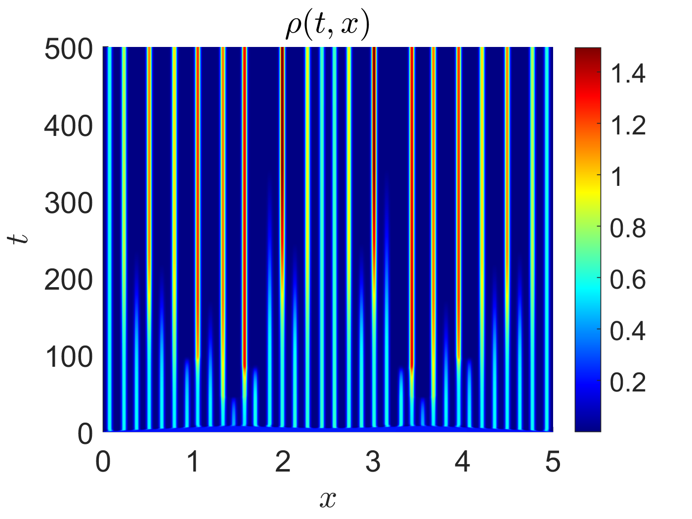

Finally, in Figure 5 we compare the different evolution in case of three different sensing kernels, namely a Dirac delta, a Heavyside function, and a ramp kernel, for the same value of that always fall in the unstable range.
4.3 The case of asymmetric
We now consider Eq. (1) with (5) and (6) allowing the speed probability distribution to depend on , i.e. . In the one-dimensional case it means that cells that go to the right and to the left have different speed distributions.
Following the same procedure as in Section 3, we obtain again Eq.(9) and the local asymptotic equilibria (12), but with with and defined as in (10) and (11) with respectively substituted by and
The local asymptotic equilibria are stationary and homogeneous if and only if
which, on the contrary of the symmetric case, are no longer equal.
Carrying out the same computations as in Section 3, it is convenient to keep Eq.(23) in the following modified form
| (45) |
being defined as in (18).
In order to understand the stability behaviour we will consider . This allows to integrate (45) to get
or
The dispersion relation then reads
| (46) |
where we notice that the speed difference affects the imaginary part while the real part is affected by the mean speed . Furthermore, the fact that implies that the wave frequencies are always complex, hence we expect moving patterns.
According to the type of kernels one then has
| (47) |
where
| (48) |
that reflect the conditions (32), (39), and (42) found in the symmetric case.


In Figure 6 we present some tests in the asymmetric case both with perfectly reflective boundary conditions and periodic boundary conditions in the case of a Dirac delta sensing function. In (a)-(c) we consider adhesion, i.e. in an unstable situation. In particular, Figure 6(c) shows that the imaginary part of the eigenvalue is always stricly positive and in fact both in (a) and (b) there is a moving pattern. In (d)-(f) we have unstable configurations in the case of volume filling Figure 6(f) shows again that as there are complex eigenvalues and therefore we have a moving pattern in the direction that is what we expect as . In Figure 6(g) we present the test with the same value of as in Figure 6(d)-(e) but with . As in Figure 6(g), the pattern is symmetric and there are real eigenvalues (see Figure (i)). In Figure 6(g) the boundary conditions are periodic, but, as , we would obtain the same result with specular reflection boundary conditions. In Figure 6(h) we instead consider adhesion and we have a stable configuration as , even if we have an anisotropic setting as : the transient shows an asymmetric behavior, but the solution goes to a stationary homogeneous case.
5 Discussion
We analyzed the stability properties of a non-local kinetic equation implementing a velocity jump process in which the transition probability models a directional response to a non-local evaluation of the macroscopic cell density. We identified a stability condition (28) that depends on two non-dimensional parametres: that takes into account of the directional response through a non-local measure of the cell density weighted by a sensing kernel , and , that takes into account of the motility properties of cells, specifically their mean speed, sensing radius and tumbling frequency. We proved that if is negative, corresponding to a response that tends to avoid crowding, then instability can occur only for sensing functions that are not non increasing and for small enough. On the other hand, if is positive, corresponding to an adhesion-like behavior, then the homogeneous solution is unstable to long wave for values of that are sufficiently small. Considering that , this means that for fixed instability occurs in stiff regimes, e.g. a large tumbling frequency leads to instability.
On the other hand, if is fixed, the stiffness of the response determines the transition from stability to instability. In the case of increasing at , cells tend to go towards zones that are more crowded. If ) is sufficiently high, there is linear instability, for all the analyzed sensing functions. If is negative, cells tend to go towards regions that are less crowded. In this case instability can be triggered for example in the case in which the sensing function is a Dirac delta, when cells do not evaluate the density in between their position and the sensing position .
Numerical simulations show that the linear stability analysis predicts pattern formation (or stability) quite sharply and it is able to catch the characteristic wavelengths of the pattern.
We restricted to the case in which cell density only affects the direction of motion, e.g., cells turn away if they sense an overcrowded area. Of course, cell density can also affect their speed. This case is currently under study. Actually, the most interesting case is the one in which cell density has an ambivalent effect. For instance, cells are attracted by the other cells because of cell-cell adhesion but at the same time they want to stay away from overcrowding and they do not want to overcome a certain threshold density (volume filling).
Acknowledgements
This work was partially supported by Istituto Nazionale di Alta Matematica, Ministry of Education, Universities and Research, through the MIUR grant Dipartimenti di Eccellenza 2018-2022, Project no. E11G18000350001, and the Scientific Reseach Programmes of Relevant National Interest project n. 2017KL4EF3. NL also acknowledges Compagnia di San Paolo that funds her Ph.D. scholarship.
References
- Armstrong et al., (2006) Armstrong, N. J., Painter, K. J., and Sherratt, J. A. (2006). A continuum approach to modelling cell-cell adhesion. Journal of Theoretical Biology, 243(1):98–113.
- Bitsouni and Eftimie, (2018) Bitsouni, V. and Eftimie, R. (2018). Non-local parabolic and hyperbolic models for cell polarisation in heterogeneous cancer cell populations. Bulletin of Mathematical Biology, 80(10):2600–2632.
- Buttenschön, (2018) Buttenschön, A. (2018). Integro-partial differential equation models for cell-cell adhesion and its application. PhD thesis, University of Alberta.
- Buttenschön and Hillen, (2019) Buttenschön, A. and Hillen, T. (2019). Non-local adhesion models for microorganisms on bounded domains. arXiv:1903.06635.
- Buttenschön and Hillen, (2020) Buttenschön, A. and Hillen, T. (2020). Non-local cell adhesion models: Steady states and bifurcations. arXiv:2001.00286.
- Buttenschön et al., (2018) Buttenschön, A., Hillen, T., Gerisch, A., and Painter, K. J. (2018). A space-jump derivation for non-local models of cell-cell adhesion and non-local chemotaxis. Journal of Mathematical Biology, 76(1):429–456.
- Carrillo et al., (2015) Carrillo, J., Hoffmann, F., and Eftimie, R. (2015). Non-local kinetic and macroscopic models for self-organised animal aggregations. Kinetic Related Models, 8:413–441.
- Colombi et al., (2017) Colombi, A., Scianna, M., and Preziosi, L. (2017). Coherent modelling switch between pointwise and distributed representations of cell aggregates. Journal of Mathematical Biology, 74(4):783–808.
- Colombi et al., (2015) Colombi, A., Scianna, M., and Tosin, A. (2015). Differentiated cell behavior: a multiscale approach using measure theory. Journal of Mathematical Biology, 71:1049–1079.
- Eftimie, (2012) Eftimie, R. (2012). Hyperbolic and kinetic models for self-organized biological aggregations and movement: a brief review. Journal of Mathematical Biology, 65(1):35–75.
- (11) Eftimie, R., de Vries, G., A Lewis, M., and Lutscher, F. (2007a). Modeling group formation and activity patterns in self-organizing collectives of individuals. Bulletin of Mathematical Biology, 69:1537–65.
- Eftimie et al., (2017) Eftimie, R., Perez, M., and Buono, P.-L. (2017). Pattern formation in a nonlocal mathematical model for the multiple roles of the tgf- pathway in tumour dynamics. Mathematical Biosciences, 289:96 – 115.
- (13) Eftimie, R., Vries, G., and Lewis, M. (2007b). Complex spatial group patterns result from different animal communication mechanisms. Proceedings of the National Academy of Sciences of the United States of America, 104:6974–9.
- Filbet and Vauchelet, (2010) Filbet, F. and Vauchelet, N. (2010). Numerical simulation of a kinetic model for chemotaxis. Kinetic and Related Models, 3:B348–B366.
- Hillen et al., (2007) Hillen, T., Painter, K. J., and Schmeiser, C. (2007). Global existence for chemotaxis with finite sampling radius. Discrete Continuous Dynamical Systems - B, 7(1):125–144.
- Lemou and Mieussens, (2008) Lemou, M. and Mieussens, L. (2008). A new asymptotic preserving scheme based on micro-macro formulation for linear kinetic equations in the diffusion limit. SIAM Journal on Scientific Computing, 31(1):334–368.
- (17) Loy, N. and Preziosi, L. (2019a). Kinetic models with non-local sensing determining cell polarization and speed according to independent cues. Journal of Mathematical Biology-accepted (arXiv:1906.11039v3).
- (18) Loy, N. and Preziosi, L. (2019b). Modelling physical limits of migration by a kinetic model with non-local sensing. Preprint (arXiv:1908.08325v1).
- Othmer and Hillen, (2002) Othmer, H. and Hillen, T. (2002). The diffusion limit of transport equations ii: Chemotaxis equations. SIAM Journal of Applied Mathematics, 62:1222–1250.
- Othmer et al., (1988) Othmer, H. G., Dunbar, S. R., and Alt, W. (1988). Models of dispersal in biological systems. Journal of Mathematical Biology, 26(3):263–298.
- Painter and Hillen, (2002) Painter, J. K. and Hillen, T. (2002). Volume-filling and quorum-sensing in models for chemosensitive movement. Canadian Applied Mathematics Quarterly, 10:501–543.
- Painter et al., (2010) Painter, K. J., Armstrong, N. J., and Sherratt, J. A. (2010). The impact of adhesion on cellular invasion processes in cancer and development. Journal of Theoretical Biology, 264(3):1057–1067.
- Painter et al., (2015) Painter, K. J., Bloomfield, M. J., Sherratt, J. A., and Gerisch, A. (2015). A nonlocal model for contact attraction and repulsion in heterogeneous cell populations. Bulletin of Mathematical Biology, 77:1132–1165.
- Perthame and Yasuda, (2018) Perthame, B. and Yasuda, S. (2018). Stiff-response-induced instability for chemotactic bacteria and flux-limited keller–segel equation. Nonlinearity, 31(9):4065–4089.
- Plaza, (2019) Plaza, R. G. (2019). Derivation of a bacterial nutrient-taxis system with doubly degenerate cross-diffusion as the parabolic limit of a velocity-jump process. Journal of Mathematical Biology, 78:1681–1711.
- Schmeiser and Nouri, (2017) Schmeiser, C. and Nouri, A. (2017). Aggregated steady states of a kinetic model for chemotaxis. Kinetic and Related Models, 10(1):313 – 327.
- Stroock, (1974) Stroock, D. W. (1974). Some stochastic processes which arise from a model of the motion of a bacterium. Zeitschrift für Wahrscheinlichkeitstheorie und Verwandte Gebiete, 28(4):305–315.
- Tosin and Frasca, (2011) Tosin, A. and Frasca, P. (2011). Existence and approximation of probability measure solutions to models of collective behaviors. Networks Heterogeneous Media, 6(1):561–596.