Bifurcation and stability of downflowing gyrotactic micro-organism suspensions
in a vertical pipe

We consider a downward fluid flow in a cylindrical vertical pipe, in which a puller type of spherical gyrotactic micro-organisms are suspended (e.g. Chlamydomonas nivalis, Dunaliella and Volvox). We express the position of a point in space in terms of cylindrical co-ordinates $r^{*}$, $\psi^{*}$ and $z^{*}$, the radial, azimuthal and streamwise (or axial) co-ordinates, and the corresponding unit vectors $\mathbf{i}$, $\mathbf{j}$ and $\mathbf{k}$. The fluid has density $\rho^{*}$ and kinematic viscosity $\nu^{*}$, and the gravity is in the same direction as $z^{*}$. The local coordinates of $\mathbf{e}=(e_{1},e_{2},e_{3})$ are introduced for the swimming orientation of the cells, and are defined on the surface of unit sphere (i.e. $\|\mathbf{e}\|=1$), where $e_{1}$, $e_{2}$ and $e_{3}$ indicate the radial, upward ($-z^{*}$) and azimuthal components, respectively. Both of the coordinate systems and the flow geometry are sketched in figure 1. We will also repeat some of the key assumptions made in Hwang & Pedley 2014a; Hwang & Pedley 2014b, where a more detailed discussion and justifications on the assumptions in the present study can be found. The fluid motion is described by the following equations:

Here, the velocity, $\mathbf{u}^{*}=(v^{*},w^{*},u^{*})$, is resolved into the cylindrical components, $p^{*}$ is the pressure, $n^{*}$ the cell number density, $\upsilon^{*}$ the volume of a single cell and $g^{\prime*}=g^{*}\Delta\rho^{*}/\rho^{*}$ the reduced gravity, where $g^{*}$ and $\Delta\rho^{*}$ are the gravitational acceleration and the density difference between the microorganism and the fluid, respectively. Following Hwang & Pedley 2014b, we neglect the stresslet term $\bnabla^{*}\cdot\boldsymbol{\Sigma}_{p}^{*}$, which would be dominantly contributed by the locomotion of the suspended cells (Pedley & Kessler 1990). For the ‘puller’-type swimmers, the stresslet term $\boldsymbol{\Sigma}_{p}^{*}$ is not, in general, responsible for the generation of any instabilities (Saintillan & Shelley 2007; Saintillan & Shelley 2008; Pedley 2010a). This term is also negligible compared to the negative buoyancy (Pedley & Kessler 1990). We will also neglect any near-field cell-cell interactions (Kessler et al. 1992; Ishikawa & Pedley 2007) based on the assumption that the suspension is dilute enough. The validity of the assumption of dilute suspension here will be revisited later in §5.2.

Now, we introduce the transport equation for the cell concentration given in the form of an advection-diffusion equation:

where $\mathbf{u}^{*}+V^{*}_{c}\langle\mathbf{e}\rangle$ is the advection velocity, in which $V^{*}_{c}$ is the cell swimming velocity assumed to be constant and $\langle\mathbf{e}\rangle$ represents the locally ensemble-averaged swimming orientation vector, and ${\mathsfbi{D}}_{m}^{*}$ is the ‘effective’ diffusivity tensor, the detailed definition of which will be introduced below with the subscript $m$. Here, we note that the diffusivity tensor ${\mathsfbi{D}}_{m}^{*}$ is designed to model the spatio-temporal dispersion of the cells phenomenologically. It models the random walk originating from the cell motility and the random cell orientation. Whilst it can also incorporate translational Brownian motion, because the typical size of the cells of interest in the present study (e.g. Chlamydomonas) is too large to experience such a thermal fluctuation, we neglect this here (Pedley & Kessler 1992; Saintillan 2018, see).

Based on (3), we now introduce two models for $\langle\mathbf{e}\rangle$ and ${\mathsfbi{D}}_{m}^{*}$. The first model, often called the Fokker-Planck model, was first introduced by Pedley & Kessler 1990. The second model is based on the GTD theory, first proposed by Brenner 1980. This theory was previously applied to gyrotactic micro-organisms by Hill & Bees 2002 and Manela & Frankel 2003. For simplicity, hereafter, we shall refer to the Fokker-Planck model as model F, and the model based on GTD theory as model G, respectively. The behaviours of $\langle\mathbf{e}\rangle$ and ${\mathsfbi{D}}_{m}^{*}$ with respect to external velocity gradient in the two models have been extensively discussed in several previous studies (Manela & Frankel 2003; Bearon et al. 2012; Croze et al. 2013; Croze et al. 2017). Therefore, in the following sections, we will introduce them only briefly.

The equations of motion (1), (2), (3), and (4a) are non-dimensionalised by

where $N^{*}$ is the cell concentration if the suspension is set to be uniform, and $h^{*}$ is the pipe radius. The resulting dimensionless equations are

The basic state of (10) is first calculated by assuming that the velocity and cell-concentration fields are steady, axisymmetric and homogeneous along the axial direction: i.e.

The basic-state pressure $P_{0}(r,z)$ is obtained by integrating (10b) in the radial direction:

and the hydrostatic pressure gradient balancing out the gravitational term (i.e. $Ri$) in (12a).

Removal of the hydrostatic balance from (10) then yields the following equations for basic state:

Here, the subscript $0$ in $\langle e_{r}\rangle_{0}$ and ${D}_{rr,0}$ indicates the variables from §2.3, which are used for the calculation of steady basic state.

Since the total number of the cells is preserved over the given control volume, we impose the normalisation condition for the cell concentration,

The flow rate $Q$ is assumed to be given, such that

Now, we consider a small perturbation about the basic state:

where $\mathbf{u_{0}}=(0,0,U(r))$, $\mathbf{u^{\prime}}=(v^{\prime},w^{\prime},u^{\prime})$ and $\epsilon\ll 1$. We also define $\boldsymbol{\Omega_{0}}=\nabla\wedge\mathbf{u_{0}}$, $\boldsymbol{\Omega}^{\prime}=\nabla\wedge\mathbf{u}^{\prime}$, $\mathsfbi{G_{0}}=\nabla\mathbf{u_{0}}/D_{R}$ and $\mathsfbi{G}^{\prime}=\nabla\mathbf{u}^{\prime}/D_{R}$ accordingly. Here, we note that the axial velocity perturbation and the cell concentration over a given control volume $V_{0}$ should satisfy

as the flow rate $Q$ is fixed and the total number of the cells over the entire domain is preserved in time. The linearised equations for the small perturbation are then given as

Here, $\mathsfbi{D}^{\prime}_{m}$ and $\langle\mathbf{e}\rangle^{\prime}$ are computed by linearising (10d) and (10j) in a similar manner to Hwang & Pedley 2014a; Hwang & Pedley 2014b. The detailed set of lengthy linearised equations can be found in Appendix A.

Finally, the following normal-mode solution is introduced for linear stability analysis:

where $\alpha$ is the real axial wavenumber, $m$ the wavenumber in the azithumal direction (positive integer), and $\omega$ the complex frequency. Substitution of the normal-mode solution into (18) yields an eigenvalue problem, as detailed in Appendix B.

To obtain the basic state from (13) and subsequently examine its stability, $\langle\mathbf{e}\rangle$ and $\mathsfbi{D}_{m}$ in (10c) need to be computed as a function of $\boldsymbol{\Omega}/D_{R}$ (model F and G) and $\mathsfbi{G}$ (model G): see §2.2. The steady solution $f(\mathbf{e})$ to (10d) is obtained using the solver identical to that of Hwang & Pedley 2014a, and the reader may refer to §3 in Hwang & Pedley 2014a for the detailed result on $\langle\mathbf{e}\rangle$ and $\mathsfbi{D}_{F}$. As for model G, the mean swimming orientation vector $\langle\mathbf{e}\rangle$ is the same as the one for model F. Therefore, only $\mathsfbi{D}_{G}$ used for model G needs to be obtained. With the same discretisation schemes and resolution used for (10d) in Hwang & Pedley 2014a, (10j-10k) are solved to obtain $\mathsfbi{D}_{G}$. The numerical results agree very well with the ones given by Bearon et al. 2012. Similarly, $\langle\mathbf{e}\rangle^{\prime}$ and $\mathsfbi{D}_{m}^{\prime}$ used in (18e) are calculated by applying the same discretisation schemes to the equations in Appendix A.

In order to compute the basic state, the radial direction of (13) is discretised using a Chebyshev collocation method described in Weideman & Reddy 2000. Two solvers have been written in MATLAB: one is based on a Newton-Ralphson method, and the other solves the unsteady version of (13) to obtain its steady solution, the latter of which is used to study the stability of the basic state to axially uniform and radially independent perturbation. The solutions from the two solvers have been validated against each other when stable solutions are admitted. They are found to be identical up to the given numerical precision. Finally, for the purpose of studying bifurcation of the basic state, the Newton-Raphson solver is combined with a pseudo-arclength continuation algorithm (see §3).

For the linear stability, the radial direction of (35) is discretised using the same discretisation method as the one for the basic state. The discretised eigenvalue problem is solved using the function eig in MATLAB. The computation is performed with $N_{r}=175$, showing no difference from the results with $N_{r}=100$. The computed eigenvalues for $\mathrm{Ri}=0$ are validated against pipe flow stability data of Schmid & Henningson 1994; Schmid & Henningson 2001 and Meseguer & Trefethen 2003 with excellent agreement.

A list of parameters and their values used in the present study are summarised in table 1. Here, it should be noted that $\tau^{*}$ is not a free parameter, as mentioned in §2.2. Instead, $\tau^{*}$ is set, such that model F and G provide consistent and quantitatively comparable results. Therefore, in the present study, we follow the approach of Bearon et al. 2012, in which $\tau^{*}$ is chosen to match $D_{G,rr}$ with $D_{F,rr}$ in the absence of any flow (i.e. stationary medium). This gives $\tau=0.36$, consistent with that of Bearon et al. 2012.

In this study, the radius of the cylindrical pipe is chosen to be around $0.2$cm, so that we obtain results comparable with the same as Hwang & Pedley 2014b, at around $0.2$cm. The parameters for cell’s biological properties, including cell swimming speed $V_{c}^{*}$, gyrotactic time scale $\beta^{*}$, relative cell density $\Delta\rho/\rho$ and rotational diffusivity $D_{R}^{*}$, are taken for C. nivalis from previous studies (Pedley & Kessler 1990; Bees & Hill 1998; Pedley 2010b; Hwang & Pedley 2014b, e.g.), except the shape of the cell which we assume to be spherical. As in the linear stability analysis of Hwang & Pedley 2014b and the experiment of Croze et al. 2017, only the flow rate $Q$ and the background cell concentration (represented by $Ri$) are varied in this study. Based on the parameter values given in table 1, the dimensionless parameters and their values examined are given in table 2.

At very low flow rate (i.e. $Q\rightarrow 0$), model F and G share the same asymptotic value for $\langle\mathbf{e}\rangle$ and the radial diagonal component of $\mathsfbi{D}_{m}$ (see Bearon et al. 2012 and figure 7). Therefore, the two models would give almost identical result when $Q$ is small enough. Hence, here we report the result from model G first in this case.

When $Q=0$, a stationary uniform suspension (i.e. $U(r)=0$ and $N(r)=1$) is a solution to (13). However, a further numerical search has also found that there exists another solution at $Q=0$ featured with non-trivial $U(r)$ and $N(r)$, consistent with Bees & Croze 2010. Bifurcation diagrams of these two solutions with respect to $Ri$ are shown for small positive $Q$ in figure 2, where the centreline concentration $N(0)$ and axial velocity $U(0)$ are used to represent the state of the steady solutions. For $Q=0$, the two solutions meet at $Ri=Ri_{c}(\simeq 189.9)$, and their stability has been checked using the unsteady solver described in §2.6. The stationary solution ($U(r)=0$ and $N(r)=1$) is found to be stable for $Ri<Ri_{c}$, but becomes unstable for $Ri>Ri_{c}$. On the other hand, the non-trivial solution, featured with a downflow and a high cell concentration along the pipe axis, is unstable for $Ri<Ri_{c}$. This solution gains its stability when $Ri>Ri_{c}$, and the form of the solution is subsequently changed with an upflow and a lower cell concentration along the pipe axis. The interchange of the stability of the two solutions at $Ri=Ri_{c}$ indicates that the stationary suspension in the vertical pipe experiences a transcritical bifurcation with $Ri$.

When a small downflow ($Q>0$) is applied, the transcritical bifurcation point given at zero flow rate turns into a saddle-node point. At $Ri>Ri_{c}$, the axial velocity is upward instead of downward (i.e. $U(0)<0$), even though the overall net flow is downward ($Q>0$). If a small upflow ($Q<0$) is applied instead, then the opposite is true, as shown by the grey area in figure 2. The transition from a transcritical to a saddle-node bifurcation is a consequence of an imperfect bifurcation caused by the addition of a small non-zero flow rate. This behaviour of the solutions with two parameters, $Ri$ and $Q$, can be understood within the framework of co-dimension two bifurcation (i.e. bifurcation with two parameters). The overall bifurcation is also closely related to how the system would evolve with the flow direction. However, given the scope of the present study, we shall only focus on the downflowing case and leave the upflowing case as future work.

The solution featured with $N(0)>1$ and $U(0)>0$ in figure 2 is further continued for much higher flow rates with model F. Figure 3( a ) shows the result from such continuation with model F, in which the concentration at the pipe axis $N(0)$ is used to represent the state of the corresponding steady solution. At sufficiently low flow rate ($Q\lesssim 1$), the bifurcation of the solutions featured with two saddle-node points (highlighted by the crosses in figure 3( a )), indicating the emergence of three solutions at the given flow rate. With the increasing order of $N(0)$, the three types of solutions will be denoted by lower, middle and upper branches, respectively, and they are visualised in figure 4. Here, we note that $N(0)$ was found to uniquely represent each solution per parameter set, and hence was used as a representation for each solution. In general, as the solution is continued from the lower to upper branch, both the velocity and cell-concentration profiles near the pipe axis ($r=0$) tend to be sharper. This is expected because the lower-branch state is a homotopy of the uniform suspension obtained with increasing flow rate (i.e. state without gyrotactic instability), while the middle- and upper-branch states are homotopy of nonlinearly developed plumes from the gyrotatic instability at zero flow rate (i.e. state with nonlinearly staruated gyrotactic instability). Examination of the stability of each solution to axially and radially uniform perturbations (i.e. unsteady calculation of the basic state) reveals that the lower and upper branches are stable, whereas the middle one is unstable, indicating bistable nature of the basic state featured with hysteresis.

As the flow rate $Q$ is further increased, the two saddle-node points become closer. They eventually merge and disappear with the increasing $Q$. The curves in figure 3( b ) shows how the two saddle-node points evolved with $Q$ in the $Q-Ri-N(0)$ space. At the bottom of this figure, the trajectories of the two saddle-node points are projected onto the $Q-Ri$ plane to visualise how the $Ri$ values at these points change with $Q$. The two saddle-node points in the $Q-Ri$ plane indeed merge as $Q$ increases. Beyond this merging point, the bistable behaviour of the steady solutions disappears, as there exits only single steady solution. This type of codimension two bifurcation is a cusp bifurcation (Zeeman 1976; Thom 1989, see). Further discussion on the bifurcation in relation to previous experimental observations will be given in §5.3.

Lastly, it is worth mentioning that, in model F, the density at the pipe axis $N(0)$ decreases with increasing $Ri$ for sufficiently large $Ri$ (see the upper branch in figure 3( a )). As discussed in Hwang & Pedley 2014b, the decrease of $N(0)$ is the direct consequence of increasing $D_{rr}$ with the increase of background base-flow shear (see figure 7( b ) of this paper and figure 3$(b)$ of Hwang & Pedley 2014b), which smooths out the gyrotactic focusing near the pipe axis.

Now, we compare the steady basic-state solutions obtained from model F to those from model G. Figure 5( a ) shows the bifurcation diagram of the steady solution obtained using model G. When the cell concentration at the pipe axis is relatively small (i.e. $N(0)<10^{2}$), the same kind of cusp bifurcation is seen in this case (compare with figure 3( a )). Also, the related form of the steady solutions is qualitatively identical to that obtained with model F, as shown in figure 6. However, as the solution is continued further from the middle branches, its behaviour turns out to be very different from that obtained with model F. In particular, for all the flow rates considered, the bifurcation curves do not properly form the upper branches, contrary to the model F (compare with figure 3( b )). Indeed, irrespective of the flow rate $Q$, the continued solution from the middle branch asymptotically exhibits a singular behaviour at $Ri=Ri_{s}(\simeq 59.86)$ in figure 5( a )), implying $N(0)\rightarrow\infty$ with the continuation. This suggests that a steady downflowing upper-branch solutions may not necessarily exist for $Ri>Ri_{s}$.

The origin of the singularity in the steady solution can be further studied from the following explicit form of $N(r)$ obtained with (13c) and (13d) Bees & Croze 2010:

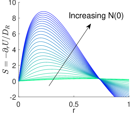
This form of the solution indicates that the singularity would be directly related to the behaviour of $\langle e_{r}\rangle_{0}/D_{rr,0}$ with prescribed background shear $S(\equiv-1/D_{R}dU/dr)$. Note that $S$ is varying with the radial position $r$ (figure 8) because of the coupling via the negative buoyancy. In effect, $S(r)$ can also be interpreted as the local rotary Péclet number. Figure 7( a ) shows the behaviour of $\langle e_{r}\rangle_{0}/D_{rr,0}$ with the background shear $S$ for both model F and G (see also figure 1$(f)$ in Bearon et al. 2012). For model F, the values of $\langle e_{r}\rangle_{0}/D_{rr,0}$ are bounded between a relatively small negative value ($\min(\langle e_{r}\rangle_{0}/D_{rr,0})=-3.47$) and zero for all the values of $S$. However, in the case of model G, $\langle e_{r}\rangle_{0}/D_{rr,0}$ monotonically decreases with $S$ and is roughly linearly proportional to $S$ for sufficiently large $S$ (figure 7( a )). It should be mentioned that this difference in $\langle e_{r}\rangle_{0}/D_{rr,0}$ between model F and G must originate from the difference in the translational diffusivity, because they share exactly the same $\langle e_{r}\rangle$ (see also §2). This is shown in figure 7( b ).

Figure 8 visualises the radial profiles of $S(r)$ and $\langle e_{r}\rangle_{0}/D_{rr,0}(r)$ for model F and G along the continuation curves at $Q=2.1$. As the solution is continued from the lower to the upper branch, the absolute values of $S(r)$ monotonically increase for both model F and G (figures 8$a$, $b$) However, $\langle e_{r}\rangle_{0}/D_{rr,0}(r)$ do not behave like $S(r)$. In particular, $\langle e_{r}\rangle_{0}/D_{rr,0}(r)$ for model F is bounded due to the nature shown in figure 7( a ). As a result, $\langle e_{r}\rangle_{0}/D_{rr,0}(r)$ in figure 8( b ) is bounded, whereas that in 8( d ) is not. This suggests that the singularity developed at $Ri_{s}$ from model G originates from the unboundedness of $\langle e_{r}\rangle_{0}/D_{rr,0}(S)$.

If the behaviour of $\langle e_{r}\rangle_{0}/D_{rr,0}$ in model G is further simplified, the $Ri_{s}$ in figure 5( b ) can be predicted analytically. For this purpose, we consider a simplified model for $\langle e_{r}\rangle_{0}/D_{rr,0}$, in which the translational diffusivity is set such that $\langle e_{r}\rangle_{0}/D_{rr,0}$ is linearly proportional to the background shear $dU/dr$:

In this model, $\langle e_{r}\rangle_{0}$ is kept to be the same as that used in both model F and G, and $\eta$ is obtained from the slope of $\langle e_{r}\rangle_{0}/D_{rr,0}$ for $S=0$: i.e. $\eta\equiv-\partial(\langle e_{r}\rangle_{0}/D_{rr,0})/\partial S|_{S=0}$. The behaviour of this simplified model is shown in figure 7( a ), in which $\langle e_{r}\rangle_{0}/D_{rr,0}$ of this model behaves similarly to that of model G with $\eta=1.10$. We shall refer to this model as the ‘linearised model’.

Coincidentally, the behaviour of $\langle e_{r}\rangle_{0}/D_{rr,0}$ against $S$ in this ‘linearised model’ is the same as that of Kessler 1986a. In Kessler 1986a, $\langle e_{r}\rangle_{0}$ is linear to shear rate $S$ and $D_{rr,0}$ is constant. In contrast, in both model G and the subsequent ‘linearised model’, $D_{rr,0}\sim S^{-2}$ and $\langle e_{r}\rangle_{0}\sim S^{-1}$ as $S$ increases towards infinity. As a result, the ‘linearised model’ shares the same linear behaviour in $\langle e_{r}\rangle_{0}/D_{rr,0}(S)$ with the simpler model of Kessler 1986a, even though their approximations for $\langle e_{r}\rangle_{0}$ and $D_{rr,0}$ respectively are different. In the following, we will exploit the similiarity in $\langle e_{r}\rangle_{0}/D_{rr,0}(S)$ between the ‘linearised model’ and Kessler 1986a to understand the bifurcation.

Bifurcation of the steady solutions of the linearised model is shown in figure 9 for $\eta=1.10$. The bifurcation diagram of the linearised model confirms the behaviour qualitatively similar to that of model G: as the solution is continued from the lower to upper branch, the cell concentration at the pipe axis gradually becomes singular at $Ri\simeq Ri_{s}(=57.68)$ irrespective of $Q$ (compare with figure 5( a )). The only qualitative difference between figure 5( a ) and figure 9 is the small extra bumpy behaviour in the bifurcation curves of model G, likely the consequence of the nonlinear behaviour of $\langle e_{r}\rangle_{0}/D_{rr,0}$ in this model. This suggests that the singularity at the centreline cell concentration in model G indeed originates from the monotonically decreasing $\langle e_{r}\rangle_{0}/D_{rr,0}$ with the background shear rate $S$. In fact, as $S\rightarrow\infty$, $\langle e_{r}\rangle_{0}$ scales with $S^{-1}$ while $D_{rr,0}$ scales with $S^{-2}$, hence $\langle e_{r}\rangle_{0}/D_{rr,0}$ scales with $S$ (Bearon et al. 2012). This implies that the origin of the singularity in $N(0)$ is essentially associated with the lack of translational diffusion flux relative to the advection flux caused by swimming in the radial direction in model G, as the local shear rate $S$ increases with $N(0)$ towards infinity along the continuation.

The emergence of this singularity can be more precisely analysed. We now consider the following equation for $N(r)$, which can be obtained from (13) with $D_{rr,0}$ in (21) of the linearised model:

where $\gamma={\eta RiRe}/8$ and $G=\eta\partial U/\partial r|_{r=1}$. Since $N(r)$ near the singular regime is highly concentrated near the pipe axis, we assume that the cell concentration is highly focused in a small region around the axis: i.e. $r\in[0,\epsilon]$. Then, from the constraint of $N(r)$ given by (14), $N(r)\sim O(\epsilon^{-2})$ in $r\in[0,\epsilon]$. Therefore, in this region, we can introduce a relevant rescaling of the radial coordinate $r=\epsilon R$, where $R$ is of order unity, and define a normalised profile $N_{0}(R)=N(r/\epsilon)/N(0)$. Then, at $O(\epsilon^{-2})$, (22) is approximated as

Now, it is evident that (23) does not contain $G$ anymore, although it still describes the behaviour of most of the cell concentration in the suspension. This implies that, in the regime where the singular solution nearly develops, the form of the steady basics-state solution should approximately be independent of pressure gradient as well as of flow rate for $r\in[0,\epsilon]$, confirming the numerical result for $N(0)>O(10^{3})$ shown in figure 9.

References

- Bearon et al. (2012) Bearon, Rachel N., Bees, M. A. & Croze, O. A. 2012 Biased swimming cells do not disperse in pipes as tracers: A population model based on microscale behaviour. Phys. Fluids 24 (12), 121902.
- Bearon & Hazel (2015) Bearon, R. N. & Hazel, A. L. 2015 The trapping in high-shear regions of slender bacteria undergoing chemotaxis in a channel. J. Fluid Mech. 771, R3.
- Bearon et al. (2011) Bearon, Rachel N., Hazel, A. L. & Thorn, G. J. 2011 The spatial distribution of gyrotactic swimming micro-organisms in laminar flow fields. J. Fluid Mech. 680, 602–635.
- Bees (2020) Bees, Martin A. 2020 Advances in Bioconvection. Annu. Rev. Fluid Mech. 52 (1), 449–476.
- Bees & Croze (2010) Bees, M. A. & Croze, O. A. 2010 Dispersion of biased swimming micro-organisms in a fluid flowing through a tube. Proc. R. Soc. A Math. Phys. Eng. Sci. 466, 2057–2077.
- Bees & Hill (1997) Bees, M. A. & Hill, N. A. 1997 Wavelengths of bioconvection patterns. J. Exp. Biol. 200 (Pt 10), 1515–1526.
- Bees & Hill (1998) Bees, M. A. & Hill, N. A. 1998 Linear bioconvection in a suspension of randomly swimming, gyrotactic micro-organisms. Phys. Fluids 10 (8), 1864–1881.
- Berke et al. (2008) Berke, Allison P., Turner, Linda, Berg, Howard C. & Lauga, Eric 2008 Hydrodynamic attraction of swimming microorganisms by surfaces. Phys. Rev. Lett. 101 (3), 1–4.
- Brenner (1980) Brenner, Howard 1980 General Theory of Taylor Dispersion Phenomena. PCH. Physicochem. Hydrodyn. 1 (2-3), 91–123.
- Croze et al. (2017) Croze, O. A., Bearon, Rachel N. & Bees, M. A. 2017 Gyrotactic swimmer dispersion in pipe flow: Testing the theory. J. Fluid Mech. 816, 481–506.
- Croze et al. (2013) Croze, O. A., Sardina, G., Ahmed, M., Bees, M. A. & Brandt, L. 2013 Dispersion of swimming algae in laminar and turbulent channel flows: consequences for photobioreactors. J. R. Soc. Interface 10 (81).
- Denissenko & Lukaschuk (2007) Denissenko, P. & Lukaschuk, S. 2007 Velocity profiles and discontinuities propagation in a pipe flow of suspension of motile microorganisms. Phys. Lett. Sect. A Gen. At. Solid State Phys. 362 (4), 298–304.
- Elgeti & Gompper (2013) Elgeti, Jens & Gompper, Gerhard 2013 Wall accumulation of self-propelled spheres. EPL (Europhysics Lett.) 101 (4), 48003.
- Ezhilan & Saintillan (2015) Ezhilan, Barath & Saintillan, David 2015 Transport of a dilute active suspension in pressure-driven channel flow. J. Fluid Mech. 777, 482–522.
- Frankel & Brenner (1991) Frankel, I. & Brenner, Howard 1991 Generalized Taylor dispersion phenomena in unbounded homogeneous shear flows. J. Fluid Mech. 230, 147–181.
- Frankel & Brenner (1993) Frankel, I. & Brenner, Howard 1993 Taylor dispersion of orientable brownian particles in unbounded homogeneous shear flows. J. Fluid Mech. 255, 129–156.
- Hernandez-Ortiz et al. (2005) Hernandez-Ortiz, Juan P., Stoltz, Christopher G. & Graham, Michael D. 2005 Transport and collective dynamics in suspensions of confined swimming particles. Phys. Rev. Lett. 95 (20), 1–4.
- Hill & Bees (2002) Hill, N. A. & Bees, M. A. 2002 Taylor dispersion of gyrotactic swimming micro-organisms in a linear flow. Phys. Fluids 14 (8), 2598–2605.
- Hill & Häder (1997) Hill, N. A. & Häder, D. P. 1997 A biased random walk model for the trajectories of swimming micro-organisms. J. Theor. Biol. 186 (4), 503–526.
- Hill et al. (1989) Hill, N. A., Pedley, T. J. & Kessler, John O. 1989 Growth of bioconvection patterns in a suspension of gyrotactic micro-organisms in a layer of finite depth. J. Fluid Mech. 208, 509–543.
- Hinch & Leal (1972a) Hinch, E. J. & Leal, L. G. 1972a Note on the rheology of a dilute suspension of dipolar spheres with weak Brownian couples. J. Fluid Mech. 56 (4), 803–813.
- Hinch & Leal (1972b) Hinch, E. J. & Leal, L. G. 1972b The effect of Brownian motion on the rheological properties of a suspensions of non-spherical particles. J. Fluid Mech. 52 (4), 683–712.
- Hwang & Pedley (2014a) Hwang, Yongyun & Pedley, T. J. 2014a Bioconvection under uniform shear: linear stability analysis. J. Fluid Mech. 738, 522–562.
- Hwang & Pedley (2014b) Hwang, Yongyun & Pedley, T. J. 2014b Stability of downflowing gyrotactic microorganism suspensions in a two-dimensional vertical channel. J. Fluid Mech. 749, 750–777.
- Ishikawa & Pedley (2007) Ishikawa, Takuji & Pedley, T. J. 2007 Diffusion of swimming model micro-organisms in a semi-dilute suspension. J. Fluid Mech. 588, 437–462.
- Jeffery (1922) Jeffery, G. B. 1922 The motion of ellipsoidal particles immersed in a viscous fluid. Proc. R. Soc. London. Ser. A 102, 161–179.
- Jiang & Chen (2019) Jiang, Weiquan & Chen, Guoqian 2019 Dispersion of active particles in confined unidirectional flows. J. Fluid Mech. 877, 1–34.
- Jiang & Chen (2020) Jiang, Weiquan & Chen, Guoqian 2020 Dispersion of gyrotactic micro-organisms in pipe flows. J. Fluid Mech. 889, A18.
- Kessler (1984) Kessler, John O. 1984 Gyrotactic Buoyant Convection and Spontaneous Pattern Formation in Algal Cell Cultures. In Nonequilibrium Coop. Phenom. Phys. Relat. Fields (ed. Manuel G Velarde), pp. 241–248. Boston, MA: Springer US.
- Kessler (1985a) Kessler, John O. 1985a Co-operative and concentrative phenomena of swimming micro-organisms. Contemp. Phys. 26, 147–166.
- Kessler (1985b) Kessler, John O. 1985b Hydrodynamic focusing of motile algal cells. Nature 313, 218–220.
- Kessler (1986a) Kessler, John O. 1986a Individual and collective fluid dynamics of swimming cells. J. Fluid Mech. 173, 191–205.
- Kessler (1986b) Kessler, John O. 1986b The external dynamics of swimming micro-organisms. Prog. Phycol. Res. 4, 257–307.
- Kessler et al. (1992) Kessler, John O., Hill, Nicholas A. & Hader, Donat-P. 1992 Orientation of swimming flagellates by simultaneously acting external factors. J. Phycol. 28 (6), 816–822.
- Koch & Shaqfeh (1989) Koch, D. L. & Shaqfeh, Eric S. G. 1989 The instability of a dispersion of sedimenting spheroids. J. Fluid Mech. 209, 521–542.
- Manela & Frankel (2003) Manela, A. & Frankel, I. 2003 Generalized Taylor dispersion in suspensions of gyrotactic swimming micro-organisms. J. Fluid Mech. 490, 99–127.
- Maretvadakethope et al. (2019) Maretvadakethope, Smitha, Keaveny, Eric E. & Hwang, Yongyun 2019 The instability of gyrotactically trapped cell layers. J. Fluid Mech. 868, R5.
- Mehandia & Nott (2008) Mehandia, Vishwajeet & Nott, Prabhu R. 2008 The collective dynamics of self-propelled particles. J. Fluid Mech. 595, 239–264.
- Meseguer & Trefethen (2003) Meseguer, A & Trefethen, L. N. 2003 Linearized pipe flow to Reynolds number . J. Comput. Phys. 186 (1), 178–197.
- O’Malley & Bees (2012) O’Malley, Stephen & Bees, Martin A. 2012 The Orientation of Swimming Biflagellates in Shear Flows. Bull. Math. Biol. 74 (1), 232–255.
- Pedley (2010a) Pedley, T. J. 2010a Collective Behaviour of Swimming Micro-organisms. Exp. Mech. 50 (9), 1293–1301.
- Pedley (2010b) Pedley, T. J. 2010b Instability of uniform micro-organism suspensions revisited. J. Fluid Mech. 647, 335–359.
- Pedley et al. (1988) Pedley, T. J., Hill, N. A. & Kessler, John O. 1988 The growth of bioconvection patterns in a uniform suspension of gyrotactic micro-organisms. J. Fluid Mech. 195, 223.
- Pedley & Kessler (1990) Pedley, T. J. & Kessler, John O. 1990 A new continuum model for suspensions of gyrotactic micro-organisms. J. Fluid Mech. 212, 155–182.
- Pedley & Kessler (1992) Pedley, T. J. & Kessler, John O. 1992 Hydrodynamic Phenomena In Suspensions Of Swimming Microorganisms. Annu. Rev. Fluid Mech. 24 (1), 313–358.
- Saintillan (2018) Saintillan, David 2018 Rheology of Active Fluids. Annu. Rev. Fluid Mech. 50 (1), 563–592.
- Saintillan et al. (2006) Saintillan, David, Shaqfeh, Eric S. G. & Darve, Eric 2006 The growth of concentration fluctuations in dilute dispersions of orientable and deformable particles under sedimentation. J. Fluid Mech. 553, 347.
- Saintillan & Shelley (2007) Saintillan, David & Shelley, Michael J. 2007 Orientational order and instabilities in suspensions of self-locomoting rods. Phys. Rev. Lett. 99 (5), 1–4.
- Saintillan & Shelley (2008) Saintillan, David & Shelley, Michael J. 2008 Instabilities and pattern formation in active particle suspensions: Kinetic theory and continuum simulations. Phys. Rev. Lett. 100 (17), 178103.
- Schmid & Henningson (1994) Schmid, Peter J. & Henningson, Dan S. 1994 Optimal energy density growth in Hagen–Poiseuille flow. J. Fluid Mech. 277, 197–225.
- Schmid & Henningson (2001) Schmid, Peter J. & Henningson, Dan S. 2001 Stability and Transition in Shear Flows, Applied Mathematical Sciences, vol. 142. New York, NY: Springer New York.
- Spagnolie & Lauga (2012) Spagnolie, Saverio E. & Lauga, Eric 2012 Hydrodynamics of self-propulsion near a boundary: predictions and accuracy of far-field approximations. J. Fluid Mech. 700, 105–147.
- Thom (1989) Thom, Rene 1989 Structural Stability And Morphogenesis. CRC Press.
- Underhill et al. (2008) Underhill, Patrick T., Hernandez-Ortiz, Juan P. & Graham, Michael D. 2008 Diffusion and spatial correlations in suspensions of swimming particles. Phys. Rev. Lett. 100 (24), 1–4.
- Vennamneni et al. (2020) Vennamneni, Laxminarsimharao, Nambiar, Sankalp & Subramanian, Ganesh 2020 Shear-induced migration of microswimmers in pressure-driven channel flow. J. Fluid Mech. 890.
- Vladimirov et al. (2000) Vladimirov, V. A., Denissenko, P. V., Pedley, T. J., Wu, M. & Moskalev, I. S. 2000 Algal motility measured by a laser-based tracking method. Mar. Freshw. Res. 51 (6), 589.
- Weideman & Reddy (2000) Weideman, J A C & Reddy, S C 2000 A MATLAB Differentiation Matrix Suite. ACM Trans. Math. Softw. 26 (4), 465–519.
- Zeeman (1976) Zeeman, E. C. 1976 Catastrophe Theory. Sci. Am. 234 (4), 65–83.