Transport in two dimensional Rashba electron systems doped with interacting magnetic impurities

Two dimensional electron systems with Rashba spin-orbit coupling (SOC) play leading roles in novel spintronics. Locking of the spin degrees of freedom with the spatial motion of itinerant electrons splits the spin-degenerate band of the system into two parabolic bands with opposite spin-helicity intersecting each other at the band-crossing point (BCP). The presence of two bands with different spin states is one of the hallmarks of two dimensional Rashba electron systems (2DRSs) in spintronics applications, especially in the manipulation of spin state of electrons in the absence of external magnetic fields.Rashba 1960; Vas’ko 1979; Bychkov and Rashba 1984; Sharma 2005; Zutić et al. 2004 Topological changes of Fermi surface and the variations of band structure from two spin states to the valley band with a single spin state in passing through the BCP, lead to several phenomena in low-density regime, Cappelluti et al. 2007; Grimaldi 2005; Wu et al. 2014 such as qualitatively significant modifications of thermoelectric and thermopower properties,Xiao et al. 2016a; Wu et al. 2014 modifications of the classical Dyakonov-Perel mechanism of spin relaxation,Grimaldi 2005 and the enhancement of the superconducting critical temperature in 2DRSs with strong SOC.Cappelluti et al. 2007

Doping of 2DRSs with magnetic impurities leads to many exotic phenomenaNunner et al. 2008; vZitko and Bonvca 2011; Zarea et al. 2012; Isaev et al. 2012; Yan et al. 2012 such as anomalous Hall effect and anisotropic magnetoresistance (AMR). The combined effects of Rashba SOC and localized spins significantly modify the transport properties of the system, they lead to resonantly enhancement of anomalous Hall conductivityNunner et al. 2008 and giant AMR.Výborný et al. 2009 For systems with low impurity concentrations, interactions between magnetic impurities are negligible and the transport properties of the system is properly given by considering single impurity scattering effects,Výborný et al. 2009 however when doping increases these interactions become crucial. One of the effective solution for systems with high impurity concentrations is taking the effects of multiple scatterings into account.Walls et al. 2006 In this paper we use the concept of magnetic clusters and study the effects of magnetic clusters on the transport properties of 2DRSs. Exchange interactions between magnetic impurities cause the formation of clusters where constructed of correlated magnetic impurities fluctuating consistently in the same direction. The clusters’ mean sizes (CMSs) and their number (CN) depend on temperature. The cluster model was first proposed in Refs.[Akabli et al. 2011; Akabli and Diep 2008] for explaining the temperature dependence of the magneto-resistance of magnetic semiconductors, and recently developed for investigating the surface conductivity of three dimensional magnetic topological insulators.Zarezad and Abouie 2018 In this paper by treating magnetic clusters as scattering centers, distributed randomly on the surface of the 2DRSs, and modeling the interaction of itinerant electrons with magnetic clusters by a long-range scattering potential, we demonstrate that the combined effects of Rashba SOC and magnetic clusters cause the system to be anisotropic and the anisotropy strongly depends on both the clusters’ mean size and spin, the strengths of SOC and the locations of Fermi energy with respect to the BCP. We obtain the non-equilibrium distribution functions of electrons in different bands within the semiclassical Boltzmann approach, and compute the conductivity and the AMR of the system in both regimes of above and below the BCP. We demonstrate that for large CMSs the angular dependence of the AMR is unconventional in comparison with conventional ferromagnets. We also show that, there are many contrasts between the transport properties of the system in the two regimes of above and below the BCP.

This paper is organized as follows. In Sec. II, we obtain the band structure of 2DRSs and present the generalized relaxation time approximation in order to find the non-equilibrium distribution functions of electrons in each bands. In Sec. III, we present the explicit form of the conductivities in the two-band regime. In this section we also compare the relaxation times obtained by other approaches. The results of the single band regime are presented in Sec. IV. The summaries and conclusions are given in Sec.V. At the end of this paper we present the details of our calculations in three different appendices.

The Hamiltonian of a 2DRS is given by:

where the first term is the kinetic energy of electrons with effective mass $m$, and the second term is the Rashba SOC with the strength of $\alpha$. The Pauli matrices $\sigma_{x,y}$ indicate spin of electrons, and $k_{x,y}$ are the two components of electrons’ wave vector, ${\bf k}$. The eigenenergies and eigenstates of the Hamiltonian $H_{0}$ are obtained as,

where $n(=\pm)$ represents the Rashba bands, $\varepsilon_{\rm R}=\frac{m\alpha^{2}}{\hbar^{2}}$ is the Rashba energy ($\varepsilon_{\rm R}/2$ is the minimum value of the band $+$ at $k_{\rm R}=\frac{m\alpha}{\hbar^{2}}$), $A$ is the area of the 2DRS, and $\phi=\arctan(k_{y}/k_{x})$ is the polar angle of the ${\bf k}$-vector. In the presence of SOC, the energy spectrum splits into two energy bands + and $-$, intersecting each other at the band-crossing point (BCP), illustrated in Fig. 1.

Strong SOC has been observed in several materials,Ast et al. 2007; Ast et al. 2008; Moreschini et al. 2009; Gierz et al. 2009 such as ${\rm Te}$-terminated surface of the polar semiconductor ${\rm BiTeX}$ (X=I, Br and Cl)Ishizaka and et.al 2011; Eremeev et al. 2012; Eremeev et al. 2013; Landolt et al. 2012; Landolt et al. 2013; Crepaldi et al. 2012 where Rashba SOC is at the order of 1.7-3.8 eV$\mathring{A}$, which is one order of magnitude larger than the Rashba SOC in conventional III-V semiconductor heterostructures.

In a two-dimensional electron system doped with magnetic impurities, the interaction between an electron with spin ${\bm{\sigma}}$ at the position ${\bf r}$, with an impurity with spin ${\bf S}$ located at ${\bf R}$ is given by the following Hamiltonian:

where $J({\bf r}-{\bf R})$ is the exchange coupling. In dilute magnetic systems itinerant electrons interact with individual single magnetic impurities, and the exchange coupling is modeled by Dirac $\delta$ function as $J({\bf r}-{\bf R})\propto J_{0}\delta({\bf r}-{\bf R})$, where $J_{0}$ is a coupling constant at the order of few $meV$.Manchon and Zhang 2008; Liu and Xiong 2006; J.K. Furdyna 1988 When doping of magnetic impurities increases, the interactions between magnetic impurities become significant and we should consider their effects on the transport properties of the system. Actually, the exchange interactions between impurities lead to the formation of various magnetic domains with different sizes in the entire system. These ordered domains which are called ”magnetic clusters”, are constructed of correlated magnetic impurities with the same spin directions. Scattering of electrons by these clusters (rather than single impurities) alters the transport properties of the system.Zarezad and Abouie 2018 In order to investigate the effects of magnetic clusters on the conductivity, we model the scattering potential of electrons by a clusters as:

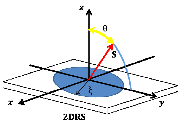
where $\xi$ is clusters’ mean size, depending on both temperature and impurity-impurity exchange coupling, and ${\bm{\sigma}}$ is the spin of magnetic cluster located at ${\bf R}$. The scattering potential in Eq. (5) is long-range and $\xi$ appears as a characteristic length, indicating the range of scattering potential. Without loss of generality, we consider the spins of clusters as classical vectors in $yz$ plane, i.e. ${\bf S}=S(0,\sin\theta,\cos\theta)$, where $\theta$ is the tilt angle of ${\bf S}$ with the axis normal to the surface of the 2DRS (see Fig. 2).

In order to obtain the non-equilibrium distribution function of electrons in the presence of magnetic clusters, we use the semi-classical Boltzmann approach. In the presence of a uniform electric field ${\bf E}$, the non-equilibrium distribution function of electrons in the band $n$, $f_{n}({\bf k},{\bf E})$, satisfies the following relation:

where ${\bf v}_{n}({\bf k})$ is the band velocity, and $f^{0}_{n}$ is the Fermi-Dirac distribution function in the band $n$. By considering elastic scatterings and using detailed balance, the left hand side of Eq. (6) is also written as Schliemann and Loss 2003:

where $w_{n,n^{\prime}}({\bf k},{\bf k}^{\prime})$ is the transition rate between the two eigenstates of the Hamiltonian $H_{0}$ ($\left|{n{\bf k}}\right\rangle$ and $\left|{n^{\prime}{\bf k}^{\prime}}\right\rangle$). Using Eqs. (6) and (7), the Boltzmann equation is written as:

where the interaction between electrons has been neglected.

In the isotropic 2DRSs ($\theta=0$), the scattering rate depends on the angle between ${\bf k}$ and ${\bf k}^{\prime}$ ($\Delta\phi=\phi-\phi^{\prime}$), and relaxation times of electrons in the bands + and $-$ depend only on the magnitudes of ${\bf k}$ and ${\bf k}^{\prime}$. By using standard methods such as modified relaxation time approximation (MRTA)Výborný et al. 2009; Trushin et al. 2009, and other analytical exact solutions of self-consistent equations for relaxation timesXiao et al. 2016b; Xiao et al. 2016a, we can solve the equation (8). But in anisotropic case, when $\theta\neq 0$, the scattering rates as well as the relaxation times depend on both the magnitudes and the directions of ${\bf k}$ and ${\bf k}^{\prime}$, so it is no longer possible to use the standard methods for obtaining the non-equilibrium distribution function $f_{n}$. Using the method developed by Vybrony et. alVýborný et al. 2009, we approximate $f_{n}$ as:

where $\Phi$ is the polar angle of the band velocity ${\bf v}_{n}$, and $\chi$ is the angle between electric field and $x$ axis.

According to the band structure, above the BCP band velocities, given by ${\bf v}_{\pm}=\frac{\hbar}{m}(N_{0}/N_{\pm}){\bf k}_{\pm}$ ($N_{\pm}(\varepsilon)$ are the density of states (DOS) in the bands $\pm$), are always in the direction of the ${\bf k}$-vector and the polar angle $\Phi$ is equal to $\phi$. The DOS are given by:

where $N_{0}=\frac{m}{2\pi\hbar^{2}}$ is the DOS of 2D free electron systems. Below the BCP, the energy + behaves non-monotonically, it decreases by increasing $k$ for $k<k_{\rm R}$ (branch 2), becomes minimum at $k_{\rm R}$, and increases by $k$ for $k>k_{\rm R}$ (branch 1). The band velocities for the two branches 1 and 2 are given by ${\bf v}_{\nu}=(-1)^{\nu}\frac{\hbar}{m}(N_{0}/N_{\nu}){\bf k}_{\nu}$, where the DOS $N_{\nu}(\varepsilon)$ is given by:

In the branch 1, the band velocity ${\bf v}_{1}$ and the ${\bf k}$-vector are parallel and $\Phi=\phi$. For this branch we will write the non-equilibrium distribution function the same as the two-band case. However, in the branch 2 the band velocity ${\bf v}_{2}$ is anti-parallel with ${\bf k}$, and $\Phi=-\phi$. The distribution functions of electrons in this branch will be expressed in terms of the polar angle of ${\bf k}$-vector, with some modifications.

Following we investigate the transport properties of the 2DRSs, for the two regimes of $\varepsilon_{\rm F}>0$ and $\varepsilon_{\rm F}<0$, in the two separate sections.

The conductivity of electron systems is obtained from the following general formula:

where $i$ and $j$ denote $x$ and $y$ directions, and $v^{i}_{n}({\bf k})$ is the band velocity along $i$ direction. Above the BCP the band velocity is given by ${\bf v}_{n}({\bf k})=v_{n}(k)(\cos\phi,\sin\phi)$ and the conductivities in $x$ and $y$ directions are obtained as (see appendix A):

where the coefficients $c_{1}^{\pm}(k)$ and $s_{1}^{\pm}(k)$, introduced in the appendix A, have a dimension of time. They depend on the parameters $k$, $\theta$, $\xi$, and $\alpha$. We threat them as momentum relaxation times of electrons along $x$ and $y$ directions and define the following dimensionless variables: $\tau_{x}^{\pm}=\omega_{0}c_{1}^{\pm}$ and $\tau_{y}^{\pm}=\omega_{0}s_{1}^{\pm}$, where $\omega_{0}=\frac{\pi\hbar\eta_{c}J_{0}^{2}S^{2}}{4Am\varepsilon_{\rm F}}$ is a scale factor with units of scattering rate.

Since the temperature region where $\xi$ and $\eta_{c}$ vary is much smaller than the Fermi temperature of the system, we can approximate the function $\partial f^{0}_{n}/\partial\varepsilon_{n}$ with the Dirac delta function $\delta(\varepsilon-\varepsilon_{\rm F})$. For example the Curie temperature for the ferromagnetic IV-VI compounds like Ge_1-xMn_xTe is about $80$ K.Fukuma et al. 2003 Moreover, in a large class of materials containing heavy $5d$ elements together with rare-earth or transition metal elements, the critical temperature is very lower than the Fermi temperature. These materials are non-magnetic in the bulk but exhibit 2D magnetism at the surface. For example EuIr₂Si₂ with nonmagnetic bulk, reveals controllable 2D ferromagnetism below 48 K.Schulz et al. 2019

With the above assumptions, the conductivities (13) reduce to:

where $\sigma_{0}=(\frac{e^{2}}{2h})\frac{8mA\varepsilon_{\rm F}^{3}}{\pi\eta_{c}J_{0}^{2}S^{2}\hbar^{2}}$ is a scale factor with units of conductivity. It is actually the conductivity of the system in the absence of SOC when $\xi$ is about the Fermi wavelength of free electrons $\lambda_{\rm F}^{0}=h/\sqrt{2m\varepsilon_{\rm F}}$.

When the spins of magnetic clusters are normal to the surface of the 2DRS ($\theta=0$), according to Eq. (29) the scattering amplitude depends only on $\Delta\phi$ and the system is isotropic. In this case, the coefficients matrix in Eq. (32) reduces to a block diagonal matrix and the relaxation times $\bm{\tau}_{x}=(\tau_{x}^{+},\tau_{x}^{-})$ and $\bm{\tau}_{y}=(\tau_{y}^{+},\tau_{y}^{-})$ are simplified to

where $\bm{\tau}=(\tau^{+},\tau^{-})$.

We have plotted in Fig. 3, the relaxation times $\tau^{\pm}$ versus CMS, for different strengths of SOC. As it is seen both of them decrease by increasing $\tilde{\xi}$, become minimum and then gradually go to infinity at large CMSs. The emergence of such a minimum (which is a combined effect of SOC and magnetic clusters) is attributed to the efficient scattering of electrons when their Fermi wavelength is comparable with CMS. At a given Fermi energy, the Fermi wavelength of electrons in the band $n$ depends on the strength of SOC as $\lambda^{n}_{\rm F}=\lambda_{\rm F}^{0}/(\sqrt{\tilde{\varepsilon}_{\rm R}+1}+n\sqrt{\tilde{\varepsilon}_{\rm R}})$. When CMS increases, maximum scattering of electrons in the band $n$ occurs at $\lambda_{\rm F}^{n}\sim 2\pi\xi$. Since the Fermi wavelengths in the bands $+$ and $-$ are not the same size (see Fig. 4), minimums of $\tau^{\pm}$ appear at different CMSs. For small SOCs the Fermi wavelength $\lambda_{\rm F}^{n}$ behaves as $\lambda_{\rm F}^{n}\sim\lambda_{\rm F}^{0}(1-n\sqrt{\tilde{\varepsilon}_{\rm R}})$, and the separation between minimums increases by SOC as $\sqrt{\tilde{\varepsilon}_{\rm R}}$. For large SOCs the minimum of $\tau^{+}$ approaches gradually to the point $\tilde{\xi}=0$, but $\tau^{-}$ becomes minimum at larger CMSs. Also, since $\lambda^{+}_{\rm F}$ is smaller than $\lambda^{-}_{\rm F}$, the relaxation time $\tau^{+}$ is always larger than $\tau^{-}$.

In the isotropic case since the relaxation times $\tau^{n}_{x}$ and $\tau^{n}_{y}$ are equal, so are the conductivities along $x$ and $y$ directions ($\sigma_{xx}=\sigma_{yy}=\sigma$). For small CMSs the conductivity is very large, however by increasing CMS it decreases rapidly, becomes minimum at a $\tilde{\xi}$ (let say $\tilde{\xi}_{min}$), and finally increases monotonically, as shown in Fig. 5. To describe this non-monotonic behavior, we investigate the behavior of the scattering amplitude. Let us write the $T$-matrix as

which is a multiple of two parts: 1) the spin-dependent part: $T^{\theta}_{n,n^{\prime}}$, which depends on the tilt angle $\theta$. This part is given by:

2) The $\xi$-dependent part, written as

which depends on the clusters’ mean size, $\xi$.

For large CMSs, in the limit of $\xi\rightarrow\infty$, the $\xi$-dependent part of the $T$-matrix becomes proportional to the Dirac delta function $\delta({\bf k}-{\bf k}^{\prime})$, and consequently only intra-bands forward scatterings have determinant effects on the $T$-matrix. On the other hand, from the spin dependent part we see that at $\theta=0$, the intra-band scattering amplitudes, $T_{+,+}^{\theta}$ and $T_{-,-}^{\theta}$, are equal to $(\exp(i\Delta\phi)-1)$. These amplitudes are vanishing for $\Delta\phi=0$, which means that no intra-band forward scattering occurs in the system. Summing up the above arguments, we conclude that at $\theta=0$, for $\xi\rightarrow\infty$ the scattering amplitude approaches to zero which results in an infinite conductivity.

For small CMSs, in the limit of $\xi\rightarrow 0$, the scattering potential becomes weaker, and thus no scattering happens in the system and the conductivity is very large.

We can also explain the physics behind the non-monotonic behavior of the conductivity by comparing the average Fermi wavelength of electrons obtained as

with the CMS, $\xi$. At a given $\tilde{\varepsilon}_{\rm R}$, when CMS increases, backscattering of electrons by clusters increases until $\xi$ becomes comparable with $\lambda_{\rm F}^{av}$. When $\xi\sim\lambda_{\rm F}^{av}/2\pi$ the ability of clusters to scatter electrons is greatly increased and electrons are most efficiently scattered by magnetic clusters. At this point the conductivity becomes minimum. But for CMSs larger than $\lambda_{\rm F}^{av}$, dominant scatterings by clusters’ size are forward, however spin of clusters try to scatter electrons in a backward direction. When CMS increases these two effects cancel each other, and the conductivity enhances monotonically by increasing CMS.

Moreover, the location of the minimum of the conductivity depends on the strength of SOC. In the absence of SOC, the Rashba system (1) reduces to a free electron system and the conductivity always decreases by increasing $\tilde{\xi}$. However, when SOC increases, due to the relation in Eq. (19) the average Fermi wavelength becomes smaller and thus $\tilde{\xi}_{min}$ decreases.

A comparison with other approaches:

So far, several methods have been proposed to solve the Boltzmann equation for isotropic 2DRSs. In the method presented by C. Xiao, et. al, by developing the Boltzmann technique they established a set of self-consistent equations for the transport times Xiao et al. 2016b; Xiao et al. 2016a. Their calculations are based on the exact transport time solution (ETTS) of the Boltzmann equation in the Born approximation. In this method, by introducing an isotropic transport time for electrons with energy $\varepsilon$ in the band $n$, via

and using Boltzmann equation, we obtain the following self-consistent equation for the relaxation times

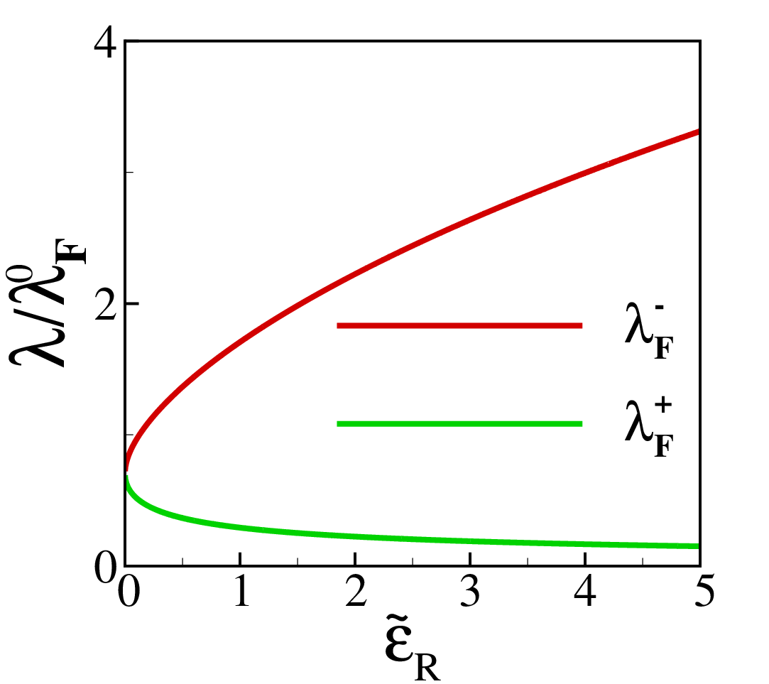
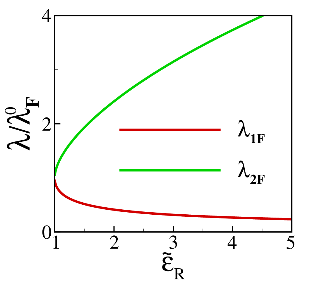
By solving this integral, we reach to two linear equations for the relaxation times $\tau^{+}$ and $\tau^{-}$ (not shown). In Fig. 6 (left panel), we have plotted the relaxation times obtained by ETTS method. The results of GRTA are also plotted for comparison. As it is seen, these two methods are completely consistent.

Modified relaxation time approximation (MRTA) is another method for solving the Boltzmann equation for isotropic 2DRSs. In this method, the relaxation time in the band $n$ is given by:

In both the ETTS and GRTA methods, we need to solve two coupled equations in order to obtain the relaxation times, while in the MRTA method band dependence of $\tau_{MRTA}$ is neglected. In Fig. 6 (right panel), we have plotted the relaxation times obtained by the MRTA. In the band $-$, due to the larger Fermi wavelength, we expect the relaxation time to be smaller, but in GRTA, because of the coupling between the two bands, the relaxation time $\tau^{-}$ is larger than the corresponding one in MRTA. Similarly, in the band $+$, because of the coupling with the band $-$, the relaxation time is smaller than the corresponding one in MRTA. Regardless of the differences in these methods, the behaviors of the relaxation times versus CMS are qualitatively the same. The same discussions are also valid when the Fermi energy is located below the BCP.

Below the BCP, the conductivity of the 2DRS is obtained as (see appendix B):

where $\tilde{\varepsilon}_{\rm R}=\varepsilon_{\rm R}/(2|\varepsilon_{\rm F}|)$. In the isotropic case, $\tau_{x}^{1}=\tau_{y}^{1}=\tau^{1}$ and $\tau_{x}^{2}=\tau_{y}^{2}=\tau^{2}$, and the conductivities along $x$ and $y$ directions are identically the same. In Fig. 9 (left panel), we have plotted the relaxation times $\tau^{1,2}$ versus $\tilde{\xi}$. Since the Fermi wavelength in the branch 1 is smaller than 2 (see Fig. 4), the relaxation time $\tau^{1}$ is always larger than $\tau^{2}$. The Fermi wavelength in the branch $\nu$ is given by $\lambda_{\nu{\rm F}}=\lambda_{\rm F}^{0}/[\sqrt{\tilde{\varepsilon}_{\rm R}}-(-1)^{\nu}\sqrt{\tilde{\varepsilon}_{\rm R}-1}]$. In Fig. 9 (right panel), we have also plotted the conductivity of the system versus $\tilde{\xi}$ for different strengths of SOC. Similar to the two-band case, by increasing $\tilde{\xi}$ the conductivity decreases rapidly, becomes minimum at $\tilde{\xi}_{min}\sim\lambda_{\rm F}^{av}/2\pi$, where $\lambda_{\rm F}^{av}=\lambda_{\rm F}^{0}/\sqrt{\tilde{\varepsilon}_{\rm R}}$, and then increases gradually. In contrast to the two-band case the conductivity decreases by decreasing the SOC and goes toward zero in the limit of $\tilde{\varepsilon}_{\rm R}\rightarrow 1$. Actually, by decreasing SOC number of electrons with the same $k$ ($k_{1{\rm F}}\approx k_{2{\rm F}}$) but opposite velocities are almost equal and consequently conductivity is zero. In contrast, above the BCP the velocities in the bands $+$ and $-$ are always in the same directions and the system possesses a non zero conductivity.

We presented a comprehensive study of the transport properties of 2DRSs with strong SOC doped with magnetic impurities interacting via an exchange interaction. Exchange interactions between magnetic impurities cause the formation of magnetic clusters which their mean sizes (CMSs) and number (CN) depend on temperature. Treating magnetic clusters as scattering centers, distributed randomly on the surface of the 2DRS, we modeled the interaction of itinerant electrons with magnetic clusters by a long-range scattering potential, and demonstrated that the combined effects of Rashba SOC and magnetic clusters cause the system to be anisotropic which the anisotropy strongly depends on both the clusters’ mean size and spin, the strength of SOC and the location of Fermi energy with respect to the BCP. Using semi-classical Boltzmann approach we computed the relaxation times, the conductivities and the AMRs of the system in both regimes of above and below the BCP. We demonstrated that: (i) In the isotropic case the conductivity is a non-monotonic function of CMS, it decreases by increasing CMS, becomes minimum at $\tilde{\xi}_{min.}$, and then increases by CMS. By increasing the strength of SOC the conductivity increases for all CMSs. (ii) In the anisotropic case, the AMR strongly depends on the CMS, it increases by increasing CMS and saturates to unit at large CMSs. Moreover, the angular dependence of the AMR is unconventional in comparison with the well-known $\cos^{2}\theta$ angular dependence seen in ferromagnets. For small CMSs, below the BCP the angular dependence of the AMR is consistent with 3D magnetic topological insulators. (iii) In contrast to the two-band regime in which the AMR always increases by increasing the strengths of SOC, in the single band regime it experiences a minimum at a $\tilde{\varepsilon}_{\rm R}$ which strongly depends on the CMS. For small CMSs, in the single band regime the AMR is almost constant and does not change by varying $\tilde{\varepsilon}_{\rm R}$, however in the two-band regime the AMR strongly depends on the strength of SOC even at small CMSs.

Both the CMS and CN depend on temperature. By knowing their temperature dependence, the temperature dependence of conductivities can be obtained which is crucial in investigation of the thermoelectric properties of the 2DRSs. The temperature dependences of the CMS and CN can be obtained using Monte Carlo simulations, which are left for future study.

References

- Rashba (1960) E. I. Rashba, Sov. Phys. Solid State 2, 1109 (1960).
- Vas’ko (1979) F. T. Vas’ko, JETP Lett. 30, 541 (1979).
- Bychkov and Rashba (1984) Y. A. Bychkov and E. I. Rashba, JETP Lett. 39, 78 (1984).
- Sharma (2005) P. Sharma, Science 307, 531 (2005), https://science.sciencemag.org/content/307/5709/531.full.pdf .
- Zutić et al. (2004) I. Zutić, J. Fabian, and S. Das Sarma, Rev. Mod. Phys. 76, 323 (2004).
- Cappelluti et al. (2007) E. Cappelluti, C. Grimaldi, and F. Marsiglio, Phys. Rev. Lett. 98, 167002 (2007).
- Grimaldi (2005) C. Grimaldi, Phys. Rev. B 72, 075307 (2005).
- Wu et al. (2014) L. Wu, J. Yang, S. Wang, P. Wei, J. Yang, W. Zhang, and L. Chen, Applied Physics Letters 105, 202115 (2014), https://doi.org/10.1063/1.4902134 .
- Xiao et al. (2016a) C. Xiao, D. Li, and Z. Ma, Phys. Rev. B 93, 075150 (2016a).
- Nunner et al. (2008) T. S. Nunner, G. Zaránd, and F. von Oppen, Phys. Rev. Lett. 100, 236602 (2008).
- vZitko and Bonvca (2011) R. vZitko and J. Bonvca, Phys. Rev. B 84, 193411 (2011).
- Zarea et al. (2012) M. Zarea, S. E. Ulloa, and N. Sandler, Phys. Rev. Lett. 108, 046601 (2012).
- Isaev et al. (2012) L. Isaev, D. F. Agterberg, and I. Vekhter, Phys. Rev. B 85, 081107 (2012).
- Yan et al. (2012) Z. B. Yan, X. S. Yang, L. Sun, and S. L. Wan, The European Physical Journal B 85, 417 (2012).
- Výborný et al. (2009) K. Výborný, A. A. Kovalev, J. Sinova, and T. Jungwirth, Phys. Rev. B 79, 045427 (2009).
- Walls et al. (2006) J. D. Walls, J. Huang, R. M. Westervelt, and E. J. Heller, Phys. Rev. B 73, 035325 (2006).
- Akabli et al. (2011) K. Akabli, Y. Magnin, M. Oko, I. Harada, and H. T. Diep, Phys. Rev. B 84, 024428 (2011).
- Akabli and Diep (2008) K. Akabli and H. T. Diep, Phys. Rev. B 77, 165433 (2008).
- Zarezad and Abouie (2018) A. N. Zarezad and J. Abouie, Phys. Rev. B 98, 155413 (2018).
- Ast et al. (2007) C. R. Ast, J. Henk, A. Ernst, L. Moreschini, M. C. Falub, D. Pacilé, P. Bruno, K. Kern, and M. Grioni, Phys. Rev. Lett. 98, 186807 (2007).
- Ast et al. (2008) C. R. Ast, D. Pacilé, L. Moreschini, M. C. Falub, M. Papagno, K. Kern, M. Grioni, J. Henk, A. Ernst, S. Ostanin, and P. Bruno, Phys. Rev. B 77, 081407 (2008).
- Moreschini et al. (2009) L. Moreschini, A. Bendounan, H. Bentmann, M. Assig, K. Kern, F. Reinert, J. Henk, C. R. Ast, and M. Grioni, Phys. Rev. B 80, 035438 (2009).
- Gierz et al. (2009) I. Gierz, T. Suzuki, E. Frantzeskakis, S. Pons, S. Ostanin, A. Ernst, J. Henk, M. Grioni, K. Kern, and C. R. Ast, Phys. Rev. Lett. 103, 046803 (2009).
- Ishizaka and et.al (2011) K. Ishizaka and et.al, Nature Materials. 10, 521–526 (2011).
- Eremeev et al. (2012) S. V. Eremeev, I. A. Nechaev, Y. M. Koroteev, P. M. Echenique, and E. V. Chulkov, Phys. Rev. Lett. 108, 246802 (2012).
- Eremeev et al. (2013) S. V. Eremeev, I. P. Rusinov, I. A. Nechaev, and E. V. Chulkov, New Journal of Physics 15, 075015 (2013).
- Landolt et al. (2012) G. Landolt, S. V. Eremeev, Y. M. Koroteev, B. Slomski, S. Muff, T. Neupert, M. Kobayashi, V. N. Strocov, T. Schmitt, Z. S. Aliev, M. B. Babanly, I. R. Amiraslanov, E. V. Chulkov, J. Osterwalder, and J. H. Dil, Phys. Rev. Lett. 109, 116403 (2012).
- Landolt et al. (2013) G. Landolt, S. V. Eremeev, O. E. Tereshchenko, S. Muff, B. Slomski, K. A. Kokh, M. Kobayashi, T. Schmitt, V. N. Strocov, J. Osterwalder, E. V. Chulkov, and J. H. Dil, New Journal of Physics 15, 085022 (2013).
- Crepaldi et al. (2012) A. Crepaldi, L. Moreschini, G. Autès, C. Tournier-Colletta, S. Moser, N. Virk, H. Berger, P. Bugnon, Y. J. Chang, K. Kern, A. Bostwick, E. Rotenberg, O. V. Yazyev, and M. Grioni, Phys. Rev. Lett. 109, 096803 (2012).
- Manchon and Zhang (2008) A. Manchon and S. Zhang, Phys. Rev. B 78, 212405 (2008).
- Liu and Xiong (2006) P. Liu and S.-J. Xiong, The European Physical Journal B - Condensed Matter and Complex Systems 51, 513 (2006).
- J.K. Furdyna (1988) J. K. E. J.K. Furdyna, Semiconductors and Semimetals (Academic Press, London, Vol. 25, 1988).
- Schliemann and Loss (2003) J. Schliemann and D. Loss, Phys. Rev. B 68, 165311 (2003).
- Trushin et al. (2009) M. Trushin, K. Výborný, P. Moraczewski, A. A. Kovalev, J. Schliemann, and T. Jungwirth, Phys. Rev. B 80, 134405 (2009).
- Xiao et al. (2016b) C. Xiao, D. Li, and Z. Ma, Frontiers of Physics 11, 117201 (2016b).
- Sinitsyn (2007) N. A. Sinitsyn, Journal of Physics: Condensed Matter 20, 023201 (2007).
- Fukuma et al. (2003) Y. Fukuma, H. Asada, N. Nishimura, and T. Koyanagi, Journal of Applied Physics 93, 4034 (2003), https://doi.org/10.1063/1.1555697 .
- Schulz et al. (2019) S. Schulz, I. Nechaev, M. Güttler, G. Poelchen, A. Generalov, S. Danzenbächer, A. Chikina, S. Seiro, K. Kliemt, A. Vyazovskaya, T. Kim, P. Dudin, E. Chulkov, C. Laubschat, E. Krasovskii, C. Geibel, C. Krellner, K. Kummer, and D. Vyalikh, npj Quantum Materials 4 (2019), 10.1038/s41535-019-0166-z.
- Sabzalipour et al. (2015) A. Sabzalipour, J. Abouie, and S. H. Abedinpour, Journal of Physics: Condensed Matter. 27, 115301 (2015).
- Tokura (1998) Y. Tokura, Phys. Rev. B 58, 7151 (1998).