=n_max=n_max=1.26em, framextopmargi2em, framexbottommargi2em, showspaces=false, showtabs=false, showstringspaces=false, frame=none, tabsize=4, stepnumber=1, basicstyle=, backgroundcolor=, breaklines=True, postbreak= ,
A versatile tool for cluster lensing source reconstruction. I. methodology and illustration on sources in the Hubble Frontier Field Cluster MACS J0717.5+3745 2020A versatile tool for cluster lensing source reconstruction. I. methodology and illustration on sources in the Hubble Frontier Field Cluster MACS J0717.5+3745--References
Abstract
We describe a general purpose method to reconstruct the intrinsic properties of sources lensed by the gravitational potential of foreground clusters of galaxies. The tool Lenstruction is implemented in the publicly available multi-purpose gravitational lensing software Lenstronomy, in order to provide an easy and fast solution to this common astrophysical problem. The tool is based on forward modeling the appearance of the source in the image plane, taking into account the distortion by lensing and the instrumental point spread function (PSF). For singly-imaged sources a global lens model in the format of the Hubble Frontier Fields (HFF) lensing maps is required as a starting point. For multiply-imaged sources, the tool can also fit and apply first (deflection), second (shear, convergence), and third order (flexion) corrections to the local gravitational potential to improve the reconstruction, depending on the quality of the data. We illustrate the performance and features of the code with two examples of multiply-imaged systems taken from the Hubble Frontier Fields, starting from five different publicly available cluster models. We find that, after our correction, the relative magnification - and other lensing properties - between the multiple images become robustly constrained. Furthermore, we find that scatter between models of the reconstructed source size and magnitude is reduced. The code and jupyter notebooks are publicly available.
Keywords:
galaxies:clusters:individual: MACS J0717.5+3745-- gravitational lensing: strong1 Introduction
Cluster of galaxies acts as the most powerful gravitational lenses, magnifying and distorting background distant sources. For a given instrumental setup, the magnification effect enables the study of sources with higher sensitivity and resolution, acting effectively as a cosmic telescope (Marshall et al. 2007, e.g.). Studying the background source helps to probe the galaxy formation and evolution including the morphology, size, kinematics, star formation history, and chemical abundances (Richard et al. 2006; Stark et al. 2008; Sharon et al. 2012; Jones et al. 2015; Bouwens et al. 2017; Kawamata et al. 2018; de La Vieuville et al. 2019). In addition, cluster lensing also contributes to understanding the mass distribution of clusters of galaxies, probing the dark matter, the geometry and absolute scale of the universe with measurement of the time delay between multiple images (Jullo et al. 2010; Hoekstra et al. 2013; Kelly et al. 2015; Natarajan et al. 2017; Caminha et al. 2017; Grillo et al. 2018; Birrer et al. 2019).
A necessary condition for exploiting scientifically the strong lensing effect is modeling the potential of the deflector. From a technical standpoint, lens modeling of both galaxy-scale and cluster-scale lenses presents a lot of challenges. For example, the mass sheet degeneracy is a concern in both cases (Seitz & Schneider 1997; Gorenstein et al. 1988), even though the presence of multiple families of multiple images at multiple redshifts can alleviate the concern in clusters (Bradač et al. 2004). Much progress has been achieved in the past twenty years, somehow leading to parallel and independent developments in cluster and galaxy-scale lensing.
In galaxy-scale lensing (see, e.g., Treu 2010, for a review), the number of image pixels that records information of the lensing system is generally of order , the deflector is often a dynamically relaxed massive galaxy that can be described by a relatively simple mass model, and there is one or at most two systems of multiple images. These features mean that one can use computationally fast mass models (Kormann et al. 1994, e.g., the singular isothermal ellipsoid (SIE)) and full image plane modeling is tractable with desktop computing power (Warren & Dye 2003; Treu & Koopmans 2004; Vegetti & Koopmans 2009; Tagore & Keeton 2014; Birrer et al. 2015; Nightingale & Dye 2015).
In contrast, in cluster-scale lensing (see, e.g., Kneib & Natarajan 2011, for a review), the lensing potential is often complex and multimodal, there are multiple systems of multiple images often at different redshifts, and the image can span almost a full Hubble Space Telescope image (- pixels), albeit sparsely. Therefore, whereas state of the art galaxy-scale lens models can handle a full source reconstruction, cluster lens models tend to focus on reproducing multiple image positions and do not work at the pixel level. A good example is provided by the Hubble Frontier Fields (HFF) lens modeling effort. In a game-changing effort, multiple map-making teams have made their lens models public 11 1 http://www.stsci.edu/hst/campaigns/frontier-fields/Lensing-Models. The models are based on hitherto unprecedented numbers of multiple images, including many with spectroscopic confirmation, and have been shown to generally provide good estimates of the mass distribution and magnification effect of the clusters. However, the lens model is constrained primarily by the positions of the lensed images (and sometimes weak lensing) and is not designed to do full source reconstruction on a sub-arcsecond scale (Sharon et al. 2012; Meneghetti et al. 2017). Furthermore, the lens-modeling teams contracted by HFF are independently using a variety algorithm resulting in differences between lens models. The performance of those algorithms has been investigated in the literature. For example, Acebron et al. 2017 and Meneghetti et al. 2017 compare the methods using simulated data, while Priewe et al. 2017 and Remolina González et al. 2018 carried out an evaluation of lens models of the HFF cluster. Those works have confirmed the accuracy and precision of the strong lensing methods applied, and showed that the major uncertainties in the lens models are found near cluster substructure and in the high magnification regions around the critical lines that are not immediately constrained by nearby multiple images.
Even for the most ambitious cluster-scale lens modeling projects, additional effort (Rau et al. 2014; Sharon & Johnson 2015, e.g.,) beyond image position fitting is needed if one wants to reconstruct a specific source in detail, and take full advantage of the quality of the data (Postman et al. 2012; Treu et al. 2015; Lotz et al. 2017, e.g.). The difficulty of reconstruction lies in achieving lens models that are sufficiently precise for source reconstruction up to sub-arcsecond scale, while allowing for enough freedom in the source light profiles and simultaneously dealing with blurring effect in the image plane. Also, the lens models often under-constrain the source-lens degeneracy for systems only observed in a single image.
In this paper, we introduce a general-purpose methodology to solve the problem of cluster-scale source reconstruction in a variety of contexts. Starting with an initial guess lens model, we adopt the forward modeling approach. In practice, to correct the initial lens model, we employ the perturbative method proposed by Blandford et al. 2001 and further studied by Koopmans 2005; Blandford et al. 2006; Suyu et al. 2009. The central concept is starting from a good global lens model, then performing the localized, small-scale potential perturbation near the particular images. To represent the wide range of source morphologies, we utilize a linear decomposition of the modeled source into a series of basis functions of different profiles. In addition, our approach uses the technology developed in the context of galaxy-scale lensing to deal with the blurring effect from the point spread function (PSF) (Treu & Koopmans 2004; Blandford et al. 2006).
Our approach is implemented in the code Lenstruction powered by Lenstronomy22 2 https://github.com/sibirrer/lenstronomy, a multi-purpose open-source gravitational lens modeling python package, which is developed by Birrer & Amara 2018, and based on the methodology outlined by Birrer et al. 2015. The scientific goal of Lenstruction is to allow scientists to study in detail source plane quantities like morphologies, sizes, luminosities, star formation rates, metallicities for large sample of objects in a self-consistent and practical way, also to explore systematic uncertainties related to the lens models. This need is driven by the increasing quality and quantity of cluster-lens data from current and future observatories, from the Hubble Frontier Fields to e.g., the already planned guaranteed time and Early Release Science programs on the James Webb Space Telescope. The software Lenstronomy at the core of Lenstruction has been applied successfully to diverse scientific problems, such as cosmographic analysis (Birrer et al. 2016; Birrer et al. 2019; Shajib et al. 2019), modeling lensed quasars (Shajib et al. 2018), probing dark matter structure (Birrer et al. 2017; Gilman et al. 2019), quasar host galaxy decompositon (Ding et al. 2019) and to generate simulations for a Convolutional Neural Network analysis (e.g. Diaz Rivero & Dvorkin 2019, Park et al. in prep, Wagner-Carena et al. in prep). A comparison with a different source reconstruction method by Joseph et al. 2019 is presented in their paper. We refer the reader to the GitHub repository for more general information about Lenstronomy.
Above applications are on the galaxy-scale regime but the same methods can be ported to the cluster regime. As a first illustration of Lenstruction, we apply it to two sets of multiple images in the Hubble Frontier cluster MACSJ0717.5+3745, starting from 5 different publicly available models. We show that relative lensing corrections are needed and substantially improve the agreement between the models.
The paper is organized as follows. In Section 2, we review the lens modeling technique. In Section 3, we introduce and describe the algorithm Lenstruction. In Section 4, we present two examples of source reconstruction of lensed images in the lensing cluster MACSJ0717.5+3745. We make comparison of relative morphology, magnification and source properties between HFF lens models in Section 5. Summary and conclusions are given in Section 6.
Lenstruction, together with documentation and example notebooks are publicly available 33 3 https://github.com/ylilan/lenstruction . The users are kindly requested to cite this paper, Birrer & Amara 2018, and Birrer et al. 2015, if they make use of Lenstruction.
2 Methodology
Lenstruction adopts a forward modeling approach to reconstruct source brightness distribution, simultaneously considering lensing and blurring effects, under a Bayesian inference formalism as described Section 2.1. We discuss the degeneracy between lensing operator and source light model, and potential correction on lensing operators in Section 2.2. The types of descriptions of the surface brightness distribution of the source currently implemented in Lenstruction are given in Section 2.3. The technique adopted to regularize model complexity is described in Section 2.4.
2.1 Forward modeling technique: source to image plane mapping
In a forward modeling approach, to reconstruct the source surface brightness, , from the data, , we first use a theoretical light profile of and predict the lensed image(s) as
| (1) |
where is the lensing operator, and is the PSF blurring operator that is determined by the property of the telescope. Following Birrer et al. 2015, for a given lensing operator, the scaling of surface brightness in the source results in a linear response of the model. We thus impose a set of basis function describing the source suface brightness, , with a vector of flux normalization coefficients, , such that the total source is a linear superposition of those basis set. The modeled image is then a linear superposition too with the response matrix such that the modeled image .
We employ Bayesian inference methods to estimate the posterior distribution function, , of the free parameters in the model. The log-likelihood function of the observed data given a model is,
| (2) |
where and are the observed and modeled flux in each pixel respectively, is the error in each pixel and is the total number of pixels in the modeled image. We estimate the error in each pixel as a combination of a Gaussian background rms, and a Poisson term scaled with the exposure time, , of each pixel, see details in Birrer et al. 2015 as
| (3) |
The best-fitting parameters of source light model is estimated by maximizing the posterior distribution function. The source configuration for a given lensing operator and basis set can be solved by a linear minimization problem:
| (4) |
where W is the weight matrix. In our case, treating noise as uncorrelated, is the diagonal matrix with . In practice, we utilize Weighted Least Square (WLS) method to reconstruct the source surface brightness.
To figure out the best-fit configuration of the source light model, we adopt two steps. First, we need to find a solution for a given lens and source model assumptions. Then, we change the choices of model complexity as long as changing and increasing complexity improves the results.
To simplify the problem, the effects of dust and the contamination by foreground lens light have been ignored in this paper. Taking dust and foreground light into account in the forward modeling is straightforward from a conceptual point of view and implemented in lenstronomy (Shajib et al. 2019, see e.g.).
2.2 Degeneracies and observational constraints on the lensing operator
2.2.1 Degeneracies
The unknown intrinsic source inherits a degeneracy with the lensing operator . As shown in Figure 1, let us assume that we observe image , and the initial guess of the lensing operator is . Given the data and the lensing operator, we can reconstruct the source . We can introduce any arbitrary correction operator provided that there exists a corresponding inverse with equals the unit operator to transform simultaneously the lensing operator and the source without any observable effect on the data as
| (5) |
Unless intrinsic knowledge of the source is assumed or available through other means, it is impossible to tell if the true source is or . The equation above effectively describes the most general lensing degeneracy of which the mass sheet transform (Falco et al. 1985) is the special case where is a scalar.
2.2.2 Constraints in multiply-imaged case
When multiple images are available of the same source, one can obtain information of the relative lensing operators, even though of course the absolute intrinsic source properties are mathematically unknown due to the degeneracy described in Section 2.2.1. In the case of two images as described in Figure 1, the two modeled lensed images of and are
| (6) |
Two images from the same source are related by the transformation operator mapping image 2 to image 1.
| (7) |
where is independent on a source distortion operator and the constraints on solely depends on the quality and information of the observations (Wagner 2019, see e.g.,). is the primary operator that needs to be sufficiently accurate to allow a simultaneous reconstruction of both images. If the initial lensing operator is insufficiently accurate, the WLS fails to reconstruct a source that matches both images simultaneously:
| (8) |
where i = 1, 2 for two images respectively and the norm simultaneously applied for the same coefficients on both images. Thus, in the case of multiple images, we can constrain the lensing operators based on information contained in the transformation matrix . For example, the magnification ratio predicted by lensing operators is intuitively well constrained by the observed images. In practice, the amount of corrections to be applied to the initial lensing operators depend on the quality of the data. In this work we restrict ourselves to third order polynomial perturbations of the lensing potential, which are sufficient for the vast majority of sources behind cosmic telescopes that do not suffer from extreme distortion. Correction to higher-order are needed for highly distorted sources. If the highly distorted feature appears in comparison of multiple lensed images, higher order lensing effect can be constrained using a more general approach departing from a Taylor series expansion in the lensing potential (see details in Birrer 2020, in preparation).
2.3 Model surface brightness distribution of the source
In our approach, the source surface brightness distribution is a linear combination of a set of simple models. To describe a wide range of unknown background astronomical sources with a finite sets, we make use of elliptical Sérsic (Sersic 1968) and the two-dimensional Cartesian shapelets (Refregier 2003) 44 4 Lenstronomy supports a variety of non-linear profiles, and Lenstruction allows for the full support of the available functionality of Lenstronomy . Shapelets are given by:
| (9) |
where is a characteristic scale, and are one-dimensional Cartesian shapelet, as:
| (10) |
where is the order of , the Hermite polynomial. The order determines numbers of basis sets m by . As the order increases, one can capture more complexity in the source surface brightness profile. The characteristic scale is typically about the size of the source. The minimum and maximum scales being resolved up to order are given by and .
2.4 Model complexity regularization
For a given model complexity, the source is reconstructed via linear minimization. We then repeat the procedure while varying model complexity, and we employ the Bayesian information criterion (BIC) method to balance goodness of fit and model complexity simultaneously following Birrer et al. 2019. BIC is computed as
| (11) |
where and are the number of data points and free parameters within the model respectively, and is the maximum likelihood value given the model. Usually, the likelihood increases with the source light model complexity. However, the number of free parameters also increases, and the minimum BIC criterion balances the increase in source complexity with the additional parameters in order to avoid over-fitting the data.
3 Overview of Lenstruction
To facilitate the forward modeling approach described in Section 2 and its applicability in the cluster regime on real data to the broader community, we develop the python package Lenstruction build on top of Lenstronomy. Lenstronomy provides the core functionalities of the modeling and fitting described in Section 2 and is the work horse underneath through which those tasks are executed. Lenstruction is the layer on top that provides the interface to the specific cluster data products and executes the specific tasks required to achieve reliable source reconstructions and lens model corrections in the cluster lensing regime.
Lenstruction contains several independent modules. The core module of Lenstruction is ClsrWorkflow (Cluster lensing source reconstruction Workflow). ClsrWorkflow inherits the Workflow module of Lenstronomy (Birrer & Amara 2018) tailored for perturbative lens modeling and source reconstruction in the cluster context and manages fitting and sampling routines as described in Section 3.2. The linear minimization, exploration of parameters space, and model complexity regularization are all performed through this module. The other modules are described in detail in Section 3.1. The DataProcess module configures the imaging data to be modeled by the ClsrWorkflow. The LensSpecify module handles the configuration of the lens model and the SourceSpecify module handles the configuration of the source model to be passed into the core Lenstronomy modules. Lenstruction inherits conventions and many functionalities from Lenstronomy and allows to keep up with the development of the broader Lenstronomy ecosystem.
3.1 Configuration of the data and model setup
The DataProcess module manages and facilitates the retrieval of the relevant information of the lensed images from the data, such as the blurring operator, known in astronomy as the point spread function (PSF), positional information and the coordinate system, pixel size, exposure time and noise, and casts those quantities into the conventions used by Lenstronomy. The identification of lensed image makes use of and in package (Bradley et al. 2019) 55 5 https://photutils.readthedocs.io/en/stable/index.html. For the PSF, both pixelized convolution kernels, as well as analytic profiles, are supported through Lenstronomy. This is a clear step forward with respect to most previous work on extended images in cluster lensing, in which the blurring effect is often ignored.
The LensSpecify module defines the parameterization of the lensing operators and sets up the fitting configuration. In the current implementation, we assume that the lens potential is approximately smooth over the area spanned by each observed image. Thus, the initial shear and convergence are taken directly from the convergence and shear maps provided in the input setting. Higher-order flexion terms can also be initialized when required. The default flexion terms are set to zero, assuming that the initial model is insufficiently accurate to provide valid initial guesses.
Users can specify the parameters to be held fixed, and assign bounds and priors to the free parameters during the modeling procedure.
The SourceSpecify module provides the functionality to describe the surface brightness in the source plane with various analytic profiles as well as representations in shapelet basis sets in conjunction with the Lenstronomy LightModel module. The superposition of profiles is allowed, and the user can choose whether the constraints of the independent profile types are connected or not.
3.2 Modeling management
The ClsrWorkflow module is designed to model a wide range of source and lens model complexities in the cluster environment.
The ClsrWorkflow module operates, as shown in Figure 2. It starts with the lowest model complexity, and default setting is elliptical for source light model and lensing parameters up to convergence and shear. For a given lensing operator and source brightness distribution, it then solves for the source parameters via linear minimization, see details in Equation 4. Changes in lensing operator and/or source brightness distribution, however, require solving a nonlinear problem. This step is performed by a Particle Swarm Optimization (PSO) (Kennedy & Eberhart 1995). PSO optimizes a candidate solution by employing particles to the explore parameter volume. The particles are expected to swarm toward the best solution. The use of multiple particles is aimed at avoiding local maxima as it is often the case of optimizers starting from a single point.
If the adopted models can not produce an acceptable fit of the data, the module increases the model complexity. Higher-order lensing corrections or shapelets are included and the fitting is repeated. The process is repeated until the minimum BIC is reached. Once the minimum BIC solution is found, one can run a more time-consuming Markov chain Monte Carlo (MCMC) process to explore the full posterior and provide confidence intervals as well as degeneracies among model parameters (Foreman-Mackey et al. 2013, using emcee).
4 Examples: analysis of two multiply-imaged systems in the lensing cluster MACSJ0717.5+3745
As an illustration of Lenstruction and to demonstrate the power of the modules and their underlying algorithm on a real and complex example, we present source plane reconstruction of two multiply-imaged sources in one of the HFF cluster MACSJ0717.5+3745 (Ebeling et al. 2014) at redshift . The pre-processing of the images and set-up of model configurations are illustrated in Section 4.1. Lenstruction is applicable for both singly- and multiply- imaged sources. We present the details of reconstruction Section 4.2.
4.1 Data and model configuration
Hubble Space Telescope images (through filter F435W) of two multiply-imaged sets are shown in Figure 3. Coordinates are listed in Table 1. For consistency with previous work, we keep the same IDs of the two systems (3 and 4) as in the paper by Schmidt et al. 2014. The DataProcess module can deblend multiple images from potential foreground contamination, as shown in Figure 4. For this example, a bright star with coordinate (RA, Dec) = (109.3778185, 37.75322111) is selected as the fiducial PSF.

| ID | RA | DEC | redshift |
|---|---|---|---|
| 3.1 | 109.398545 | 37.741498 | 1.855 |
| 3.2 | 109.394459 | 37.739172 | 1.855 |
| 3.3 | 109.407156 | 37.753831 | 1.855 |
| 4.1 | 109.381093 | 37.750440 | 1.855 |
| 4.2 | 109.376338 | 37.744602 | 1.855 |
| 4.3 | 109.391097 | 37.763077 | 1.855 |

We adopt lens models from five independent teams contracted by HFF, Bradač, Williams, CATS, Zitrin, and Sharon (Bradač et al. 2005; Bradač et al. 2009; Sebesta et al. 2016; Liesenborgs et al. 2007; Limousin et al. 2016; Zitrin et al. 2015; Johnson et al. 2014), to initialize LensSpecify modules. Table 2 provides a summary of the models. Values of shear, convergence are reported in Table 3 and Table 5 for two lensed systems respectively.
| Model | Version | Method |
|---|---|---|
| Brada | v1 | Pixellated |
| Williams | v4.1 | Pixellated |
| CATS | v4.1 | Simply-parametrized |
| Zitrin-ltm | v1 | Simply-parametrized |
| Sharon | v4 | Simply-parametrized |
4.2 Description of modeling procedure
We now describe in detail the ClsrWorkflow module for the two real multiply-imaged case studies. We first show results starting from the Bradač model, then the comparison to the outcome using a different model as initialization is given in Section 5.1.
4.2.1 Modeling details of the multiply-imaged system 3
To start with a simpler problem, we consider each lensed image within multiply-imaged system 3 as an individual singly-imaged source, i.e., doing the source reconstruction independently, not demanding a joint source morphology. The morphologies of the observed images are compact, thus we just apply the lowest model complexity, an elliptical Sérsic profile for source, convergence and shear for the lens model. The singly-imaged system lacks the information required to constrain the lensing operator see details in Section 2.2.1, so we fix the lens parameters after initialization. We present the sources reconstructed from each image in Figure 5, while fitting results of this exercise are in Table 3.
For a multiply-imaged system, observed multiple images provide information to constrain the relative lensing operator (see details in Section 2.2.2). Before correcting the lens model, we present the results obtained using the uncorrected lens model for the combined reconstruction of the multiple images. As shown in Figure 6, the uncorrected lens model leads to poor results. The initial lens model is not sufficiently accurate to match all images simultaneously at the pixel level and needs corrections as expected. As only relative lens parameters can be constrained, letting all lensing operators free will unavoidably lead to degeneracies. To avoid this pitfall, we fix the lens parameters of the least magnified image (image 3.3 is the least magnified evaluated from Bradač team, see Table 3) to the value estimated by the global model. It is important to use the least magnified image because the uncertainties of magnification are proportional to magnification itself (Meneghetti et al. 2017). Also, the current implementation of our code only applies corrections up to flexion, and therefore it is best to take the least distorted image as reference. The full underlying degeneracy inherent in lensing can then be reconstructed analytically from the reconstruction and posteriors.
MCMC explores the full posterior and provides confidence intervals as well as degeneracies between parameters. As an example, we present the MCMC results of multiply-imaged source 3 with corrections applied to the initial lens model by the Bradač team in Figure 9. The first six histograms show constrained lensing operators of image 3.1 and 3.2 while image 3.3 is fixed. The uncertainty of the source parameters is shown in the remaining histograms.
Singly-imaged cases with uncorrected lens parameters


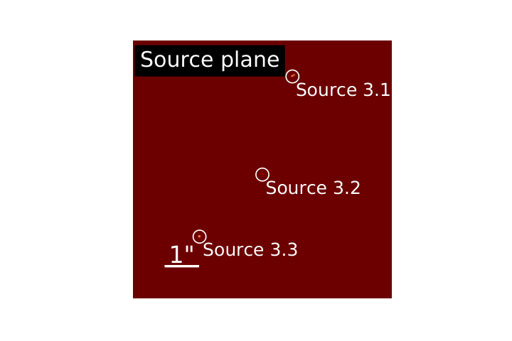
Multiply-imaged system 3 with uncorrected lens parameters


Multiply-imaged system 3 with corrected lens parameters


4.2.2 Modeling details of the multiply-imaged system 4
Images of system 4 are extended and complex, providing more information to constrain the model. Thus, we can explore the higher model complexity. We propose lens model up to flexion and source model with additional shapelet order . Image 4.3 is the least magnified estimated by Brada model, see Table 5, so we fix its lens parameters. We run a PSO and record the BIC value for regularization in Table 6. As we increase complexity, reduced and BIC decrease, indicating that the additional complexity is required. Next, we apply additional shapelet bases sequentially. The BIC reaches the lowest value (28 shapelet coefficients). We identified the nmax range with preliminary tests; BIC does not decrease significantly beyond 6, indicating that a higher level of source complexity are not required for this system. The results are shown in Figure 8. Each image in system 4 can also be treated as a singly-imaged case, as summarized in Table 5.
Multiply-imaged system 4 with corrected lens parameters


5 Comparison between models
Uncertainties in the lens model are a well-known source of systematic uncertainty in the use of clusters as cosmic telescopes. One of the goals of Lenstruction is to allow the wholesale investigation of this kind of uncertainty in a broad variety of contexts. As a primary illustration of the effects of the choice of lens model, that is used to fix the lens parameters of the least magnified image as well as the improvement introduced by Lenstruction in the relative distortions, we compare the reconstructed sources morphologies among different lens models in Section 5.1, and compute how they affect the source magnitude and effective radius for system 4 in Section 5.2. Then, in Section 5.3 we quantify how well the lensing operator is constrained by our procedure in the case of multiple images.
In this section, the two systems are considered as multiply-imaged, and corrections are applied to the initial lens models.
5.1 Morphological comparison
Considering lens models from different teams, we perform similar steps as for the Bradač model for the two multiply-imaged systems 3 and 4. The initial magnifications at the position of images among different models span a range of a factor of a few with some prominent outliers. For example, the magnifications predicted by the Williams model for system 3 differ up to an order of magnitude from the other ones. We also fix the lens parameters of the least magnified image evaluated from the corresponding team, while the others are free. For unbiased comparison between the performance of different lens models, we keep the same range of model complexity as for the Bradač model. Table 4 and Table 6 show the fitting results of multiply-imaged systems 3 and 4. While comparing Table 3 and Table 4, it should be noted that the lens parameters of the least magnified image 3.3 are kept fixed. While comparing Table 5 and Table 6, it should be noted that Image 4.3 is the fixed one for CATS, Zitrin-lmt, and Sharon teams, while image 4.2 is the least magnified image from the Williams models. Corrections to the free parameters are expected, owing to the information supplied by the extended images. For example, the data show that the magnification ratios are approximately a factor of a few. In contrast, the magnification ratios estimated via initial lens models between images are far larger, underscoring the need for a correction.
We present the comparison of reconstructed sources from five teams for the two systems in the bottom panels of Figure 7 and Figure 8, respectively. From left to right, the starting lens models are from Brada, Williams, CATS, Zitrin-lmt, and Sharon teams respectively. We clearly see differences in the morphology of the source according to the selected initial lens model. In order to quantify the effect on observables, we discuss how the magnitude and half-light radius depend on the estimate of the fixed least magnified image among the different models in Section 5.2.
and half-light radii of sources reconstructed from image 3.1, 3.2 and 3.3 respectively. Lens Team , , (AB) Brada (0.43, -0.19, 0.94), (0.15, -0.11, 0.69), (-0.10, 0.22, 0.38) -4.60, 16.26, 3.07 (26.60, 28.03, 26.40) (0.015, 0.008, 0.008) Williams (0.08, 0.19, 0.74), (0.07, 0.25, 0.75), (-0.27, -0.17, 0.58) 39.84, -204.08, 13.40 (..., .., 27.88) (..., ..., 0.006) CATS (0.29, -0.21, 0.75), (0.07, -0.13, 0.65), (-0.15, 0.22, 0.47) -12.53, 9.93, 4.76 (27.66, 27.55, 26.86) (0.011, 0.010, 0.007) Zitrin-lmt (0.19, -0.27, 0.77), (0.08, -0.19, 0.68), (-0.11, 0.15, 0.58) -17.83, 16.69, 7.05 (28.14, 28.07, 27.30) (0.008, 0.008, 0.005) Sharon (0.06, -0.32, 0.94), (0.06, -0.14, 0.76), (-0.23, 0.14, 0.50) -9.77, 29.07, 5.63 (27.41, 28.64, 27.07) (0.010, 0.006, 0.006)
| Lens Team | Models | BIC | , , | (AB) | |||
|---|---|---|---|---|---|---|---|
| Brada | , ES | 1.94 | 5673.78 | (0.17, -0.42, 0.87), (0.13, -0.08, 0.54), (-0.10, 0.22, 0.38) | -5.31, 5.31, 3.07 | 26.89 | 0.016 |
| Williams | , ES | 1.33 | 3935.58 | (-0.17, -0.25, 0.63), (-0.14, -0.21, 0.67), (-0.27, -0.17, 0.58) | 21.98, 22.12, 13.40 | 28.42 | 0.011 |
| CATS | , ES | 1.81 | 5288.12 | (0.11, -0.33, 0.94), (0.07, -0.03, 0.65), (-0.15, 0.22, 0.47) | -8.52, 8.57, 4.76 | 27.39 | 0.013 |
| Zitrin-lmt | , ES | 1.80 | 5237.08 | (0.09, -0.27, 0.93), (0.07, -0.04, 0.71), (-0.11, 0.15, 0.58) | -13.14, 12.89, 7.05 | 27.82 | 0.011 |
| Sharon | , ES | 1.54 | 4531.69 | (0.09, -0.31, 0.93), (0.06, -0.04, 0.67), (-0.23, 0.14, 0.50) | -10.07, 9.64, 5.63 | 27.57 | 0.012 |
| Lens Team | , , | (AB) | ||
|---|---|---|---|---|
| Brada | (-0.02, -0.57, 0.74), (-0.20, -0.15, 0.59), (0.06, -0.02, 0.40) | -3.88, 9.47, 2.81 | (26.83, 27.25, 26.92) | (0.062, 0.062, 0.072) |
| Williams | (-0.22, 0.42, 0.88), ( -0.11, -0.02, 0.29), (0.00, 0.06, 0.41) | -4.75, 2.03, 2.90 | (27.07, 26.54, 27.07) | (0.072, 0.073, 0.072) |
| CATS | ( -0.08 , -0.50 , 0.65), ( -0.12, -0.11, 0.34), (0.03, -0.03, 0.36) | -7.47, 2.46, 2.45 | (26.86, 26.61, 27.04) | (0.067, 0.076, 0.068) |
| Zitrin-ltm | (-0.08, -0.39, 0.76), (-0.17, -0.10, 0.55), (0.05, -0.10, 0.43) | -9.91, 6.11, 3.20 | (27.05, 26.98, 26.90) | (0.061, 0.069, 0.069) |
| Sharon | (-0.14, -0.44, 0.83), (-0.19, -0.09, 0.46), (0.09, -0.08, 0.46), | -5.43, 4.04, 3.61 | (26.77, 26.76, 26.87) | (0.068, 0.067, 0.071) |
| Lens Team | Models | BIC | , , | (AB) | |||
|---|---|---|---|---|---|---|---|
| Brada | , ES | 2.30 | 45615.73 | (-0.11, -0.36, 0.83), (-0.17, 0.06, 0.45),(0.06, -0.02, 0.40) | -8.87, 3.70, 2.81 | 26.11 | 0.12 |
| , ES | 2.03 | 40440.53 | (-0.10, -0.36, 0.83), (-0.16, 0.08, 0.46),(0.06, -0.02, 0.40) | -9.03, 3.85, 2.81 | 26.10 | 0.12 | |
| , ES, 2 | 1.65 | 32910.90 | (-0.14, -0.37, 0.73), (-0.15, -0.07, 0.51),(0.06, -0.02, 0.40) | -11.96, 4.70, 2.81 | 26.24 | 0.10 | |
| , ES, 4 | 1.55 | 31110.69 | (-0.13, -0.38, 0.74), (-0.19, -0.05, 0.48),(0.06, -0.02, 0.40) | -10.67, 4.31, 2.81 | 26.24 | 0.11 | |
| , ES, 6 | 1.50 | 30175.62 | (-0.12, -0.36, 0.75), (-0.19, -0.04, 0.49),(0.06, -0.02, 0.40) | -12.27, 4.50, 2.81 | 26.30 | 0.11 | |
| Williams | , ES | 2.65 | 52584.85 | (0.28, 0.25, 1.59), (-0.11, -0.02, 0.29),(0.23, -0.13, 0.15) | 4.83, 2.03, 1.53 | 25.48 | 0.14 |
| , ES | 2.30 | 45642.70 | (0.24, 0.24, 1.57), (-0.11, -0.02, 0.29),(0.19, -0.14, 0.18) | 4.77, 2.03, 1.62 | 25.45 | 0.14 | |
| , ES, 2 | 1.86 | 37152.67 | (0.24, 0.28, 1.57), (-0.11, -0.02, 0.29),(0.20, -0.17, 0.18) | 5.29, 2.03, 1.66 | 25.49 | 0.14 | |
| , ES, 4 | 1.77 | 35279.24 | (0.24, 0.28, 1.58), (-0.11, -0.02, 0.29),(0.21, -0.17, 0.17) | 4.99, 2.03, 1.62 | 25.48 | 0.14 | |
| , ES, 6 | 1.70 | 34153.55 | (0.24, 0.29, 1.59), (-0.11, -0.02, 0.29),(0.20, -0.19, 0.16) | 4.84, 2.03, 1.59 | 25.48 | 0.14 | |
| CATS | , ES | 2.30 | 45563.37 | (-0.10, -0.39, 0.82), (-0.23, 0.06, 0.39),(0.03, -0.03, 0.36) | -7.71, 3.17, 2.45 | 25.94 | 0.13 |
| , ES | 2.02 | 40338.54 | (-0.08, -0.39, 0.84), (-0.26, 0.08, 0.38),(0.03, -0.03, 0.36) | -7.52, 3.22, 2.45 | 25.92 | 0.13 | |
| , ES, 2 | 1.66 | 33109.41 | (-0.14, -0.39, 0.72), (-0.20, -0.07, 0.46),(0.03, -0.03, 0.36) | -10.72, 4.05, 2.45 | 26.08 | 0.11 | |
| , ES, 4 | 1.56 | 31312.44 | (-0.13, -0.40, 0.72), (-0.21, -0.06, 0.45),(0.03, -0.03, 0.36) | -10.15, 3.92, 2.45 | 26.10 | 0.12 | |
| , ES, 6 | 1.51 | 30266.73 | (-0.12, -0.39, 0.74), (-0.22, -0.05, 0.45),(0.03, -0.03, 0.36) | -10.11, 3.97, 2.45 | 26.14 | 0.12 | |
| Zitrin-ltm | , ES | 2.30 | 45608.29 | (-0.11, -0.37, 0.78), (-0.21, -0.02, 0.47),(0.05, -0.10, 0.43) | -9.94, 4.23, 3.20 | 26.23 | 0.11 |
| , ES | 2.03 | 40490.77 | (-0.10, -0.38, 0.77), (-0.22, -0.00, 0.44),(0.05, -0.10, 0.43) | -9.85, 3.77, 3.20 | 26.14 | 0.11 | |
| , ES, 2 | 1.65 | 32925.93 | (-0.14, -0.37, 0.71), (-0.17, -0.09, 0.54),(0.05, -0.10, 0.43) | -13.81, 5.73, 3.20 | 26.42 | 0.09 | |
| , ES, 4 | 1.55 | 31047.41 | (-0.13, -0.39, 0.70), (-0.20, -0.10, 0.49),(0.05, -0.10, 0.43) | -12.66, 4.76, 3.20 | 26.38 | 0.09 | |
| , ES, 6 | 1.51 | 30287.42 | (-0.12, -0.37, 0.72), (-0.22, -0.10, 0.50),(0.05, -0.10, 0.43) | -13.72, 5.22, 3.20 | 26.46 | 0.09 | |
| Sharon | , ES | 2.30 | 45743.04 | (-0.12, -0.32, 0.81), (-0.13, 0.00, 0.54),(0.09, -0.08, 0.46) | -12.39, 5.14, 3.61 | 26.46 | 0.09 |
| , ES | 2.05 | 40777.80 | (-0.11, -0.35, 0.80), (-0.17, -0.00, 0.50),(0.09, -0.08, 0.46) | -10.57, 4.52, 3.61 | 26.32 | 0.09 | |
| , ES, 2 | 1.64 | 32679.63 | (-0.13, -0.34, 0.73), (-0.14, -0.08, 0.57),(0.09, -0.08, 0.46) | -16.78, 6.29, 3.61 | 26.53 | 0.08 | |
| , ES, 4 | 1.54 | 30757.36 | (-0.12, -0.35, 0.74), (-0.18, -0.06, 0.53),(0.09, -0.08, 0.46) | -14.43, 5.41, 3.61 | 26.53 | 0.09 | |
| , ES, 6 | 1.50 | 30130.48 | (-0.12, -0.34, 0.74), (-0.19, -0.07, 0.54),(0.09, -0.08, 0.46) | -16.03, 5.86, 3.61 | 26.58 | 0.09 | |
5.2 Comparison of inferred source magnitude and size
The AB Magnitude in source plane is defined in a standard manner as,
| (12) |
where we adopt as zero-point for ACS F435W 25.673. The half-light radius is defined as the circular aperture that contains half light. We present the source plane magnitude and distribution of two systems in Figure 10. Each color represents the result for one of the five lens models. Numerical values can be found in Table 4 and Table 6. The upper two panels show the distribution of the magnitude and half-light radius for source 3, respectively. The source magnitude and span 1.5 magnitudes and 0.01", respectively. The bottom left panel shows how the magnitude of source 4 depends on modeling choices. During the modeling process, the lens parameters of the least magnified image were kept fixed as initial value acquired from each lens model. The source magnitude spans a range of about 1 magnitudes, with r.m.s. scatter 0.39 mags. The reconstructed source from the Sharon model is the faintest, while the one from the Williams model is the brightest. Overall, the magnitude is stable for each model, especially after additional model complexity by adding shapelet modes. The bottom right panel shows as a function of model complexity. The scatter in across models is approximately 18%, while the scatter of the least magnification, i.e., magnifications of the image 4.3, is approximately 25%. This dispersion suggests that the differences are fundamentally due to the mass-sheet degeneracy, and higher-order corrections may be required to improve the agreement between the models further.
5.3 Comparison of magnification ratio between lensed images
The relative magnification of the images is expected to be tightly constrained by the data. We show relative magnifications as a function of model complexity for each initial lens model in Figure 11, color coded as in Figure 10. It is clear that the initial estimates of differ dramatically for each lens model (see also Table 3.) For example, of image 3.2 varies from to . The discrepancy is not as dramatic for the absolute value of the relative magnifications, although it is still quite substantial.
After applying corrections to the initial lens models, we observe a definite improvement in the consistency of the magnification ratio. In Figure 11, the absolute values of relative and get close to . In those two cases, the parity is not well determined (hence the plus/minus dichotomy) because the image does not have much structure perpendicular to the highly stretched direction. The ratios and are well constrained to and , even though the initial models had substantial scatter.
6 Summary and Conclusion
From the perspective of lens modeling, cluster-scale lensing is full of challenges. Most state-of-the-art models are constrained exclusively by the positions of the lensed images rather than via extended source reconstruction. Therefore, additional efforts are needed to reconstruct the background source and determine the uncertainties associated with the lens model. Manually, performing source reconstruction on a handful of data is feasible. However, with current and upcoming observations, the quality and quantity of cluster lensing data are expected to improve dramatically.
In order to prepare for such an explosion of data, we have developed and made public a fast and versatile tool Lenstruction . It adopts a forward modeling approach to perform source reconstruction with corrections on the initial lens parameters, taking into account the blurring of the PSF. Lenstruction is implemented in python, building on the publicly available code lenstronomy.
In this paper, we describe the current implementation of Lenstruction as well as present the first illustration of its capabilities using two sets of multiple images in the HFF cluster MACS0717+3745, starting from five publicly available models as the initial guess of the lensing potential. One system is chosen to be of a compact source, providing limited information to correct the lens model. The other system is significantly extended and enables exploration of complexity, including corrections up to flexion order in the lens model and up to Sérsic + shapelets (with up to 6) in the source model.
We find that the choice of initial lens model with the lens model at the least magnified image held fixed affects the inferred source magnitude and size at the level of 0.39 mag and 18% r.m.s. scatter respectively. The scatter does not reduce by increasing the complexity of corrections on the lens model within the range considered in this work.
In contrast, the absolute ratio of magnifications between the images converges rapidly to a common value, even though the initial lens models provided sometimes dramatically different estimates.
In conclusion, we observe that our correction scheme produces a substantial improvement in the relative magnification, i.e., the quantity directly constrained by the data. Starting with significantly different initial models, the correction schemes makes them all converge to very similar absolute magnification ratios. The convergence is significantly more pronounced than observation in the case of magnitudes and effective radii, which are absolute quantities, and thus their measurement depends on breaking the mass sheet degeneracy.
In the future, we plan to carry out a similar investigation for a large sample of objects. The ultimate goal is measuring the irreducible scatter of current state of the art lens models as a way to quantify this source of systematic uncertainty in the estimation of the size luminosity/mass relation, and other observables, through cosmic telescopes (Yang et al. 2020, in preparation).
Acknowledgements
This work utilizes gravitational lensing models produced by PIs Bradač, Natarajan & Kneib (CATS), Merten & Zitrin, Sharon, Williams, Keeton, Bernstein and Diego, and the GLAFIC group. This lens modeling was partially funded by the HST Frontier Fields program conducted by STScI. STScI is operated by the Association of Universities for Research in Astronomy, Inc. under NASA contract NAS 5-26555. The lens models were obtained from the Mikulski Archive for Space Telescopes (MAST). LY, SB and TT acknowledge support from NASA through grant HST-GO-14630. LY is supported from the China Scholarship Council. TT acknowledges support by NASA through grant number JWST-ERS-01324.001 " Through the looking GLASS: a JWST exploration of Galaxy Formation and Evolution from Cosmic Dawn to Present Day’’ from the Space Telescope Science Institute, which is operated by AURA, Inc., under NASA contract NAS 5-26555. The authors thank Maruša Bradač, Xuheng Ding, Austin Hoag, Anowar J. Shajib, Guido Roberts-Borsani, and Jenny Wagner for several discussions that helped shaped the code and manuscript.
References
- Acebron et al. (2017) Acebron A., Jullo E., Limousin M., Tilquin A., Giocoli C., Jauzac M., Mahler G., Richard J., 2017, Monthly Notices of the Royal Astronomical Society, 470, 1809
- Birrer & Amara (2018) Birrer S., Amara A., 2018, Physics of the Dark Universe, 22, 189
- Birrer et al. (2015) Birrer S., Amara A., Refregier A., 2015, ApJ, 813, 102
- Birrer et al. (2016) Birrer S., Amara A., Refregier A., 2016, J. Cosmology Astropart. Phys., 2016, 020
- Birrer et al. (2017) Birrer S., Amara A., Refregier A., 2017, J. Cosmology Astropart. Phys., 2017, 037
- Birrer et al. (2019) Birrer S., et al., 2019, MNRAS, 484, 4726
- Blandford et al. (2001) Blandford R., Surpi G., Kundić T., 2001, in Brainerd T. G., Kochanek C. S., eds, Astronomical Society of the Pacific Conference Series Vol. 237, Gravitational Lensing: Recent Progress and Future Go. p. 65 (arXiv:astro-ph/0001496)
- Blandford et al. (2006) Blandford R. D., Suyu S. H., Marshall P. J., Hobson M. P., 2006, Monthly Notices of the Royal Astronomical Society, 371, 983
- Bouwens et al. (2017) Bouwens R. J., Illingworth G. D., Oesch P. A., Atek H., Lam D., Stefanon M., 2017, ApJ, 843, 41
- Bradač et al. (2005) Bradač M., Schneider P., Lombardi M., Erben T., 2005, A&A, 437, 39
- Bradač et al. (2009) Bradač M., et al., 2009, ApJ, 706, 1201
- Bradač et al. (2004) Bradač M., Lombardi M., Schneider P., 2004, A&A, 424, 13
- Bradley et al. (2019) Bradley L., et al., 2019, astropy/photutils: v0.7, doi:10.5281/zenodo.2533376, https://doi.org/10.5281/zenodo.2533376
- Caminha et al. (2017) Caminha G. B., et al., 2017, A&A, 607, A93
- Diaz Rivero & Dvorkin (2019) Diaz Rivero A., Dvorkin C., 2019, arXiv e-prints, p. arXiv:1910.00015
- Ding et al. (2019) Ding X., et al., 2019, arXiv e-prints, p. arXiv:1910.11875
- Ebeling et al. (2014) Ebeling H., Ma C.-J., Barrett E., 2014, ApJS, 211, 21
- Falco et al. (1985) Falco E. E., Gorenstein M. V., Shapiro I. I., 1985, ApJ, 289, L1
- Foreman-Mackey et al. (2013) Foreman-Mackey D., Hogg D. W., Lang D., Goodman J., 2013, PASP, 125, 306
- Gilman et al. (2019) Gilman D., Birrer S., Treu T., Nierenberg A., Benson A., 2019, Monthly Notices of the Royal Astronomical Society, 487, 5721
- Gorenstein et al. (1988) Gorenstein M. V., Falco E. E., Shapiro I. I., 1988, ApJ, 327, 693
- Grillo et al. (2018) Grillo C., et al., 2018, ApJ, 860, 94
- Hoekstra et al. (2013) Hoekstra H., Bartelmann M., Dahle H., Israel H., Limousin M., Meneghetti M., 2013, Space Science Reviews, 177, 75
- Johnson et al. (2014) Johnson T. L., Sharon K., Bayliss M. B., Gladders M. D., Coe D., Ebeling H., 2014, ApJ, 797, 48
- Jones et al. (2015) Jones T., et al., 2015, AJ, 149, 107
- Joseph et al. (2019) Joseph R., Courbin F., Starck J. L., Birrer S., 2019, A&A, 623, A14
- Jullo et al. (2010) Jullo E., Natarajan P., Kneib J. P., D’Aloisio A., Limousin M., Richard J., Schimd C., 2010, Science, 329, 924
- Kawamata et al. (2018) Kawamata R., Ishigaki M., Shimasaku K., Oguri M., Ouchi M., Tanigawa S., 2018, ApJ, 855, 4
- Kelly et al. (2015) Kelly P. L., et al., 2015, Science, 347, 1123
- Kennedy & Eberhart (1995) Kennedy J., Eberhart R., 1995, in Proceedings of ICNN’95 - International Conference on Neural Networks. pp 1942--1948 vol.4, doi:10.1109/ICNN.1995.488968
- Kneib & Natarajan (2011) Kneib J.-P., Natarajan P., 2011, A&ARv, 19, 47
- Koopmans (2005) Koopmans L. V. E., 2005, MNRAS, 363, 1136
- Kormann et al. (1994) Kormann R., Schneider P., Bartelmann M., 1994, A&A, 284, 285
- Liesenborgs et al. (2007) Liesenborgs J., de Rijcke S., Dejonghe H., Bekaert P., 2007, MNRAS, 380, 1729
- Limousin et al. (2016) Limousin M., et al., 2016, Astronomy and Astrophysics, 588, A99
- Lotz et al. (2017) Lotz J. M., et al., 2017, ApJ, 837, 97
- Marshall et al. (2007) Marshall P. J., et al., 2007, ApJ, 671, 1196
- Meneghetti et al. (2017) Meneghetti M., et al., 2017, MNRAS, 472, 3177
- Natarajan et al. (2017) Natarajan P., et al., 2017, MNRAS, 468, 1962
- Nightingale & Dye (2015) Nightingale J. W., Dye S., 2015, MNRAS, 452, 2940
- Postman et al. (2012) Postman M., et al., 2012, ApJS, 199, 25
- Priewe et al. (2017) Priewe J., Williams L. L. R., Liesenborgs J., Coe D., Rodney S. A., 2017, MNRAS, 465, 1030
- Rau et al. (2014) Rau S., Vegetti S., White S. D. M., 2014, MNRAS, 443, 957
- Refregier (2003) Refregier A., 2003, MNRAS, 338, 35
- Remolina González et al. (2018) Remolina González J. D., Sharon K., Mahler G., 2018, ApJ, 863, 60
- Richard et al. (2006) Richard J., Pelló R., Schaerer D., Le Borgne J. F., Kneib J. P., 2006, A&A, 456, 861
- Schmidt et al. (2014) Schmidt K. B., et al., 2014, The Astrophysical Journal, 782, L36
- Sebesta et al. (2016) Sebesta K., Williams L. L. R., Mohammed I., Saha P., Liesenborgs J., 2016, MNRAS, 461, 2126
- Seitz & Schneider (1997) Seitz C., Schneider P., 1997, A&A, 318, 687
- Sersic (1968) Sersic J. L., 1968, Atlas de Galaxias Australes
- Shajib et al. (2018) Shajib A. J., et al., 2018, Monthly Notices of the Royal Astronomical Society, 483, 5649
- Shajib et al. (2019) Shajib A. J., et al., 2019, arXiv e-prints, p. arXiv:1910.06306
- Sharon & Johnson (2015) Sharon K., Johnson T. L., 2015, ApJ, 800, L26
- Sharon et al. (2012) Sharon K., Gladders M. D., Rigby J. R., Wuyts E., Koester B. P., Bayliss M. B., Barrientos L. F., 2012, ApJ, 746, 161
- Stark et al. (2008) Stark D. P., Swinbank A. M., Ellis R. S., Dye S., Smail I. R., Richard J., 2008, Nature, 455, 775
- Suyu et al. (2009) Suyu S. H., Marshall P. J., Blandford R. D., Fassnacht C. D., Koopmans L. V. E., McKean J. P., Treu T., 2009, ApJ, 691, 277
- Tagore & Keeton (2014) Tagore A. S., Keeton C. R., 2014, MNRAS, 445, 694
- Treu (2010) Treu T., 2010, ARA&A, 48, 87
- Treu & Koopmans (2004) Treu T., Koopmans L. V. E., 2004, ApJ, 611, 739
- Treu et al. (2015) Treu T., et al., 2015, The Astrophysical Journal, 812, 114
- Vegetti & Koopmans (2009) Vegetti S., Koopmans L. V. E., 2009, MNRAS, 392, 945
- Wagner (2019) Wagner J., 2019, Universe, 5, 177
- Warren & Dye (2003) Warren S. J., Dye S., 2003, ApJ, 590, 673
- Zitrin et al. (2015) Zitrin A., et al., 2015, The Astrophysical Journal, 801, 44
- de La Vieuville et al. (2019) de La Vieuville G., et al., 2019, A&A, 628, A3