Microscopic details of stripes and bubbles in the quantum Hall regime
Abstract
We use a fully self-consistent laterally resolved Hartree-Fock approximation for numerically addressing the electron configurations at higher Landau levels in the quantum Hall regime for near-macroscopic sample sizes. At low disorder we find, spatially-resolved, stripe- and bubble-like charge density modulations and show how these emerge depending on the filling factor. The microscopic details of these boundary regions determine the geometrical boundary conditions for aligning the charge density modulation either as stripes or bubbles. Transport is modelled using a non-equilibrium network model giving a pronounced anisotropy in direction of the injected current in the stripe regime close to half filling. We obtain a stripe period of cyclotron radii. Our results provide an intuitive understanding of its consequences in strong magnetic fields and indicate the dominance of many particle physics in the integer quantum Hall regime when studied at legnth scales .
pacs
73.43.-f, 73.43.Nq, 73.23.-bIn May 2019, the quantum Hall effect Klitzing et al. 1980; Tsui et al. 1982 was formally included among the select group of high-precision experiments to form the basis of a new SI system of units based on the ”Planck constant , the elementary charge , the Boltzmann constant , and the Avogadro constant ” Von Klitzing 2019. This had long been awaited and certainly represents a great achievement and fitting fulfillment of the vision for ”natürliche Masseinheiten” translation proposed by Max Planck Planck 1900. In his essay to celebrate this achievement Von Klitzing 2019, von Klitzing also points out ”that a microscopic picture of the quantum Hall effect for real devices with electrical contacts and finite current flow is still missing.” Prominent examples of such microscopic details are so-called ”bubble” and ”stripe” phases Fogler 2002. They have been identified, e.g., by transport experiments in higher Landau levels (LLs) of ultra-high mobility samples Lilly et al. 1999; Du et al. 1999; Du et al. 2000 and are characterized by strong transport anisotropies (stripes) or reentrance effects (bubbles). It is believed that the phases correspond to density modulations with characteristic geometric non-uniformities due to the interplay of Coulomb interaction and the wave functions in higher Landau levels.
Early work in modelling density modulations in the quantum Hall regime, starting from the celebrated Chklovskii, Shklovskii and Glazman picture Chklovskii et al. 1992, assumed uni-directional charge-density waves (CDWs) Koulakov et al. 1996; Fogler et al. 1996 while mean field treatments established the possibility of anisotropic phases in a Fermi liquid Fradkin and Kivelson 1999; Spivak and Kivelson 2006. However, spatially resolved information does not yet exist of these phases. Experimentally this is due to the intrinsic challenge of using local scanning probes in low temperatures for such remotely doped systems Hashimoto et al. 2008; Hashimoto et al. 2012; Friess et al. 2014. Nevertheless, much indirect experimental evidence for the existence of bubble and stripe phases has now been accumulated Kukushkin et al. 2011; Liu et al. 2013; Pan et al. 2014; Friess et al. 2014; Wang et al. 2015; Pollanen et al. 2015; Msall and Dietsche 2015; Mueed et al. 2016; Shi et al. 2017; Friess et al. 2017; Friess et al. 2018; Bennaceur et al. 2018. Theoretical modelling has likewise concentrated on transport signatures of these phases Ettouhami et al. 2006; Ettouhami et al. 2007; Côté et al. 2002; Côté and Simoneau 2016 while spatially resolved models of bubbles and stripes are only available in clean systems Cote et al. 2003. The period of the stripe patterns has been predicted to follow with the cyclotron radius in LL at the Fermi energy Goerbig et al. 2004; Koulakov et al. 1996 and the magnetic length. Experimentally, Friess et al. 2014 and Kukushkin et al. 2011 have been reported while is predicted theoretically Goerbig et al. 2004.
(a) (b)
(b) (c)
(c)
In the present work, we show how stripes and bubbles emerge at weak disorder as self-consistent solutions of the Hartree-Fock (HF) equations, i.e. in the experimentally relevant regime and without any ad hoc assumptions beyond a smooth disorder. We provide the full spatial resolution of both phases from the length scale of to near macroscopic sample sizes. This high resolution allows quantitative comparison with current experimental efforts Friess et al. 2014; Friess et al. 2017; Friess et al. 2018; Mueed et al. 2016; Kukushkin et al. 2011. A central insight provided by our work is the importance of many-body aspects. It should be clear that a fully self-consistent HF approach in a disordered environment goes well beyond earlier Thomas-Fermi-based (non-)linear screening models. The inclusion of a converged exchange interaction term essentially alters the physics. This not only changes the spatial distribution of stripes and bubbles, but rather is the main reason of their emergence: neither pure Hartree nor a non-interacting model leads to emerging stripes/bubbles unless coupled with additional assumptions. The key-mechanism is a Hund’s rule behaviour for the occupation of the spin-split LLs. The resulting -factor enhancement is then a local quantity depending on the local filling factor Oswald and Römer 2017a; Oswald and Römer 2017b with the local carrier density. This exchange-enhanced -factor is a concept that allows to discuss the exchange interaction within the single electron picture Wiegers et al. 1997; Kendirlik et al. 2013. By doing so, we find that the local variation of the enhancement of the Zeeman energy due to has to be considered in addition to the laterally varying Hartree potential, leading to a modified effective potential for the electrons that also strongly modifies the screening behaviour. In addition to the largely repulsive Hartree part of the self-consistent Thomas-Fermi screening, the dependence of enhanced Zeeman energy leads to a positive feedback loop in the self-consistent carrier redistribution and produces an instability of the electron density , which may lead to jumps either to a locally full or locally empty LL Oswald and Römer 2017a; Oswald and Römer 2017b, resulting in a clustering of the filling factor that is triggered by the disorder or edge potential. The boundaries of those clusters finally create narrow channels that align mainly along the edge or random potential fluctuations. In case of a very clean high mobility electron system such a trigger effect for the cluster formation by the random potential is missing and the electron system has to find such a cluster structure by self organization, resulting in the formation of stripes or bubbles.
The numerical simulations are performed as described in Refs. Oswald and Römer 2017a; Oswald and Römer 2017b; Sohrmann and Römer 2007 via a variational minimization of the self-consistent Hartree-Fock-Roothaan equation Aoki 1979; Yoshioka and Fukuyama 1979; MacDonald and Aers 1986; MacDonald and Girvin 1988. To simulate ultra-high mobility samples, the random potential strength is kept low. The filling factor and the lateral system size are made as large as possible with respect to the available computing power. Configurations up to are achievable as shown in Fig. 1 with spatial resolution of well below for a magnetic field varying from, e.g., () to (). The random potential is generated by Gaussian impurity potentials of radius , the number of impurities is , their random placement results in a fluctuating potential of and supplement. At a total filling factor of, e.g., () and , this corresponds to more than electrons. In order to generate transport data, we employ a non-equilibrium network model (NNM) introduced previously Oswald and Oswald 2006. A very large number of step by step calculations are required Sohrmann et al. 2009 in the NNM. Hence, for keeping within the available computing time, the transport simulations have been performed for smaller sample size such as .
In Fig. 1 we depict the variation in for three different densities at fixed magnetic field. Fig. 1(a) shows the situation far from any half-odd average . The required area of the filled (spin-down) clusters is only a minor part of the total area. As seen in the figure this can be achieved by a nearly evenly-spaced distribution of ”bubble”-like shaped clusters. Since we are considering already the th partly-filled spin-split LL, the boundaries of the bubbles consist of three sub-stripes because of the nodes of the Landau basis function for the th LL Hashimoto et al. 2012. A boundary with such an internal structure takes up a substantial area as well and even tends to dominate the region of a single bubble as a whole. In other words, the area that one bubble needs is dominated by the width of the boundaries and not by the region of an assumed idealized full LL. When increasing the filling factor towards half filling, as shown in Fig. 1(b), it becomes clear that such a bubble-like geometry of the clusters is impossible to achieve with the given total , because round bubbles would leave too much unfilled space between the bubbles even if touching each other. The only way to remove the unfilled space between bubbles is a change of the geometry so that the boundaries of different clusters arrange almost in parallel, which means a transfer to a ”stripe”-like geometry. In order to demonstrate that the width of the boundaries of the stripes and bubbles depend on the LL index, Fig. 1(c) shows the half-filled LL at filling factor instead of and one can see that there is one sub-stripe less at the boundary, allowing a more dense arrangement of stripes or bubbles than in the higher LLs. These results suggest that the higher the filling the higher the tendency for creating the stripe pattern near a half-filled LL. Overall, the figures show that our HF calculations can provide a fascinating insight in the spatial behaviour of bubble and stripe configurations.
Fig. 2 shows the transport data obtained by applying the NNM at different carrier densities.

Since the stripe alignment tends to be more horizontal, i.e. along the -direction as shown in Fig. 1, the longitudinal resistance appears higher for vertical sample current and lower for horizontal current flow supplement. This is consistent with experimental observations resulting in large peaks for vertical current, while for a horizontal current the peaks are hardly visible. When the difference between horizontal and vertical is no longer prominent, we find that we have reached a bubble phase.
The characteristics of the microscopic structure of the stripes consist on one hand in the periodicity of the stripe pattern and on the other hand in the microscopic details of the boundaries of the stripes. Together with the geometric shape of the stripes (and, indeed, the bubles), these determine the relation between the areas of full and empty LLs. Focusing first on the periodicity, Fig. 3 presents the 2D-Fourier transformation of the lateral carrier density at various magnetic fields from to at a fixed filling factor of .
(a)

(b)
While Fig. 3 (a) shows only a selection of a few spectra, Fig. 3 (b) displays the trend of all evaluated spectra. As can be seen in -direction there is a smooth and somewhat smeared out distribution that starts from zero, indicating that there is no clear periodicity in -direction. In contrast, in -direction, there is a well pronounced maximum which matches the reciprocal stripe period in -direction as also seen in Figs. 1 (b+c). For the reciprocal period (wave number) appears to be close to scale and for it matches , which is consistent with a dependence. Furthermore, we extract the mean period of the corresponding stripe patterns, similar to those shown in Fig. 1, to be approximately for and for . Extending the analysis to other values, we indeed find a clear behaviour as shown in Fig. 3 (b). Previous theoretical results on the period of the stripes have led to the expectation Goerbig et al. 2004; Koulakov et al. 1996. Experimentally, Friess et al. 2014 and Kukushkin et al. 2011 have been estimated. For and , these give and , respectively. Obviously, only the latter one is compatible with our result at . Conversely, from Fig. 3 (b), we extract a value . This agrees very well with previous straight-line CDW-based predictions of Goerbig et al. 2004 and Fogler et al. 1996.
Friess et al. Friess et al. 2014 investigated the Knight shift in nuclear magnetic resonance (NMR) spectra to demonstrate the co-existence of regions with different spin polarization due to the periodic variation of the filling factor in stripe and bubble phases. Their method provides direct information about the area fractions, although there is no direct information about geometry and periodicity. In order to extract also microscopic details of the structural information, they use a semiclassical model Tiemann et al. 2012; Friess et al. 2014 based on superpositions of the single electron densities obtained from the Landau basis functions. In our case, we can similarly model the NMR intensity as with Gaussian describing the absorption spectrum of individual nuclei Tiemann et al. 2012, the NMR frequency, the maximal Knight shift for the fully spin-polarized LL at odd and the frequency of the non-shifted NMR line for the non spin-polarized situation at even filling factor . Numerically, is calculated by evaluating our interacting at each and summing over all points of a typically grid. In Fig. 4, we show that exhibits features that red-shift to lower frequencies when increasing , e.g., from the non-spin polarized to a fully spin polarized (see supplement supplement for ).
(a) (b)
(b)

At intermediate filling factors the spectral response splits, mainly into double/triple peak structures. This indicates the co-existence of regions with different filling factor as expected from a stripe or bubble like electron distribution (see supplement supplement). Around one can recognise three peaks with changing weights in the superposition while varying the total filling factor. This is in good agreement with the experimental results Friess et al. 2014, but naturally less so when compared to a single-particle modelling.
Intuitively, the driving force for the formation of bubbles and stripes can be understood as follows: the Hund’s rule behaviour causes a -factor enhancement that maintains the tendency to fill up just one spin-level as much as possible before starting to fill up the next spin-level. When entering a stripe/bubble from outside (e.g. , not spin polarized) to inside (e.g. , fully spin polarized) the -factor enhancement also drastically increases. Inside the stripe/bubble the spin-levels are strongly pushed apart, corresponding to a significantly lower energy of the occupied lower spin state, while outside there is minimal -factor enhancement at even filling factor . In terms of an effective single particle picture the electrons in the stripes/bubbles encounter a potential well established by the local variation of the -factor enhancement and which dominates over the repulsive Hartree interaction. From a qualitative point of view, the stripes can be understood as leaky non-coupled electron wave guides that consist of self assembled one-dimensional potential wells and the leakage shows up as the boundary region as discussed before.
In conclusion, we have computed the microscopic picture of stripe and bubble phase for the IQH regime at high LLs and in weak disorder. Our results rely on spatially-resolved, self-consistent HF calculations of nearly macroscopic sizes of and, for transport calculations, are coupled to device contacts with finite currents. The existence of microscopic stripes and bubbles at weak disorder is thus confirmed. Their spatial features show intriguing extended oscillations along the stripes and surrounding the bubbles. These are clearly due to the structure of the underlying Landau states. We find that the stripe period scales with as expected and agrees in detail with previous experimental measurements. Overall, together with results from HF calculations in the strong disorder regime Sohrmann and Römer 2007; Oswald and Römer 2017b; Oswald and Römer 2017a, this shows that the IQH regime can now be described spatially resolved with high accuracy from microscopic to near-macroscopic length scales. Our results shine new light on the understanding of the microscopic picture of the IQH effect and demonstrate the permanent dominance of many particle physics for quantum Hall physics. The demonstrated Hund’s rule behavior in context with the -factor enhancement allows to incorporate the exchange interaction into an intuitive understanding of the major effects driving weakly and strongly disordered quantum Hall systems.
This work received funding by the CY Initiative of Excellence (grant ”Investissements d’Avenir” ANR-16-IDEX-0008) and developed during RAR’s stay at the CY Advanced Studies, whose support is gratefully acknowledged. We thank Warwick’s Scientific Computing Research Technology Platform for computing time and support. UK research data statement: Data accompanying this publication are available from the corresponding authors.
References
- Klitzing et al. (1980) K. v. Klitzing, G. Dorda, and M. Pepper, Physical Review Letters 45, 494 (1980).
- Tsui et al. (1982) D. C. Tsui, H. L. Stormer, and A. C. Gossard, Physical Review Letters 48, 1559 (1982).
- Von Klitzing (2019) K. Von Klitzing, Physical Review Letters 122, 200001 (2019).
- (4) translation: natural measurement units.
- Planck (1900) M. Planck, Annalen der Physik 306, 69 (1900).
- Fogler (2002) M. M. Fogler, in High Magnetic Fields, Vol. 595, edited by C. Berthier, L. P. Levy, and G. Martinez (Springer Berlin / Heidelberg, 2002) pp. 98–138.
- Lilly et al. (1999) M. P. Lilly, K. B. Cooper, J. P. Eisenstein, L. N. Pfeiffer, and K. W. West, Phys. Rev. Lett. 82, 394 (1999).
- Du et al. (1999) R. Du, D. Tsui, H. Stormer, L. Pfeiffer, K. Baldwin, and K. West, Solid State Communications 109, 389 (1999).
- Du et al. (2000) R. Du, W. Pan, H. Stormer, D. Tsui, L. Pfeiffer, K. Baldwin, and K. West, Physica E: Low-dimensional Systems and Nanostructures 6, 36 (2000).
- Chklovskii et al. (1992) D. B. Chklovskii, B. I. Shklovskii, and L. I. Glazman, Physical Review B 46, 4026 (1992).
- Koulakov et al. (1996) A. A. Koulakov, M. M. Fogler, and B. I. Shklovskii, Physical Review Letters 76, 499 (1996).
- Fogler et al. (1996) M. M. Fogler, A. A. Koulakov, and B. I. Shklovskii, Physical Review B 54, 1853 (1996).
- Fradkin and Kivelson (1999) E. Fradkin and S. A. Kivelson, Physical Review B 59, 8065 (1999).
- Spivak and Kivelson (2006) B. Spivak and S. A. Kivelson, Annals of Physics 321, 2071 (2006).
- Hashimoto et al. (2008) K. Hashimoto, C. Sohrmann, J. Wiebe, T. Inaoka, F. Meier, Y. Hirayama, R. A. Römer, R. Wiesendanger, and M. Morgenstern, Physical Review Letters 101, 256802 (2008).
- Hashimoto et al. (2012) K. Hashimoto, T. Champel, S. Florens, C. Sohrmann, J. Wiebe, Y. Hirayama, R. A. Römer, R. Wiesendanger, and M. Morgenstern, Physical Review Letters 109, 116805 (2012).
- Friess et al. (2014) B. Friess, V. Umansky, L. Tiemann, K. von Klitzing, and J. H. Smet, Physical Review Letters 113, 076803 (2014).
- Kukushkin et al. (2011) I. V. Kukushkin, V. Umansky, K. Von Klitzing, and J. H. Smet, Physical Review Letters 106, 1 (2011).
- Liu et al. (2013) Y. Liu, D. Kamburov, M. Shayegan, L. N. Pfeiffer, K. W. West, and K. W. Baldwin, Physical Review B 87, 075314 (2013).
- Pan et al. (2014) W. Pan, A. Serafin, J. S. Xia, L. Yin, N. S. Sullivan, K. W. Baldwin, K. W. West, L. N. Pfeiffer, and D. C. Tsui, Physical Review B 89, 241302 (2014).
- Wang et al. (2015) X. Wang, H. Fu, L. Du, X. Liu, P. Wang, L. N. Pfeiffer, K. W. West, R.-R. Du, and X. Lin, Physical Review B 91, 115301 (2015).
- Pollanen et al. (2015) J. Pollanen, K. B. Cooper, S. Brandsen, J. P. Eisenstein, L. N. Pfeiffer, and K. W. West, Physical Review B 92, 115410 (2015).
- Msall and Dietsche (2015) M. E. Msall and W. Dietsche, New Journal of Physics 17, 043042 (2015).
- Mueed et al. (2016) M. A. Mueed, M. S. Hossain, L. N. Pfeiffer, K. W. West, K. W. Baldwin, and M. Shayegan, Physical Review Letters 117, 076803 (2016).
- Shi et al. (2017) Q. Shi, M. A. Zudov, Q. Qian, J. D. Watson, and M. J. Manfra, Physical Review B 95, 161303 (2017).
- Friess et al. (2017) B. Friess, Y. Peng, B. Rosenow, F. von Oppen, V. Umansky, K. von Klitzing, and J. H. Smet, Nature Physics 13, 1124 (2017).
- Friess et al. (2018) B. Friess, V. Umansky, K. Von Klitzing, and J. H. Smet, Physical Review Letters 120, 137603 (2018).
- Bennaceur et al. (2018) K. Bennaceur, C. Lupien, B. Reulet, G. Gervais, L. N. Pfeiffer, and K. W. West, Physical Review Letters 120, 136801 (2018).
- Ettouhami et al. (2006) A. M. Ettouhami, C. B. Doiron, F. D. Klironomos, R. Côté, and A. T. Dorsey, Physical Review Letters 96, 196802 (2006).
- Ettouhami et al. (2007) A. M. Ettouhami, C. B. Doiron, and R. Côté, Physical Review B 76, 161306 (2007).
- Côté et al. (2002) R. Côté, H. A. Fertig, J. Bourassa, and D. Bouchiha, Physical Review B 66, 205315 (2002).
- Côté and Simoneau (2016) R. Côté and A. M. Simoneau, Physical Review B 93, 075305 (2016).
- Cote et al. (2003) R. Cote, C. B. Doiron, J. Bourassa, H. A. Fertig, R. Côté, C. B. Doiron, J. Bourassa, and H. A. Fertig, Physical Review B 68, 155327 (2003).
- Goerbig et al. (2004) M. O. Goerbig, P. Lederer, and C. M. Smith, Physical Review B 69, 115327 (2004).
- Oswald and Römer (2017a) J. Oswald and R. A. Römer, EPL (Europhysics Letters) 117, 57009 (2017a).
- Oswald and Römer (2017b) J. Oswald and R. A. Römer, Physical Review B 96 (2017b), 10.1103/PhysRevB.96.125128.
- Wiegers et al. (1997) S. A. Wiegers, M. Specht, L. P. Lévy, M. Y. Simmons, D. A. Ritchie, A. Cavanna, B. Etienne, G. Martinez, and P. Wyder, Physical Review Letters (1997), 10.1103/PhysRevLett.79.3238.
- Kendirlik et al. (2013) E. M. Kendirlik, S. Sirt, S. B. Kalkan, W. Dietsche, W. Wegscheider, S. Ludwig, and A. Siddiki, Scientific Reports 3 (2013), 10.1038/srep03133.
- Sohrmann and Römer (2007) C. Sohrmann and R. A. Römer, New Journal of Physics 9, 97 (2007).
- Aoki (1979) H. Aoki, Journal of Physics C: Solid State Physics 12, 633 (1979).
- Yoshioka and Fukuyama (1979) D. Yoshioka and H. Fukuyama, Journal of the Physical Society of Japan 47, 394 (1979).
- MacDonald and Aers (1986) A. H. MacDonald and G. C. Aers, Physical Review B 34, 2906 (1986).
- (43) See Supplemental Material at [URL will be inserted by the production group] for a different graphical representation of Fig. 1, the absence of stripes and bubbles in for pure Hartree interaction and without any interaction, a plot of , a graphical representation of the disorder potential, a consistency check of for various test patterns and a plot of corresponding to Fig. 4 (b).
- MacDonald and Girvin (1988) A. H. MacDonald and S. M. Girvin, Physical Review B 38, 6295 (1988).
- Oswald and Oswald (2006) J. Oswald and M. Oswald, Journal of Physics: Condensed Matter 18, R101 (2006).
- Sohrmann et al. (2009) C. Sohrmann, J. Oswald, and R. A. Römer, in Quantum and Semi-classical Percolation and Breakdown in Disordered Solids, edited by A. K. Sen, K. K. Bardhan, and B. K. Chakrabarti (Springer Berlin Heidelberg, Heidelberg, 2009) pp. 1–31.
- (47) The scale of the reciprocal period is chosen in a way that it matches the number of periods appearing on the length of a sample square of .
- Tiemann et al. (2012) L. Tiemann, G. Gamez, N. Kumada, and K. Muraki, Science 335, 828 (2012).
Supplemental Material
Supplemental Material for
Microscopic details of stripes and bubbles in the quantum Hall regime
Josef Oswald
Rudolf A. Römer August 11, 2026
In Fig. S1 we show the variation in for three different densities at fixed magnetic field . These results are identical to Fig. 1 of the main text for but also show in the left column. The choice of colors is as in Refs. SOswaldEPL2017; SOswaldPRB2017.
(a) 

(b) 

(c) 

.
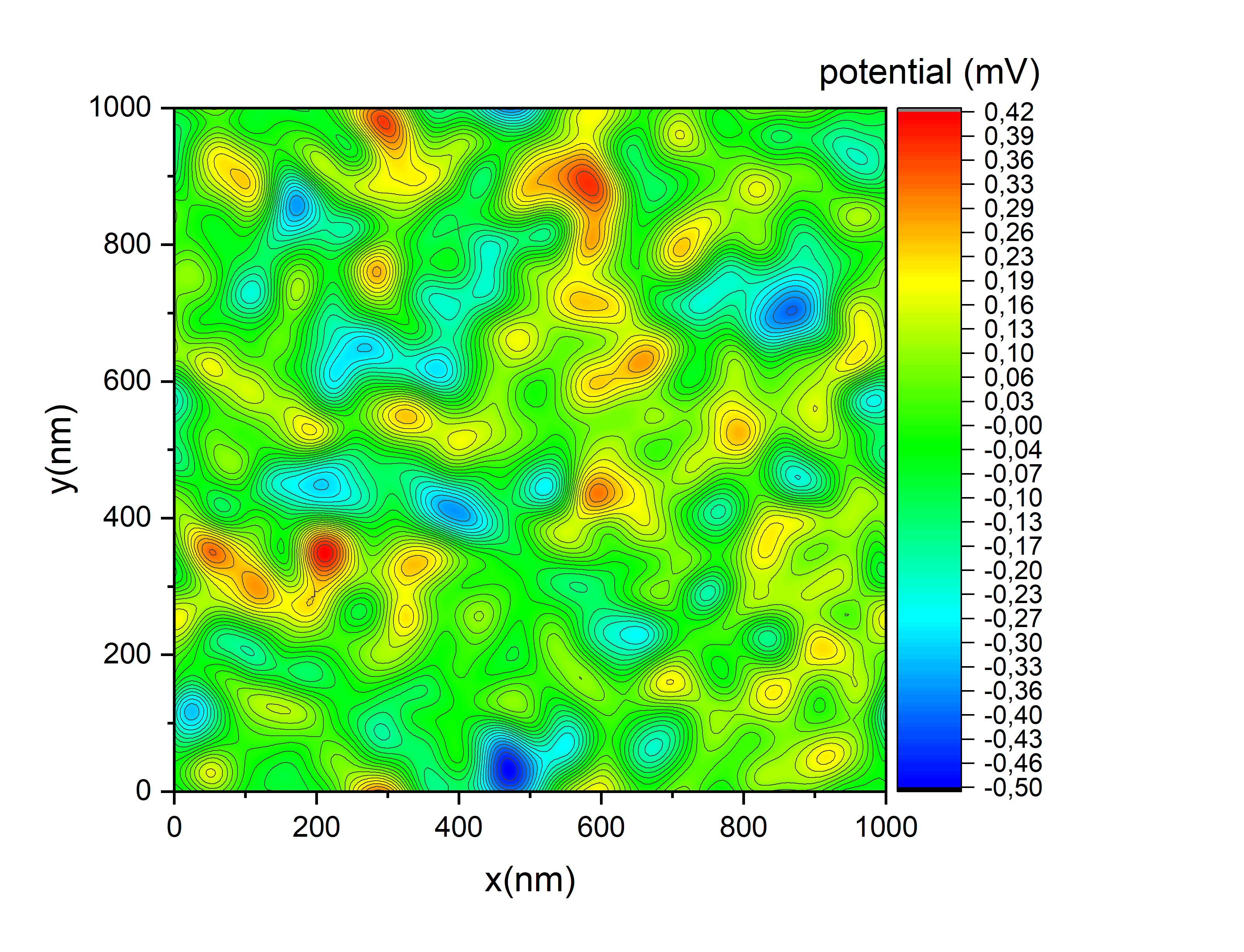
In Fig. S2(a) and (c) one can see that for pure Hartree interaction there is no stripe formation. The density modulation in is much less than in Figs. 1 and S1 and roughly follows the random potential shown in Fig. S3. Furthermore, the charge density modulation in the spin-up and spin-down levels ”repel” each other due to the Hartree interaction. In Fig. S2(b) and (c) we show the situation without interaction. Clearly, there is also no stripe formation. The modulation rather closely follows the random potential of Fig. S3. The charge densities in the spin-up and spin-down levels do not influence each other and follow nearly identically the disorder potential because of any missing interaction.
Hartree non-interacting
(a)  (b)
(b) 
(c)  (d)
(d) 

In order to show that the presence of the remnants of the LL wave functions around each stripe is significant, we perform the calculations of for three test patterns for . The results are given in Fig. S5. We find that only the variation given by as calculated in HF can reproduce essential global features of the experimental NMR results presented in Ref. SFriess2014.


.
In Fig. S6 we show the behavior of for stripes and bubble-like charge density waves. As in Fig. S5, the HF results for lead to a reasonable qualitative agreement with the non-interacting model used in Ref. SFriess2014. Nevertheless, the details around, e.g., are rather different, highlighting the importance of interactions.
– –
(a) (b)
(b)
(c) (d)
(d)
We note that normally stripes appear only starting with filling factor . This is known also experimentally, but for experimental reasons the authors of Ref. SFriess2014 could not go to that filling factor. Instead, they used filling factor and forced, by using an in-plane component of the magnetic field, the electron system to form a stripe pattern. Clearly, there is no need for our simulations to also model this experimental ”trick”. In order to compare the effect of stripe patterns on the NMR Knight shift, we therefore use the stripe pattern in the ”correct” range –. The result in Fig. S6 (b) has striking similarities but seems indeed a bit richer in features than the experimental curve for –. However, since the Knight shift spectrum looses its local information due to the spatial integration, we can also evaluate the range – as shown in Fig. S6. Indeed the agreement with the experiments of Ref. SFriess2014 becomes even better in this filling factor range. We can still see in total 3 peaks, two of them clearly separated and a third one as a shoulder on the high frequency flank, just as shown for the experiments in Fig. 2b of Ref. SFriess2014. This makes the agreement almost perfect for the experiments as shown in Fig. S7 albeit not with the non-interacting modelling of Fig. 2c SFriess2014. Filling factor – requires much more computing time and, although a most interesting question, there are currently no experiments available for comparison.

References
- (1)