The WISSH quasars projectThanks: Based on data obtained with the European Southern Observatory Very Large Telescope, Paranal, Chile, under Program 099.A-0316(A)

We found a Ly$\alpha$-CEN consisting of $\sim$55000 connected voxels by using $SNR_{th}=$2.5 and $N^{vox}_{min}=10000$ pixels. This CEN exhibits a maximum angular extension of $\sim$20 arcsec ($\sim$150 kpc). The line emission integrated over the entire CEN spans a maximum wavelength range of $\sim 95$ Å ($\sim$ 5000 $\rm km\penalty\ s^{-1}$) and shows a peak measured through a Gaussian fit at $\rm\lambda_{Ly\alpha}^{CEN}=(5543.8\pm 1.8)$ Å. This corresponds to a redshift of $\rm z_{CEN}^{Ly\alpha}$ = 3.560$\pm$ 0.002.

Fig. 1 shows the SB map of the Ly$\alpha$-CEN. The nebular emission is the region enclosed in the black thick contour, i.e. the projected boundary derived from the 3D-mask which encloses the detected CEN with $\rm SNR>2.5$. The thin contours indicate the SNR levels derived from the SNR map. This Ly$\alpha$-CEN exhibits a roughly symmetric shape on large scales suggesting a circular (or mildly elliptical) morphology with marked deviations at small radii. In order to obtain a more quantitative description of its morphology we computed the flux weighted centroid shift ($\rm d^{cen}_{CEN}$), the peak displacement ($\rm d^{peak}_{CEN}$), the asymmetry ($\alpha$) and the position angle East of North ($\phi$) of the CEN. The first two quantities were measured with respect to the quasar position, while the remaining ones are estimated from the Stokes parameters as in AB19 (see Table 1). We found general consistency with morphological properties reported by AB19 in the QSO MUSEUM sample. Indeed, both the flux-weighted centroid shift and the asymmetry measured for the Ly$\alpha$-CEN around J1538+08 are close to the median values reported in AB19, i.e. 8.3 kpc and 0.71 respectively. The Ly$\alpha$-CEN exhibits a maximum SB value of $\rm\sim 10^{-16}\penalty\ erg\penalty\ s^{-1}\penalty\ cm^{-2}\penalty\ arcsec^{-2}$ and a total luminosity of $\rm L_{Ly\alpha}=(2.06\pm 0.02)\times 10^{44}$ erg s^-1.

The comparison between the Ly$\alpha$ spectra of the quasar and the CEN normalized to their peak emission is shown in Fig. 2. The quasar spectrum was extracted from an aperture with radius of 3 arcsec, while the CEN spectrum was obtained from the PSF- and continuum- subtracted datacube by summing the spectral contribution of all the spaxels belonging to the CEN (i.e. from the 3D-mask). The x-axis reports the velocity relative to $\rm z_{QSO}$. The white area in the plot corresponds to the spectral width where the CEN was detected (i.e. the maximum spectral extent of the 3D mask; see also Table 1). The red area marks the peak of the Ly$\alpha$ profile of the CEN and includes the errors. The measure of the peak has been obtained through a Gaussian modelling plus a constant continuum term, performed within a range $\pm 500$ Å (or $\pm$ 27,000 $\rm km\penalty\ s^{-1}$) from the Ly$\alpha$ wavelength at $\rm z_{QSO}$. This peak appears to be reasonably (i.e. at $\sim$1$\sigma$) consistent with the $\rm z_{\rm QSO}$ and its 1$\sigma$ uncertainty (yellow area in Fig. 2).

Fig. 3 reports the circularly averaged radial SB profile of the Ly$\alpha$-CEN in J1538+08 (black points) corrected for minimal residual background emission²² 2 Similarly to B16, the SB is estimated at scales much larger than the CEN and the profile is corrected for possible residual background due to unresolved/faint background or foreground (see Appendix A) emission not removed during the continuum subtraction. This subtraction, performed for both the Ly$\alpha$ and the CIV profiles (see Section 4.2), was measured to be negligible accounting for 5-15 $\%$ of the flux of the most external annuli (used for the SB profile) placed at the boundary of each CEN.. The profile was extracted from concentric annular regions centered on the quasar position in the image obtained by collapsing the spectral region in the CEN 3D-mask. The grey area indicates the $2\sigma$ Poisson noise³³ 3 The Poisson noise was estimated as the average value of the standard deviations within background regions $1"\times 1"$ of the pseudo-NB divided by the square root of each annulus area.. The radial profile was compared with the average radial profiles reported by B16 and AB19. All the SB radial profiles in Fig. 3 were corrected for the cosmological $\rm(1+z)^{4}$ SB dimming factor and re-scaled at z=3 for comparison.

We also report the rescaled profile of the CEN around the quasar J0124+00 (which also belongs to the WISSH quasar sample, e.g. Duras et al. 2017), which was identified by B16 as the brightest and most peculiar one in their sample in terms of sharp-peaked morphology, large velocity dispersion and SB radial profile. Both the Ly$\alpha$-CEN around these WISSH quasars exhibit a central (i.e. ¡40-50 kpc) SB excess relative to the B16 and AB19 average profiles.

We further investigated the origin of this SB excess in J1538+08 by comparing the radial profiles extracted for two regions, i.e. south and north of the quasar, which are delimited by the green dashed lines in Fig. 1. Accordingly, the southern region includes the SB peak of the Ly$\alpha$-CEN and the CIV-CEN (see Fig. 4). The SB excess is clearly due to the contribution from the southern region (blue triangles in Fig. 3) at $\leq$20 kpc, while both regions equally contribute to the SB excess at larger radii.

We scanned the datacube searching for diffuse emission in additional ionic transitions typically probing the CGM. The only extended emission detected at good significance level is traced by the CIV line. Given its typically lower emissivity compared with the Ly$\alpha$ we started our search by setting $SNR_{th}=$2.5 and $N^{vox}_{th}=$10000 and then progressively lowered $N^{vox}_{th}$ by steps of 1000 voxels until the extended emission was detected. We found that the $N^{vox}_{th}=4000$ was required to detect this CEN, that indeed consists of 4726 voxels.

The SB map of the CIV-CEN is shown in Fig. 4. The CIV-CEN is much smaller than the Ly$\alpha$-CEN, with a maximum angular extension of $\sim 10$ arcsec, which corresponds to a projected physical size of $\sim$75 kpc. It is almost completely contained in the southern region and exhibits an asymmetric morphology with $\alpha=0.62$. The peak of the $\rm SB_{CIV}$ is located roughly at the same position of the $\rm SB_{Ly\alpha}$ peak, at a distance of $\sim 11.0\pm 3.5\penalty\ \rm kpc$ from the quasar position. The value of the SB peak ($\rm\sim 10^{-17}\penalty\ erg\penalty\ s^{-1}\penalty\ cm^{-2}\penalty\ arcsec^{-2}$) and the luminosity of the CIV-CEN ($\rm L_{CIV}=(9.33\pm 0.33)\times 10^{42}\penalty\ \rm{erg\penalty\ s^{-1}}$) are one order of magnitude lower than those measured for the Ly$\alpha$-CEN.

Fig. 5 shows the comparison between the CIV emission line in the CEN and the quasar spectrum. The CIV-CEN was detected in a relatively narrow spectral range ($\sim 2000\penalty\ \rm{km\penalty\ s^{-1}}$) compared to the spectral region of the Ly$\alpha$-CEN ($\sim 5000\penalty\ \rm{km\penalty\ s^{-1}}$). Through a Gaussian modelling of the line (similarly to the one performed for the Ly$\alpha$), we found that the CIV line peaks at $\rm\lambda_{CIV}^{CEN}=7064.7\pm 1.8$ Å. This corresponds to a redshift of $\rm z_{CEN}^{CIV}$=3.559 $\pm$ 0.001, i.e. in good agreement with the Ly$\alpha$-CEN one. We computed the SB radial profile of the CIV emission (Fig. 6) in the southern region. The emission of the CEN is clearly above the Poisson noise up to $\sim$ 20 kpc from the quasar position.

Figs. 7 and 8 show the flux-weighted velocity maps in regions with SNR$\geq$3 for the Ly$\alpha$- and CIV-CEN, respectively. Each panel reports the velocities relative to the CEN ($\rm z_{CEN}$; left panel) and $z_{\rm QSO}$ (right panel) rest-frame, respectively. There is no significant structure indicative of bulk motion or clear separation between red/blueshifted gas components. Interestingly, almost the entire Ly$\alpha$-CEN exhibits velocities spanning $\sim 1000\penalty\ \rm km\penalty\ s^{-1}$.

We also investigated the radial velocity profile of the Ly$\alpha$-CEN to assess a possible trend with the distance from the quasar. Specifically, we extracted spectra from the PSF- and continuum- subtracted datacube in each annular region used for the SB radial profiles (see Fig. 3). For each spectrum, we modelled the Ly$\alpha$ emission line with a Gaussian profile. Fig. 9 shows the radial distribution of the best-fit velocities relative to the $\rm z_{CEN}$ (blue points). The velocity profile exhibits a constant value around $\sim 100-200\penalty\ \rm km\penalty\ s^{-1}$ up to 15-20 kpc. There is an apparent decline of the velocity down to $-200\penalty\ \rm km\penalty\ s^{-1}$ at larger radii (20-30 kpc).

The flux-weighted velocity dispersion maps for Ly$\alpha$- (left panel) and CIV-CEN (right panel) are shown in Fig. 10. For the Ly$\alpha$-CEN we do not notice any specific gradient as the map shows a nearly constant $\rm\sigma_{v}$ in the range 600-900 $\rm km\penalty\ s^{-1}$ with few regions reaching values larger than 1000$\penalty\ \rm km\penalty\ s^{-1}$. In case of the CIV-CEN the map shows a factor of 2 lower velocity dispersions than the Ly$\alpha$-CEN. Tab. 1 lists the average velocity dispersions ($\bar{\sigma}_{v}$) obtained from these maps. The dispersion estimated through Gaussian model fitting ($\bar{\sigma}_{g}$) of the total spectrum of the Ly$\alpha$- and CIV-CEN is also reported.

In order to better explore the possible presence of a radial gradient of the Ly$\alpha\penalty\$emission velocity dispersion, we computed the radial dispersion profile using the same methodology adopted for the velocity profile (see red points in Fig. 9). The profile exhibits $\sigma_{\rm v}\sim 500\penalty\ \rm km\penalty\ s^{-1}$ up to $\rm\sim 15-20\penalty\ kpc$ and and increase up to $\sigma_{\rm v}\sim 900\penalty\ \rm km\penalty\ s^{-1}$ at $\rm\sim 25\penalty\ kpc$ from the quasar. The profiles could only be accurately computed up to 40 kpc since the line profile modelling at larger distances is completely unconstrained.

We derived a CIV/Ly$\alpha\penalty\$line flux ratio of $0.06\pm 0.01$, in agreement with the approximate values previously estimated for some tentative ($\sim 2.2\sigma-2.8\sigma$) detections of CIV-CEN in B16. Similarly to our result, the B16 values were obtained by estimating the total flux of the voxels associated with the Ly$\alpha$ 3D-Mask shifted at the wavelength of the CIV corresponding to $\rm z_{CEN}$, divided by the total flux of the Ly$\alpha$-CEN (reported in Table 1). This procedure avoids the bias due to aperture effects (i.e. different extensions for different line emissions) and provides a conservative estimate if, as expected, the Ly$\alpha$-CEN is the brightest and more extended one.

The CIV/Ly$\alpha$ ratio map reported in Fig. 11 is the ratio between the CIV and Ly$\alpha$ SB maps over the SNR$\geq$3 regions. The spatial distribution of the ratios suggests that the metal distribution is not completely homogeneous. The median value of the CIV/Ly$\alpha$ ratio directly measured from the CIV/Ly$\alpha$ map is $0.08^{+0.11}_{-0.04}$, where the uncertainties are derived by the 16th and 84th percentiles (corresponding to $\pm$1$\sigma$ for a Gaussian distribution). A consistent value was obtained by computing the SNR-weighted average of the map values of both Ly$\alpha$- and CIV-CEN.

No HeII emission line is visible in the quasar spectrum and no HeII-CEN is detected around J1538+08 at $\rm z_{CEN}$. This is not surprising: while extended HeII emission is commonly observed around high-redshift radio galaxies (e.g. Wilman et al. 2000, Villar-Martín et al. 2007a), it is only found in 6$\%$ of the RQQs in the B16 sample. We inferred a 2$\sigma$ upper limit to the HeII/Ly$\alpha$ ratio of $<0.02$ by applying the same Ly$\alpha$ 3D-mask shift procedure used to obtain the total CIV/Ly$\alpha$ flux ratio.

The integrated profile of the Ly$\alpha$ emission line extracted from the entire CEN and reported in Fig. 2 exhibits a blue tail which can be modelled by an additional component with negative velocity. With the aim of exploring the spatial distribution of this blue tail component, we mapped the asymmetry of the Ly$\alpha\penalty\$emission line profile by using the skewness estimator ($sk$). As for the velocity and dispersion maps, we derived the skewness map as the third moment of the flux distribution according to the following formula:

where $\sum_{i,j,k}^{3D-Mask}$ is the sum on each voxel defined in the 3D-Mask, $\rm F_{i,j,k}$ is the PSF and continuum-subtracted flux from the datacube and $\rm M_{2}$ is the second moment of the flux distribution, defined as:

We found that the southern part of the CEN with skewness values $sk<-0.5$ (blue regions in Fig.12) overlaps with the region of high SB. We verified that other regions do not exhibit skewness at significant levels (i.e. mostly symmetric and low SNR line profiles). The Ly$\alpha$ spectrum extracted from spaxels with $sk\rm<-0.5$ and $\rm SNR\geq 3$ resulted to be clearly asymmetric (Fig. 13). We fit it with two Gaussian components and an additional constant term to account for residual background. The two Gaussian components exhibit significantly different width, with the broad ($\rm\sigma_{v}\simeq 1170\pm$ 260 $\rm\penalty\ km\penalty\ s^{-1}$) component blueshifted by $\rm v_{shift}=1520\penalty\ \pm\penalty\ 360\penalty\ km\penalty\ s^{-1}$ and the narrow one ($\rm\sigma_{v}\simeq 470\pm$ 70 $\rm\penalty\ km\penalty\ s^{-1}$, see Table 2) tracing the systemic $z_{\rm QSO}$. The velocity dispersion found for the narrow component is comparable to the ones reported in Ly$\alpha$-CEN around high-z RQQs (e.g. B16, AB19). The centroid of the narrow component corresponds to a redshift of $z\sim\rm 3.562\pm 0.001$, which is consistent with $\rm z_{QSO}$.

We have reported the discovery of a Ly$\alpha$-CEN around the hyper-luminous RQQ J1538+08, which exhibits a projected size of $\sim$150 kpc and a luminosity of $\rm L_{Ly\alpha}\sim 2\times 10^{44}\penalty\ erg\penalty\ s^{-1}$. Previous MUSE studies at similar redshifts (i.e. $z\sim 3-4$) and exposures (0.75-1 hours) reported Ly$\alpha$-CEN around similarly luminous RQQs (B16) and quasars with slightly lower $\rm L_{bol}$ (AB19). The Ly$\alpha$-CEN around J1538+08 exhibits a maximum projected size which is similar to the average value ($\sim 150$ kpc) found for the B16 sample. The $\rm SB_{Ly\alpha}$ radial profile of our CEN, shown in Fig. 3, exhibits a projected distance from the quasar at a SB of $\rm\sim 10^{-18}erg\penalty\ s^{-1}\penalty\ cm^{-2}\penalty\ arcsec^{-2}$ (i.e. $\sim 50$ kpc), which is similar to the one inferred from the average profiles from B16 and AB19. This behaviour seems to be independent from the luminosity of the quasar (AB19). However, notice that the SB at this distance coincides with the level of the $2\sigma$ Poisson noise of the image and therefore deeper observations are needed in order to verify this claim.

The luminosity of our Ly$\alpha$-CEN is one of the highest measured so far (see Fig. 14) and is comparable to the luminosity of known ELANe (Cantalupo et al. 2014; Hennawi et al. 2015; Cai et al. 2017b; Arrigoni Battaia et al. 2018, e.g,).

Interestingly, some WISSH quasars are included in the B16 (J0124+00, J1621$-$00), AB19 (J0125$-$10, J0947+14) and Cai et al. 2019 (J2123$-$00) samples. The size and luminosity of the Ly$\alpha$-CEN detected around them appear to be heterogeneous (see Fig. 14), suggesting that the properties of these CEN have no simple dependence on the similar, large quasar radiative output (i.e. $\rm L_{bol}$¿$\rm 10^{47}\penalty\ erg\penalty\ s^{-1}$).

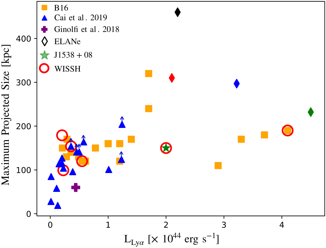
We also checked for possible dependencies on the RQQs bolometric and 2500 Å luminosities (derived from Spectral Energy Distribution modelling; Duras et al. 2017; Duras et al. in prep.) to verify if the nuclear radiative output could affect the properties of the Ly$\alpha$-CEN around the WISSH quasars considered here. However, no significant trend with luminosity was observed, confirming the result reported by AB19 for a larger sample of quasars.

From the velocity maps of the Ly$\alpha$- and CIV-CEN (Figs. 7 and 8) no coherent kinematic structures possibly hinting at bulk motions and rotations were detected. However, the velocity map of the Ly$\alpha$-CEN exhibits a large fraction ($\rm 79_{-10}^{+9}\%$)⁵⁵ 5 Errors derive from the uncertainties to the redshift of both the quasar and nebula. of pixels with SNR$\geq$3 with negative velocities relative to $\rm z_{CEN}$. This can be justified by the presence of the additional blueshifted component in the Ly$\alpha$ line profile (see Sect. 4.5 and Fig. 2). For the CIV-CEN, where we did not detect any significant additional component, the velocity map shows a roughly equal number of pixels with negative and positive velocities. Interestingly, adopting $\rm z_{QSO}$ as reference redshift for the velocity maps of the Ly$\alpha$- and CIV-CEN, we found $\sim$100$\%$ of the SNR$\geq$3 pixels to have negative velocities. Furthermore, our Ly$\alpha$-CEN shows a peak with a negative velocity of - 438 $\pm$ 267$\penalty\ \rm km\penalty\ s^{-1}$. This can be an indication that our $\rm z_{QSO}$ estimated from the H$\beta$ may suffer from systematic uncertainties. Indeed, for a sample of 849 quasars, Shen et al. 2016 found that the determination of the quasar redshift from H$\beta$ is subject to uncertainties as large as $\sim$400 $\rm km\penalty\ s^{-1}$. This can compensate the reported negative velocity offsets of the Ly$\alpha$ peak and the velocity distribution of the SNR$\geq$3 pixels at levels of $\sim$1-2$\sigma$.

Regarding the velocity dispersion, we measured a spatially averaged value $\bar{\sigma_{\rm v}}$= 733 $\pm$ 85 $\rm km\penalty\ s^{-1}$ from the dispersion map (see Table 1). This is a factor of two larger than those measured around the quasars of B16 and AB19 samples, which span the range $\sigma_{\rm v}\approx[200,400]\penalty\ \rm km\penalty\ s^{-1}$. This value is more similar to the reported values for Ly$\alpha$-CEN around high-z radio galaxies in the regions affected by radio jets (van Ojik et al. 1997; Villar-Martín et al. 2003; Humphrey et al. 2006; Silva et al. 2018, $\sigma_{\rm v}\gtrsim 600\penalty\ \rm km\penalty\ s^{-1}$;).

Interestingly, the dispersion map of the Ly$\alpha$-CEN around J1538+08 reports several discrete and compact regions with very high $\sigma_{\rm v}\approx 1000\penalty\ \rm km\penalty\ s^{-1}$ at an average distance from the quasar of 20-30 kpc (see Fig. 10). These high $\rm\sigma_{v}$ regions could be due to the turbulence generated by continuum or line-emitting active sources at $\rm z_{CEN}$, possibly injecting energy into the CGM. However, no continuum sources in the MUSE FOV are associated to high $\rm\sigma_{v}$ values within the Ly$\alpha$-CEN. Similarly to AB19, we used CubExtractor to search for Ly$\alpha$ emitters by setting $\rm SNR_{th}>5$ and $N_{min}^{vox}=50$. We did not detect any source within the CEN. We only found a source with a flux of $\rm 3.5\times 10^{-16}\penalty\ erg\penalty\ s^{-1}\penalty\ cm^{-2}$, at the redshift of the CEN (z$\approx$3.560), outside its boundaries and at a projected distance of $\sim$250 kpc from the quasar (RA = 15:38:28.7, Dec = +8:55:00.80), which very likely cannot affect the nebular emission.

The CIV-CEN revealed around J1538+08 is one of the few extended (75 kpc) CIV-emitting regions detected at high significance ($5\sigma$)⁶⁶ 6 This value represents the integrated SNR computed for the extended CIV emission line. and spatially mapped around a RQQ. This provides a clear indication of a metal enriched medium (i.e. non-pristine) around this quasar. The luminosity of this CEN ($\rm L_{CIV}\simeq 10^{43}\rm erg\penalty\ s^{-1}$) is comparable to those measured for CIV-CEN detected around radio galaxies at similar redshift (Villar-Martín et al. 2007a). However, its morphology shows a marked asymmetry relative to the central quasar position. This is at odds with symmetrically distributed CEN reported around radio galaxies (Villar-Martín et al. 2007b; Silva et al. 2018, e.g.). Interestingly the ratio between the SB radial profiles of the CIV and Ly$\alpha$ reported in Fig. 6 (i.e. in the southern wedge containing the SB Ly$\alpha$ peak and the CIV-CEN) is a factor of $\sim$0.1 and is constant up to $\rm\sim 25$ kpc (i.e. the distance where the Poisson noise starts to dominate the CIV-CEN radial profile). This evidence and the spatial co-location of the SB peaks of the two CEN suggest that they could be tracing the same gas and, hence, triggered by the same mechanism. Deeper observations would hopefully reveal fainter CIV emission with the same size and morphology of the Ly$\alpha$-CEN in J1538+08.

The possible powering mechanisms of the Ly$\alpha$-CEN include quasar photoionization (i.e. fluorescence), collisional excitation (i.e. cooling) and shocks. In case of fluorescence, assuming that the quasar is surrounded by cold and spherical clouds, we can estimate the CEN SB in two extreme regimes: optically thin (with column density $\rm N_{H}\ll 10^{17.2}cm^{-2}$) and optically thick (Hennawi & Prochaska 2013, $\rm N_{H}\gg 10^{17.2}cm^{-2}$;). We obtain $\rm SB_{Ly\alpha}^{thick}\simeq 2.8\times 10^{-15}\penalty\ erg\penalty\ s\penalty\ cm^{-2}\penalty\ arcsec^{-2}$ and $\rm SB_{Ly\alpha}^{thin}\simeq 2.2\times 10^{-18}\penalty\ erg\penalty\ s\penalty\ cm^{-2}\penalty\ arcsec^{-2}$, for optically thick⁷⁷ 7 The luminosity at the Lyman edge, required by the formula (15) by Hennawi & Prochaska 2013, has been estimated by the $\rm L_{1450}$ (see Duras et al. in prep.) as detailed in Lusso et al. 2015 and Farina et al. 2019. Moreover, we adopted as CEN radius 40 kpc (see Fig. 3) and a covering factor $\rm f_{c}=0.5$ and optically thin⁸⁸ 8 We used the formula (10) in Hennawi & Prochaska 2013 and adopted the following fiducial values: $\rm N_{H}=10^{20}\penalty\ cm^{-2}$, density $\rm n_{H}=0.1\penalty\ cm^{-3}$ and $\rm f_{c}=0.5$. gas, respectively. In our case, we found that $\rm SB_{Ly\alpha}$ for regions with SNR$\geq$3 is $\rm\simeq 2.3\times 10^{-17}\penalty\ erg\penalty\ s\penalty\ cm^{-2}\penalty\ arcsec^{-2}$. This value is more compatible to $\rm SB_{Ly\alpha}^{thin}$ than to $\rm SB_{Ly\alpha}^{thick}$, supporting the presence of an optically thin medium as already reported in previous works (e.g. AB19, Cai et al. 2019).

The CIV/Ly$\alpha$ and HeII/Ly$\alpha$ ratios could be used to understand if shocks or collisional excitation are viable powering mechanisms for the observed Ly$\alpha$-CEN (Cantalupo et al. 2019, but see). The detection of the CIV-CEN allows us to rule out cooling due to gravitational accretion as the powering mechanism of this CEN. However, it is notoriously difficult to disentangle photoionization models from shock models in a HeII/Ly$\alpha$ vs CIV/Ly$\alpha$ diagram (Arrigoni Battaia et al. 2015a). Nevertheless, photoionization models usually do not predict lower levels of HeII/Ly$\alpha$ with respect to CIV/Ly$\alpha$ (Humphrey 2019; Cantalupo et al. 2019, e.g.,). On the contrary they predict ratios of the same order for the two transitions. This is because these two emission lines have similar ionization energies 64.5 eV for CIV and 54.4 eV (4 Ryd) for HeII. On the other hand, shock models (Allen et al. 2008) do show cases in which the HeII/Ly$\alpha$ ratio is lower than the CIV/Ly$\alpha$ ratio. Indeed, according to shock+precursors models presented by Allen et al. 2008 and Arrigoni Battaia et al. 2015b for the origin of extended nebular emission, the values of CIV/Ly$\alpha$ and HeII/Ly$\alpha$ inferred from our analysis are consistent with a shock propagating at 200-300 $\rm km\penalty\ s^{-1}$ in a $\rm n_{H}\sim 10-100\penalty\ cm^{-3}$ gas or with a faster ¿1000 $\rm km\penalty\ s^{-1}$ shock in a denser gas ($\rm n_{H}>100\penalty\ cm^{-3}$). If we assume that the $\rm v_{shift}=1520\penalty\ km\penalty\ s^{-1}$ is the velocity of the shock, then the emitting gas is required to be at high densities ($\rm n_{H}>100\penalty\ cm^{-3}$).

The aforementioned photoionization and shock models do not include a contribution from resonant scattering of Ly$\alpha$ photons from the quasar. In the case such contribution is important, the CIV/Ly$\alpha$ and HeII/Ly$\alpha$ ratios predicted by those models needs to be corrected and shifted to lower values. However, it has been shown that the efficient diffusion in velocity space allows the Ly$\alpha$ resonantly scattered photons produced by the quasar itself to escape the system at very small scales, $<10$ kpc (Dijkstra et al. 2006). Therefore, this should result in a negligible contribution of scattered Ly$\alpha$ emission on scales $>10$ kpc (Cantalupo et al. 2014, e.g,). A firm characterization of the Ly$\alpha$ resonant scattering contribution requires a full radiative transfer calculation on a three dimensional gas distribution representing this system. This approach is beyond the scope of this work.

The blueshifted broad component in the Ly$\alpha$ spectrum of the CEN provides a tantalizing evidence for the presence of outflowing gas reaching a projected distance of 20-30 kpc from the quasar, i.e. into the CGM surrounding J1538+08.

J1538+08 also exhibits a host-galaxy scale [OIII] outflow with mass outflow rate $\rm\sim 530\penalty\ M_{\odot}\penalty\ yr^{-1}$, maximum velocity $\rm\sim 2900\penalty\ km\penalty\ s^{-1}$ and kinetic power of $\rm\dot{E}_{kin}=1.4\times 10^{45}\penalty\ erg\penalty\ s^{-1}$ (Vietri et al. 2018, see). In an energy conserving scenario in which the large-scale outflow reported in this paper is the later stage of the AGN-driven [OIII] one (Bischetti et al. 2017; Vietri et al. 2018, e.g.), by assuming an expansion at $\rm v_{out}=v_{shift}\sim 1500\penalty\ km\penalty\ s^{-1}$, we estimated a mass outflow rate of $\rm\dot{M}_{out}\simeq 300\penalty\ M_{\odot}\penalty\ yr^{-1}$, comparable to the [OIII] one. Notice that, assuming $\rm v_{out}=300\penalty\ km\penalty\ s^{-1}$ as suggested by the CIV/Ly$\alpha$ and HeII/Ly$\alpha$ values in a shock+precursor models (see Sect. 5.3) we would obtain a $\rm\dot{M}_{out}$ larger by a factor of 25, but still comparable with the typical $\rm\dot{M}_{out}$ reported for [OIII] outflows in the WISSH sample (Bischetti et al. 2017). By assuming a constant velocity of 1500$\rm\penalty\ km\penalty\ s^{-1}$ (see Tab. 2), we estimated that an outflow at host galaxy scales (Bischetti et al. 2017, i.e. $\sim$5-10 kpc ) would take $\sim$7-13 Myr to reach the distance of our CGM outflow (i.e. $\sim$30 kpc). Adopting a velocity of $\sim$300$\rm\penalty\ km\penalty\ s^{-1}$, we would obtain an upper limit to the outflow time a factor of 5 larger than the previous estimate.

The sudden increase of the velocity dispersion of the Ly$\alpha$-CEN to $\sigma_{\rm v}\sim$900$\rm\penalty\ km\penalty\ s^{-1}$ at a distance of $\sim$20 kpc (see Fig. 9) could be partially due to the presence of the outflow component, hence to an incorrect parameterization of the line profile with a single Gaussian component. Unfortunately the SNR of our observations does not allow us to recompute the radial profile of the $v$ and $\sigma_{\rm v}$ of the Ly$\alpha$ line using a two-component Gaussian modelling, because the SNR of the broad Ly$\alpha$ line in each bin is too low. Deeper MUSE observations are therefore needed to verify the presence of a broad and blueshifted component over the entire Ly$\alpha$-CEN and assess if the CIV-CEN also shares the same kinematics.

Given the resonant nature of the Ly$\alpha$ transition, complex radiative transfer models accounting for the velocity field, density structure of the CEN and the geometry of the radiation field are needed in order to properly interpret the properties derived by the Ly$\alpha$ line profile fitting (Cantalupo et al. 2005; Gronke & Dijkstra 2016, e.g.). It is worth noting that the presence of an expanding shell surrounding the quasar, assuming spherical symmetry and isotropic geometry of the photoionizing radiation field, may produce an asymmetric double peak profile in which the blue-ward component is strongly suppressed (Verhamme et al. 2006; Laursen et al. 2009; Steidel et al. 2010; Chung et al. 2019). This would provide support to the hypothesis of an outflowing CEN whose two components of the Ly$\alpha$ profile are associated with the same expanding gas. Notice that in this simple model (i.e. symmetric, homogeneous and isotropic gas distribution) the main peak component is always on the red side compared with the systemic redshift of the CEN. However, assuming that $z_{\rm QSO}\equiv z_{\rm CEN}$, our Ly$\alpha$-CEN does not show such a red line component (see Fig.13). To test the nature of this putative outflow in the context of an asymmetric, inhomogeneous gas distribution, MUSE observations with higher SNR are needed along with a more accurate determination of $z_{\rm QSO}$ (e.g. from the CO line) and radiative transfer models.