When $\tan\beta$ meets all the mixing angles

A preferred basis is only singled out by first imposing a certain symmetry (gauge, global, or discrete). The general scalar potential then reduces to a particular form. In particular, when using the reflection symmetry $\mathbb{Z}_{2}$, the non-physical parameter $\tan\beta$ can then be defined with respect to this basis and thereby promoted to a physical parameter. Additionally, if symmetry-breaking effects are allowed, the identification of this parameter as physical gets more subtle. For a thorough discussion on the physical meaning of $\tan\beta$, see Ref. Haber and O’Neil 2006.

In 2HDMs with $\mathbb{Z}_{2}$, there is natural flavour conservation Paschos 1977; Glashow and Weinberg 1977, that is, absence of flavour-changing-neutral-currents (FCNCs) at tree- and loop-level. Interestingly, the Yukawa interactions get parametrised by the corresponding Yukawa couplings and $\tan\beta$. One could thus naturally wonder if fermion mixing has anything to do with this parameter. This possibility was realized only recently Das 2019. There it was found that by enlarging the discrete symmetry $\mathbb{Z}_{2}$ to $\mathbb{D}_{4}\simeq\mathbb{Z}_{4}\rtimes\mathbb{Z}_{2}$ and by a judicious assignment of the quarks and the two scalars to irreducible representations of $\mathbb{D}_{4}$ Ishimori et al. 2010, then the Cabibbo angle, $\theta_{c}\simeq 0.22$, can be directly related to $\beta$ as:

The proposal in Das 2019 is a first attempt where the first generation of quarks remains massless and there is no allowed mixing with the third quark generation. It is our goal here to offer a complete framework where all quarks are massive and their mixings are consistent with the most up-to-date global fits, and similarly for the leptons.

There has already been various efforts towards the construction of a successful $\mathbb{D}_{4}$ flavor model Grimus and Lavoura 2003; Grimus et al. 2004; Blum et al. 2008; Adulpravitchai et al. 2009; Hagedorn and Ziegler 2010; Meloni et al. 2011. For example, from a rather general point of view Ref. Blum et al. 2008 offers a thorough discussion of the major implications of using dihedral groups. Unfortunately, none of them explored the possibility of relating the masses and mixing parameters to $\tan\beta$. Our purpose here is to explore this relation as a direct consequence of $\mathbb{D}_{4}$. Therefore, we will not consider further auxiliary symmetries that could reduce the number of free parameters.

This letter is organized as follows. In Sec. II we describe the model. In Sec. III we discuss the scalar potential and show how to produce hierarchical VEVs. In Secs. IV and V we show how the mixing angles can be related to $\tan\beta$. We discuss the main features and phenomenological consequences of the model in Secs. VI, VII, VIII, and IX. Finally, our conclusions are stated in Sec. X. To keep the discussion short we have delegated all technical details to Appendices.

In contrast to Ref. Das 2019, we use a different basis Ishimori et al. 2010; Meloni et al. 2011 for the generators of the two-dimensional representations¹¹ 1 This choice directly impacts the tensorial products, as shown in Eq. (62).

where ${\bf a}$ and ${\bf b}$ denote the generators of $\pi/2$ rotations and reflections, and are order four and two, respectively: ${\bf a}^{4}={\bf 1}_{2\times 2}={\bf b}^{2}$. Notice that our generators are complex. Since the representations are real, there is a unitary matrix ${\bf\sigma}_{1}$ that connects the generators to the complex conjugates:

As a consequence, for any given flavor doublet, ${\bf g}=(g_{1},g_{2})^{T}$, when considering the conjugate, it is the combination $\sigma_{1}{\bf g}^{*}$ that transforms as a doublet, not simply ${\bf g}^{*}$. Furthermore, realize the main advantage of choosing the aforementioned complex generators: the up and down components of the flavor doublet have definite $\mathbb{Z}_{4}$ charge which could later turn to be useful if breaking the flavor symmetry into a particular subgroup. For further details see Ref. Ishimori et al. 2010.

We make the following representation assignments in the quark sector (we use the subindex “$D$” to denote the $\mathbb{D}_{4}$ doublets):

whereas in the lepton sector we assign:

Here we use the notation of Ref. Ishimori et al. 2010 for the one-dimensional representations, namely $1_{b,ab}$ ($i.e.$ the signs indicate the transformation of the field under $b$ and $ab$, respectively).

Our choice allows a later reinterpretation of the model as having the appearance of a 2HDM with softly-broken natural flavour conservation. Notice that we are also considering $\mathbb{D}_{4}$-assignments of the leptonic fields, which are not included in the work of Ref. Das 2019, as is only focused on the description of the quark sector.

On the other hand, the scalar sector, which is composed of three Higgs doublets, has the assignments

There are other possibilities $\Phi_{S}\sim\{{\bf 1}_{++},{\bf 1}_{--},{\bf 1}_{+-}\}$ (for more details see Appendix D), however, not all of the resulting mass matrices give the correct masses and mixings. Note that the scalar doublet $\Phi_{S}$ is a necessary element as by virtue of it we introduce mixing with the third generation and a non-zero mass for the first fermion family. Moreover, as seen later, it can also be used to give mass to the bottom quark and tau lepton, opening the parameter space to more viable solutions. In what follows, we also use $\widetilde{\Phi}=i\tau_{2}\Phi^{\ast}$, where $\tau_{2}$ is the Pauli matrix in $SU(2)_{L}$ space.

The Yukawa Lagrangian for the quark sector is ${\cal L}_{Y}^{Q}={\cal L}_{Y}^{(u)}+{\cal L}_{Y}^{(d)}$, where

whereas for the lepton sector is ${\cal L}_{Y}^{\ell}={\cal L}_{Y}^{(e)}+{\cal L}_{Y}^{(\nu)}$, with

Note that we have three complex parameters for the up quark mass matrix, and also three for the Dirac neutrino mass matrix, while we have four complex parameters for the down quark and the charged lepton mass matrices; and finally, two real parameters for the mass matrix of the Majorana neutrinos, $N_{1R}$ and $N_{2R}$. Now, a phase field redefinition can make all the phases in the up quark mass matrix to be zero while only two and three in the down quarks and charged leptons, respectively, as obtained in Appendix B. Therefore, we choose to keep as complex parameters, in the down quark and charged lepton mass matrix, only $\{y_{3}^{d},y_{4}^{d}\}$ and $y_{4}^{e}$. Thus we are left with 7 real magnitudes and 2 relevant complex phases in the quark sector, while 9 real magnitudes and 4 complex phases in the lepton sector (including the two Majorana masses). The 9 (13) arbitrary parameters in the quark (lepton) sector must describe 10 (12) mass and mixing parameters. Hence, it is only in the quark sector that we expect the strongest correlations.

We assume $\mu_{D}^{2}<0$ while $\mu_{S}^{2}>0$, such that

As long as the flavour symmetry is not broken, the minimum conditions:

enforce two independent solutions: the symmetric limit, $v_{1}=v_{2}$, or one in which one of the two VEVs is zero while the other is equal to $\sqrt{-\mu_{D}^{2}/(\lambda_{4}+\lambda_{5})}$.

In the following, we choose the latter possibility. Now, if we wish to explore the case where the null VEV in the flavour doublet is no longer zero but still rather small, i.e. $v_{2}\sim{\cal O}(10^{-2}-10^{-1})\,v_{1}$, we need to softly-break the symmetry by introducing

where to conserve CP we assume $\mu_{12}^{2}$ to be real and we require $\mu_{12}^{2}\ll\mu_{D}^{2}$ and also $\mu_{12}^{2}>0$. Furthermore, it is also necessary to break the mass scale between $\Phi_{1}$ and $\Phi_{2}$. For this purpose, we add $\mu_{2}^{2}\Phi_{2}^{\dagger}\Phi_{2}$.

Realize that as we are also interested in inducing a VEV in the flavour singlet isodoublet, $\Phi_{S}$, we need to add an extra soft-breaking term. Now, to make its VEV smaller than $v_{2}$ we choose $\Phi_{2}$ and not $\Phi_{1}$ as the one responsible for inducing it. The complete $non-symmetrical$ expression therefore reads

This choice allows us to write the following relations

If we consider $\lambda_{k}\sim{\cal O}(1)$, and $|\mu_{D}|\sim{\cal O}(100)\text{ GeV}$, $\mu_{2}\sim{\cal O}(100)\text{ GeV}$, $\mu_{12}\sim{\cal O}(10)\text{ GeV}$, $\mu_{S2}\sim{\cal O}(0.1-1)\text{ TeV}$, and $\mu_{S}\sim{\cal O}(1)\text{ TeV}$ then we expect $v_{1}\sim{\cal O}(100)\text{ GeV}$, $v_{2}\sim{\cal O}(10)\text{ GeV}$, and $v_{s}\sim{\cal O}(1)\text{ GeV}$. In other words, $v_{2}=\epsilon v_{1}$ and $v_{s}=\epsilon^{2}v_{1}$ with $\epsilon\sim 10^{-1}$. Now, note that this hierarchy in the VEVs allows us to say that to a very good degree of approximation

and we are still able to write

With this definition we can reexpress the small VEVs in the following way

where we have already considered $v_{1}\simeq v$ and

To illustrate the order of the scalar masses we consider a simple benchmark scenario where $\lambda_{2,3,6,7,8}=0$, $\lambda_{4}=\lambda_{5}$, and $\lambda_{1,4,5}\sim{\cal O}(1)$. This scenario has the great advantage of simplifying Eq. (14) to

and allowing a qualitative analysis of both the scalar masses and the hierarchical VEVs in terms of the same set of parameters $\{\mu_{D}^{2},\mu_{2}^{2},\mu_{12}^{2},\mu_{S}^{2},\mu_{S2}^{2},\lambda_{1},\lambda_{5}\}$. The complete and exact mass matrices are shown in Appendix C. The scalar mass matrices, for this case, then read

where we have neglected small contributions when appropriate. The CP-odd and charged scalar mass matrices are consistent with only one massless state. Furthermore, in this benchmark scenario, the physical CP odd neutral and electrically charged scalars are exactly degenerate, which is an scenario favoured by electroweak precision tests Cárcamo Hernández et al. 2015. It is then straightforward to obtain that the lightest scalar state of mass $125\text{ GeV}$ while all the heavy states (neutral and charged) have masses in agreement with all the current experimental constraints. In fact, we have performed a numerical analysis of the scalar sector obtaining a large number of solutions for the scalar masses consistent with experimental bounds. In our analysis we have required that the mass for the lightest CP even neutral scalar state to be in the $3\sigma$ experimentally allowed range $124.96$ GeV$\leqslant m_{h}\leqslant$ $125.8$ GeV Sirunyan et al. 2020, whereas for the heavy CP even neutral scalar masses we require them to be larger than $200$ GeV, as done in Hernandez-Sanchez et al. 2020. The masses for the physical CP odd and electrically charged scalars are required to be larger than their lower experimental bounds of $93.4$ GeV and $90$ GeV, respectively Tanabashi et al. 2018. We have found that the heavy scalar masses feature linear correlations as shown in Figure 1.

We calculate the unitary transformations diagonalizing the mass matrices from the hermitian mass matrix product, ${\bf H}={\bf M}{\bf M}^{\dagger}$,

If we were to try to fit the quark masses and mixing with those contributions that remain when setting $y_{4}^{d}$ to zero, we would find out that it is not possible. In fact, in all those settings appearing in Appendix D with $y_{4}^{d}=0$ there is no viable phenomenology. The natural advantage of considering its contributions is that thanks to the amount of suppression in $v_{s}\sim\beta^{2}v_{1}$, we can make them responsible for introducing the mass of the bottom quark with $y_{4}^{d}\sim{\cal O}(1)$ together with the right mixing, as shown in Appendix E. This observation is what allows the present framework to be viable.

Notice that when $v_{s}\rightarrow 0$, the up- and down-type quark mass matrices shown in Eq. (23) are diagonalised by the orthogonal transformation

Hence, the leading contribution to quark mixing is obtained from

from which one easily sees that Eq. (1) is satisfied up to a sign

In fact, we would have obtained a positive sign if the right-handed fermions of the third family had initially exchanged their assignments, i.e.

Nevertheless, within the original relation ($\theta_{c}=+2\beta$), it is not possible to find a good agreement of the mixing parameters with their experimental value. Therefore, we conclude from here that in a complete $\mathbb{D}_{4}$-framework with three Higgs doublets and where all quark mixing phenomena is explained, the correct relation between the Cabibbo and $\beta$ angle requires a minus sign, as in Eq. (26). In Appendix E, we give all the necessary details to understand the aforementioned observation and also realize how the mixing angles get expressed in terms of $\beta$.

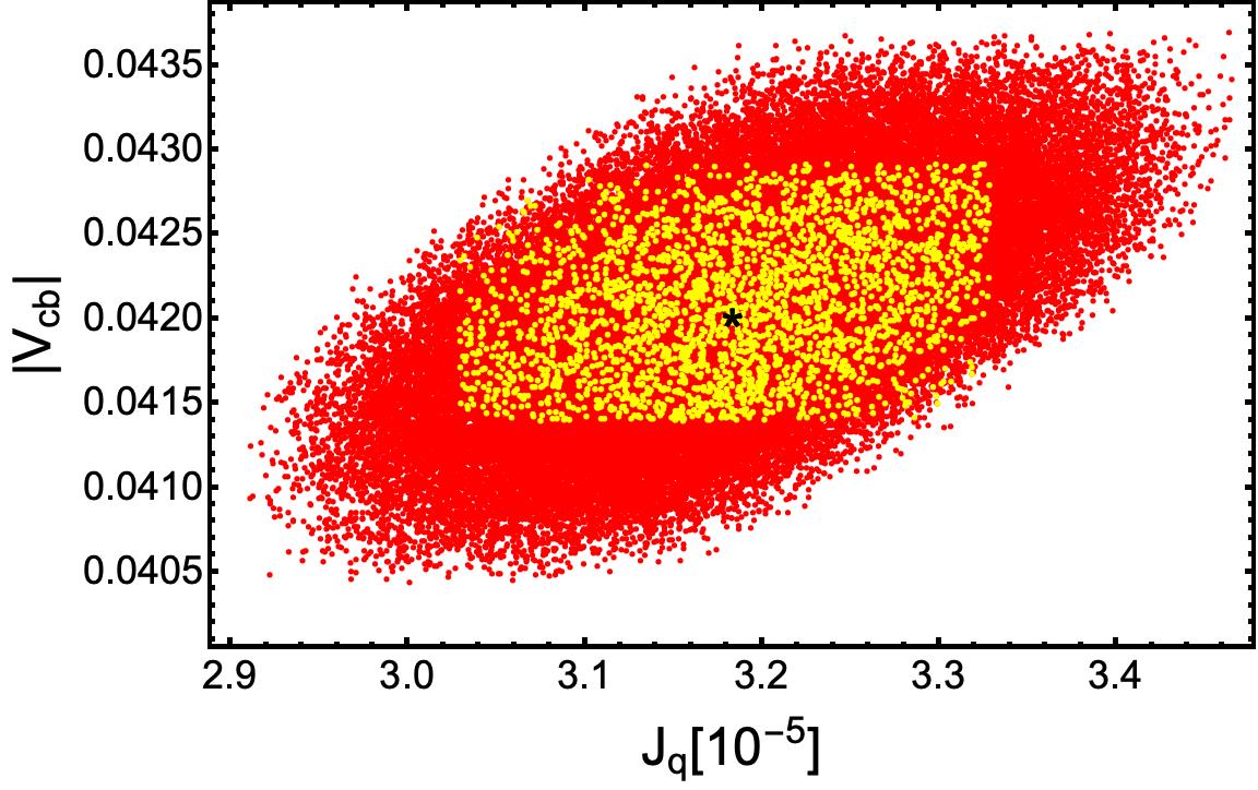
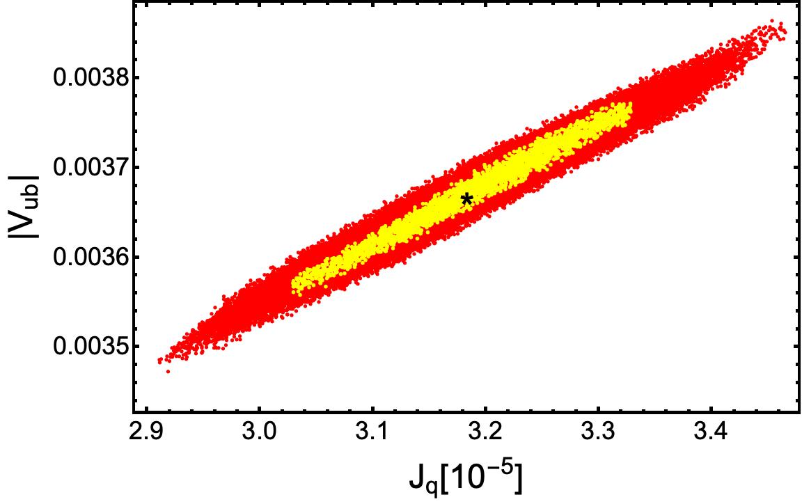
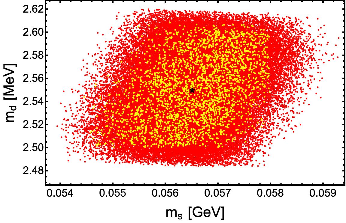
We have performed a numerical analysis of the quark mass matrices and found a wide region of parameter space where the obtained values of the quark mixing angles, Jarlskog invariant and the up and down type quark masses are consistent with the experimental data, see Appendix F.

The following best-fit values,

reproduce all the quark masses and the observed quark mixing at the $1\sigma$ level with a quality of fit of $\chi^{2}_{\text{d.o.f.}}=0.10$. The correlations of the quark mixing angles with the Jarlskog invariant are shown in Figure 2. Interestingly, while doing the fit we find that the relation $|\theta_{c}|=2|\beta|$ receives significant contributions. Therefore, instead of using the value $|\beta|\simeq|\theta_{c}|/2$ we explicitly employed $|\beta|=0.047$. Further details have been delegated to Appendix F.

Assuming that the right-handed Majorana neutrinos have masses much larger than the electroweak symmetry breaking scale, $\{M_{1},M_{2}\}\gg v_{1}$, one has that the light active neutrino masses are generated from a type I seesaw mechanism that gives rise to an effective Majorana mass matrix

The lepton mass matrices show some interesting features. In the limit $\beta\rightarrow 0$, the solar, reactor, and atmospheric mixing angles go to zero as well as the first family of lepton masses. This can be obtained from noting that, in the limit $\beta\rightarrow 0$, Eqs. (29) and (30) take the form

thus implying that the effective Majorana mass matrix for neutrinos turns into

favouring the inverted ordering case. However, in general, for $\beta\neq 0$ the hierarchical structure among the mass matrix elements strongly depends upong the heavy Majorana masses. This means that depending on $M_{1}\gg M_{2}$ or $M_{1}\ll M_{2}$ the model could either favour the normal ordering case, $m_{\nu 3}>m_{\nu 2}>m_{\nu 1}$, or the inverted one, $m_{\nu 2}>m_{\nu 3}>m_{\nu 1}$, respectively.

We have performed a numerical analysis and found that in order to successfully accommodate the experimental values of the leptonic mixing angles, the leptonic CP violating phase and the neutrino mass squared splittings, soft-breaking Majorana terms need to be introduced. The correlations of the effective mass parameter of neutrinoless double beta decay with the lightest neutrino mass and leptonic CP phase for the scenario of normal neutrino mass hierarchy are shown in Figure 3.

In the quark sector, the Yukawa matrices parametrising the coupling to each Higgs doublet $\{\Phi_{1},\Phi_{2},\Phi_{S}\}$ are denoted by ${\bf\Gamma}_{1},{\bf\Gamma}_{2},{\bf\Gamma}_{S}$, respectively. In the fermionic mass basis, they take the explicit form,

where we have also employed $v_{1}\simeq 174\text{ GeV}$, $v_{2}\simeq 8.14\text{ GeV}$, and $v_{s}\simeq 2.63\text{ GeV}$.

Now, in the scalar sector, we consider an explicit realization of the previously discussed benchmark scenario. There we assume

and through Eq. (14), $v_{2}\simeq 8.14\text{ GeV}$, and $v_{s}\simeq 2.63\text{ GeV}$ we obtain the explicit value for $\{\mu_{2},\mu_{S2}\}$. This explicitly imply a degenerate scalar mass spectra:

It is interesting to also remark here an important feature of our model: although we have small VEVs the scalar masses are very heavy. This is due to the fact on how we softly-broke the flavour symmetry and went into inducing VEVs.

The orthogonal transformation bringing the scalar sector to its mass basis is approximately characterized by the same matrix

where we follow the convention ${\bf R}{\bf m}^{2}{\bf R}^{T}={\bf m}^{2}_{\text{diag}}$. Notice how the smallness of the off-diagonal elements in ${\bf R}$ imply additional suppression factors when computing FCNCs. That together with the fact that all the scalars, neutral and charged, have sufficiently heavy masses guarantee that FCNCs should be well below their upper bounds.

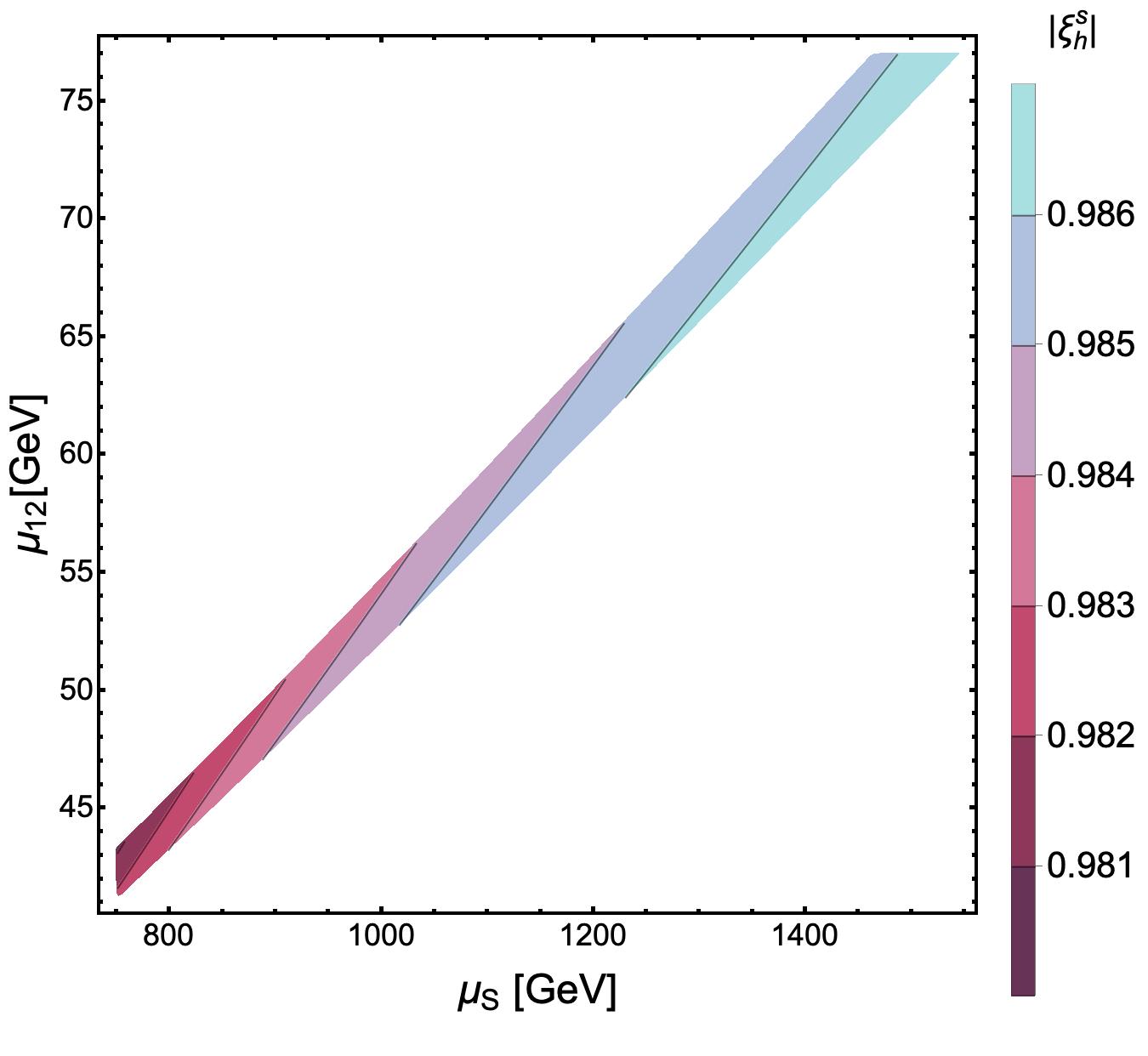
On the other hand, we can now also investigate the effective couplings between the fermions and the SM-like Higgs:

where

In our case, we find for $\mu_{12}\in[35,77]\text{ GeV}$ and $\mu_{S}\in[750,2000]\text{ GeV}$ the ranges:

which are in agreement to the most recent combined fits of data taken at $\sqrt{s}=13\text{ TeV}$ Sirunyan et al. 2019

while the lightest families to the latest global fits Kagan et al. 2015; Perez et al. 2015 with large upper bounds $\kappa_{f}<{\cal O}(10-100)$. Note how Figure 4 shows a correlated behaviour between the strange and bottom quarks: the larger the one the smaller the other, for a discussion on the reach on projected sensitivities of future colliders see de Blas et al. 2020. We expect the analysis for the charged-leptons to be very similar to the down quarks, as they have similar fermion mass spectra and a similar structured mass matrix.

References

- Lee (1973) T. D. Lee, Phys. Rev. D8, 1226 (1973), [,516(1973)].
- Branco et al. (2012) G. C. Branco, P. M. Ferreira, L. Lavoura, M. N. Rebelo, M. Sher, and J. P. Silva, Phys. Rept. 516, 1 (2012), arXiv:1106.0034 [hep-ph] .
- Haber and O’Neil (2006) H. E. Haber and D. O’Neil, Phys. Rev. D74, 015018 (2006), [Erratum: Phys. Rev.D74,no.5,059905(2006)], arXiv:hep-ph/0602242 [hep-ph] .
- Paschos (1977) E. A. Paschos, Phys. Rev. D15, 1966 (1977).
- Glashow and Weinberg (1977) S. L. Glashow and S. Weinberg, Phys. Rev. D15, 1958 (1977).
- Das (2019) D. Das, Phys. Rev. D100, 075004 (2019), arXiv:1908.03961 [hep-ph] .
- Ishimori et al. (2010) H. Ishimori, T. Kobayashi, H. Ohki, Y. Shimizu, H. Okada, and M. Tanimoto, Prog. Theor. Phys. Suppl. 183, 1 (2010), arXiv:1003.3552 [hep-th] .
- Grimus and Lavoura (2003) W. Grimus and L. Lavoura, Phys. Lett. B 572, 189 (2003), arXiv:hep-ph/0305046 .
- Grimus et al. (2004) W. Grimus, A. S. Joshipura, S. Kaneko, L. Lavoura, and M. Tanimoto, JHEP 07, 078 (2004), arXiv:hep-ph/0407112 .
- Blum et al. (2008) A. Blum, C. Hagedorn, and M. Lindner, Phys. Rev. D 77, 076004 (2008), arXiv:0709.3450 [hep-ph] .
- Adulpravitchai et al. (2009) A. Adulpravitchai, A. Blum, and C. Hagedorn, JHEP 03, 046 (2009), arXiv:0812.3799 [hep-ph] .
- Hagedorn and Ziegler (2010) C. Hagedorn and R. Ziegler, Phys. Rev. D 82, 053011 (2010), arXiv:1007.1888 [hep-ph] .
- Meloni et al. (2011) D. Meloni, S. Morisi, and E. Peinado, Phys. Lett. B 703, 281 (2011), arXiv:1104.0178 [hep-ph] .
- Cárcamo Hernández et al. (2015) A. E. Cárcamo Hernández, S. Kovalenko, and I. Schmidt, Phys. Rev. D91, 095014 (2015), arXiv:1503.03026 [hep-ph] .
- Sirunyan et al. (2020) A. M. Sirunyan et al. (CMS), (2020), arXiv:2002.06398 [hep-ex] .
- Hernandez-Sanchez et al. (2020) J. Hernandez-Sanchez, C. G. Honorato, S. Moretti, and S. Rosado-Navarro, (2020), arXiv:2003.06263 [hep-ph] .
- Tanabashi et al. (2018) M. Tanabashi et al. (Particle Data Group), Phys. Rev. D98, 030001 (2018).
- Sirunyan et al. (2019) A. M. Sirunyan et al. (CMS), Eur. Phys. J. C 79, 421 (2019), arXiv:1809.10733 [hep-ex] .
- Kagan et al. (2015) A. L. Kagan, G. Perez, F. Petriello, Y. Soreq, S. Stoynev, and J. Zupan, Phys. Rev. Lett. 114, 101802 (2015), arXiv:1406.1722 [hep-ph] .
- Perez et al. (2015) G. Perez, Y. Soreq, E. Stamou, and K. Tobioka, Phys. Rev. D 92, 033016 (2015), arXiv:1503.00290 [hep-ph] .
- de Blas et al. (2020) J. de Blas et al., JHEP 01, 139 (2020), arXiv:1905.03764 [hep-ph] .
- Sirunyan et al. (2018) A. Sirunyan et al. (CMS), JHEP 11, 185 (2018), arXiv:1804.02716 [hep-ex] .
- Aad et al. (2020) G. Aad et al. (ATLAS), Phys. Rev. D 101, 012002 (2020), arXiv:1909.02845 [hep-ex] .
- Haber (1994) H. E. Haber, in Joint U.S.-Polish Workshop on Physics from Planck Scale to Electro-Weak Scale (SUSY 94) (1994) pp. 1–16, arXiv:hep-ph/9501320 .
- Gunion and Haber (2003) J. F. Gunion and H. E. Haber, Phys. Rev. D 67, 075019 (2003), arXiv:hep-ph/0207010 .
- Herren and Steinhauser (2018) F. Herren and M. Steinhauser, Comput. Phys. Commun. 224, 333 (2018), arXiv:1703.03751 [hep-ph] .
- Antusch and Maurer (2013) S. Antusch and V. Maurer, JHEP 11, 115 (2013), arXiv:1306.6879 [hep-ph] .
- Esteban et al. (2019) I. Esteban, M. Gonzalez-Garcia, A. Hernandez-Cabezudo, M. Maltoni, and T. Schwetz, JHEP 01, 106 (2019), arXiv:1811.05487 [hep-ph] .