Combinatorial models of global dynamics:
learning cycling motion from data
Abstract
We describe a computational method for constructing a coarse combinatorial model of some dynamical system in which the macroscopic states are given by elementary cycling motions of the system. Our method is in particular applicable to time series data. We illustrate the construction by a perturbed double well Hamiltonian as well as the Lorenz system.
1 Introduction
Conley’s fundamental theorem [5] characterizes the global structure of the dynamics of a continuous map on a compact metric space. It states that the space can be decomposed into a (chain) recurrent set and its complement, on which the map behaves gradient-like, i.e. trajectories transit from one recurrent component to another. Around the turn of the century, a computational approach to this theory has been developed [13, 8, 10, 11, 2, 12].
Relatedly, ideas have been put forward in order to characterize the dynamics within a transitive component of the chain recurrent set. For example, in [7], certain eigenfunctions of the transfer (or push forward) operator have been used in order to decompose a transitive component into, e.g., almost invariant (aka metastable) subsets.
The purpose of this note is to outline a computational procedure by which certain cycling behaviour of the system can be detected and agglomerated into a coarse model. More precisely, we describe how to detect whether the system exhibits motions along a topological circle in some geometric complex that represents a transitive recurrent component of the system.
In particular, our technique is applicable if no model is available, but the dynamics is only given in form of a time series of data points , , that are, e.g., sampled from solution curves of some differential equation or constructed by a time-delay embedding of scalar measurement data. In cases where this data set is large, e.g., when the are multiple time scales in the system, a straightforward construction of a complex with this many points will be computationally infeasible. We propose to preprocess the data by quantizing it, yielding a complex whose size essentially scales with the dimension of the underlying recurrent set.
2 The construction
Given the time series in , we construct a combinatorial model which captures different types of cycling motion. Our pipeline consists of three main steps: preprocessing, finding dynamically relevant coordinates and construction of a combinatorial model.
In the preprocessing step we construct a quantization of the time series resp. the associated point cloud by projecting onto a suitably chosen cubical grid which leads to a considerably reduction of the data to be processed. In a second step, we use the topology of a Vietoris–Rips complex constructed on the quantized point cloud to obtain a set of coordinates which captures cycling motion of the time series. In the final step, we use the coordinates of the previous step to construct a combinatorial macro model for the dynamics.
2.1 Quantization
In the first step, the time series is quantized. To this end, we choose a radius and consider the cubical grid
Since the elements of (which we call cubes or boxes) form a partition of , we can define by mapping each point to the unique cube containing the point. Then
is a cubical or box covering of the point cloud . For a cube let be its center. We can identify with the subset
of the integer lattice . The set of box centers is called the quantization of the point cloud . Fig. 1(a) shows a time series with its cubical cover and the corresponding set of box centers .
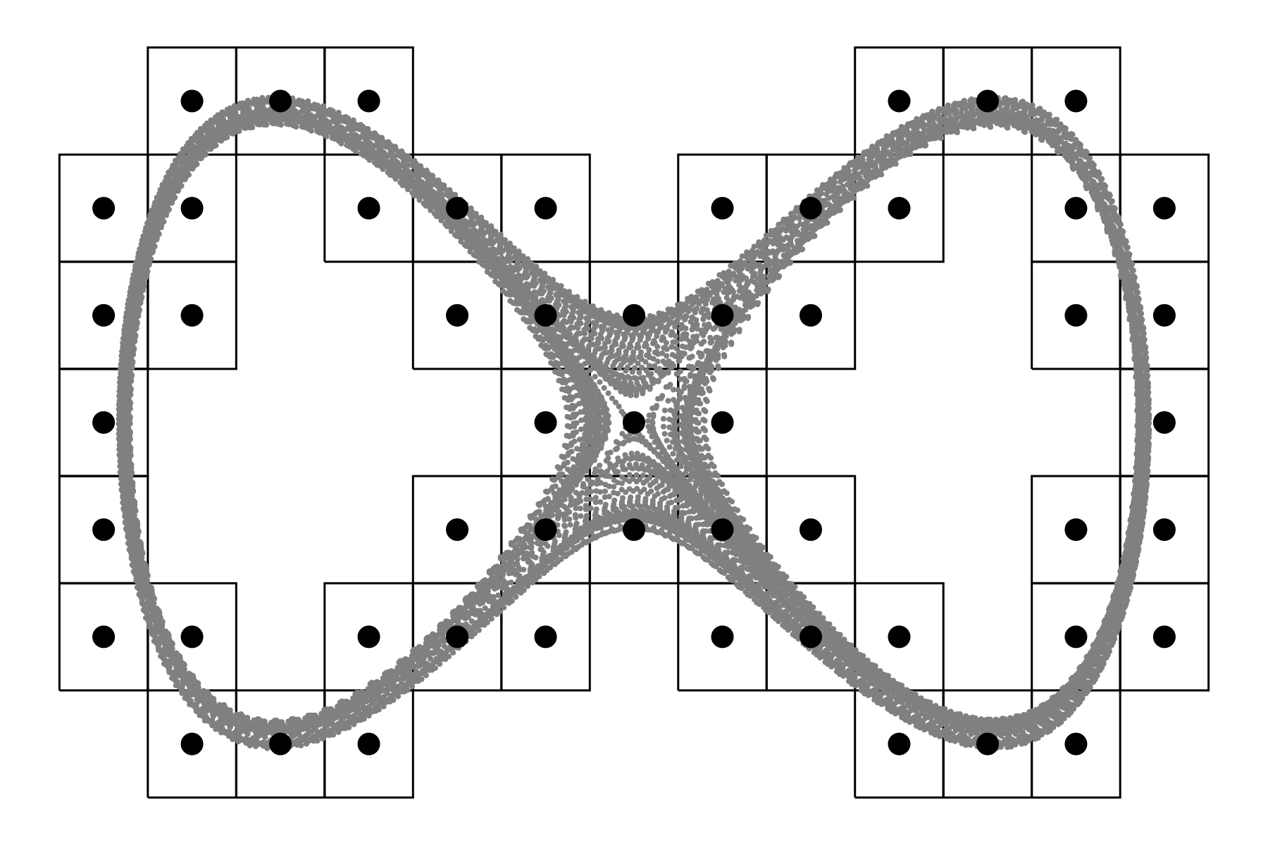

We then resample the time series such that consecutive points lie in different cubes. For this, we set , recursively define
and set , to be the quantization of the time series . Here we let denote the largest finite value of and .
2.2 Coordinates for dynamics
After reviewing the construction of cyclic coordinates from cohomology and how these coordinates are lifted for a time series, we explain how to find elements of that induce dynamically relevant coordinates.
1. Cohomology and circular coordinates.
Given a set of box centers , we construct the Vietoris–Rips complex , where and . Note that the choice of and allows a point in to be connected to all its diagonal neighbors. An example is shown in Fig. 1(b).
Next, we compute a basis of . Using the procedure introduced in [6], a circle valued coordinate can be constructed for each generator in . More precisely, as a function on the vertices, the coordinate can be chosen as any solution of the optimization problem
composed with the canonical projection . Here denotes the coboundary operator, is the sum of over all edges in and is any 1-cocycle in the respective coset. We remark that does not depend on the choice of and is unique up to an additive constant on each connected component of .
The set of coordinates however does depend on the choice of the basis . As an example, consider the complex in Fig. 1(b). Since its first cohomology group is isomorphic to , each basis consists of two cocycles. Figures 2 and 3 show coordinates for two different bases. The problem of choosing a suitable basis is addressed in a later section.


2. Lifted Coordinates.
Given a quantized time series and a circular coordinate we can form the composite , which captures the change of the coordinate over time. Analogous to continuous maps, we lift this function to a function such that : We define the lifted coordinate of and via and
where denotes the signed geodesic distance from to on . Figure 4 shows an example for a coordinate and its lift.


3. Dynamically Relevant Coordinates
We now identify coordinates which are relevant for dynamics. This is done in three steps: First, we define the correlation of coordinates which is large if coordinates describe the same features of the dynamics. Second, we search for a correlation-minimal basis of . Finally, we discard all coordinates from this basis which do not describe any cycling dynamics.
We begin by defining the correlation number of two lifted coordinates and as
| (1) |
where the -th entry of the vector is the forward finite difference and denotes the standard Euclidean scalar product. For a basis of we define its correlation number as
| (2) |
These definitions can be motivated as follows: If two coordinates are to describe different features of the dynamics of a time series, they should change at disjoint periods of time, this is measured in (1). For an optimal basis, we therefore minimize the overall correlation which is written out in (2).
As an example, we again consider the time series 1(a). From Fig. 4(b) we know that for the first time steps, the series does turns around the right hole. Now consider Fig. 5 where the lifted coordinates for the generating sets of figures Fig. 2 and Fig. 3 are plotted for the first time steps. The plots indicates that the lifted coordinates in Fig. 5(a) have a lower correlation number than the ones in Fig. 5(b). An explicit computation (for all time steps) yields the values and , respectively, confirming that the preferred basis has lower correlation.


We now search for a basis with minimal correlation. Assuming is any basis for the free group , every basis can be written as where . In order to find a correlation minimizing basis, we search , starting with the identity and recursively applying basis change operations (sums/swaps of rows/columns, multiplication of rows/columns with a unit) to up to a given depth. Of all these matrices we return the one with minimal correlation.
This approach works sufficiently well for simple examples. However, since we are only searching a finite subset of we have no guarantee of actually finding a minimizer (if one even exists). A better algorithm for finding a correlation minimal basis is a topic for future work.
At this point, the set contains many coordinates. Since the mere presence of a -cycle does not imply the existence of cycling motion around the corresponding coordinate, we have to identify those coordinates in which capture cycling behavior. For this, note that whenever the function is monotonic on some interval , the trajectory is moving along the cyclic coordinate . We define the time series to be cycling along if there is an interval where satisfies a monotonicity criterion and . The second condition ensures that the time series completes at least one full turn during the segment . For a monotonicity criterion, a possible choice is
for all and a fixed .
is then said to be -increasing along . In practice, we slightly relax this criterion and only require since sometimes adjacent cubes get assigned the exact same coordinate value. In this case, is said to be almost -increasing on . Note that the parameter has to be specified by the user; we typically do this by inspecting the lifted coordinates.
We define the subset of all dynamically relevant generators of the basis as all for which the time series is cycling along . The elements in will be called spurious generators.
2.3 Macro model
We transfer the information on cycling motion back to the cubical covering: A cube in the covering is -cycling if the trajectory is cycling along on some interval and there is such that . For , let be the set of all dynamically relevant generators for which is -cycling.
The cubical covering can now be decomposed into equivalence classes: Two cubes are equivalent if they are cycling with respect to the same set of non-spurious generators of :
We can furthermore distinguish cubes in which the trajectory ceases to be cycling. For this, assume the time series is -cycling along an interval which is maximal in the sense that the time series is not -cycling on any interval which contains . Now let be the first time step such that . Then the cubes are precisely those cubes which are hit during the last full turn with respect to in . We call such cubes -transient. For a given cube , we let denote the set of all generators which is transient for.
As a finer classification of cubes we can define
We now classify the cubes in according to either of these two equivalence relations and count transitions between the classes. That is, we build the quotient
as well as the transition matrix
We now call a macro model, and an extended macro model for the given time series.

| 1161 | 45 | 47 | -trn | |
| 1264 | 55 | 49 | -trn | |
| 44 | 56 | 35 | -trn -trn | |
| 47 | 49 | no cycling |

| 4 | -cyc | |||||
| 4 | 1256 | 55 | 49 | -trn | ||
| 4 | -cyc | |||||
| 4 | 1153 | 45 | 47 | -trn | ||
| 56 | 44 | 35 | -trn -trn | |||
| 49 | 47 | no cycling |
We remark that by rescaling the columns of one obtains a Markov matrix with entries which could be interpreted as transition probabilities between different regions. We deliberately choose not to define transition matrices this way, since transitions generally do not satisfy a Markov property.
3 Experiments
The following results are obtained using our implementation of the pipeline in Section 2 in the programming language Julia [3]. In particular, we use the algorithm in [9] for computing with integer coefficients.
3.1 Perturbed double well
The time series in Fig. 1, which was used to illustrate the constructions in Section 2, was obtained by integrating a stochastically perturbed version of the double well Hamiltonian system
| (3) |
with , , and denoting Brownian motion. We integrate (3) from the initial value by the SRIW1 scheme [14] with step size 0.01.
The macro models in Fig. 6 and Fig. 7 were generated using the coordinates in Fig. 2 and the monotonicity criterion ” is almost -increasing” with . We note that Fig. 5(a) provides a hint for choosing since 3.5 turns in 80 steps average to an increase of approximately per step. These models are like we would expect for such simple dynamics. The yellow boxes capture the location in phase space where direct transitions between the loops is possible and the green and blue boxes capture the location where the trajectory cycles around the natural holes.
3.2 The Lorenz system
For this example we generated a time series by integrating the Lorenz system with the classical parameters and with time step size for million time steps using the classical fourth order Runge Kutta method. As starting value, we choose , but we discard the first 6000 time steps since they ’close up’ the left holes of the complex. This highlights one shortcoming of our current technique which will be addressed in future work.


We choose the quantization radius and construct a cubical covering with 652 cubes and a quantized time series with 42698 points. Since the first cohomology of the resulting Vietoris-Rips complex is two-dimensional, we compute two circular coordinates, which are both seen to be dynamically relevant with the monotonicity criterion ” is almost 0.007-increasing”. Plots for the time series and the intermediate steps can be found in Fig. 8.

| 15925 | 818 | -cycling | ||
| 15011 | 876 | 2 | -cycling | |
| 818 | 875 | 8370 | -cycling & -cycling | |
| 2 | no cycling |
The macro model shown in Fig. 9 nicely captures many important aspects of the dynamics on the Lorenz attractor. We learn that there are (at least) two different types of cycling motion, that each of these occurs in a distinct region in phase space (the blue and green regions), and that these regions intersect (yellow region). We furthermore see that cycling dynamics are present almost everywhere in the box decomposition as there are only 2 non-cycling boxes.

| 4065 | 1000 | 11 | 263 | -cyc | ||||
| 968 | 9892 | 80 | 464 | -trns | ||||
| 2953 | 789 | 222 | 8 | -cyc | ||||
| 701 | 10568 | 92 | 82 | 472 | 2 | -trns | ||
| 366 | 401 | 3133 | 160 | 301 | -trns -trns | |||
| 14 | 106 | 306 | 66 | 452 | 2098 | 33 | -trns -cyc | |
| 292 | 40 | 12 | 90 | 604 | 39 | 1550 | -cyc -trns | |
| 2 | no cycling |
In the extended macro model (Fig. 10), we see that the cycling regions are subdivided into a cycling set near the center of the wings and a transient set near the outside of the wings. This indicates that all cycling dynamics in the inside of the wings eventually moves to the outer regions. The extended model furthermore identifies the regions where direct transitions between cycling dynamics can occur. The purple and yellow regions in Fig. 10(a) are the only regions where a direct transition from - to -cycling dynamics is possible and the orange and yellow regions are the only places that can contain the reverse transition.
4 Discussion
The techniques described in this paper appear to be a promising novel approach to identifying from time series data regions of phase space in which oscillations occur and locations at which transitions between these oscillations occur. However, a number of distinct questions need to be answered to obtain confidence in applying this technique to complicated higher-dimensional systems, where the results cannot be inspected and modified by visualization. We briefly address those in the following paragraphs.
Construction of the complex.
The computation of circle-valued coordinates from data requires the construction of a geometric complex. The approach chosen in this article accomplishes this by constructing a Vietoris–Rips complex from a suitably quantized version of the given time series. In particular, we rely on finding a quantization radius which is small enough to contain those holes which give rise to dynamically relevant coordinates and large enough to connect the data in a meaningful way. In general, such a radius need not exist. This even happens in the Lorenz system with a trajectory that starts very close to the center of one of the wings.
Finding optimal coordinates.
When searching for dynamically relevant coordinates, we encounter the problem of finding a correlation minimizing basis. This poses the natural question of existence and uniqueness of such a basis. In addition, an algorithm is needed to compute this basis or a suitable approximation. Furthermore, since sparse data can lead to a large dimension of , an efficient algorithm for this computation would be desirable. We hope to be able to address this using techniques inspired by those for the computation of (persistent) cohomology with coefficients in a finite field [4].
Identifying cycling motion.
In this contribution, cycling motion is identified by analyzing the monotonicity behavior of circle valued coordinates. While this leads to satisfactory results in the presented examples, we have no general reliable procedure of identifying recurrence. For example, a cycling time series with a bit of back-and-forth moving in every full turn would be difficult to identify using the presented methods.
References
- [1]
- [2] H. Ban and W. D. Kalies. A computational approach to Conley’s decomposition theorem. J. Comp. Nonl. Dyn., 1(4):312–319, 2006.
- [3] J. Bezanson, A. Edelman, S. Karpinski, and V. B. Shah. Julia: A Fresh Approach to Numerical Computing. SIAM Review, 59: 65–98, 2017.
- [4] U. Bauer. Ripser: efficient computation of Vietoris–Rips persistence barcodes. Preprint, arXiv:1908.02518, Aug 2019.
- [5] C. Conley. Isolated invariant sets and the Morse index, volume 38 of CBMS Regional Conference Series in Mathematics. American Mathematical Society, Providence, R.I., 1978.
- [6] V. de Silva, D. Morozov, and M. Vejdemo-Johansson. Persistent Cohomology and Circular Coordinates. Discr. Comp. Geom., 45(4):737–759, 2009.
- [7] M. Dellnitz and O. Junge. On the approximation of complicated dynamical behavior. SIAM J. Numer. Anal., 36(2):491–515, 1999.
- [8] O. Dellnitz, M.; Junge. Set oriented numerical methods for dynamical systems, B. Fiedler, G. Iooss and N. Kopell (eds.), in: Handbook of Dynamical Systems III: Towards Applications. World Scientific, 2002.
- [9] S. Harker, K. Mischaikow, M. Mrozek, and V. Nanda. Discrete Morse theoretic algorithms for computing homology of complexes and maps. Found. Comput. Math., 14(1):151–184, 2014.
- [10] K. Mischaikow. Topological techniques for efficient rigorous computation in dynamics. Acta Numer., 11:435–477, 2002.
- [11] W. D. Kalies, K. Mischaikow, and VanderVorst, R. C. A. M. An algorithmic approach to chain recurrence. Found. Comput. Math., 5(4):409–449, 2005.
- [12] K. Mischaikow, M. Mrozek, and F. Weilandt. Discretization strategies for computing Conley indices and Morse decompositions of flows. J. Comput. Dyn., 3(1):1–16, 2016.
- [13] George Osipenko. Construction of attractors and filtrations. In Conley index theory (Warsaw, 1997), volume 47 of Banach Center Publ., pages 173–192. Polish Acad. Sci. Inst. Math., Warsaw, 1999.
- [14] A. Rößler. Runge-Kutta methods for the strong approximation of solutions of stochastic differential equations. SIAM J. Numer. Anal., 48(3):922–952, 2010.