跳到论文正文
W Papers独立论文阅读器 arXiv:2001.06966 论文正文 计算阅读时间 · 0%
引用这篇论文根据当前论文元数据生成,正式投稿前建议核对。


License: arXiv.org perpetual non-exclusive license
arXiv:2001.06966v3 [math.ST] 29 Sep 2020

Reconciling the Gaussian and Whittle Likelihood with an application to estimation in the frequency domain

Suhasini Subba Rao Note: Texas A&M University, College Station, Texas, TX 77845, U.S.A.    Junho Yang Note: Authors ordered alphabetically
August 11, 2026
Abstract

In time series analysis there is an apparent dichotomy between time and frequency domain methods. The aim of this paper is to draw connections between frequency and time domain methods. Our focus will be on reconciling the Gaussian likelihood and the Whittle likelihood. We derive an exact, interpretable, bound between the Gaussian and Whittle likelihood of a second order stationary time series. The derivation is based on obtaining the transformation which is biorthogonal to the discrete Fourier transform of the time series. Such a transformation yields a new decomposition for the inverse of a Toeplitz matrix and enables the representation of the Gaussian likelihood within the frequency domain. We show that the difference between the Gaussian and Whittle likelihood is due to the omission of the best linear predictions outside the domain of observation in the periodogram associated with the Whittle likelihood. Based on this result, we obtain an approximation for the difference between the Gaussian and Whittle likelihoods in terms of the best fitting, finite order autoregressive parameters. These approximations are used to define two new frequency domain quasi-likelihoods criteria. We show that these new criteria can yield a better approximation of the spectral divergence criterion, as compared to both the Gaussian and Whittle likelihoods. In simulations, we show that the proposed estimators have satisfactory finite sample properties.

Keywords and phrases: Biorthogonal transforms, discrete Fourier transform, periodogram, quasi-likelihoods and second order stationary time series.

1 Introduction

In his seminal work, Whittle (1951, 1953) introduced the Whittle likelihood as an approximation of the Gaussian likelihood. A decade later, the asymptotic sampling properties of moving average models fitted using the Whittle likelihood were derived in Walker 1964. Subsequently, the Whittle likelihood has become a popular method for parameter estimation of various stationary time series (both long and short memory) and spatial models. The Whittle likelihood is computationally a very attractive method for estimation. Despite the considerable improvements in technology, interest in the Whittle likelihood has not abated. The Whittle likelihood has gained further traction as a quasi-likelihood (or as an information criterion, see Parzen 1983) between the periodogram and the spectral density. Several diverse applications of the Whittle likelihood can be found in Fox and Taqqu 1986, Dahlhaus and Künsch 1987 (for spatial processes), Robinson 1995, Dahlhaus 2000, Hurvich and Chen 2000, Giraitis and Robinson 2001, Choudhuri et al. 2004, Abadir et al. 2007, Shao and Wu 2007, Giraitis et al. 2012 (long memory time series and local Whittle methods), Panaretos and Tavakoli 2013, Kirch et al. 2019 (Bayesian spectral methods), and van Delft and Eichler 2020 (functional time series), to name but a few.

Despite its advantages, it is well known that for small samples the Whittle likelihood can give rise to estimators with a substantial bias (see Priestley 1981 and Dahlhaus 1988). Dahlhaus 1988 shows that the finite sample bias in the periodogram impacts the performance of the Whittle likelihood. Motivated by this discrepancy, Sykulski et al. 2019 proposes the debiased Whittle likelihood, which fits directly to the expectation of the periodogram rather than the limiting spectral density. Alternatively, Dahlhaus 1988 shows that the tapered periodogram is better at capturing the features in the spectral density, such as peaks, than the regular periodogram. He uses this as the basis of the tapered Whittle likelihood. Empirical studies show that the tapered Whittle likelihood yields a smaller bias than the regular Whittle likelihood. As a theoretical justification, Dahlhaus (1988, 1990) uses an alternative asymptotic framework to show that tapering yields a good approximation to the inverse of the Toeplitz matrix. It is worth mentioning that within the time domain, several authors, including Shaman (1975, 1976), Bhansali 1982 and Coursol and Dacunha-Castelle 1982, have studied approximations to the inverse of the Toeplitz matrix. These results can be used to approximate the Gaussian likelihood.

However, as far as we are aware, there are no results which explain what is lost when using the Whittle likelihood rather than the Gaussian likelihood. The objective of this paper is to address some of these issues. The benefits of such insights are not only of theoretical interest but also lead to the development of computationally simple frequency domain methods which are comparable with the Gaussian likelihood.

We first recall the definition of the Gaussian and Whittle likelihood. Our aim is to fit a parametric second order stationary model with spectral density fθ​(ω)f_{\theta}(\omega) and corresponding autocovariance function {cfθ​(r)}r∈ℤ\{c_{f_{\theta}}(r)\}_{r\in\mathbb{Z}} to the observed time series {Xt}t=1n\{X_{t}\}_{t=1}^{n}. The (quasi) log-Gaussian likelihood is proportional to

ℒn​(θ,X¯n)=n−1​(X¯n′​Γn​(fθ)−1​X¯n+log⁡|Γn​(fθ)|)\mathcal{L}_{n}(\theta;\underline{X}_{n})=n^{-1}\left(\underline{X}_{n}^{\prime}\Gamma_{n}(f_{\theta})^{-1}\underline{X}_{n}+\log|\Gamma_{n}(f_{\theta})|\right) (1.1)

where Γn​(fθ)s,t=cfθ​(s−t)\Gamma_{n}(f_{\theta})_{s,t}=c_{f_{\theta}}(s-t), |A||A| denotes the determinant of the matrix AA and X¯n′=(X1,…,Xn)\underline{X}_{n}^{\prime}=(X_{1},\ldots,X_{n}). In contrast, the Whittle likelihood is a “spectral divergence” between the periodogram and the candidate spectral density. There are two subtly different methods for defining this contrast, one is with an integral the other is to use the Riemann sum. In this paper, we focus on the Whittle likelihood defined in terms of the Riemann sum over the fundamental frequencies

Kn​(θ,X¯n)=n−1​∑k=1n(|Jn​(ωk,n)|2fθ​(ωk,n)+log⁡fθ​(ωk,n))ωk,n=2​π​kn,K_{n}(\theta;\underline{X}_{n})=n^{-1}\sum_{k=1}^{n}\left(\frac{|J_{n}(\omega_{k,n})|^{2}}{f_{\theta}(\omega_{k,n})}+\log f_{\theta}(\omega_{k,n})\right)\quad\omega_{k,n}=\frac{2\pi k}{n}, (1.2)

where Jn(ωk,n)=n−1/2∑t=1nXtei​t​ωk,nJ_{n}(\omega_{k,n})=n^{-1/2}\sum_{t=1}^{n}X_{t}e^{it\omega_{k,n}} is the discrete Fourier transform (DFT) of the observed time series. To compare the Gaussian and Whittle likelihood, we rewrite the Whittle likelihood in matrix form. We define the n×nn\times n circulant matrix Cn​(fθ)C_{n}(f_{\theta}) with entries (Cn​(fθ))s,t=n−1​∑k=1nfθ​(ωk,n)​e−i⁡(s−t)​ωk,n(C_{n}(f_{\theta}))_{s,t}=n^{-1}\sum_{k=1}^{n}f_{\theta}(\omega_{k,n})e^{-i(s-t)\omega_{k,n}}. The Whittle likelihood Kn​(θ,X¯n)K_{n}(\theta;\underline{X}_{n}) can be written as

Kn​(θ,X¯n)=n−1​(X¯n′​Cn​(fθ−1)​X¯n+∑k=1nlog⁡fθ​(ωk,n)).K_{n}(\theta;\underline{X}_{n})=n^{-1}\left(\underline{X}_{n}^{\prime}C_{n}(f_{\theta}^{-1})\underline{X}_{n}+\sum_{k=1}^{n}\log f_{\theta}(\omega_{k,n})\right). (1.3)

To obtain an exact expression for Γn​(fθ)−1−Cn​(fθ−1)\Gamma_{n}(f_{\theta})^{-1}-C_{n}(f_{\theta}^{-1}) and X¯n′​[Γn​(fθ)−1−Cn​(fθ−1)]​X¯n\underline{X}^{\prime}_{n}[\Gamma_{n}(f_{\theta})^{-1}-C_{n}(f_{\theta}^{-1})]\underline{X}_{n}, we focus on the DFT of the time series. The idea is to obtain the linear transformation of the observed time series {Xt}t=1n\{X_{t}\}_{t=1}^{n} which is biorthogonal to the regular DFT, {Jn​(ωk,n)}k=1n\{J_{n}(\omega_{k,n})\}_{k=1}^{n}. The biorthogonal transform, when coupled with the regular DFT, exactly decorrelates the time series. In Section 2.3, we show that the biorthogonal transform corresponding to the regular DFT contains the regular DFT plus the Fourier transform of the best linear predictors of the time series outside the domain of observation. Since this transformation completes the information not found in the regular DFT, we call it the complete DFT. It is common to use the Cholesky decomposition to decompose the inverse of a Toeplitz matrix. An interesting aspect of the biorthogonal transformation is that it provides an alternative decomposition of the inverse of a Toeplitz matrix.

In Section 2.4, we show that the complete DFT, together with the regular DFT, allows us to rewrite the Gaussian likelihood within the frequency domain (which, as far as we are aware, is new). Further, it is well known that the Whittle likelihood has a bias due to the boundary effect. By rewriting the Gaussian likelihood within the frequency domain we show that the Gaussian likelihood avoids the boundary effect problem by predicting the time series outside the domain of observation. Precisely, the approximation error between the Gaussian and Whittle likelihood is due to the omission of these linear predictors in the regular DFT. From this result, we observe that the greater the persistence in the time series model (which corresponds to a more peaked spectral density) the larger the loss in approximating the complete DFT with the regular DFT. In order to obtain a better approximation of the Gaussian likelihood in the frequency domain, it is of interest to approximate the difference of the two likelihoods ℒn​(θ,X¯n)−Kn​(θ,X¯n)\mathcal{L}_{n}(\theta;\underline{X}_{n})-K_{n}(\theta;\underline{X}_{n}). For autoregressive processes of finite order, we obtain an analytic expression for the difference in the two likelihoods in terms of the AR parameters (see equation (2.21)). For general second order stationary models, the expression is more complex. In Section 3, we obtain an approximation for ℒn​(θ,X¯n)−Kn​(θ,X¯n)\mathcal{L}_{n}(\theta;\underline{X}_{n})-K_{n}(\theta;\underline{X}_{n}) in terms of the infinite order (causal/minimum phase) autoregressive factorisation of fθ​(ω)=σ2​|1−∑j=1∞ϕj​e−i​j​ω|−2f_{\theta}(\omega)=\sigma^{2}|1-\sum_{j=1}^{\infty}\phi_{j}e^{-ij\omega}|^{-2}. We show that this approximation is the first order term in a series expansion of the inverse of the Toeplitz matrix, Γn​(f)−1\Gamma_{n}(f)^{-1}. More precisely, in Section 3.2, we show that Γn​(f)−1\Gamma_{n}(f)^{-1} can be expressed in terms of Cn​(fθ)−1C_{n}(f_{\theta})^{-1} plus a polynomial-type series expansion of the AR(∞)(\infty) coefficients.

In Section 4, we obtain an approximation for the difference ℒn​(θ,X¯n)−Kn​(θ,X¯n)\mathcal{L}_{n}(\theta;\underline{X}_{n})-K_{n}(\theta;\underline{X}_{n}) in terms of a finite order autoregressive process. We use this to define two spectral divergence criteria which are “almost” unbiased estimators of the spectral divergence between the true (underlying spectral) density and the parametric spectral density. We use these criteria to define two new frequency domain estimators. In Section 5, we obtain the asymptotic sampling properties of the new likelihood estimators including the asymptotic bias and variance. Finally, in Section 6, we illustrate and compare the proposed frequency domain estimators through some simulations. We study the performance of the estimation scheme when the parametric model is both correctly specified and misspecified.

The proofs can be found in the Supplementary material. The main proofs can be found in Appendix A, B, D and E. Baxter type inequalities for derivatives of finite predictors can be found in Appendix C. These results are used to obtain an approximation for the difference between the derivatives of the Gaussian and Whittle likelihood. In Appendix E we derive an expression for the asymptotic bias of the Gaussian, Whittle likelihoods, and the new frequency domain likelihoods, described above. In Appendix F, G and H we present additional simulations.

2 The Gaussian likelihood in the frequency domain

2.1 Preliminaries

In this section, we introduce most of the notation used in the paper, it can be skipped on first reading. To reduce notation, we omit the symbol X¯n\underline{X}_{n} in the Gaussian and Whittle likelihood. Moreover, since the focus in this paper will be on the first terms in the Gaussian and Whittle likelihoods we use ℒn​(θ)\mathcal{L}_{n}(\theta) and Kn​(θ)K_{n}(\theta) to denote only these terms:

ℒn​(θ)=n−1​X¯n′​Γn​(fθ)−1​X¯nandKn​(θ)=n−1​X¯n′​Cn​(fθ−1)​X¯n.\mathcal{L}_{n}(\theta)=n^{-1}\underline{X}_{n}^{\prime}\Gamma_{n}(f_{\theta})^{-1}\underline{X}_{n}\quad\textrm{and}\quad K_{n}(\theta)=n^{-1}\underline{X}_{n}^{\prime}C_{n}(f_{\theta}^{-1})\underline{X}_{n}. (2.1)

Let A∗A^{*} denote the conjugate transpose of the matrix AA. We recall that the circulant matrix Cn​(g)C_{n}(g) can be written as Cn​(g)=Fn∗​Δn​(g)​FnC_{n}(g)=F_{n}^{*}\Delta_{n}(g)F_{n}, where Δn​(g)=diag⁡(g⁡(ω1,n),…,g⁡(ωn,n))\Delta_{n}(g)=\mathrm{diag}(g(\omega_{1,n}),\ldots,g(\omega_{n,n})) (diagonal matrix) and FnF_{n} is the n×nn\times n DFT matrix with entries (Fn)k,t=n−1/2ei​t​ωk,n(F_{n})_{k,t}=n^{-1/2}e^{it\omega_{k,n}}. We recall that the eigenvalues and the corresponding eigenvectors of any circulant matrix Cn​(g)C_{n}(g) are {g⁡(ωk,n)}k=1n\{g(\omega_{k,n})\}_{k=1}^{n} and {e¯k,n′=(ei​k​ω1,n,…,ei​k​ωn,n)}k=1n\{\underline{e}_{k,n}^{\prime}=(e^{ik\omega_{1,n}},\ldots,e^{ik\omega_{n,n}})\}_{k=1}^{n} respectively.

In general, we assume that 𝔼⁡[Xt]=0\mathbb{E}[X_{t}]=0 (as it makes the derivations cleaner). We use {cf​(r)}r∈ℤ\{c_{f}(r)\}_{r\in\mathbb{Z}} to denote an autocovariance function and f⁡(ω)=∑r∈ℤcf​(r)​ei​r​ωf(\omega)=\sum_{r\in\mathbb{Z}}c_{f}(r)e^{ir\omega} its corresponding spectral density. Sometimes, it will be necessary to make explicit the true underlying covariance (equivalently the spectral density) of the process. In this case, we use the notation covf​(Xt,Xt+r)=𝔼f​[Xt​Xt+r]=cf​(r)\mathrm{cov}_{f}(X_{t},X_{t+r})=\mathbb{E}_{f}[X_{t}X_{t+r}]=c_{f}(r). Next we define the norms we will use. Suppose AA is a n×nn\times n square matrix, let ‖A‖p=(∑i,j=1n|ai,j|p)1/p\|A\|_{p}=(\sum_{i,j=1}^{n}|a_{i,j}|^{p})^{1/p} be an entrywise pp-norm for p≥1p\geq 1, and ‖A‖s​p​e​c\|A\|_{spec} denote the spectral norm. Let ‖X‖𝔼,p=(𝔼​|X|p)1/p\|X\|_{\mathbb{E},p}=\left(\mathbb{E}|X|^{p}\right)^{1/p}, where XX is a random variable. For the 2​π2\pi-periodic square integrable function gg with g⁡(ω)=∑r∈ℤgr​ei​r​ωg(\omega)=\sum_{r\in\mathbb{Z}}g_{r}e^{ir\omega}, we use the sub-multiplicative norm ‖g‖K=∑r∈ℤ(2K+|r|K)​|gr|\|g\|_{K}=\sum_{r\in\mathbb{Z}}(2^{K}+|r|^{K})|g_{r}|. Note that if ∑j=0K+2supω|g(j)​(ω)|<∞\sum_{j=0}^{K+2}\sup_{\omega}|g^{(j)}(\omega)|<\infty then ‖g‖K<∞\|g\|_{K}<\infty, where g(j)​(⋅)g^{(j)}(\cdot) denotes the jjth derivative of gg.

Suppose f,g:[0,2​π]→ℝf,g:[0,2\pi]\rightarrow\mathbb{R} are bounded functions, that are strictly larger than zero and are symmetric about π\pi. By using the classical factorisation results in Szegö 1921 and Baxter 1962 we can write f⁡(⋅)=σf2​|ψf​(⋅)|2=σf2​|ϕf​(⋅)|−2f(\cdot)=\sigma_{f}^{2}|\psi_{f}(\cdot)|^{2}=\sigma^{2}_{f}|\phi_{f}(\cdot)|^{-2}, where ϕf​(ω)=1−∑j=1∞ϕj​(f)​e−i​j​ω\phi_{f}(\omega)=1-\sum_{j=1}^{\infty}\phi_{j}(f)e^{-ij\omega} and ψf​(ω)=1+∑j=1∞ψj​(f)​e−i​j​ω\psi_{f}(\omega)=1+\sum_{j=1}^{\infty}\psi_{j}(f)e^{-ij\omega}, the terms σg\sigma_{g}, ϕg​(⋅)\phi_{g}(\cdot), and ψg​(⋅)\psi_{g}(\cdot) are defined similarly. We use these expansions in Sections 3 and 4, where we require the following notation

ρn,K​(f)\displaystyle\rho_{n,K}(f) =\displaystyle= ∑r=n+1∞|rK​ϕr​(f)|,\displaystyle\sum_{r=n+1}^{\infty}|r^{K}\phi_{r}(f)|,
AK​(f,g)\displaystyle A_{K}(f,g) =\displaystyle= 2​σg−2​‖ψf‖0​‖ϕg‖02​‖ϕf‖K,\displaystyle 2\sigma_{g}^{-2}\|\psi_{f}\|_{0}\|\phi_{g}\|_{0}^{2}\|\phi_{f}\|_{K},
andCf,K\displaystyle\textrm{and}\qquad C_{f,K} =\displaystyle= 3−ε1−ε​‖ϕf‖K2​‖ψf‖K2\displaystyle\frac{3-\varepsilon}{1-\varepsilon}\left\|\phi_{f}\right\|_{K}^{2}\left\|\psi_{f}\right\|_{K}^{2}

for some 0<ε<10<\varepsilon<1.

For postive sequences {an}\{a_{n}\} and {bn}\{b_{n}\}, we denote an∼bna_{n}\sim b_{n} if there exist 0<C1≤C2<∞0<C_{1}\leq C_{2}<\infty such that C1≤an/bn≤C2C_{1}\leq a_{n}/b_{n}\leq C_{2} for all nn. Lastly, we denote Re\operatorname{Re} and Im\operatorname{Im} as the real and imaginary part of a complex variable respectively.

2.2 Motivation

In order to motivate our approach, we first study the difference in the bias of the AR(1)(1) parameter estimator using both the Gaussian and Whittle likelihood. In Figure 1, we plot the bias in the estimator of ϕ\phi in the AR(1)(1) model Xt=ϕ​Xt−1+εtX_{t}=\phi X_{t-1}+\varepsilon_{t} for different values of ϕ\phi (based on sample size n=20n=20). We observe that the difference between the bias of the two estimators increases as |ϕ||\phi| approaches one. Further, the Gaussian likelihood clearly has a smaller bias than the Whittle likelihood (which is more pronounced when |ϕ||\phi| is close to one).

Figure 1: The model Xt=ϕ​Xt−1+εtX_{t}=\phi X_{t-1}+\varepsilon_{t} with independent standard normal errors is simulated. The bias of the estimator of ϕ\phi based on sample size n=20n=20 over 1000 replications.

Let {Xt}t=1n\{X_{t}\}_{t=1}^{n} denote the observed time series. Straightforward calculations (based on expressions for Γn​(fϕ)−1\Gamma_{n}(f_{\phi})^{-1} and Cn​(fϕ−1)C_{n}(f_{\phi}^{-1})) show that the difference between the Gaussian and Whittle likelihoods for an AR(1)(1) model is

ℒn​(ϕ)−Kn​(ϕ)=n−1​[2​ϕ​X1​Xn−ϕ2​(X12+Xn2)]\mathcal{L}_{n}(\phi)-K_{n}(\phi)=n^{-1}\left[2\phi X_{1}X_{n}-\phi^{2}(X_{1}^{2}+X_{n}^{2})\right] (2.2)

Thus we observe that the closer |ϕ||\phi| is to one, the larger the expected difference between the likelihoods. Using (2.2) and the Bartlett correction (see Bartlett 1953 and Cox and Snell 1968, it is possible to obtain an asymptotic expression for the difference in the biases (see also Appendix E.2) Generalisations of this result to higher order AR(p)(p) models may also be possible using the analytic expression for the inverse of the Toeplitz matrix corresponding to an AR(p)(p) model derived in Siddiqui 1958 and Galbraith and Galbraith 1974.

However, for more general models, such as the MA(q)(q) or ARMA(p,q)(p,q) models, using brute force calculations for deriving the difference ℒn​(θ)−Kn​(θ)\mathcal{L}_{n}(\theta)-K_{n}(\theta) and its derivatives is extremely difficult. Furthermore, such results do not offer any insight on how the Gaussian and Whittle likelihood are related, nor what is “lost” when going from the Gaussian likelihood to the Whittle likelihood. In the remainder of this section, we derive an exact expression for the Gaussian likelihood in the frequency domain. Using these derivations, we obtain a simple expression for the difference between the Whittle and Gaussian likelihood for AR(p)(p) models. In subsequent sections, we obtain approximations for this difference for general time series models.

2.3 The biorthogonal transform to the discrete Fourier transform

In order to obtain an exact bound, we start with the Whittle likelihood and recall that the DFT of the time series plays a fundamental role in its formulation. With this in mind, our approach is based on deriving the transformation {Zk,n}k=1n⊂sp⁡(X¯n)\{Z_{k,n}\}_{k=1}^{n}\subset\mathrm{sp}(\underline{X}_{n}) (where sp⁡(X¯n)\mathrm{sp}(\underline{X}_{n}) denotes the linear space over a complex field spanned by X¯n={Xt}t=1n\underline{X}_{n}=\{X_{t}\}_{t=1}^{n}), which is biorthogonal to {Jn​(ωk,n)}k=1n\{J_{n}(\omega_{k,n})\}_{k=1}^{n}. That is, we derive a transformation {Zk,n}k=1n\{Z_{k,n}\}_{k=1}^{n} which when coupled with {Jn​(ωk,n)}k=1n\{J_{n}(\omega_{k,n})\}_{k=1}^{n} satisfies the following condition

covf​(Zk1,n,Jn​(ωk2,n))=f⁡(ωk1)​δk1,k2\mathrm{cov}_{f}\left(Z_{k_{1},n},J_{n}(\omega_{k_{2},n})\right)=f(\omega_{k_{1}})\delta_{k_{1},k_{2}}

where δk1,k2=1\delta_{k_{1},k_{2}}=1 if k1=k2k_{1}=k_{2} (and zero otherwise). Since Z¯n′=(Z1,n,…,Zn,n)∈sp​(X¯n)n\underline{Z}_{n}^{\prime}=(Z_{1,n},\ldots,Z_{n,n})\in\mathrm{sp}(\underline{X}_{n})^{n}, there exists an n×nn\times n complex matrix UnU_{n}, such that Z¯n=Un​X¯n\underline{Z}_{n}=U_{n}\underline{X}_{n}. Since (Jn​(ωk,1),…,Jn​(ωn,n))′=Fn​X¯n(J_{n}(\omega_{k,1}),\ldots,J_{n}(\omega_{n,n}))^{\prime}=F_{n}\underline{X}_{n}, the biorthogonality of Un​X¯nU_{n}\underline{X}_{n} and Fn​X¯nF_{n}\underline{X}_{n} gives covf​(Un​X¯n,Fn​X¯n)=Δn​(f)\mathrm{cov}_{f}\left(U_{n}\underline{X}_{n},F_{n}\underline{X}_{n}\right)=\Delta_{n}(f). The benefit of biorthogonality is that it leads to the following simple identity on the inverse of the variance matrix.

Lemma 2.1

Suppose that UnU_{n} and VnV_{n} are invertible matrices which are biorthogonal with respect to the variance matrix var⁡(X¯n)\mathrm{var}(\underline{X}_{n}). That is cov⁡(Un​X¯n,Vn​X¯n)=Δn\mathrm{cov}(U_{n}\underline{X}_{n},V_{n}\underline{X}_{n})=\Delta_{n}, where Δn\Delta_{n} is a diagonal matrix. Then

var​(X¯n)−1=Vn∗​Δn−1​Un.\mathrm{var}(\underline{X}_{n})^{-1}=V_{n}^{*}\Delta_{n}^{-1}U_{n}. (2.3)

PROOF. It follows immediately from cov⁡(Un​X¯n,Vn​X¯n)=Un​var​(X¯n)​Vn∗=Δn\mathrm{cov}(U_{n}\underline{X}_{n},V_{n}\underline{X}_{n})=U_{n}\mathrm{var}(\underline{X}_{n})V_{n}^{*}=\Delta_{n} and var⁡(X¯n)=Un−1​Δn​(Vn∗)−1\mathrm{var}(\underline{X}_{n})=U_{n}^{-1}\Delta_{n}(V_{n}^{*})^{-1}. □\Box

To understand how Un​X¯nU_{n}\underline{X}_{n} is related to Fn​X¯nF_{n}\underline{X}_{n} we rewrite Un=Fn+Dn​(f)U_{n}=F_{n}+D_{n}(f). We show in the following theorem that Dn​(f)D_{n}(f) has a specific form with an intuitive interpretation. In order to develop these ideas, we use methods from linear prediction. In particular, we define the best linear predictor of XτX_{\tau} for τ≤0\tau\leq 0 and τ>n\tau>n given {Xt}t=1n\{X_{t}\}_{t=1}^{n} as

X^τ,n=∑t=1nϕt,n​(τ,f)​Xt,\widehat{X}_{\tau,n}=\sum_{t=1}^{n}\phi_{t,n}(\tau;f)X_{t}, (2.4)

where {ϕt,n​(τ,f)}t=1n\{\phi_{t,n}(\tau;f)\}_{t=1}^{n} are the coefficients which minimize the L2L_{2}-distance 𝔼f​[Xτ−∑t=1nϕt,n​(τ,f)​Xt]2\mathbb{E}_{f}[X_{\tau}-\sum_{t=1}^{n}\phi_{t,n}(\tau;f)X_{t}]^{2}. Using this notation we obtain the following theorem.

Theorem 2.1 (The biorthogonal transform)

Let {Xt}\{X_{t}\} be a second order stationary, zero mean time series with spectral density ff which is bounded away from zero and whose autocovariance satisfies ∑r∈ℤ|r​cf​(r)|<∞\sum_{r\in\mathbb{Z}}|rc_{f}(r)|<\infty. Let X^τ,n\widehat{X}_{\tau,n} denote the best linear predictors of XτX_{\tau} as defined in (2.4) and {ϕt,n​(τ,f)}t=1n\{\phi_{t,n}(\tau;f)\}_{t=1}^{n} the corresponding coefficients. Then

covf​((Fn+Dn​(f))​X¯n,Fn​X¯n)=Δn​(f),\mathrm{cov}_{f}\big((F_{n}+D_{n}(f))\underline{X}_{n},F_{n}\underline{X}_{n}\big)=\Delta_{n}(f), (2.5)

where Dn​(f)D_{n}(f) has entries

Dn(f)k,t=n−1/2∑τ≤0(ϕt,n(τ;f)ei​τ​ωk,n+ϕn+1−t,n(τ;f)e−i⁡(τ−1)​ωk,n),D_{n}(f)_{k,t}=n^{-1/2}\sum_{\tau\leq 0}\left(\phi_{t,n}(\tau;f)e^{i\tau\omega_{k,n}}+\phi_{n+1-t,n}(\tau;f)e^{-i(\tau-1)\omega_{k,n}}\right), (2.6)

for 1≤k,t≤n1\leq k,t\leq n. And, entrywise 1≤k1,k2≤n1\leq k_{1},k_{2}\leq n, we have

covf​(J~n​(ωk1,n,f),Jn​(ωk2,n))=f⁡(ωk1,n)​δk1,k2\mathrm{cov}_{f}\left(\widetilde{J}_{n}(\omega_{k_{1},n};f),J_{n}(\omega_{k_{2},n})\right)=f(\omega_{k_{1},n})\delta_{k_{1},k_{2}} (2.7)

where J~n​(ω,f)=Jn​(ω)+J^n​(ω,f)\widetilde{J}_{n}(\omega;f)=J_{n}(\omega)+\widehat{J}_{n}(\omega;f) and

J^n(ω;f)=n−1/2∑τ≤0X^τ,nei​τ​ω+n−1/2∑τ>nX^τ,nei​τ​ω.\widehat{J}_{n}(\omega;f)=n^{-1/2}\sum_{\tau\leq 0}\widehat{X}_{\tau,n}e^{i\tau\omega}+n^{-1/2}\sum_{\tau>n}\widehat{X}_{\tau,n}e^{i\tau\omega}. (2.8)

PROOF. See Appendix A (note that identity (2.7) can be directly verified using results on best linear predictors). □\Box

Corollary 2.1 (Inverse Toeplitz identity)

Let Γn​(f)\Gamma_{n}(f) denote an n×nn\times n Toeplitz matrix generated by the spectral density ff. Then equations (2.3) and (2.5) yield the following identity

Γn​(f)−1=Fn∗​Δn​(f−1)​(Fn+Dn​(f)),\displaystyle\Gamma_{n}(f)^{-1}=F_{n}^{*}\Delta_{n}(f^{-1})(F_{n}+D_{n}(f)), (2.9)

where Dn​(f)D_{n}(f) is defined in (2.6). Observe that two spectral density functions f1​(ω)f_{1}(\omega) and f2​(ω)f_{2}(\omega) with the same autocovariance up to lag (n−1)(n-1), {c⁡(r)}r=0n−1\{c(r)\}_{r=0}^{n-1}, can give rise to two different representations

Γn​(f1)−1=Fn∗​Δn​(f1−1)​(Fn+Dn​(f1))=Fn∗​Δn​(f2−1)​(Fn+Dn​(f2))=Γn​(f2)−1.\Gamma_{n}(f_{1})^{-1}=F_{n}^{*}\Delta_{n}(f_{1}^{-1})(F_{n}+D_{n}(f_{1}))=F_{n}^{*}\Delta_{n}(f_{2}^{-1})(F_{n}+D_{n}(f_{2}))=\Gamma_{n}(f_{2})^{-1}.

What we observe is that the biorthogonal transformation (Fn+Dn​(f))​X¯n(F_{n}+D_{n}(f))\underline{X}_{n} extends the domain of observation by predicting outside the boundary. A visualisation of the observations and the predictors that are involved in the construction of J~n​(ω,f)\widetilde{J}_{n}(\omega;f) is given in Figure 2.

Refer to caption
Figure 2: J~n​(ω,f)\widetilde{J}_{n}(\omega;f) is the Fourier transform over both the observed time series and its predictors outside this domain.

It is quite surprising that only a small modification of the regular DFT leads to its biorthogonal transformation. Furthermore, the contribution of the additional DFT term is J^n(ωk,n;f)=Op(n−1/2)\widehat{J}_{n}(\omega_{k,n};f)=O_{p}(n^{-1/2}). This is why the regular DFT satisfies the well known “near” orthogonal property

covf​(Jn​(ωk1,n),Jn​(ωk2,n))=f⁡(ωk1)​δk1,k2+O⁡(n−1),\mathrm{cov}_{f}(J_{n}(\omega_{k_{1},n}),J_{n}(\omega_{k_{2},n}))=f(\omega_{k_{1}})\delta_{k_{1},k_{2}}+O(n^{-1}),

see Lahiri 2003 and Brillinger 2001. For future reference, we will use the following definitions.

Definition 2.1

We refer to J^n​(ω,f)\widehat{J}_{n}(\omega;f) as the predictive DFT (as it is the Fourier transform of all the linear predictors), noting that basic algebra yields the expression

J^n(ω;f)=n−1/2∑t=1nXt∑τ≤0(ϕt,n(τ;f)ei​τ​ω+ei​n​ωϕn+1−t,n(τ;f)e−i⁡(τ−1)​ω).\widehat{J}_{n}(\omega;f)=n^{-1/2}\sum_{t=1}^{n}X_{t}\sum_{\tau\leq 0}(\phi_{t,n}(\tau;f)e^{i\tau\omega}+e^{in\omega}\phi_{n+1-t,n}(\tau;f)e^{-i(\tau-1)\omega}). (2.10)

Note that when ω=ωk,n\omega=\omega_{k,n}, the term ei​n​ωe^{in\omega} in (2.10) vanishes. Further, we refer to J~n​(ω,f)\widetilde{J}_{n}(\omega;f) as the complete DFT (as it contains the classical DFT of the time series together with the predictive DFT). Note that both J~n​(ω,f)\widetilde{J}_{n}(\omega;f) and J^n​(ω,f)\widehat{J}_{n}(\omega;f) are functions of ff since they involve the spectral density f⁡(⋅)f(\cdot), unlike the regular DFT which is model-free.

Example 2.1 (The AR(1)(1) process)

Suppose that XtX_{t} has an AR(1)(1) representation Xt=ϕ​Xt−1+εtX_{t}=\phi X_{t-1}+\varepsilon_{t} (|ϕ|<1|\phi|<1). Then the best linear predictors are simply a function of the observations at the two endpoints. That is for τ≤0\tau\leq 0, X^τ,n=ϕ|τ|+1​X1\widehat{X}_{\tau,n}=\phi^{|\tau|+1}X_{1} and for τ>n\tau>n X^τ,n=ϕτ−n​Xn\widehat{X}_{\tau,n}=\phi^{\tau-n}X_{n}. An illustration is given in Figure 3.

Refer to caption
Figure 3: The past and future best linear predictors based on a AR(1) model.

Then the predictive DFT for the AR(1)(1) model is

J^n​(ω,fϕ)=ϕn​(1ϕ⁡(ω)​X1+ei⁡(n+1)​ωϕ⁡(ω)¯​Xn)whereϕ⁡(ω)=1−ϕ​e−i​ω.\widehat{J}_{n}(\omega;f_{\phi})=\frac{\phi}{\sqrt{n}}\left(\frac{1}{\phi(\omega)}X_{1}+\frac{e^{i(n+1)\omega}}{\overline{\phi(\omega)}}X_{n}\right)\quad\textrm{where}\quad\phi(\omega)=1-\phi e^{-i\omega}.

In other words, a small adjustment of the boundary leads to J~n​(ω,fϕ)​Jn​(ω)¯\widetilde{J}_{n}(\omega;f_{\phi})\overline{J_{n}(\omega)} being an unbiased estimator of f⁡(ω)=σ2​|ϕ⁡(ω)|−2f(\omega)=\sigma^{2}|\phi(\omega)|^{-2}.

Remark 2.1

Biorthogonality of random variables is rarely used in statistics. An interesting exception is Kasahara et al. 2009. They apply the notion of biorthogonality to problems in prediction. In particular they consider the biorthogonal transform of X¯n\underline{X}_{n}, which is the random vector X¯~n=Γn​(f)−1​X¯n\underline{\widetilde{X}}_{n}=\Gamma_{n}(f)^{-1}\underline{X}_{n} (since covf​(X¯~n,X¯n)=In\mathrm{cov}_{f}(\underline{\widetilde{X}}_{n},\underline{X}_{n})=I_{n}). They obtain an expression for the entries of X¯~n\underline{\widetilde{X}}_{n} in terms of the Cholesky decomposition of Γn​(f)−1\Gamma_{n}(f)^{-1}. However, there is an interesting duality between X¯~n\underline{\widetilde{X}}_{n} and J¯~n=(J~n​(ω1,n,f),…,J~n​(ωn,n,f))′\underline{\widetilde{J}}_{n}=(\widetilde{J}_{n}(\omega_{1,n};f),\ldots,\widetilde{J}_{n}(\omega_{n,n};f))^{\prime}. In particular, applying identity (2.9) to the DFT of X¯~n\underline{\widetilde{X}}_{n} gives

Fn​X¯~n=Fn​Γn​(f)−1​X¯n=Δn​(f−1)​J¯~n.F_{n}\underline{\widetilde{X}}_{n}=F_{n}\Gamma_{n}(f)^{-1}\underline{X}_{n}=\Delta_{n}(f^{-1})\underline{\widetilde{J}}_{n}.

This shows that the DFT of the biorthogonal transform of X¯n\underline{X}_{n} is the standardized complete DFT. Conversely, the inverse DFT of the standardized complete DFT gives the biorthogonal transform to the original time series, where the entries of X¯~n\underline{\widetilde{X}}_{n} are

X~j,n=1n​∑k=1nJ~n​(ωk,n,f)f⁡(ωk,n)​e−i​j​ωk,n.\widetilde{X}_{j,n}=\frac{1}{\sqrt{n}}\sum_{k=1}^{n}\frac{\widetilde{J}_{n}(\omega_{k,n};f)}{f(\omega_{k,n})}e^{-ij\omega_{k,n}}.
Remark 2.2 (Connection to the orthogonal increment process)

Suppose that Z⁡(ω)Z(\omega) is the orthogonal increment process associated with the stationary time series {Xt}\{X_{t}\} and ff the corresponding spectral density. If {Xt}\{X_{t}\} is a Gaussian time series, then we have

X^τ,n=𝔼⁡[Xτ|X¯n]=12​π​∫02​πe−i​ω​τ​𝔼​[Z⁡(𝑑ω)|X¯n]=n2​π​∫02​πe−i​ω​τ​J~n​(ω,f)​𝑑ω.\widehat{X}_{\tau,n}=\mathbb{E}\left[X_{\tau}|\underline{X}_{n}\right]=\frac{1}{2\pi}\int_{0}^{2\pi}e^{-i\omega\tau}\mathbb{E}[Z(d\omega)|\underline{X}_{n}]=\frac{\sqrt{n}}{2\pi}\int_{0}^{2\pi}e^{-i\omega\tau}\widetilde{J}_{n}(\omega;f)d\omega.

2.4 The Gaussian likelihood in the frequency domain

In the following theorem, we exploit the biorthogonality between the regular DFT and the complete DFT to yield an exact “frequency domain” representation for the Gaussian likelihood. We use the notation defined in Theorem 2.1.

Theorem 2.2 (A frequency domain representation of the Gaussian likelihood)

Suppose the spectral density fθf_{\theta} is bounded away from zero, and the corresponding autocovariance is such that ∑r|r​cfθ​(r)|<∞\sum_{r}|rc_{f_{\theta}}(r)|<\infty. Let ℒn​(θ)\mathcal{L}_{n}(\theta) and Kn​(θ)K_{n}(\theta) be defined as in (2.1). Then we have

ℒn​(θ)=1n​X¯n′​Γn​(fθ)−1​X¯n=1n​∑k=1nJ~n​(ωk,n,fθ)​Jn​(ωk,n)¯fθ​(ωk,n).\mathcal{L}_{n}(\theta)=\frac{1}{n}\underline{X}_{n}^{\prime}\Gamma_{n}(f_{\theta})^{-1}\underline{X}_{n}=\frac{1}{n}\sum_{k=1}^{n}\frac{\widetilde{J}_{n}(\omega_{k,n};f_{\theta})\overline{J_{n}(\omega_{k,n})}}{f_{\theta}(\omega_{k,n})}. (2.11)

Further

Γn​(fθ)−1−Cn​(fθ−1)=Fn∗​Δn​(fθ−1)​Dn​(fθ).\Gamma_{n}(f_{\theta})^{-1}-C_{n}(f_{\theta}^{-1})=F_{n}^{*}\Delta_{n}(f_{\theta}^{-1})D_{n}(f_{\theta}). (2.12)

This yields the difference between the Gaussian and Whittle likelihood

ℒn​(θ)−Kn​(θ)\displaystyle\mathcal{L}_{n}(\theta)-K_{n}(\theta) =\displaystyle= n−1​X¯n′​[Γn​(fθ)−1−Cn​(fθ−1)]​X¯n\displaystyle n^{-1}\underline{X}_{n}^{\prime}\left[\Gamma_{n}(f_{\theta})^{-1}-C_{n}(f_{\theta}^{-1})\right]\underline{X}_{n} (2.13)
=\displaystyle= 1n​∑k=1nJ^n​(ωk,n,fθ)​Jn​(ωk,n)¯fθ​(ωk,n).\displaystyle\frac{1}{n}\sum_{k=1}^{n}\frac{\widehat{J}_{n}(\omega_{k,n};f_{\theta})\overline{J_{n}(\omega_{k,n})}}{f_{\theta}(\omega_{k,n})}.

PROOF. (2.12) follows immediately from Corollary 2.1. Next, we note that Fn​X¯n=J¯nF_{n}\underline{X}_{n}=\underline{J}_{n} and (Fn+Dn​(fθ))​X¯n=J¯~n(F_{n}+D_{n}(f_{\theta}))\underline{X}_{n}=\underline{\widetilde{J}}_{n}, thus we immediately obtain equation (2.11), and since J~n​(ωk,n,fθ)=Jn​(ωk,n)+J^n​(ωk,n,fθ)\widetilde{J}_{n}(\omega_{k,n};f_{\theta})=J_{n}(\omega_{k,n})+\widehat{J}_{n}(\omega_{k,n};f_{\theta}), it proves (2.13). □\Box

From the above theorem, we observe that the Gaussian likelihood is the Whittle likelihood plus an additional “correction”

ℒn​(θ)=1n​∑k=1n|Jn​(ωk,n)|2fθ​(ωk,n)⏟=Kn​(θ)+1n​∑k=1nJ^n​(ωk,n,fθ)​Jn​(ωk,n)¯fθ​(ωk,n).\mathcal{L}_{n}(\theta)=\underbrace{\frac{1}{n}\sum_{k=1}^{n}\frac{|J_{n}(\omega_{k,n})|^{2}}{f_{\theta}(\omega_{k,n})}}_{=K_{n}(\theta)}+\frac{1}{n}\sum_{k=1}^{n}\frac{\widehat{J}_{n}(\omega_{k,n};f_{\theta})\overline{J_{n}(\omega_{k,n})}}{f_{\theta}(\omega_{k,n})}.

To summarize, the Gaussian likelihood compensates for the well known boundary effect in the Whittle likelihood, by predicting outside the domain of observation. The Whittle likelihood estimator selects the spectral density fθf_{\theta} which best fits the periodogram. On the other hand, since 𝔼fθ​[J~n​(ωk,n,fθ)​Jn​(ωk,n)¯]=fθ​(ωk,n)\mathbb{E}_{f_{\theta}}[\widetilde{J}_{n}(\omega_{k,n};f_{\theta})\overline{J_{n}(\omega_{k,n})}]=f_{\theta}(\omega_{k,n}), the Gaussian likelihood estimator selects the spectral density which best fits J~n​(ωk,n,fθ)​Jn​(ωk,n)¯\widetilde{J}_{n}(\omega_{k,n};f_{\theta})\overline{J_{n}(\omega_{k,n})} by simultaneously predicting and fitting. Therefore, the “larger” the level of “persistence” in the time series, the greater the predictive DFT J^n​(ωk,n,fθ)\widehat{J}_{n}(\omega_{k,n};f_{\theta}), and subsequently the larger the approximation error between the two likelihoods. This fits with the insights of Dahlhaus 1988, who shows that the more peaked the spectral density the greater the leakage effect in the Whittle likelihood, leading to a large finite sample bias.

In the remainder of this section and the subsequent section, we study the difference between the two likelihoods and corresponding matrices. This will allow us to develop methods that better capture the Gaussian likelihood within the frequency domain. By using Theorem 2.2, we have

ℒn​(θ)−Kn​(θ)=1n​∑k=1nJ^n​(ωk,n,fθ)​Jn​(ωk,n)¯fθ​(ωk,n)=n−1​X¯n′​Fn∗​Δn​(fθ−1)​Dn​(fθ)​X¯n,\mathcal{L}_{n}(\theta)-K_{n}(\theta)=\frac{1}{n}\sum_{k=1}^{n}\frac{\widehat{J}_{n}(\omega_{k,n};f_{\theta})\overline{J_{n}(\omega_{k,n})}}{f_{\theta}(\omega_{k,n})}=n^{-1}\underline{X}_{n}^{\prime}F_{n}^{*}\Delta_{n}(f_{\theta}^{-1})D_{n}(f_{\theta})\underline{X}_{n},

where the entries of Fn∗​Δn​(fθ−1)​Dn​(fθ)F_{n}^{*}\Delta_{n}(f_{\theta}^{-1})D_{n}(f_{\theta}) are

(Fn∗​Δn​(fθ−1)​Dn​(fθ))s,t\displaystyle(F_{n}^{*}\Delta_{n}(f_{\theta}^{-1})D_{n}(f_{\theta}))_{s,t}
=∑τ≤0[ϕt,n​(τ,fθ)​G1,n​(s,τ,fθ)+ϕn+1−t,n​(τ,fθ)​G2,n​(s,τ,fθ)]\displaystyle\qquad=\sum_{\tau\leq 0}\left[\phi_{t,n}(\tau;f_{\theta})G_{1,n}(s,\tau;f_{\theta})+\phi_{n+1-t,n}(\tau;f_{\theta})G_{2,n}(s,\tau;f_{\theta})\right] (2.14)

with

G1,n​(s,τ,fθ)\displaystyle G_{1,n}(s,\tau;f_{\theta}) =\displaystyle= 1n​∑k=1n1fθ​(ωk,n)​ei⁡(τ−s)​ωk,n=∑a∈ℤKfθ−1​(τ−s+a​n)\displaystyle\frac{1}{n}\sum_{k=1}^{n}\frac{1}{f_{\theta}(\omega_{k,n})}e^{i(\tau-s)\omega_{k,n}}=\sum_{a\in\mathbb{Z}}K_{f_{\theta}^{-1}}(\tau-s+an)
G2,n​(s,τ,fθ)\displaystyle G_{2,n}(s,\tau;f_{\theta}) =\displaystyle= 1n​∑k=1n1fθ​(ωk,n)​e−i⁡(τ+s−1)​ωk,n=∑a∈ℤKfθ−1​(τ+s−1+a​n)\displaystyle\frac{1}{n}\sum_{k=1}^{n}\frac{1}{f_{\theta}(\omega_{k,n})}e^{-i(\tau+s-1)\omega_{k,n}}=\sum_{a\in\mathbb{Z}}K_{f_{\theta}^{-1}}(\tau+s-1+an)

and Kfθ−1​(r)=∫02​πfθ​(ω)−1​ei​r​ω​𝑑ωK_{f_{\theta}^{-1}}(r)=\int_{0}^{2\pi}f_{\theta}(\omega)^{-1}e^{ir\omega}d\omega. We observe that for 1<<t<<n1<<t<<n, ϕt,n​(τ,fθ)\phi_{t,n}(\tau;f_{\theta}) and ϕn+1−t,n​(τ,fθ)\phi_{n+1-t,n}(\tau;f_{\theta}) will be “small” as compared with tt close to one or nn. The same is true for G1,n​(s,τ,fθ)G_{1,n}(s,\tau;f_{\theta}) and G2,n​(s,τ,fθ)G_{2,n}(s,\tau;f_{\theta}) when 1<<s<<n1<<s<<n. Thus the entries of Fn∗​Δn​(fθ−1)​Dn​(fθ)F_{n}^{*}\Delta_{n}(f_{\theta}^{-1})D_{n}(f_{\theta}) will be “small” far from the four corners of the matrix. In contrast, the entries of Fn∗​Δn​(fθ−1)​Dn​(fθ)F_{n}^{*}\Delta_{n}(f_{\theta}^{-1})D_{n}(f_{\theta}) will be largest at the four corners at the matrix. This can be clearly seen in the following theorem, where we consider the special case of AR(p)(p) models. We showed in Example 2.1 that for AR(1)(1) processes, the predictive DFT has a simple form. In the following theorem, we obtain an analogous result for AR(p)(p) models (where p≤np\leq n).

Theorem 2.3 (Finite order autoregressive models)

Suppose that fθ​(ω)=σ2​|ϕp​(ω)|−2f_{\theta}(\omega)=\sigma^{2}|\phi_{p}(\omega)|^{-2} where ϕp​(ω)=1−∑u=1pϕu​e−i​u​ω\phi_{p}(\omega)=1-\sum_{u=1}^{p}\phi_{u}e^{-iu\omega} (the roots of the corresponding characteristic polynomial lie outside the unit circle) and p≤np\leq n. The predictive DFT has the analytic form

J^n​(ω,fθ)=\displaystyle\widehat{J}_{n}(\omega;f_{\theta})=
n−1/2ϕp​(ω)​∑ℓ=1pXℓ​∑s=0p−ℓϕℓ+s​e−i​s​ω+ei​n​ω​n−1/2ϕp​(ω)¯​∑ℓ=1pXn+1−ℓ​∑s=0p−ℓϕℓ+s​ei⁡(s+1)​ω.\displaystyle\qquad\frac{n^{-1/2}}{\phi_{p}(\omega)}\sum_{\ell=1}^{p}X_{\ell}\sum_{s=0}^{p-\ell}\phi_{\ell+s}e^{-is\omega}+e^{in\omega}\frac{n^{-1/2}}{\overline{\phi_{p}(\omega)}}\sum_{\ell=1}^{p}X_{n+1-\ell}\sum_{s=0}^{p-\ell}\phi_{\ell+s}e^{i(s+1)\omega}. (2.15)

If p≤n/2p\leq n/2, then Dn​(fθ)D_{n}(f_{\theta}) is a rank 2​p2p matrix where

Dn​(fθ)\displaystyle D_{n}(f_{\theta})
=n−1/2(ϕ1,p​(ω1,n)…ϕp,p​(ω1,n)0…0ei​ω1,n​ϕp,p​(ω1,n)¯…ei​ω1,n​ϕ1,p​(ω1,n)¯ϕ1,p​(ω2,n)…ϕp,p​(ω2,n)0…0ei​ω2,n​ϕp,p​(ω2,n)¯…ei​ω2,n​ϕ1,p​(ω2,n)¯⋮⋱⋮⋮⋱⋮⋮⋱⋮ϕ1,p​(ωn,n)…ϕp,p​(ωn,n)0…0ei​ωn,n​ϕp,p​(ωn,n)¯…ei​ωn,n​ϕ1,p​(ωn,n)¯)\displaystyle\qquad=n^{-1/2}\left(\begin{smallmatrix}\phi_{1,p}(\omega_{1,n})&\ldots&\phi_{p,p}(\omega_{1,n})&0&\ldots&0&e^{i\omega_{1,n}}\overline{\phi_{p,p}(\omega_{1,n})}&\ldots&e^{i\omega_{1,n}}\overline{\phi_{1,p}(\omega_{1,n})}\\ \phi_{1,p}(\omega_{2,n})&\ldots&\phi_{p,p}(\omega_{2,n})&0&\ldots&0&e^{i\omega_{2,n}}\overline{\phi_{p,p}(\omega_{2,n})}&\ldots&e^{i\omega_{2,n}}\overline{\phi_{1,p}(\omega_{2,n})}\\ \raisebox{3.0pt}{$\scalebox{.75}{\vdots}$}&\raisebox{3.0pt}{$\scalebox{.75}{$\ddots$}$}&\raisebox{3.0pt}{$\scalebox{.75}{\vdots}$}&\raisebox{3.0pt}{$\scalebox{.75}{\vdots}$}&\raisebox{3.0pt}{$\scalebox{.75}{$\ddots$}$}&\raisebox{3.0pt}{$\scalebox{.75}{\vdots}$}&\raisebox{3.0pt}{$\scalebox{.75}{\vdots}$}&\raisebox{3.0pt}{$\scalebox{.75}{$\ddots$}$}&\raisebox{3.0pt}{$\scalebox{.75}{\vdots}$}\\ \phi_{1,p}(\omega_{n,n})&\ldots&\phi_{p,p}(\omega_{n,n})&0&\ldots&0&e^{i\omega_{n,n}}\overline{\phi_{p,p}(\omega_{n,n})}&\ldots&e^{i\omega_{n,n}}\overline{\phi_{1,p}(\omega_{n,n})}\\ \end{smallmatrix}\right) (2.16)

and ϕj,p​(ω)=ϕp​(ω)−1​∑s=0p−jϕj+s​e−i​s​ω\phi_{j,p}(\omega)=\phi_{p}(\omega)^{-1}\sum_{s=0}^{p-j}\phi_{j+s}e^{-is\omega}. Note, if n/2<p≤nn/2<p\leq n, then the entries of Dn​(fθ)D_{n}(f_{\theta}) will overlap. Let ϕ~0=1\widetilde{\phi}_{0}=1 and for 1≤s≤p1\leq s\leq p, ϕ~s=−ϕs\widetilde{\phi}_{s}=-\phi_{s} (zero otherwise), then if 1≤p≤n/21\leq p\leq n/2 we have

(Γn​(fθ)−1−Cn​(fθ−1))s,t=(Fn∗​Δn​(fθ−1)​Dn​(fθ))s,t\displaystyle\left(\Gamma_{n}(f_{\theta})^{-1}-C_{n}(f_{\theta}^{-1})\right)_{s,t}=(F_{n}^{*}\Delta_{n}(f_{\theta}^{-1})D_{n}(f_{\theta}))_{s,t}
={σ−2​∑ℓ=0p−tϕℓ+t​ϕ~(ℓ+s)modn1≤t≤pσ−2​∑ℓ=1p−(n−t)ϕℓ+(n−t)​ϕ~(ℓ−s)modnn−p+1≤t≤n0o​t​h​e​r​w​i​s​e.\displaystyle\qquad=\left\{\begin{array}[]{cl}\sigma^{-2}\sum_{\ell=0}^{p-t}\phi_{\ell+t}\widetilde{\phi}_{(\ell+s)\bmod n}&1\leq t\leq p\\ \sigma^{-2}\sum_{\ell=1}^{p-(n-t)}\phi_{\ell+(n-t)}\widetilde{\phi}_{(\ell-s)\bmod n}&n-p+1\leq t\leq n\\ 0&otherwise\end{array}.\right.

PROOF. In Appendix A. □\Box

Theorem 2.3 shows that for AR(p)(p) models, the predictive DFT only involves the pp observations on each side of the observational boundary X1,…,XpX_{1},\ldots,X_{p} and Xn−p+1,…,XnX_{n-p+1},\ldots,X_{n}, where the coefficients in the prediction are a linear combination of the AR parameters (excluding the denominator ϕp​(ω)\phi_{p}(\omega)). The well known result (see Siddiqui 1958 and Shaman 1975, equation (10)) that Fn∗​Δn​(fθ−1)​Dn​(fθ)F_{n}^{*}\Delta_{n}(f_{\theta}^{-1})D_{n}(f_{\theta}) is non-zero only at the (p×p)(p\times p) submatrices located in the four corners of Fn∗​Δn​(fθ−1)​Dn​(fθ)F_{n}^{*}\Delta_{n}(f_{\theta}^{-1})D_{n}(f_{\theta}) follows from equation (2.3).

By using (2.15) we obtain an analytic expression for the Gaussian likelihood of the AR(p)(p) model in terms of the autoregressive coefficients. In particular, the Gaussian likelihood (written in the frequency domain) corresponding to the AR(p)(p) model Xt=∑j=1pϕj​Xt−j+εtX_{t}=\sum_{j=1}^{p}\phi_{j}X_{t-j}+\varepsilon_{t} is

ℒn​(ϕ)=σ−2n​∑k=1n|Jn​(ωk,n)|2​|ϕp​(ωk,n)|2\displaystyle\mathcal{L}_{n}(\phi)=\frac{\sigma^{-2}}{n}\sum_{k=1}^{n}|J_{n}(\omega_{k,n})|^{2}|\phi_{p}(\omega_{k,n})|^{2}
+σ−2n∑ℓ=1pXℓ∑s=0p−ℓϕℓ+s(X(−s)modn−∑j=1pϕjX(j−s)modn)\displaystyle\quad+\frac{\sigma^{-2}}{n}\sum_{\ell=1}^{p}X_{\ell}\sum_{s=0}^{p-\ell}\phi_{\ell+s}\left(X_{(-s)\bmod n}-\sum_{j=1}^{p}\phi_{j}X_{(j-s)\bmod n}\right)
+σ−2n∑ℓ=1pXn+1−ℓ∑s=0p−ℓϕℓ+s(X(s+1)modn−∑j=1pϕjX(s+1−j)modn),\displaystyle\quad+\frac{\sigma^{-2}}{n}\sum_{\ell=1}^{p}X_{n+1-\ell}\sum_{s=0}^{p-\ell}\phi_{\ell+s}\left(X_{(s+1)\bmod n}-\sum_{j=1}^{p}\phi_{j}X_{(s+1-j)\bmod n}\right), (2.21)

where ϕ=(ϕ1,…,ϕp)′\phi=(\phi_{1},...,\phi_{p})^{\prime} and ϕp​(ω)=1−∑j=1pϕj​e−i​j​ω\phi_{p}(\omega)=1-\sum_{j=1}^{p}\phi_{j}e^{-ij\omega}. A proof of the above identity can be found in Appendix A. Equation (2.21) offers a simple representation of the Gaussian likelihood in terms of a Whittle likelihood plus an additional term in terms of the AR(p)(p) coefficients.

3 Frequency domain approximations of the Gaussian likelihood

In Theorem 2.2 we rewrote the Gaussian likelihood within the frequency domain. This allowed us to obtain an expression for the difference between the Gaussian and Whittle likelihoods for AR(p)(p) models (see (2.21)). This is possible because the predictive DFT J^n​(⋅,fθ)\widehat{J}_{n}(\cdot;f_{\theta}) has a simple analytic form.

It would be of interest to generalize this result to general time series models. However, for infinite order autoregressive models, the predictions across the boundary and the predictive DFT given in (2.10) do not have a simple, analytic form. In Section 3.1 we show that we can obtain an approximation of the predictive DFT in terms of the AR(∞)(\infty) coefficients corresponding to fθf_{\theta}. In turn, this allows us to obtain an approximation for Γn​(fθ)−1−Cn​(fθ−1)\Gamma_{n}(f_{\theta})^{-1}-C_{n}(f_{\theta}^{-1}), which is analogous to equation (2.3) for AR(p)(p) models. Such a result proves to be very useful from both a theoretical and practical perspective. Theoretically, we use this result to show that the difference between the Whittle and Gaussian likelihood is of order O⁡(n−1)O(n^{-1}). Furthermore, in Section 3.2 we show that the approximation described in Section 3.1 is the first order term of a polynomial-type series expansion of Γn​(fθ)−1\Gamma_{n}(f_{\theta})^{-1} in terms of the AR(∞)(\infty) parameters. From a practical perspective, the approximations are used in Section 4 to motivate alternative quasi-likelihoods defined within the frequency domain.

First, we require the following set of assumptions on the spectral density fθf_{\theta}.

Assumption 3.1
  • (i)

    The spectral density ff is bounded away from zero.

  • (ii)

    For some K>1K>1, the autocovariance function is such that ∑r∈ℤ|rK​cf​(r)|<∞\sum_{r\in\mathbb{Z}}|r^{K}c_{f}(r)|<\infty.

Under the above assumptions, we can write f⁡(ω)=σ2​|ψ⁡(ω,f)|2=σ2​|ϕ⁡(ω,f)|−2f(\omega)=\sigma^{2}|\psi(\omega;f)|^{2}=\sigma^{2}|\phi(\omega;f)|^{-2} where

ψ⁡(ω,f)=1+∑j=1∞ψj​(f)​e−i​j​ω​ and ​ϕ​(ω,f)=1−∑j=1∞ϕj​(f)​e−i​j​ω.\psi(\omega;f)=1+\sum_{j=1}^{\infty}\psi_{j}(f)e^{-ij\omega}\textrm{ and }\phi(\omega;f)=1-\sum_{j=1}^{\infty}\phi_{j}(f)e^{-ij\omega}. (3.1)

Further, under Assumption 3.1 we have ∑r=1∞|rK​ψr​(f)|\sum_{r=1}^{\infty}|r^{K}\psi_{r}(f)| and ∑r=1∞|rK​ϕr​(f)|\sum_{r=1}^{\infty}|r^{K}\phi_{r}(f)| are both finite (see Kreiss et al. 2011). Thus if ff satisfies Assumption 3.1 with some K>1K>1, then ‖ψf‖K<∞\|\psi_{f}\|_{K}<\infty and ‖ϕf‖K<∞\|\phi_{f}\|_{K}<\infty.

3.1 The first order approximation

In order to obtain a result analogous to Theorem 2.3, we replace ϕs,n​(τ,fθ)\phi_{s,n}(\tau;f_{\theta}) in Dn​(fθ)D_{n}(f_{\theta}) with ϕs​(τ,fθ)\phi_{s}(\tau;f_{\theta}) which are the coefficients of the best linear predictor of XτX_{\tau} (for τ≤0\tau\leq 0) given {Xt}t=1∞\{X_{t}\}_{t=1}^{\infty} i.e. X^τ=∑t=1∞ϕt​(τ,fθ)​Xt\widehat{X}_{\tau}=\sum_{t=1}^{\infty}\phi_{t}(\tau;f_{\theta})X_{t}. This gives the matrix D∞,n​(fθ)D_{\infty,n}(f_{\theta}), where

(D∞,n(fθ))k,t=n−1/2∑τ≤0(ϕt(τ;fθ)ei​τ​ωk,n+ϕn+1−t(τ;fθ)e−i⁡(τ−1)​ωk,n).(D_{\infty,n}(f_{\theta}))_{k,t}=n^{-1/2}\sum_{\tau\leq 0}\left(\phi_{t}(\tau;f_{\theta})e^{i\tau\omega_{k,n}}+\phi_{n+1-t}(\tau;f_{\theta})e^{-i(\tau-1)\omega_{k,n}}\right).

It can be shown that for 1≤k,t≤n1\leq k,t\leq n,

(D∞,n(fθ))k,t=n−1/2ϕt∞​(ωk,n,fθ)ϕ⁡(ωk,n,fθ)+n−1/2ei​ωk,nϕn+1−t∞​(ωk,n,fθ)¯ϕ⁡(ωk,n,fθ)¯,(D_{\infty,n}(f_{\theta}))_{k,t}=n^{-1/2}\frac{\phi_{t}^{\infty}(\omega_{k,n};f_{\theta})}{\phi(\omega_{k,n};f_{\theta})}+n^{-1/2}e^{i\omega_{k,n}}\frac{\overline{\phi_{n+1-t}^{\infty}(\omega_{k,n};f_{\theta})}}{\overline{\phi(\omega_{k,n};f_{\theta})}}, (3.2)

where ϕt∞​(ω,fθ)=∑s=0∞ϕt+s​(fθ)​e−i​s​ω\phi_{t}^{\infty}(\omega;f_{\theta})=\sum_{s=0}^{\infty}\phi_{t+s}(f_{\theta})e^{-is\omega}. The proof of the above identity can be found in Appendix B.1. Using the above we can show that (D∞,n​(fθ)​X¯n)k=J^∞,n​(ωk,n,fθ)(D_{\infty,n}(f_{\theta})\underline{X}_{n})_{k}=\widehat{J}_{\infty,n}(\omega_{k,n};f_{\theta}) where

J^∞,n​(ω,fθ)\displaystyle\widehat{J}_{\infty,n}(\omega;f_{\theta})
=n−1/2ϕ⁡(ω,fθ)​∑t=1nXt​ϕt∞​(ω,fθ)+ei⁡(n+1)​ω​n−1/2ϕ⁡(ω,fθ)¯​∑t=1nXn+1−t​ϕt∞​(ω,fθ)¯.\displaystyle\quad=\frac{n^{-1/2}}{\phi(\omega;f_{\theta})}\sum_{t=1}^{n}X_{t}\phi_{t}^{\infty}(\omega;f_{\theta})+e^{i(n+1)\omega}\frac{n^{-1/2}}{\overline{\phi(\omega;f_{\theta})}}\sum_{t=1}^{n}X_{n+1-t}\overline{\phi_{t}^{\infty}(\omega;f_{\theta})}. (3.3)

We show below that J^∞,n​(ωk,n,fθ)\widehat{J}_{\infty,n}(\omega_{k,n};f_{\theta}) is an approximation of J^n​(ωk,n,fθ)\widehat{J}_{n}(\omega_{k,n};f_{\theta}).

Theorem 3.1 (An AR(∞)(\infty) approximation for general processes)

Suppose ff satisfies Assumption 3.1, fθf_{\theta} is bounded away from zero and ‖fθ‖0<∞\|f_{\theta}\|_{0}<\infty (with fθ​(ω)=σθ2​|ϕθ​(ω)|−2f_{\theta}(\omega)=\sigma^{2}_{\theta}|\phi_{\theta}(\omega)|^{-2}). Let Dn​(f)D_{n}(f), D∞,n​(f)D_{\infty,n}(f) and J^∞,n​(ωk,n,f)\widehat{J}_{\infty,n}(\omega_{k,n};f) be defined as in (2.6) and (3.2) and (3.3) respectively. Then we have

X¯n′​Fn∗​Δn​(fθ−1)​(Dn​(f)−D∞,n​(f))​X¯n\displaystyle\underline{X}_{n}^{\prime}F_{n}^{*}\Delta_{n}(f_{\theta}^{-1})\left(D_{n}(f)-D_{\infty,n}(f)\right)\underline{X}_{n}
=∑k=1nJn​(ωk,n)¯fθ​(ωk,n)​(J^n​(ωk,n,f)−J^∞,n​(ωk,n,f))\displaystyle\quad=\sum_{k=1}^{n}\frac{\overline{J_{n}(\omega_{k,n})}}{f_{\theta}(\omega_{k,n})}\big(\widehat{J}_{n}(\omega_{k,n};f)-\widehat{J}_{\infty,n}(\omega_{k,n};f)\big) (3.4)

and

‖Fn∗​Δn​(fθ−1)​(Dn​(f)−D∞,n​(f))‖1≤Cf,0​ρn,K​(f)nK−1​AK​(f,fθ).\left\|F_{n}^{*}\Delta_{n}(f_{\theta}^{-1})\left(D_{n}(f)-D_{\infty,n}(f)\right)\right\|_{1}\leq\frac{C_{f,0}\rho_{n,K}(f)}{n^{K-1}}A_{K}(f,f_{\theta}). (3.5)

Further, if {Xt}\{X_{t}\} is a time series where supt‖Xt‖𝔼,2​q=‖X‖𝔼,2​q<∞\sup_{t}\|X_{t}\|_{\mathbb{E},2q}=\|X\|_{\mathbb{E},2q}<\infty (for some q>1q>1), then

n−1​‖X¯n′​Fn∗​Δn​(fθ−1)​(Dn​(f)−D∞,n​(f))​X¯n‖𝔼,q\displaystyle n^{-1}\left\|\underline{X}_{n}^{\prime}F_{n}^{*}\Delta_{n}(f_{\theta}^{-1})\left(D_{n}(f)-D_{\infty,n}(f)\right)\underline{X}_{n}\right\|_{\mathbb{E},q}
≤Cf,0​ρn,K​(f)nK​AK​(f,fθ)​‖X‖𝔼,2​q2.\displaystyle\quad\leq\frac{C_{f,0}\rho_{n,K}(f)}{n^{K}}A_{K}(f,f_{\theta})\|X\|_{\mathbb{E},2q}^{2}. (3.6)

PROOF. See Appendix B.1. □\Box

We mention that we state the above theorem in the general case that the spectral density ff is used to construct the predictors Dn​(f)D_{n}(f). It does not necessarily have to be the same as fθf_{\theta}. This is to allow generalisations of the Whittle and Gaussian likelihoods, which we discuss in Section 4.

Applying the above theorem to the Gaussian likelihood gives an approximation which is analogous to (2.21)

ℒn​(θ)\displaystyle\mathcal{L}_{n}(\theta) =\displaystyle= Kn​(θ)+1n​∑k=1nJ^∞,n​(ωk,n,fθ)​Jn​(ωk,n)¯fθ​(ωk,n)+Op​(n−K)\displaystyle K_{n}(\theta)+\frac{1}{n}\sum_{k=1}^{n}\frac{\widehat{J}_{\infty,n}(\omega_{k,n};f_{\theta})\overline{J_{n}(\omega_{k,n})}}{f_{\theta}(\omega_{k,n})}+O_{p}(n^{-K}) (3.7)
=\displaystyle= Kn​(θ)+1n​∑s,t=1nXs​Xt​1n​∑k=1ne−i​s​ωk,n​φt,n​(ωk,n,fθ)+Op​(n−K),\displaystyle K_{n}(\theta)+\frac{1}{n}\sum_{s,t=1}^{n}X_{s}X_{t}\frac{1}{n}\sum_{k=1}^{n}e^{-is\omega_{k,n}}\varphi_{t,n}(\omega_{k,n};f_{\theta})+O_{p}(n^{-K}),

where φt,n​(ω,fθ)=σ−2​[ϕ⁡(ω,fθ)¯​ϕt∞​(ω,fθ)+ei​ω​ϕ​(ω,fθ)​ϕn+1−t∞​(ω,fθ)¯]\varphi_{t,n}(\omega;f_{\theta})=\sigma^{-2}\left[\overline{\phi(\omega;f_{\theta})}\phi_{t}^{\infty}(\omega;f_{\theta})+e^{i\omega}\phi(\omega;f_{\theta})\overline{\phi_{n+1-t}^{\infty}(\omega;f_{\theta})}\right]. The above approximation shows that if the autocovariance function, corresponding to fθf_{\theta} decays sufficiently fast (in the sense that ∑r∈ℤ|rK​cfθ​(r)|<∞\sum_{r\in\mathbb{Z}}|r^{K}c_{f_{\theta}}(r)|<\infty for some K>1K>1). Then replacing the finite predictions with the predictors using the infinite past (or future) gives a close approximation of the Gaussian likelihood.

Remark 3.1

Following from the above, the entrywise difference between the two matrices is approximately

(Γn​(fθ)−1−Cn​(fθ−1))s,t≈(Fn∗​Δn​(fθ−1)​D∞,n​(fθ))s,t=1n​∑k=1ne−i​s​ωk,n​φt,n​(ωk,n,fθ),(\Gamma_{n}(f_{\theta})^{-1}-C_{n}(f_{\theta}^{-1}))_{s,t}\approx(F_{n}^{*}\Delta_{n}(f_{\theta}^{-1})D_{\infty,n}(f_{\theta}))_{s,t}=\frac{1}{n}\sum_{k=1}^{n}e^{-is\omega_{k,n}}\varphi_{t,n}(\omega_{k,n};f_{\theta}),

thus giving an analytic approximation to (2.14).

In the following theorem, we obtain a bound between the Gaussian and Whittle likelihood.

Theorem 3.2 (The difference in the likelihoods)

Suppose fθf_{\theta} satisfies Assumption 3.1. Let Dn​(fθ)D_{n}(f_{\theta}) and D∞,n​(fθ)D_{\infty,n}(f_{\theta}) be defined as in (2.6) and (3.2) respectively. Then we have

‖Fn∗​Δn​(fθ−1)​D∞,n​(fθ)‖1≤A1​(fθ,fθ)\left\|F_{n}^{*}\Delta_{n}(f_{\theta}^{-1})D_{\infty,n}(f_{\theta})\right\|_{1}\leq A_{1}(f_{\theta},f_{\theta}) (3.8)

and

‖Γn​(fθ)−1−Cn​(fθ−1)‖1≤(A1​(fθ,fθ)+Cfθ,0​ρn,K​(fθ)nK−1​AK​(fθ,fθ)).\left\|\Gamma_{n}(f_{\theta})^{-1}-C_{n}(f_{\theta}^{-1})\right\|_{1}\leq\left(A_{1}(f_{\theta},f_{\theta})+\frac{C_{f_{\theta},0}\rho_{n,K}(f_{\theta})}{n^{K-1}}A_{K}(f_{\theta},f_{\theta})\right). (3.9)

Further, if {Xt}\{X_{t}\} is a time series where supt‖Xt‖𝔼,2​q=‖X‖𝔼,2​q<∞\sup_{t}\|X_{t}\|_{\mathbb{E},2q}=\|X\|_{\mathbb{E},2q}<\infty (for some q>1q>1), then

‖ℒn​(θ)−Kn​(θ)‖𝔼,q≤n−1​(A1​(fθ,fθ)+Cfθ,0​ρn,K​(fθ)nK−1​AK​(fθ,fθ))​‖X‖𝔼,2​q2.\displaystyle\|\mathcal{L}_{n}(\theta)-K_{n}(\theta)\|_{\mathbb{E},q}\leq n^{-1}\left(A_{1}(f_{\theta},f_{\theta})+\frac{C_{f_{\theta},0}\rho_{n,K}(f_{\theta})}{n^{K-1}}A_{K}(f_{\theta},f_{\theta})\right)\|X\|_{\mathbb{E},2q}^{2}. (3.10)

PROOF. See Appendix B.1. □\Box

The above result shows that under the stated conditions

n−1​‖Γn​(fθ)−1−Cn​(fθ−1)‖1=O⁡(n−1),n^{-1}\left\|\Gamma_{n}(f_{\theta})^{-1}-C_{n}(f_{\theta}^{-1})\right\|_{1}=O(n^{-1}),

and the difference between the Whittle and Gaussian likelihoods is of order O⁡(n−1)O(n^{-1}). We conclude this section by obtaining a higher order expansion of Γn​(fθ)−1\Gamma_{n}(f_{\theta})^{-1}.

3.2 A series expansion

Theorem 3.1 gives an approximation of the predictive DFT J^n​(ω,f)\widehat{J}_{n}(\omega;f) in terms of J^∞,n​(ω,f)\widehat{J}_{\infty,n}(\omega;f), which is comprised of the AR(∞)(\infty) coefficients corresponding to ff. In the following lemma we show that it is possible to obtain a series expansion of J^n​(ω,f)\widehat{J}_{n}(\omega;f) and Γn​(f)−1−Cn​(f)−1\Gamma_{n}(f)^{-1}-C_{n}(f)^{-1} in terms of the products of AR(∞)(\infty) coefficients. The proof of the results in this section hinge on applying von Neumann’s alternative projection theorem to stationary time series. This technique was first developed for time series in Inoue and Kasahara 2006. We make use of Theorem 2.5, Inoue and Kasahara 2006, where an expression for the coefficients of the finite predictors ϕt,n​(τ)\phi_{t,n}(\tau) is given.

We define the function ζt,n(1)​(ω,f)=ϕt∞​(ω)\zeta_{t,n}^{(1)}(\omega;f)=\phi_{t}^{\infty}(\omega) and for s≥2s\geq 2

ζt,n(s)​(ω,f)\displaystyle\zeta_{t,n}^{(s)}(\omega;f) =\displaystyle= 1(2​π)s−1∫[0,2​π]s(∏a=1s−1ϕ(λa+1;f)−1Φn(λa,λa+1))×\displaystyle\frac{1}{(2\pi)^{s-1}}\int_{[0,2\pi]^{s}}\left(\prod_{a=1}^{s-1}\phi(\lambda_{a+1};f)^{-1}\Phi_{n}(\lambda_{a},\lambda_{a+1})\right)\times (3.11)
(ϕt∞​(λs,f)​δs≡1(mod2)+ϕn+1−t∞​(λs,f)​δs≡0(mod2))​δλ1=ω​d​λ¯s,\displaystyle\bigg(\phi_{t}^{\infty}(\lambda_{s};f)\delta_{s\equiv 1(\bmod 2)}+\phi_{n+1-t}^{\infty}(\lambda_{s};f)\delta_{s\equiv 0(\bmod 2)}\bigg)\delta_{\lambda_{1}=\omega}d\underline{\lambda}_{s},

where dλ¯s=dλ1⋯dλsd\underline{\lambda}_{s}=d\lambda_{1}\cdots d\lambda_{s} denotes the ss-dimensional Lebesgue measure,

Φn​(λ1,λ2)=∑u=0∞ϕn+1+u∞​(λ1,f)​ei​u​λ2=∑u=0∞∑s=0∞ϕn+1+u+s​(f)​e−i​s​λ1​ei​u​λ2\displaystyle\Phi_{n}(\lambda_{1},\lambda_{2})=\sum_{u=0}^{\infty}\phi_{n+1+u}^{\infty}(\lambda_{1};f)e^{iu\lambda_{2}}=\sum_{u=0}^{\infty}\sum_{s=0}^{\infty}\phi_{n+1+u+s}(f)e^{-is\lambda_{1}}e^{iu\lambda_{2}}

and δ\delta denotes the indicator variable. In the following lemma, we show that ζt,n(s)​(ω,f)\zeta_{t,n}^{(s)}(\omega;f) plays the same role as ϕt∞​(ω,f)\phi_{t}^{\infty}(\omega;f) in the predictive DFT approximation given in equation (3.3). It will be used to approximate J^n​(ω,f)\widehat{J}_{n}(\omega;f) to a greater degree of accuracy.

Theorem 3.3

Suppose ff satisfies Assumption 3.1, where f⁡(ω)=σ2​|ϕ⁡(ω,f)|−2f(\omega)=\sigma^{2}|\phi(\omega;f)|^{-2}. Let Dn​(f)D_{n}(f) and ζj,n(s)​(ω,f)\zeta_{j,n}^{(s)}(\omega;f) be defined as in (2.6) and (3.11) respectively. Define the ss-order predictive DFT

J^n(s)​(ω,f)=n−1/2ϕ⁡(ω,f)​∑t=1nXt​ζt,n(s)​(ω,f)+ei⁡(n+1)​ω​n−1/2ϕ⁡(ω,f)¯​∑t=1nXn+1−t​ζt,n(s)​(ω,f)¯.\displaystyle\widehat{J}_{n}^{(s)}(\omega;f)=\frac{n^{-1/2}}{\phi(\omega;f)}\sum_{t=1}^{n}X_{t}\zeta_{t,n}^{(s)}(\omega;f)+e^{i(n+1)\omega}\frac{n^{-1/2}}{\overline{\phi(\omega;f)}}\sum_{t=1}^{n}X_{n+1-t}\overline{\zeta_{t,n}^{(s)}(\omega;f)}.

Then

J^n​(ω,f)=∑s=1∞J^n(s)​(ω,f)\displaystyle\widehat{J}_{n}(\omega,f)=\sum_{s=1}^{\infty}\widehat{J}_{n}^{(s)}(\omega;f) (3.12)

and Dn​(f)=∑s=1∞Dn(s)​(f)D_{n}(f)=\sum_{s=1}^{\infty}D_{n}^{(s)}(f), where

(Dn(s)(f))k,t=n−1/2ζt,n(s)​(ωk,n,f)ϕ⁡(ωk,n,f)+n−1/2ei​ωk,nζn+1−t,n(s)​(ωk,n,f)¯ϕ⁡(ωk,n,f)¯.\displaystyle(D_{n}^{(s)}(f))_{k,t}=n^{-1/2}\frac{\zeta_{t,n}^{(s)}(\omega_{k,n};f)}{\phi(\omega_{k,n};f)}+n^{-1/2}e^{i\omega_{k,n}}\frac{\overline{\zeta_{n+1-t,n}^{(s)}(\omega_{k,n};f)}}{\overline{\phi(\omega_{k,n};f)}}. (3.13)

Further, for a sufficiently large nn we have

J^n​(ω,f)=∑s=1mJ^n(s)​(ω,f)+Op​(1nm⁡(K−1)+1/2).\displaystyle\widehat{J}_{n}(\omega;f)=\sum_{s=1}^{m}\widehat{J}_{n}^{(s)}(\omega;f)+O_{p}\left(\frac{1}{n^{m(K-1)+1/2}}\right). (3.14)

PROOF. See Appendix B.2. □\Box

In the case s=1s=1, it is straightforward to show that

J^n(1)​(ω,f)=J^∞,n​(ω,f)andDn(1)​(f)=D∞,n​(f).\displaystyle\widehat{J}_{n}^{(1)}(\omega;f)=\widehat{J}_{\infty,n}(\omega;f)\quad\text{and}\quad D_{n}^{(1)}(f)=D_{\infty,n}(f).

Therefore, the first term in the expansion of J^n​(ω,f)\widehat{J}_{n}(\omega,f) and Dn​(f)D_{n}(f) is the AR(∞)(\infty) approximation J^∞,n​(ω,f)\widehat{J}_{\infty,n}(\omega;f) and D∞,n​(f)D_{\infty,n}(f) respectively. We mention, that it is simple to check that if ff corresponds to an AR(p)(p) spectral density for some p≤np\leq n, then J^n(s)​(ω,f)=0\widehat{J}_{n}^{(s)}(\omega;f)=0 for all s≥2s\geq 2. For general spectral densities, the higher order expansion gives a higher order approximation of J^n​(ω,f)\widehat{J}_{n}(\omega;f) and Γn​(f)−1\Gamma_{n}(f)^{-1} in terms of products of the AR(∞)(\infty) coefficients. Using the above result we have the expansions

Γn​(f)−1=Cn​(f−1)+∑s=1∞Fn∗​Δn​(f−1)​Dn(s)​(f)\displaystyle\Gamma_{n}(f)^{-1}=C_{n}(f^{-1})+\sum_{s=1}^{\infty}F_{n}^{*}\Delta_{n}(f^{-1})D_{n}^{(s)}(f)

and

ℒn​(θ)=Kn​(θ)+∑s=1∞1n​∑k=1nJ^n(s)​(ωk,n,fθ)​Jn​(ωk,n)¯fθ​(ωk,n).\displaystyle\mathcal{L}_{n}(\theta)=K_{n}(\theta)+\sum_{s=1}^{\infty}\frac{1}{n}\sum_{k=1}^{n}\frac{\widehat{J}^{(s)}_{n}(\omega_{k,n};f_{\theta})\overline{J_{n}(\omega_{k,n})}}{f_{\theta}(\omega_{k,n})}.

It is interesting to note that ζt,n(s)​(ω,f)\zeta_{t,n}^{(s)}(\omega;f) can be evaluated recursively using

ζt,n(s+2)​(ω,f)\displaystyle\zeta_{t,n}^{(s+2)}(\omega;f)
=1(2​π)2​∫[0,2​π]2ϕ​(y1,f)−1​ϕ​(y2,f)−1​Φn​(ω,y1)​Φn​(y1,y2)​ζt,n(s)​(y2,f)​d​y1​d​y2.\displaystyle\quad=\frac{1}{(2\pi)^{2}}\int_{[0,2\pi]^{2}}\phi(y_{1};f)^{-1}\phi(y_{2};f)^{-1}\Phi_{n}(\omega,y_{1})\Phi_{n}(y_{1},y_{2})\zeta_{t,n}^{(s)}(y_{2};f)dy_{1}dy_{2}. (3.15)

In a similar vein, both the ss-order predictive DFT J^n(s)​(ω,f)\widehat{J}_{n}^{(s)}(\omega;f) and Dn(s)​(f)D_{n}^{(s)}(f) can be evaluated recursively using a recursion similar to the above (see Appendix B.2 for the details).

The above results show that it is possible to obtain an analytic expression for J^n​(ω,f)\widehat{J}_{n}(\omega;f) and Γn​(f)−1\Gamma_{n}(f)^{-1} in terms of the products of the AR(∞)(\infty) coefficients. This expression for the inverse of a Toeplitz matrix may have applications outside time series. However, from the perspective of estimation, the first order approximation J^n(1)​(ω,f)=J^∞,n​(ω,f)\widehat{J}_{n}^{(1)}(\omega;f)=\widehat{J}_{\infty,n}(\omega;f) is sufficient. We discuss some applications in the next section.

4 New frequency domain quasi-likelihoods

In this section, we apply the approximations from the previous section to define two new spectral divergence criteria.

To motivate the criteria, we recall from Theorem 2.2 that the Gaussian likelihood can be written as a contrast between J~n​(ω,fθ)​Jn​(ω)¯\widetilde{J}_{n}(\omega;f_{\theta})\overline{J_{n}(\omega)} and fθ​(ω)f_{\theta}(\omega). The resulting estimator is based on simultaneously predicting and fitting the spectral density. In the case that the model is correctly specified, in the sense there exists a θ∈Θ\theta\in\Theta where f=fθf=f_{\theta} (and ff is the true spectral density). Then

𝔼fθ​[J~n​(ω,fθ)​Jn​(ω)¯]=fθ​(ω)\mathbb{E}_{f_{\theta}}[\widetilde{J}_{n}(\omega;f_{\theta})\overline{J_{n}(\omega)}]=f_{\theta}(\omega)

and the Gaussian criterion has a clear interpretation. However, if the model is misspecified (which for real data is likely), 𝔼f​[J~n​(ω,fθ)​Jn​(ω)¯]\mathbb{E}_{f}[\widetilde{J}_{n}(\omega;f_{\theta})\overline{J_{n}(\omega)}] has no clear interpretation. Instead, to understand what the Gaussian likelihood is estimating, we use that 𝔼f​[J^n​(ω,fθ)​Jn​(ω)¯]=O⁡(n−1)\mathbb{E}_{f}[\widehat{J}_{n}(\omega;f_{\theta})\overline{J_{n}(\omega)}]=O(n^{-1}), which leads to the approximation 𝔼f​[J~n​(ω,fθ)​Jn​(ω)¯]=f⁡(ω)+O⁡(n−1)\mathbb{E}_{f}[\widetilde{J}_{n}(\omega;f_{\theta})\overline{J_{n}(\omega)}]=f(\omega)+O(n^{-1}). From this, we observe that the expected negative log Gaussian likelihood is

n−1​𝔼f​[X¯n′​Γn​(fθ)−1​X¯n]+n−1​log⁡|Γn​(fθ)|=I⁡(f,fθ)+O⁡(n−1),n^{-1}\mathbb{E}_{f}[\underline{X}_{n}^{\prime}\Gamma_{n}(f_{\theta})^{-1}\underline{X}_{n}]+n^{-1}\log|\Gamma_{n}(f_{\theta})|=I(f,f_{\theta})+O(n^{-1}),

where

In​(f,fθ)=1n​∑k=1n(f⁡(ωk,n)fθ​(ωk,n)+log⁡fθ​(ωk,n)).I_{n}(f;f_{\theta})=\frac{1}{n}\sum_{k=1}^{n}\left(\frac{f(\omega_{k,n})}{f_{\theta}(\omega_{k,n})}+\log f_{\theta}(\omega_{k,n})\right). (4.1)

Since In​(f,fθ)I_{n}(f;f_{\theta}) is the spectral divergence between the true spectral ff density and parametric spectral density fθf_{\theta}, asymptotically the misspecified Gaussian likelihood estimator has a meaningful interpretation. However, there is still a finite sample bias in the Gaussian likelihood of order O⁡(n−1)O(n^{-1}). This can have a knock-on effect, by increasing the finite sample bias in the resulting Gaussian likelihood estimator. To remedy this, in the following section, we obtain a frequency domain criterion which approximates the spectral divergence In​(f,fθ)I_{n}(f;f_{\theta}) to a greater degree of accuracy. This may lead to estimators which may give a more accurate fit of the underlying spectral density. We should emphasis at this point, that reducing the bias in the likelihood, does not necessarily translate to a provable reduction in the bias of the resulting estimators (this is discussed further in Section 5.2).

It is worth noting that, strictly, the spectral divergence is defined as
n−1​∑k=1n(f⁡(ωk,n)fθ​(ωk,n)−log⁡f⁡(ωk,n)fθ​(ωk,n)−1)n^{-1}\sum_{k=1}^{n}\left(\frac{f(\omega_{k,n})}{f_{\theta}(\omega_{k,n})}-\log\frac{f(\omega_{k,n})}{f_{\theta}(\omega_{k,n})}-1\right). It is zero when fθ=ff_{\theta}=f and positive for other values of fθf_{\theta}. But since −log⁡f−1-\log f-1 does not depend on θ\theta we ignore this term.

4.1 The boundary corrected Whittle likelihood

In order to address some of the issues raised above, we recall from Theorem 2.1 that
𝔼f​[J~n​(ω,f)​Jn​(ω)¯]=f⁡(ω)\mathbb{E}_{f}[\widetilde{J}_{n}(\omega;f)\overline{J_{n}(\omega)}]=f(\omega). In other words, by predicting over the boundary using the (unobserved) spectral density which generates the data, the “complete periodogram” J~n​(ω,f)​Jn​(ω)¯\widetilde{J}_{n}(\omega;f)\overline{J_{n}(\omega)} is an inconsistent but unbiased of the true spectral density ff. This motivates the (infeasible) boundary corrected Whittle likelihood

Wn​(θ)=1n​∑k=1nJ~n​(ωk,n,f)​Jn​(ωk,n)¯fθ​(ωk,n)+1n​∑k=1nlog⁡fθ​(ωk,n).W_{n}(\theta)=\frac{1}{n}\sum_{k=1}^{n}\frac{\widetilde{J}_{n}(\omega_{k,n};f)\overline{J_{n}(\omega_{k,n})}}{f_{\theta}(\omega_{k,n})}+\frac{1}{n}\sum_{k=1}^{n}\log f_{\theta}(\omega_{k,n}). (4.2)

Thus, if {Xt}\{X_{t}\} is a second order stationary time series with spectral density ff, then we have 𝔼f​[Wn​(θ)]=In​(f,fθ)\mathbb{E}_{f}[W_{n}(\theta)]=I_{n}(f;f_{\theta}).

Of course ff and thus J~n​(ωk,n,f)\widetilde{J}_{n}(\omega_{k,n};f) are unknown. However, we recall that J~n​(ωk,n,f)\widetilde{J}_{n}(\omega_{k,n};f) is comprised of the best linear predictors based on the unobserved time series. The coefficients of the best linear predictors can be replaced with the hh-step ahead predictors evaluated with the best fitting autoregressive parameters of order pp (the so called plug-in estimators; see Bhansali 1996 and Kley et al. 2019). This is equivalent to replacing ff in J~n​(ωk,n,f)\widetilde{J}_{n}(\omega_{k,n};f) with the spectral density function corresponding to the best fitting AR(p)(p) process J~n​(ωk,n,fp)\widetilde{J}_{n}(\omega_{k,n};f_{p}), where an analytic form is given in (2.15). Since we have replaced ff with fpf_{p}, the “periodogram” J~n​(ωk,n,fp)​Jn​(ωk,n)¯\widetilde{J}_{n}(\omega_{k,n};f_{p})\overline{J_{n}(\omega_{k,n})} does have a bias, but it is considerably smaller than the bias of the usual periodogram. In particular, it follows from the proof of Lemma 4.1, below, that

𝔼f​[J~n​(ωk,n,fp)​Jn​(ωk,n)¯]=f⁡(ωk,n)+O⁡(1n​pK−1).\mathbb{E}_{f}[\widetilde{J}_{n}(\omega_{k,n};f_{p})\overline{J_{n}(\omega_{k,n})}]=f(\omega_{k,n})+O\left(\frac{1}{np^{K-1}}\right).

The above result leads to an approximation of the boundary corrected Whittle likelihood

Wp,n​(θ)=1n​∑k=1nJ~n​(ωk,n,fp)​Jn​(ωk,n)¯fθ​(ωk,n)+1n​∑k=1nlog⁡fθ​(ωk,n).W_{p,n}(\theta)=\frac{1}{n}\sum_{k=1}^{n}\frac{\widetilde{J}_{n}(\omega_{k,n};f_{p})\overline{J_{n}(\omega_{k,n})}}{f_{\theta}(\omega_{k,n})}+\frac{1}{n}\sum_{k=1}^{n}\log f_{\theta}(\omega_{k,n}). (4.3)

In the following lemma, we obtain a bound between the “ideal” boundary corrected Whittle likelihood Wn​(θ)W_{n}(\theta) and Wp,n​(θ)W_{p,n}(\theta).

Lemma 4.1

Suppose ff satisfies Assumption 3.1, fθf_{\theta} is bounded away from zero and ‖fθ‖0<∞\|f_{\theta}\|_{0}<\infty. Let {aj​(p)}\{a_{j}(p)\} denote the coefficients of the best fitting AR(p)(p) model corresponding to the spectral density ff and define fp​(ω)=|1−∑j=1paj​(p)​e−i​j​ω|−2f_{p}(\omega)=|1-\sum_{j=1}^{p}a_{j}(p)e^{-ij\omega}|^{-2}. Suppose 1≤p<n1\leq p<n, then we have

‖Fn∗​Δn​(fθ−1)​(Dn​(f)−Dn​(fp))‖1\displaystyle\left\|F_{n}^{*}\Delta_{n}(f_{\theta}^{-1})\left(D_{n}(f)-D_{n}(f_{p})\right)\right\|_{1}
≤ρp,K​(f)​AK​(f,fθ)​((Cf,1+1)pK−1+2​(Cf,1+1)2pK​‖ψf‖0​‖ϕf‖1+Cf,0nK−1).\displaystyle\quad\leq\rho_{p,K}(f)A_{K}(f,f_{\theta})\left(\frac{(C_{f,1}+1)}{p^{K-1}}+\frac{2(C_{f,1}+1)^{2}}{p^{K}}\|\psi_{f}\|_{0}\|\phi_{f}\|_{1}+\frac{C_{f,0}}{n^{K-1}}\right). (4.4)

Further, if {Xt}\{X_{t}\} is a time series where supt‖Xt‖𝔼,2​q=‖X‖𝔼,2​q<∞\sup_{t}\|X_{t}\|_{\mathbb{E},2q}=\|X\|_{\mathbb{E},2q}<\infty (for some q>1q>1), then

‖Wn​(θ)−Wp,n​(θ)‖𝔼,q\displaystyle\|W_{n}(\theta)-W_{p,n}(\theta)\|_{\mathbb{E},q} ≤\displaystyle\leq ρp,K(f)AK(f,fθ)×\displaystyle\rho_{p,K}(f)A_{K}(f,f_{\theta})\times (4.5)
((Cf,1+1)n​pK−1+2​(Cf,1+1)2n​pK​‖ψf‖0​‖ϕf‖1+Cf,0nK)​‖X‖𝔼,2​q2.\displaystyle\left(\frac{(C_{f,1}+1)}{np^{K-1}}+\frac{2(C_{f,1}+1)^{2}}{np^{K}}\|\psi_{f}\|_{0}\|\phi_{f}\|_{1}+\frac{C_{f,0}}{n^{K}}\right)\|X\|_{\mathbb{E},2q}^{2}.

PROOF. See Appendix B.1. □\Box

Remark 4.1

We briefly discuss what the above bounds mean for different types of spectral densities ff.

  • (i)

    Suppose ff is the spectral density of a finite order AR(p0)(p_{0}). If p≥p0p\geq p_{0}, then
    ‖Fn∗​Δn​(fθ−1)​(Dn​(f)−Dn​(fp))‖1=0\left\|F_{n}^{*}\Delta_{n}(f_{\theta}^{-1})\left(D_{n}(f)-D_{n}(f_{p})\right)\right\|_{1}=0 and ‖Wn​(θ)−Wp,n​(θ)‖𝔼,q=0\|W_{n}(\theta)-W_{p,n}(\theta)\|_{\mathbb{E},q}=0. On the other hand, if p<p0p<p_{0} we replace the pKp^{K} and pK−1p^{K-1} terms in Lemma 4.1 with ∑j=p+1p0|ϕj|\sum_{j=p+1}^{p_{0}}|\phi_{j}| and ∑j=p+1p0|j​ϕj|\sum_{j=p+1}^{p_{0}}|j\phi_{j}| respectively, where {ϕj}j=1p\{\phi_{j}\}_{j=1}^{p} are the AR(p)(p) coefficients corresponding to ff.

  • (ii)

    If the autocovariances corresponding to ff decay geometrically fast to zero (for example an ARMA processes), then for some 0≤ρ<10\leq\rho<1 we have

    ‖Wn​(θ)−Wp,n​(θ)‖𝔼,q=O⁡(ρpn+ρn).\displaystyle\|W_{n}(\theta)-W_{p,n}(\theta)\|_{\mathbb{E},q}=O\left(\frac{\rho^{p}}{n}+\rho^{n}\right). (4.6)
  • (iii)

    If the autocovariances corresponding to ff decay to zero at a polynomial rate with ∑r|rK​c​(r)|<∞\sum_{r}|r^{K}c(r)|<\infty, then

    ‖Wn​(θ)−Wp,n​(θ)‖𝔼,q=O⁡(1n​pK−1).\displaystyle\|W_{n}(\theta)-W_{p,n}(\theta)\|_{\mathbb{E},q}=O\left(\frac{1}{np^{K-1}}\right). (4.7)

    Roughly speaking, the faster the rate of decay of the autocovariance function, the “closer” Wp,n​(θ)W_{p,n}(\theta) will be to Wn​(θ)W_{n}(\theta) for a given pp.

It follows from the lemma above that if 1≤p<n1\leq p<n, 𝔼f​[Wp,n​(θ)]=In​(f,fθ)+O⁡((n​pK−1)−1)\mathbb{E}_{f}[W_{p,n}(\theta)]=I_{n}(f;f_{\theta})+O((np^{K-1})^{-1}) and

Wp,n​(θ)=Wn​(θ)+Op​(1n​pK−1).W_{p,n}(\theta)=W_{n}(\theta)+O_{p}\left(\frac{1}{np^{K-1}}\right).

Thus if p→∞p\rightarrow\infty as n→∞n\rightarrow\infty, then Wp,n​(θ)W_{p,n}(\theta) yields a better approximation to the “ideal” Wn​(θ)W_{n}(\theta) than both the Whittle and the Gaussian likelihood.

Since ff is unknown, fpf_{p} is also unknown. But fpf_{p} is easily estimated from the data. We use the Yule-Walker estimator to fit an AR(p)(p) process to the observed time series, where we select the order pp using the AIC. We denote this estimator as ϕ¯^p\widehat{\underline{\phi}}_{p} and the corresponding spectral density as f^p\widehat{f}_{p}. Using this we define J^n​(ωk,n,f^p)\widehat{J}_{n}(\omega_{k,n};\widehat{f}_{p}) where

J^n​(ω,f^p)=\displaystyle\widehat{J}_{n}(\omega;\widehat{f}_{p})=
n−1/2ϕ^p​(ω)​∑ℓ=1pXℓ​∑s=0p−ℓϕ^ℓ+s,p​e−i​s​ω+ei​n​ω​n−1/2ϕ^p​(ω)¯​∑ℓ=1pXn+1−ℓ​∑s=0p−ℓϕ^ℓ+s,p​ei⁡(s+1)​ω,\displaystyle\quad\frac{n^{-1/2}}{\widehat{\phi}_{p}(\omega)}\sum_{\ell=1}^{p}X_{\ell}\sum_{s=0}^{p-\ell}\widehat{\phi}_{\ell+s,p}e^{-is\omega}+e^{in\omega}\frac{n^{-1/2}}{\overline{\widehat{\phi}_{p}(\omega)}}\sum_{\ell=1}^{p}X_{n+1-\ell}\sum_{s=0}^{p-\ell}\widehat{\phi}_{\ell+s,p}e^{i(s+1)\omega},

and ϕ^p​(ω)=1−∑u=1pϕ^u,p​e−i​u​ω\widehat{\phi}_{p}(\omega)=1-\sum_{u=1}^{p}\widehat{\phi}_{u,p}e^{-iu\omega}. This estimator allows us to replace J^n​(ωk,n,fp)\widehat{J}_{n}(\omega_{k,n};f_{p}) in Wp,n​(θ)W_{p,n}(\theta) with J^n​(ωk,n,f^p)\widehat{J}_{n}(\omega_{k,n};\widehat{f}_{p}) to give the “observed” boundary corrected Whittle likelihood

W^p,n​(θ)=1n​∑k=1nJ~n​(ωk,n,f^p)​Jn​(ωk,n)¯fθ​(ωk,n)+1n​∑k=1nlog⁡fθ​(ωk,n).\widehat{W}_{p,n}(\theta)=\frac{1}{n}\sum_{k=1}^{n}\frac{\widetilde{J}_{n}(\omega_{k,n};\widehat{f}_{p})\overline{J_{n}(\omega_{k,n})}}{f_{\theta}(\omega_{k,n})}+\frac{1}{n}\sum_{k=1}^{n}\log f_{\theta}(\omega_{k,n}). (4.8)

We use as an estimator of θ\theta, θ^n=arg⁡min​W^p,n​(θ)\widehat{\theta}_{n}=\arg\min\widehat{W}_{p,n}(\theta). It is worth bearing in mind that

Im⁡J~n​(ωk,n,f^p)​Jn​(ωk,n)¯fθ​(ωk,n)=−Im⁡J~n​(ωn−k,n,f^p)​Jn​(ωn−k,n)¯fθ​(ωn−k,n)\operatorname{Im}\frac{\widetilde{J}_{n}(\omega_{k,n};\widehat{f}_{p})\overline{J_{n}(\omega_{k,n})}}{f_{\theta}(\omega_{k,n})}=-\operatorname{Im}\frac{\widetilde{J}_{n}(\omega_{n-k,n};\widehat{f}_{p})\overline{J_{n}(\omega_{n-k,n})}}{f_{\theta}(\omega_{n-k,n})}

thus W^p,n​(θ)\widehat{W}_{p,n}(\theta) is real for all θ\theta. However, due to rounding errors it is prudent to use Re⁡W^p,n​(θ)\operatorname{Re}\widehat{W}_{p,n}(\theta) in the minimisation algorithm. Sometimes Re⁡J~n​(ωk,n,f^p)​Jn​(ωk,n)¯\operatorname{Re}\widetilde{J}_{n}(\omega_{k,n};\widehat{f}_{p})\overline{J_{n}(\omega_{k,n})} can be negative, when this arises we threshold it to be positive (the method we use is given in Section 6).

In this paper, we focus on estimating J^n​(ωk,n,fp)\widehat{J}_{n}(\omega_{k,n};f_{p}) using the Yule-Walker estimator. However, as pointed out by two referees, other estimators could be used. These may, in certain situations, give better results. For example, in the case that ff has a more peaked spectral density (corresponding to AR parameters close to the unit circle) it may be better to replace the Yule-Walker estimator with the tapered Yule-Walker estimator (as described in Dahlhaus 1988 and Zhang 1992) or the Burg estimator. We show in Appendix H, that using the tapered Yule-Walker estimator tends to give better results for peaked spectral density functions. Alternatively one could directly estimate J^∞,n​(ωk,n,f)\widehat{J}_{\infty,n}(\omega_{k,n};f), where we use a non-parametric spectral density estimator of ff. This is described in greater detail in Appendix H together with the results of some simulations.

4.2 The hybrid Whittle likelihood

The simulations in Section 6 suggest that the boundary corrected Whittle likelihood estimator (defined in (4.8)) yields an estimator with a smaller bias than the regular Whittle likelihood. However, the bias of the tapered Whittle likelihood (and often the Gaussian likelihood) is in some cases lower. The tapered Whittle likelihood (first proposed in Dahlhaus 1988) gives a better resolution at the peaks in the spectral density. It also “softens” the observed domain of observation. With this in mind, we propose the hybrid Whittle likelihood which incorporates the notion of tapering.

Suppose h¯n={ht,n}t=1n\underline{h}_{n}=\{h_{t,n}\}_{t=1}^{n} is a data taper, where the weights {ht,n}\{h_{t,n}\} are non-negative and ∑t=1nht,n=n\sum_{t=1}^{n}h_{t,n}=n. We define the tapered DFT as

Jn,h¯n(ωk,n)=n−1/2∑t=1nht,nXtei​t​ωk,n.J_{n,\underline{h}_{n}}(\omega_{k,n})=n^{-1/2}\sum_{t=1}^{n}h_{t,n}X_{t}e^{it\omega_{k,n}}.

Suppose ff is the best fitting spectral density function. Using that ∑t=1nht,n=n\sum_{t=1}^{n}h_{t,n}=n and
covf​(Xt,X^τ,n)=cf​(t−τ)\mathrm{cov}_{f}(X_{t},\widehat{X}_{\tau,n})=c_{f}(t-\tau) we have

𝔼f​[J~n​(ω,f)​Jn,h¯n​(ω)¯]=f⁡(ω),\mathbb{E}_{f}[\widetilde{J}_{n}(\omega;f)\overline{J_{n,\underline{h}_{n}}(\omega)}]=f(\omega), (4.9)

which is analogous to the non-tapered result 𝔼f​[J~n​(ω,f)​Jn​(ω)¯]=f⁡(ω)\mathbb{E}_{f}[\widetilde{J}_{n}(\omega;f)\overline{J_{n}(\omega)}]=f(\omega). Based on the above result we define the infeasible hybrid Whittle likelihood which combines the regular DFT of the tapered time series and the complete DFT (which is not tapered)

Hn​(θ)=1n​∑k=1nJ~n​(ωk,n,f)​Jn,h¯n​(ωk,n)¯fθ​(ωk,n)+1n​∑k=1nlog⁡fθ​(ωk,n).H_{n}(\theta)=\frac{1}{n}\sum_{k=1}^{n}\frac{\widetilde{J}_{n}(\omega_{k,n};f)\overline{J_{n,\underline{h}_{n}}(\omega_{k,n})}}{f_{\theta}(\omega_{k,n})}+\frac{1}{n}\sum_{k=1}^{n}\log f_{\theta}(\omega_{k,n}). (4.10)

Using (4.9), it can be shown that 𝔼f​[Hn​(θ)]=In​(f,fθ)\mathbb{E}_{f}[H_{n}(\theta)]=I_{n}(f;f_{\theta}). Thus Hn​(θ)H_{n}(\theta) is an unbiased estimator of In​(f,fθ)I_{n}(f;f_{\theta}). Clearly, it is not possible to estimate θ\theta using the (unobserved) criterion Hn​(θ)H_{n}(\theta). Instead we replace J~n​(ωk,n,f)\widetilde{J}_{n}(\omega_{k,n};f) with its estimator J~n​(ωk,n,f^p)\widetilde{J}_{n}(\omega_{k,n};\widehat{f}_{p}) and define

H^p,n​(θ)=1n​∑k=1nJ~n​(ωk,n,f^p)​Jn,h¯n​(ωk,n)¯fθ​(ωk,n)+1n​∑k=1nlog⁡fθ​(ωk,n).\widehat{H}_{p,n}(\theta)=\frac{1}{n}\sum_{k=1}^{n}\frac{\widetilde{J}_{n}(\omega_{k,n};\widehat{f}_{p})\overline{J_{n,\underline{h}_{n}}(\omega_{k,n})}}{f_{\theta}(\omega_{k,n})}+\frac{1}{n}\sum_{k=1}^{n}\log f_{\theta}(\omega_{k,n}). (4.11)

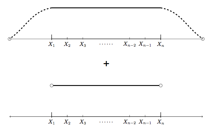
We then use as an estimator of θ\theta, θ^n=arg⁡min​H^p,n​(θ)\widehat{\theta}_{n}=\arg\min\widehat{H}_{p,n}(\theta). An illustration which visualises and compares the boundary corrected Whittle likelihood and hybrid Whittle likelihood is given in Figure 4.
Refer to caption
Refer to caption
Figure 4: Left: The estimated complete DFT and the regular DFT which yields the boundary corrected Whittle likelihood. Right: The estimated complete DFT and the tapered DFT which forms the hybrid Whittle likelihood.

5 The sampling properties of the hybrid Whittle likelihood

In this section, we study the sampling properties of the boundary corrected and hybrid Whittle likelihood. Our focus will be on the hybrid Whittle likelihood as it includes the boundary corrected likelihood as a special case, when ht,n=1h_{t,n}=1 for 1≤t≤n1\leq t\leq n. In Das et al. 2020 we study the sampling properties of the estimated complete periodogram J~n​(ω,f^p)​Jn,h¯n​(ω)¯\widetilde{J}_{n}(\omega;\widehat{f}_{p})\overline{J_{n,\underline{h}_{n}}(\omega)}. Using these results and the results in Appendix D and E, we obtain the bias and variance of the boundary corrected and hybrid Whittle likelihood.

Suppose we fit the spectral density fθ​(ω)f_{\theta}(\omega) (where θ\theta is an unknown dd-dimension parameter vector) to the stationary time series {Xt}t=1n\{X_{t}\}_{t=1}^{n} whose true spectral density is ff. The best fitting spectral density is fθnf_{\theta_{n}}, where θn=arg⁡min​In​(f,fθ)\theta_{n}=\arg\min I_{n}(f;f_{\theta}). Let θ^n=(θ^1,n,…,θ^d,n)\widehat{\theta}_{n}=(\widehat{\theta}_{1,n},\ldots,\widehat{\theta}_{d,n}) be its estimator, where θ^n=arg⁡min​H^p,n​(θ)\widehat{\theta}_{n}=\arg\min\widehat{H}_{p,n}(\theta).

5.1 Assumptions

To derive the sampling properties of θ^n\widehat{\theta}_{n} we assume the data taper has the following form

ht,n=cn​hn​(t/n),\displaystyle h_{t,n}=c_{n}h_{n}(t/n), (5.1)

where hn:[0,1]→ℝh_{n}:[0,1]\rightarrow\mathbb{R} is a sequence of positive functions that satisfy the taper assumptions in Section 5, Dahlhaus 1988 and cn=n/H1,nc_{n}=n/H_{1,n} with Hq,n=∑t=1nhn​(t/n)qH_{q,n}=\sum_{t=1}^{n}h_{n}(t/n)^{q}. We will assume supt,nht,n<∞\sup_{t,n}h_{t,n}<\infty, using this it is straightforward to show H2,n/H1,n2∼n−1H_{2,n}/H_{1,n}^{2}\sim n^{-1}. Under this condition, the hybrid Whittle is n1/2n^{1/2}–consistency and the equivalence result in Theorem 5.1 holds. This assumption is used in Dahlhaus 1983 and in practice one often assumes that a fixed percentage of the data is tapered. A relaxation of the condition H2,n/H1,n2∼n−1H_{2,n}/H_{1,n}^{2}\sim n^{-1} will lead to a change of rate in Theorem 5.1.

Assumption 5.1 (Assumptions on the parameter space)
  • (i)

    The parameter space Θ⊂ℝd\Theta\subset\mathbb{R}^{d} is compact, 0<infθ∈Θinfωfθ​(ω)≤supθ∈Θsupωfθ​(ω)<∞0<\inf_{\theta\in\Theta}\inf_{\omega}f_{\theta}(\omega)\leq\sup_{\theta\in\Theta}\sup_{\omega}f_{\theta}(\omega)<\infty and θn\theta_{n} lies in the interior of Θ\Theta.

  • (ii)

    The one-step ahead prediction error σ2=exp⁡((2​π)−1​∫02​πlog⁡fθ​(ω)​𝑑ω)\sigma^{2}=\exp((2\pi)^{-1}\int_{0}^{2\pi}\log f_{\theta}(\omega)d\omega) is not a function of the parameter θ\theta.

  • (iii)

    Let {ϕj​(fθ)}\{\phi_{j}(f_{\theta})\} and {ψj​(fθ)}\{\psi_{j}(f_{\theta})\} denote the AR(∞)(\infty) and MA(∞)(\infty) coefficients corresponding to the spectral density fθf_{\theta} respectively. Then for all θ∈Θ\theta\in\Theta and 0≤s≤κ0\leq s\leq\kappa (for some κ≥4\kappa\geq 4), we have

    (a)​supθ∈Θ∑j=1∞‖jK​∇θsϕj​(fθ)‖1<∞(b)​supθ∈Θ∑j=1∞‖jK​∇θsψj​(fθ)‖1<∞,(a)\sup_{\theta\in\Theta}\sum_{j=1}^{\infty}\|j^{K}\nabla_{\theta}^{s}\phi_{j}(f_{\theta})\|_{1}<\infty\qquad(b)\sup_{\theta\in\Theta}\sum_{j=1}^{\infty}\|j^{K}\nabla_{\theta}^{s}\psi_{j}(f_{\theta})\|_{1}<\infty,\quad

    where K>3/2K>3/2, ∇θa​g​(fθ)\nabla_{\theta}^{a}g(f_{\theta}) is the aath order partial derivative of gg with respect to θ\theta, and ‖∇θa​g​(fθ)‖1\|\nabla_{\theta}^{a}g(f_{\theta})\|_{1} denotes the absolute sum of all the partial derivatives in ∇θa​g​(fθ)\nabla_{\theta}^{a}g(f_{\theta}).

We use Assumption 5.1(ii, iii) to show that the n−1​∑k=1nlog⁡fθ​(ωk,n)n^{-1}\sum_{k=1}^{n}\log f_{\theta}(\omega_{k,n}) term in boundary corrected and hybrid Whittle likelihoods are negligible with respect the other bias terms. This allows us to simplify some of the bias expansions. Without Assumption 5.1(ii, iii-a) the asymptotic bias of the new-frequency domain likelihood estimators would contain some additional terms. Assumption 5.1(iii-b) is used to bound the ssth derivative of the spectral density.

Assumption 5.2 (Assumptions on the time series)
  • (i)

    {Xt}\{X_{t}\} is a stationary time series. Let κℓ​(t1,…,tℓ−1)\kappa_{\ell}(t_{1},\ldots,t_{\ell-1}) denote the joint cumulant cum⁡(X0,Xt1,…,Xtℓ−1)\mathrm{cum}(X_{0},X_{t_{1}},\ldots,X_{t_{\ell-1}}).

    Then for all 1≤j≤ℓ≤121\leq j\leq\ell\leq 12,

    ∑t1,…,tℓ−1|(1+tj)​κℓ​(t1,…,tℓ−1)|<∞.\displaystyle\sum_{t_{1},\ldots,t_{\ell-1}}|(1+t_{j})\kappa_{\ell}(t_{1},\ldots,t_{\ell-1})|<\infty.
  • (ii)

    The spectral density of {Xt}\{X_{t}\} is such that the spectral density ff is bounded away from zero and for some K>1K>1, the autocovariance function satisfies ∑r∈ℤ|rK​cf​(r)|<∞\sum_{r\in\mathbb{Z}}|r^{K}c_{f}(r)|<\infty.

  • (iii)

    I⁡(θn)I(\theta_{n}) is invertible where

    I(θ)=−12​π∫02​π[∇θ2fθ(ω)−1]f(ω)dω.\displaystyle I(\theta)=-\frac{1}{2\pi}\int_{0}^{2\pi}[\nabla_{\theta}^{2}f_{\theta}(\omega)^{-1}]f(\omega)d\omega. (5.2)

We require Assumption 5.2(i), when ℓ=4\ell=4 and 66 to obtain a bound for the expectation of the terms in the bias expansions and ℓ=12\ell=12 to show equivalence between the feasible estimator based on H^p,n​(θ)\widehat{H}_{p,n}(\theta) and its infeasible counterparts Hn​(θ)H_{n}(\theta). Under Assumption 5.2(i,ii), Theorem 3.1 in Das et al. 2020, we can show that

H^p,n​(θ)=Hn​(θ)+Op​(p3n3/2+1n​pK−1).\displaystyle\widehat{H}_{p,n}(\theta)=H_{n}(\theta)+O_{p}\left(\frac{p^{3}}{n^{3/2}}+\frac{1}{np^{K-1}}\right).

Under Assumption 5.1(i,iii) the above error is uniform over the parameter space. If the model is an AR(p0)(p_{0}) and p0≤pp_{0}\leq p, then the term O⁡((n​pK−1)−1)O((np^{K-1})^{-1}) in the above disappears.

To obtain a bound for the mean and variance of θ^n=(θ^1,n,…,θ^d,n)\widehat{\theta}_{n}=(\widehat{\theta}_{1,n},\ldots,\widehat{\theta}_{d,n}) we require the following quantities. Let

V⁡(g,h)\displaystyle V(g,h) =\displaystyle= 22​π​∫02​πg⁡(ω)​h​(ω)​f​(ω)2​𝑑ω\displaystyle\frac{2}{2\pi}\int_{0}^{2\pi}g(\omega)h(\omega)f(\omega)^{2}d\omega
+1(2​π)2∫02​π∫02​πg(ω1)h(ω2)f4(ω1,−ω1,ω2)dω1dω2\displaystyle+\frac{1}{(2\pi)^{2}}\int_{0}^{2\pi}\int_{0}^{2\pi}g(\omega_{1})h(\omega_{2})f_{4}(\omega_{1},-\omega_{1},\omega_{2})d\omega_{1}d\omega_{2}
andJ⁡(g)\displaystyle\text{and}\qquad\qquad J(g) =\displaystyle= 12​π​∫02​πg⁡(ω)​f​(ω)​𝑑ω,\displaystyle\frac{1}{2\pi}\int_{0}^{2\pi}g(\omega)f(\omega)d\omega, (5.3)

where f4f_{4} denotes the fourth order cumulant density of the time series {Xt}\{X_{t}\}. We denote the (s,r)(s,r)th element of I​(θn)−1I(\theta_{n})^{-1} (where I⁡(θn)I(\theta_{n}) is defined in (5.2)) as I(s,r)I^{(s,r)}, and define

Gr​(θ)\displaystyle G_{r}(\theta) =\displaystyle= ∑s1,s2=1dI(s1,s2)​V​(∂fθ−1∂θs2,∂2fθ−1∂θs1​∂θr)\displaystyle\sum_{s_{1},s_{2}=1}^{d}I^{(s_{1},s_{2})}V\left(\frac{\partial f_{\theta}^{-1}}{\partial\theta_{s_{2}}},\frac{\partial^{2}f_{\theta}^{-1}}{\partial\theta_{s_{1}}\partial\theta_{r}}\right) (5.4)
+12∑s1,s2,s3,s4=1dI(s1,s3)I(s2,s4)V(∂fθ−1∂θs3,∂fθ−1∂θs4)J(∂3fθ−1∂θs1​∂θs2​∂θr).\displaystyle+\frac{1}{2}\sum_{s_{1},s_{2},s_{3},s_{4}=1}^{d}I^{(s_{1},s_{3})}I^{(s_{2},s_{4})}V\left(\frac{\partial f_{\theta}^{-1}}{\partial\theta_{s_{3}}},\frac{\partial f_{\theta}^{-1}}{\partial\theta_{s_{4}}}\right)J\left(\frac{\partial^{3}f_{\theta}^{-1}}{\partial\theta_{s_{1}}\partial\theta_{s_{2}}\partial\theta_{r}}\right).

5.2 The asymptotic sampling properties

Using the assumptions above we obtain a bound between the feasible and infeasible estimators.

Theorem 5.1 (Equivalence of feasible and infeasible estimators)

Suppose Assumptions 5.1 and 5.2 hold. Define the feasible and infeasible estimators as θ~n=arg⁡min​Hn​(θ)\widetilde{\theta}_{n}=\arg\min H_{n}(\theta) and θ^n=arg⁡min​H^p,n​(θ)\widehat{\theta}_{n}=\arg\min\widehat{H}_{p,n}(\theta) respectively. Then for p≥1p\geq 1 we have

|θ^n−θ~n|1=Op​(p3n3/2+1n​pK−1),\displaystyle|\widehat{\theta}_{n}-\widetilde{\theta}_{n}|_{1}=O_{p}\left(\frac{p^{3}}{n^{3/2}}+\frac{1}{np^{K-1}}\right),

where |a|1=∑j=1d|aj||a|_{1}=\sum_{j=1}^{d}|a_{j}|. For the case p=0p=0, θ^n\widehat{\theta}_{n} is the parameter estimator based on the Whittle likelihood using the one-sided tapered periodogram Jn​(ωk,n)​Jn,h¯n​(ωk,n)¯J_{n}(\omega_{k,n})\overline{J_{n,\underline{h}_{n}}(\omega_{k,n})} rather than the regular tapered periodogram. In this case, |θ^n−θ~n|1=Op​(n−1)|\widehat{\theta}_{n}-\widetilde{\theta}_{n}|_{1}=O_{p}\left(n^{-1}\right).

Note if the true spectral density of the time series is that of an AR(p0)(p_{0}) where p0≤pp_{0}\leq p, then the O⁡((n​pK−1)−1)O((np^{K-1})^{-1}) term is zero.

PROOF. In Appendix D. □\Box

The implication of the equivalence result is if p3/n1/2→0p^{3}/n^{1/2}\rightarrow 0 as p→∞p\rightarrow\infty and n→∞n\rightarrow\infty, then n​|θ^n−θ~n|1→0n|\widehat{\theta}_{n}-\widetilde{\theta}_{n}|_{1}\rightarrow 0 and asymptotically the properties of the infeasible estimator (such as bias and variance) transfer to the feasible estimator.

5.2.1 The bias and variance of the hybrid Whittle likelihood

The expressions in this section are derived under Assumptions 5.1 and 5.2.

The bias We show in Appendix E.4, that the asymptotic bias (in the sense of Bartlett) for θ^n=(θ^1,n,…,θ^d,n)\widehat{\theta}_{n}=(\widehat{\theta}_{1,n},\ldots,\widehat{\theta}_{d,n}) is

𝔼⁡[θ^j,n−θj,n]=H2,nH1,n2​∑r=1dI(j,r)​Gr​(θn)+O⁡(p3n3/2+1n​pK−1)1≤j≤d,\displaystyle\mathbb{E}[\widehat{\theta}_{j,n}-\theta_{j,n}]=\frac{H_{2,n}}{H_{1,n}^{2}}\sum_{r=1}^{d}I^{(j,r)}G_{r}(\theta_{n})+O\left(\frac{p^{3}}{n^{3/2}}+\frac{1}{np^{K-1}}\right)\quad 1\leq j\leq d, (5.5)

where I(j,r)I^{(j,r)} and Gr​(θn)G_{r}(\theta_{n}) is defined in (5.4). We note that if no tapering were used then H2,n/H1,n2=n−1H_{2,n}/H_{1,n}^{2}=n^{-1}. The Gaussian and Whittle likelihood have a bias which includes the above term (where H2,n/H1,n2=n−1H_{2,n}/H_{1,n}^{2}=n^{-1}) plus an additional term of the form ∑r=1dI(j,r)​𝔼​[∇θLn​(θn)]\sum_{r=1}^{d}I^{(j,r)}\mathbb{E}[\nabla_{\theta}L_{n}(\theta_{n})], where Ln​(⋅)L_{n}(\cdot) is the Gaussian or Whittle likelihood (see Appendix E.4 for the details).

Theoretically, it is unclear which criteria has the smallest bias (since the inclusion of additional terms does not necessarily increase the bias). However, for the hybrid Whittle likelihood estimator, a straightfoward “Bartlett correction” can be made to estimate the bias in (5.5). We briefly outline how this can be done. We observe that the bias is built of I⁡(⋅)I(\cdot), J⁡(⋅)J(\cdot) and V⁡(⋅,⋅)V(\cdot,\cdot). Both I⁡(⋅)I(\cdot) and J⁡(⋅)J(\cdot) can easily be estimated with their sample means. The term V⁡(⋅,⋅)V(\cdot,\cdot) can also be estimated by using an adaption of orthogonal samples (see Subba Rao 2018), which we now describe. Define the random variable

hr​(g,f)=1n​∑k=1ng⁡(ωk,n)​J~n​(ωk+r,n,f)​Jn​(ωk,n)¯forr≥1,\displaystyle h_{r}(g;f)=\frac{1}{n}\sum_{k=1}^{n}g(\omega_{k,n})\widetilde{J}_{n}(\omega_{k+r,n};f)\overline{J_{n}(\omega_{k,n})}\quad\textrm{for}\quad r\geq 1,

where gg is a continuous and bounded function. Suppose g1g_{1} and g2g_{2} are continuous and bounded functions. If r≠n​ℤr\neq n\mathbb{Z}, then 𝔼f​[hr​(gj,f)]=0\mathbb{E}_{f}[h_{r}(g_{j};f)]=0 (for j=1j=1 and 22). But interestingly, if r<<nr<<n, then n​covf​[hr​(g1,f),hr​(g2,f)]=n​𝔼f​[hr​(g1,f)​hr​(g2,f)¯]=V⁡(g1,g2)+O⁡(r/n)n\mathrm{cov}_{f}[h_{r}(g_{1};f),h_{r}(g_{2};f)]=n\mathbb{E}_{f}[h_{r}(g_{1};f)\overline{h_{r}(g_{2};f)}]=V(g_{1},g_{2})+O(r/n). Using these results, we estimate V⁡(g1,g2)V(g_{1},g_{2}) by replacing hr​(gj,f)h_{r}(g_{j};f) with hr​(gj,f^p)h_{r}(g_{j};\widehat{f}_{p}) and defining the “sample covariance”

V^M​(g1,g2)=nM​∑r=1Mhr​(g1,f^p)​hr​(g2,f^p)¯\displaystyle\widehat{V}_{M}(g_{1},g_{2})=\frac{n}{M}\sum_{r=1}^{M}h_{r}(g_{1};\widehat{f}_{p})\overline{h_{r}(g_{2};\widehat{f}_{p})}

where M<<nM<<n. Thus, V^M​(g1,g2)\widehat{V}_{M}(g_{1},g_{2}) is an estimator of V⁡(g1,g2)V(g_{1},g_{2}). Based on this construction,

V^M​(∂∂θs2​fθ^n−1,∂2∂θs1​∂θr​fθ^n−1)andV^M​(∂∂θs3​fθ^n−1,∂∂θs4​fθ^n−1)\displaystyle\widehat{V}_{M}\left(\frac{\partial}{\partial\theta_{s_{2}}}f_{\widehat{\theta}_{n}}^{-1},\frac{\partial^{2}}{\partial\theta_{s_{1}}\partial\theta_{r}}f_{\widehat{\theta}_{n}}^{-1}\right)\quad\textrm{and}\quad\widehat{V}_{M}\left(\frac{\partial}{\partial\theta_{s_{3}}}f_{\widehat{\theta}_{n}}^{-1},\frac{\partial}{\partial\theta_{s_{4}}}f_{\widehat{\theta}_{n}}^{-1}\right)

are estimators of V⁡(∂fθ−1∂θs2,∂2fθ−1∂θs1​∂θr)V\left(\frac{\partial f_{\theta}^{-1}}{\partial\theta_{s_{2}}},\frac{\partial^{2}f_{\theta}^{-1}}{\partial\theta_{s_{1}}\partial\theta_{r}}\right) and V⁡(∂fθ−1∂θs3,∂fθ−1∂θs4)V\left(\frac{\partial f_{\theta}^{-1}}{\partial\theta_{s_{3}}},\frac{\partial f_{\theta}^{-1}}{\partial\theta_{s_{4}}}\right) respectively. This estimation scheme yields a consistent estimate of the bias even when the model is misspecified. In contrast, it is unclear how a bias correction would work for the Gaussian and Whittle likelihood under misspecification, as they also involve the term 𝔼f​[∇θLn​(θn)]\mathbb{E}_{f}[\nabla_{\theta}L_{n}(\theta_{n})]. In the case of misspecification, 𝔼f​[∇θLn​(θn)]≠0\mathbb{E}_{f}[\nabla_{\theta}L_{n}(\theta_{n})]\neq 0 and is of order O⁡(n−1)O(n^{-1}).

It is worth mentioning that the asymptotic expansion in (5.5) does not fully depict what we observe in the simulations in Section 6. A theoretical comparison of the biases of both new likelihoods show that for the boundary corrected Whittle likelihood, the bias is asymptotically n−1​∑r=1dI(j,r)​Gr​(θn)n^{-1}\sum_{r=1}^{d}I^{(j,r)}G_{r}(\theta_{n}), whereas when tapering is used the bias is (H2,n/H1,n2)​∑r=1dI(j,r)​Gr​(θn)≥n−1​∑r=1dI(j,r)​Gr​(θn)(H_{2,n}/H_{1,n}^{2})\sum_{r=1}^{d}I^{(j,r)}G_{r}(\theta_{n})\geq n^{-1}\sum_{r=1}^{d}I^{(j,r)}G_{r}(\theta_{n}). This would suggest that the hybrid Whittle likelihood should have a larger bias than the boundary corrected Whittle likelihood. But the simulations (see Section 6) suggest this is not necessarily true and the hybrid likelihood tends to have a smaller bias.

The variance We show in Corollary 3.1, Das et al. 2020 that the inclusion of the prediction DFT in the hybrid Whittle likelihood has a variance which asymptotically is small as compared with the main Whittle term if p3/n→0p^{3}/n\rightarrow 0 as p,n→∞p,n\rightarrow\infty (under the condition H2,n/H1,n2∼n−1H_{2,n}/H_{1,n}^{2}\sim n^{-1}) Using this observation, standard Taylor expansion methods and Corollary 3.1 in Das et al. 2020, the asymptotic variance of θ^n\widehat{\theta}_{n} is

H1,n2H2,nvar(θ^n)=I(θn)−1V(∇θfθ−1,∇θfθ−1)⌋θ=θnI(θn)−1+o(1),\displaystyle\frac{H_{1,n}^{2}}{H_{2,n}}\mathrm{var}(\widehat{\theta}_{n})=I(\theta_{n})^{-1}V\left(\nabla_{\theta}f_{\theta}^{-1},\nabla_{\theta}f_{\theta}^{-1}\right)\rfloor_{\theta=\theta_{n}}I(\theta_{n})^{-1}+o(1),

where V⁡(⋅)V(\cdot) is defined in (5.3).

5.2.2 The role of order estimation on the rates

The order in the AR(p)(p) approximation is selected using the AIC, where p^=arg⁡min​AIC​(p)\widehat{p}=\arg\min\text{AIC}(p) with

AIC​(p)=log⁡σ^p,n2+2​pn,\displaystyle\text{AIC}(p)=\log\widehat{\sigma}_{p,n}^{2}+\frac{2p}{n},

σ^p,n2=1n−Kn​∑t=Knn(Xt−∑j=1pϕ^j,p​Xt−j)2\widehat{\sigma}_{p,n}^{2}=\frac{1}{n-K_{n}}\sum_{t=K_{n}}^{n}(X_{t}-\sum_{j=1}^{p}\widehat{\phi}_{j,p}X_{t-j})^{2}, KnK_{n} is such that Kn2+δ∼nK_{n}^{2+\delta}\sim n for some δ>0\delta>0. Ing and Wei 2005 assume that the underlying time series is a linear, stationary time series with an AR(∞)(\infty) that satisfies Assumption K.1−-K.4 in Ing and Wei 2005. They show that under the condition that the AR(∞)(\infty) coefficients satisfy (∑j=p+1∞|ϕj|)2=O⁡(p−2​K)(\sum_{j=p+1}^{\infty}|\phi_{j}|)^{2}=O(p^{-2K}), then p^=Op​(n1/(1+2​K))\widehat{p}=O_{p}(n^{1/(1+2K)}) (see Example 2 in Ing and Wei 2005). Thus, if K>5/2K>5/2, then p^3/n1/2→𝒫0\widehat{p}^{3}/n^{1/2}\stackrel{{\scriptstyle\mathcal{P}}}{{\rightarrow}}0 (where p^=Op​(n1/(1+2​K))\widehat{p}=O_{p}(n^{1/(1+2K)})) and p^→𝒫∞\widehat{p}\stackrel{{\scriptstyle\mathcal{P}}}{{\rightarrow}}\infty as n→∞n\rightarrow\infty. These rates ensure that the difference between the feasible and infeasible estimator is |θ^n−θ~n|1=op​(n−1)|\widehat{\theta}_{n}-\widetilde{\theta}_{n}|_{1}=o_{p}(n^{-1}). Thus the feasible estimator, constructed using the AIC, and the infeasible estimator are equivalent and the bias and variance derived above are valid for this infeasible estimator.

5.2.3 The computational cost of the estimators

We now discuss some of the implementation issues of the new estimators.

The Durbin-Levinson algorithm is often used to maximize the Gaussian likelihood. If this is employed, then the computational cost of the algorithm is O⁡(n2)O(n^{2}). On the other hand, by using the FFT, the computational cost of the Whittle likelihood is O⁡(n​log⁡n)O(n\log n).

For the boundary corrected Whittle and hybrid Whittle likelihood algorithm, there is an additional cost over the Whittle likelihood due to the estimation of {J^n​(ωk,n,f^p)}k=1n\{\widehat{J}_{n}(\omega_{k,n};\widehat{f}_{p})\}_{k=1}^{n}. We recall that f^p\widehat{f}_{p} is constructed using the Yule-Walker estimator ϕ¯^p=(ϕ^1,p,…,ϕ^p,p)′\widehat{\underline{\phi}}_{p}=(\widehat{\phi}_{1,p},...,\widehat{\phi}_{p,p})^{\prime} where pp is selected with the AIC. We now calculate the complexity of calculating {J^n​(ωk,n,f^p)}k=1n\{\widehat{J}_{n}(\omega_{k,n};\widehat{f}_{p})\}_{k=1}^{n}.

The sample autocovariances, {c^n​(r)}r=0n−1\{\widehat{c}_{n}(r)\}_{r=0}^{n-1} (which are required in the Yule-Walker estimator) can be calculated in O⁡(n​log⁡n)O(n\log n) operations. Let KnK_{n} denote the maximum order used for the evaluation of the AIC. If we implement the Durbin-Levinson algorithm, then evaluating ϕ¯^p\widehat{\underline{\phi}}_{p} for 1≤p≤Kn1\leq p\leq K_{n} requires in total O⁡(Kn2)O(K_{n}^{2}) arithmetic operations. Given the estimated AR coefficients ϕ¯^p^\widehat{\underline{\phi}}_{\hat{p}}, the predictive DFT {J^n​(ωk,n,f^p)}k=1n\{\widehat{J}_{n}(\omega_{k,n};\widehat{f}_{p})\}_{k=1}^{n} can be calculated in O⁡(min⁡(n​log⁡n,n​p^))O(\min(n\log n,n\hat{p})) arithmetic operations (the details of the algorithm for optimal calculation can be found in Appendix A.1). Therefore, the overall computational cost of implementing both the boundary corrected Whittle and hybrid Whittle likelihood algorithms is O⁡(n​log⁡n+Kn2)O(n\log n+K_{n}^{2}).

Using Ing and Wei 2005 Example 2, for consistent order selection KnK_{n} should be such that Kn∼n1/(2​K+1)+εK_{n}\sim n^{1/(2K+1)+\varepsilon} for some ε>0\varepsilon>0 (where KK is defined in Assumption 3.1). Therefore, we conclude that the computational cost of the new likelihoods is of the same order as the Whittle likelihood.

6 Empirical results

To substantiate our theoretical results, we conduct some simulations (further simulations can be found in Appendix F, G and H). To compare different methods, we evaluate six different quasi-likelihoods: the Gaussian likelihood (equation (1.1)), the Whittle likelihood (equation (1.3)), the boundary corrected Whittle likelihood (equation (4.8)), the hybrid Whittle likelihood (equation (4.11)), the tapered Whittle likelihood (p.810 of Dahlhaus 1988) and the debiased Whittle likelihood (equation (7) in Sykulski et al. 2019).

The tapered and hybrid Whittle likelihoods require the use of data tapers. We use a Tukey taper (also known as the cosine-bell taper) where

hn​(t/n)={12​[1−cos⁡(π⁡(t−12)/d)]1≤t≤d1d+1≤t≤n−d12​[1−cos⁡(π⁡(n−t+12)/d)]n−d+1≤t≤n.\displaystyle h_{n}\left(t/n\right)=\left\{\begin{array}[]{ll}\frac{1}{2}[1-\cos(\pi(t-\frac{1}{2})/d)]&1\leq t\leq d\\ 1&d+1\leq t\leq n-d\\ \frac{1}{2}[1-\cos(\pi(n-t+\frac{1}{2})/d)]&n-d+1\leq t\leq n\end{array}.\right.

We set the proportion of tapering at each end of the time series is 0.10.1, i.e. d=n/10d=n/10 (the default in R).

When evaluating the boundary corrected Whittle likelihood and hybrid Whittle likelihood, the order pp is selected with the AIC and f^p\widehat{f}_{p} is estimated using the Yule-Walker estimator.

Unlike the Whittle, the tapered Whittle and debiased Whittle likelihood, Re⁡J~n​(ωk,n,f^p)​Jn​(ωk,n)¯\operatorname{Re}\widetilde{J}_{n}(\omega_{k,n};\widehat{f}_{p})\overline{J_{n}(\omega_{k,n})} and Re⁡J~n​(ωk,n,f^p)​Jn,h¯n​(ωk,n)¯\operatorname{Re}\widetilde{J}_{n}(\omega_{k,n};\widehat{f}_{p})\overline{J_{n,\underline{h}_{n}}(\omega_{k,n})} can be negative. To avoid negative values, we apply the thresholding function f⁡(t)=max⁡(t,10−3)f(t)=\max(t,10^{-3}) to Re⁡J~n​(ωk,n,f^p)​Jn​(ωk,n)¯\operatorname{Re}\widetilde{J}_{n}(\omega_{k,n};\widehat{f}_{p})\overline{J_{n}(\omega_{k,n})} and Re⁡J~n​(ωk,n,f^p)​Jn,h¯n​(ωk,n)¯\operatorname{Re}\widetilde{J}_{n}(\omega_{k,n};\widehat{f}_{p})\overline{J_{n,\underline{h}_{n}}(\omega_{k,n})} over all the frequencies. Thresholding induces an additional (small) bias to the new criteria. The proportion of times that Re⁡J~n​(ωk,n,f^p)​Jn​(ωk,n)¯\operatorname{Re}\widetilde{J}_{n}(\omega_{k,n};\widehat{f}_{p})\overline{J_{n}(\omega_{k,n})} drops below the threshold increases for spectral density functions with large peaks and when the spectral density is close to zero. However, at least for the models that we studied in the simulations, the bias due to the thresholding is negligible.

All simulations are conducted over 1000 replications with sample sizes n=20n=20, 5050, and 300300. In all the tables below and Appendix, the bias of the estimates are in parenthesis and the standard deviation are in parenthesis. The ordering of the performance of the estimators is colour coded and is based on their squared root of the mean squared error (RMSE).

6.1 Estimation with correctly specified models

We first study the AR(1) and MA(1) parameter estimates when the models are correctly specified. We generate two types of time series models X¯n\underline{X}_{n} and Y¯n\underline{Y}_{n}, which satisfy the following recursions

𝐀𝐑⁡(𝟏):\displaystyle{\bf AR(1)}: Xt=θ​Xt−1+et;ϕX​(ω)=1−θ​e−i​ω\displaystyle X_{t}=\theta X_{t-1}+e_{t};\quad\phi_{X}(\omega)=1-\theta e^{-i\omega}
𝐌𝐀⁡(𝟏):\displaystyle{\bf MA(1)}: Yt=et+θ​et−1;ϕY​(ω)=(1+θ​e−i​ω)−1,\displaystyle Y_{t}=e_{t}+\theta e_{t-1};\quad\phi_{Y}(\omega)=(1+\theta e^{-i\omega})^{-1},

where |θ|<1|\theta|<1, {et}\{e_{t}\} are independent, identically distributed Gaussian random variables with mean 0 and variance 1. Note that the Gaussianity of the innovations is not required to obtain the theoretical properties of the estimations. In Appendix F.2, we include simulations when the innovations follow a standardized chi-squared distribution with two degrees of freedom. The results are similar to those with Gaussian innovations. We generate the AR(1)(1) and MA(1)(1) models with parameters θ=0.1,0.3,0.5,0.7\theta=0.1,0.3,0.5,0.7 and 0.90.9. For the time series generated by an AR(1)(1) process, we fit an AR(1)(1) model, similarly, for the time series generated by a MA(1)(1) process we fit a MA(1)(1) model.

For each simulation, we evaluate the six different parameter estimators. The empirical bias and standard deviation are calculated. Figures 5 gives the bias (first row) and the RMSE (second row) of each estimated parameter θ\theta for both AR(1)(1) and MA(1)(1) models. We focus on positive θ\theta, similar results are obtained for negative θ\theta. The results are also summarized in Table 3 in Appendix F.1.

AR(1)(1) model

MA(1)(1) model

Figure 5: Bias (first row) and the RMSE (second row) of the parameter estimates for the Gaussian AR(1) models and Gaussian MA(1) models. Length of the time series n=20n=20(left), 5050(middle), and 300300(right).

For both AR(1)(1) and MA(1)(1) models, we observe a stark difference between the bias of the Whittle likelihood estimator (blue line) and the other five other methods, which in most cases have a lower bias. The Gaussian likelihood performs uniformly well for both models and all sample sizes. Whereas, the tapered Whittle estimator performs very well for the MA(1)(1) model but not quite as well for the AR(1)(1) model. The debiased Whittle likelihood performs quite well for both models, especially when the parameter values are small (e.g. θ=0.1,0.3\theta=0.1,0.3, and 0.50.5).

The simulations suggest that the boundary corrected and hybrid Whittle likelihoods (referred from now on as the new likelihoods) are competitive with the benchmark Gaussian likelihood for both AR(1)(1) and MA(1)(1) models. For the AR(1)(1) model the new likelihoods tend to have the smallest or second smallest RMSE (over all sample sizes and more so when ϕ\phi is large). A caveat is that for the AR(1)(1) model the bias of the boundary corrected and hybrid Whittle tends to be a little larger than the bias of the Gaussian likelihood (especially for the smaller sample sizes). This is interesting, because in Appendix E.2 we show that if the AR(1)(1) model is correctly specified, the first order bias of the boundary corrected Whittle likelihood and the Gaussian likelihood are the same (both are −2θ/n-2\theta/n). The bias of the hybrid Whittle likelihood is slightly large, due to the data taper. However, there are differences in the second order expansions. Specifically, for the Gaussian likelihood, it is O(n−3/2)O(n^{-3/2}), whereas, for the boundary corrected and hybrid Whittle it is O(p3n−3/2)O(p^{3}n^{-3/2}). Indeed, the O(p3n−3/2)O(p^{3}n^{-3/2}) term arises because of the parameter estimation in the predictive DFT. This term is likely to dominate the O(n−3/2)O(n^{-3/2}) in the Gaussian likelihood. Therefore, for small sample sizes, the second order terms can impact the bias. It is this second order term that may be causing the larger bias seen in the boundary corrected Whittle likelihood as compared with the Gaussian likelihood.

On the other hand, the bias for the MA(1)(1) model tends to be smaller for the new likelihoods, including the benchmark Gaussian likelihood. Surprisingly, there appears to be examples where the new likelihood does better (in terms of RMSE) than the Gaussian likelihood. This happens when n∈{50,300}n\in\{50,300\} for θ=0.9\theta=0.9. This observation is noteworthy, as the computational cost of the Gaussian likelihood is greater than the computational cost of the new likelihoods (see Section 5.2). Thus the simulations suggest that in certain situations the new estimator may outperform the Gaussian likelihood at a lower computational cost.

In summary, the new likelihoods perform well compared with the standard methods, including the benchmark Gaussian likelihood. As expected, for large sample sizes the performance of all the estimators improves considerably. And for some models, the new likelihood is able to outperform the Gaussian likelihood estimator. Though there is no clear rule when this will happen.

6.2 Estimation under misspecification

Next, we turn into our attention to the case that the model is misspecified (which is more realistic for real data). As we mentioned above, the estimation of the AR parameters in the predictive DFT of the new likelihoods leads to an additional error of order O(p3n−3/2)O(p^{3}n^{-3/2}). The more complex the model, the larger pp will be, leading to a larger O(p3n−3/2)O(p^{3}n^{-3/2}). To understand the effect this may have for small sample sizes, in this section we fit a simple model to a relatively complex process.

For the “true” data generating process we use an ARMA(3,2)(3,2) Gaussian time series with spectral density fZ​(ω)=|ψZ​(e−i​ω)|2/|ϕZ​(e−i​ω)|2f_{Z}(\omega)=|\psi_{Z}(e^{-i\omega})|^{2}/|\phi_{Z}(e^{-i\omega})|^{2}, where AR and MA characteristic polynomials are

ϕZ​(z)=(1−0.7​z)​(1−0.9​ei​z)​(1−0.9​e−i​z)andψZ​(z)=(1+0.5​z+0.5​z2).\phi_{Z}(z)=(1-0.7z)(1-0.9e^{i}z)(1-0.9e^{-i}z)\quad{\textrm{and}}\quad\psi_{Z}(z)=(1+0.5z+0.5z^{2}).

This spectral density has some interesting characteristics: a pronounced peak, a large amount of power at the low frequencies, and a sudden drop in power at the higher frequencies. We consider sample sizes n=20,50n=20,50 and 300300, and fit a model with fewer parameters. Specifically, we fit two different ARMA models with the same number of unknown parameters. The first is the ARMA(1,1) model with spectral density

fθ​(ω)=|1+ψ​e−i​ω|2​|1−ϕ​e−i​ω|−2θ=(ϕ,ψ).f_{\theta}(\omega)=|1+\psi e^{-i\omega}|^{2}|1-\phi e^{-i\omega}|^{-2}\qquad\theta=(\phi,\psi).

The second is the AR(2) model with spectral density

fθ​(ω)=|1−ϕ1​e−i​ω−ϕ2​e−2​i​ω|−2θ=(ϕ1,ϕ2).f_{\theta}(\omega)=|1-\phi_{1}e^{-i\omega}-\phi_{2}e^{-2i\omega}|^{-2}\qquad\theta=(\phi_{1},\phi_{2}).

Figure 6 shows the logarithm of the theoretical ARMA(3,2) spectral density (solid line, fZf_{Z}) and the corresponding log spectral densities of the best fitting ARMA(1,1) (dashed line) and AR(2) (dotted line) processes for n=20n=20. The best fitting models are obtained by minimizing the spectral divergence θB​e​s​t=arg⁡minθ∈Θ​In​(f,fθ)\theta^{Best}=\arg\min_{\theta\in\Theta}I_{n}(f;f_{\theta}), where In​(f,fθ)I_{n}(f,f_{\theta}) is defined in (4.1) and Θ\Theta is the parameter space. The best fitting models for n=50n=50 and 300300 are similar. We observe that neither of the misspecified models capture all of the features of the true spectral density. The best fitting ARMA(1,1) model has a large amount of power at the low frequencies and the power declines for the higher frequencies. The best fitting AR(2) model peaks around frequency 0.8, but the power at the low frequencies is small. Overall, the spectral divergence between the true and the best fitting AR(2) model is smaller than the spectral divergence between the true and the best ARMA(1,1) model.

Figure 6: Plot of log⁡fZ​(ω)\log f_{Z}(\omega) and log⁡fθB​e​s​t​(ω)\log f_{\theta^{Best}}(\omega); Theoretical ARMA(3,2) spectral density (solid), best fitting ARMA(1,1) spectral density (dashed), and best fitting AR(2) spectral density (dotted) for n=20n=20.

For each simulation, we calculate the six different parameter estimators and the spectral divergence. The result of the estimators using the six different quasi-likelihoods is given in Table 1 (for ARMA(1,1)) and Table 2 (for AR(2)).

nn Parameter Gaussian Whittle Boundary Hybrid Tapered Debiased
20 ϕ\phi 0.031​(0.1)0.031(0.1) -0.095​(0.16)0.095(0.16) -0.023​(0.12)0.023(0.12) -0.006​(0.1)0.006(0.1) -0.080​(0.13)0.080(0.13) 0.187​(0.11)0.187(0.11)
ψ\psi 0.069​(0.08)0.069(0.08) -0.172​(0.18)0.172(0.18) -0.026​(0.14)0.026(0.14) 0.028​(0.1)0.028(0.1) -0.068​(0.12)0.068(0.12) 0.093​(0.06)0.093(0.06)
In​(f,fθ)I_{n}(f;f_{\theta}) 1.653​(0.81)1.653(0.81) 1.199​(1.57)1.199(1.57) 0.945​(0.84)0.945(0.84) 1.024​(0.89)1.024(0.89) 0.644​(0.61)0.644(0.61) 2.727​(0.73)2.727(0.73)
50 ϕ\phi 0.012​(0.07)0.012(0.07) -0.054​(0.09)0.054(0.09) -0.006​(0.07)0.006(0.07) 0.004​(0.07)0.004(0.07) -0.005​(0.07)0.005(0.07) 0.154​(0.11)0.154(0.11)
ψ\psi 0.029​(0.06)0.029(0.06) -0.116​(0.12)0.116(0.12) -0.008​(0.08)0.008(0.08) 0.009​(0.07)0.009(0.07) 0.011​(0.06)0.011(0.06) 0.093​(0)0.093(0)
In​(f,fθ)I_{n}(f;f_{\theta}) 0.354​(0.34)0.354(0.34) 0.457​(0.46)0.457(0.46) 0.292​(0.3)0.292(0.3) 0.235​(0.28)0.235(0.28) 0.225​(0.26)0.225(0.26) 1.202​(0.34)1.202(0.34)
300 ϕ\phi 0.002​(0.03)0.002(0.03) -0.014​(0.03)0.014(0.03) 0​(0.03)0(0.03) 0.001​(0.03)0.001(0.03) 0​(0.03)0(0.03) 0.093​(0.08)0.093(0.08)
ψ\psi 0.005​(0.03)0.005(0.03) -0.033​(0.05)0.033(0.05) 0.001​(0.03)0.001(0.03) 0.003​(0.03)0.003(0.03) 0.003​(0.03)0.003(0.03) 0.092​(0.01)0.092(0.01)
In​(f,fθ)I_{n}(f;f_{\theta}) 0.027​(0.05)0.027(0.05) 0.064​(0.09)0.064(0.09) 0.029​(0.05)0.029(0.05) 0.026​(0.04)0.026(0.04) 0.027​(0.05)0.027(0.05) 0.752​(0.22)0.752(0.22)
Best fitting ARMA(1,1)(1,1) coefficients θ=(ϕ,ψ)\theta=(\phi,\psi) and spectral divergence:
−- θ20=(0.693,0.845)\theta_{20}=(0.693,0.845), θ50=(0.694,0.857)\theta_{50}=(0.694,0.857), θ300=(0.696,0.857)\theta_{300}=(0.696,0.857).
−- I20​(f,fθ)=3.773I_{20}(f;f_{\theta})=3.773, I50​(f,fθ)=3.415I_{50}(f;f_{\theta})=3.415, I300​(f,fθ)=3.388I_{300}(f;f_{\theta})=3.388.
Table 1: The bias of estimated coefficients for six different estimation methods for the Gaussian ARMA(3,2)(3,2) misspecified case fitting ARMA(1,1)(1,1) model. Standard deviations are in the parentheses. We use red to denote the smallest RMSE and blue to denote the second smallest RMSE.
nn Parameter Gaussian Whittle Boundary Hybrid Tapered Debiased
20 ϕ1\phi_{1} 0.028​(0.14)0.028(0.14) -0.162​(0.22)0.162(0.22) -0.032​(0.16)0.032(0.16) 0.003​(0.14)0.003(0.14) -0.123​(0.16)0.123(0.16) 0.069​(0.15)0.069(0.15)
ϕ2\phi_{2} -0.004​(0.09)0.004(0.09) 0.169​(0.18)0.169(0.18) 0.052​(0.14)0.052(0.14) 0.025​(0.12)0.025(0.12) 0.132​(0.12)0.132(0.12) -0.034​(0.11)0.034(0.11)
In​(f,fθ)I_{n}(f;f_{\theta}) 0.679​(0.72)0.679(0.72) 1.203​(1.46)1.203(1.46) 0.751​(0.85)0.751(0.85) 0.684​(0.8)0.684(0.8) 0.862​(0.97)0.862(0.97) 0.686​(0.81)0.686(0.81)
50 ϕ1\phi_{1} 0.019​(0.09)0.019(0.09) -0.077​(0.12)0.077(0.12) -0.009​(0.09)0.009(0.09) 0.003​(0.09)0.003(0.09) -0.017​(0.09)0.017(0.09) 0.156​(0.15)0.156(0.15)
ϕ2\phi_{2} -0.024​(0.06)0.024(0.06) 0.066​(0.1)0.066(0.1) 0.006​(0.07)0.006(0.07) -0.003​(0.06)0.003(0.06) 0.013​(0.06)0.013(0.06) -0.121​(0.06)0.121(0.06)
In​(f,fθ)I_{n}(f;f_{\theta}) 0.275​(0.33)0.275(0.33) 0.382​(0.45)0.382(0.45) 0.283​(0.37)0.283(0.37) 0.283​(0.37)0.283(0.37) 0.283​(0.36)0.283(0.36) 0.65​(0.7)0.65(0.7)
300 ϕ1\phi_{1} 0.004​(0.04)0.004(0.04) -0.013​(0.04)0.013(0.04) 0​(0.04)0(0.04) 0.001​(0.04)0.001(0.04) 0.001​(0.04)0.001(0.04) 0.014​(0.04)0.014(0.04)
ϕ2\phi_{2} -0.005​(0.02)0.005(0.02) 0.011​(0.03)0.011(0.03) -0.001​(0.02)0.001(0.02) -0.001​(0.03)0.001(0.03) -0.001​(0.03)0.001(0.03) 0.016​(0.04)0.016(0.04)
In​(f,fθ)I_{n}(f;f_{\theta}) 0.049​(0.07)0.049(0.07) 0.053​(0.07)0.053(0.07) 0.049​(0.07)0.049(0.07) 0.053​(0.07)0.053(0.07) 0.054​(0.08)0.054(0.08) 0.058​(0.08)0.058(0.08)
Best fitting AR(1)(1) coefficients θ=(ϕ1,ϕ2)\theta=(\phi_{1},\phi_{2}) and spectral divergence:
−- θ20=(1.367,−0.841)\theta_{20}=(1.367,-0.841), θ50=(1.364,−0.803)\theta_{50}=(1.364,-0.803), θ300=(1.365,−0.802)\theta_{300}=(1.365,-0.802).
−- I20​(f,fθ)=2.902I_{20}(f;f_{\theta})=2.902, I50​(f,fθ)=2.937I_{50}(f;f_{\theta})=2.937, I300​(f,fθ)=2.916I_{300}(f;f_{\theta})=2.916.
Table 2: Same as in Table 1 but fitting AR(2) model.

We first discuss the parameter estimates. Comparing the asymptotic bias of the Gaussian likelihood with the boundary corrected Whittle likelihood (see Appendix E.4), the Gaussian likelihood has an additional bias term of form ∑r=1dI(j,r)𝔼[∂ℒn∂θr]⌋θn\sum_{r=1}^{d}I^{(j,r)}\mathbb{E}[\frac{\partial\mathcal{L}_{n}}{\partial\theta_{r}}]\rfloor_{\theta_{n}}. But there is no guarantee that the inclusion of this term increases or decreases the bias. This is borne out in the simulations, where we observe that overall the Gaussian likelihood or the new likelihoods tend to have a smaller parameter bias (there is no clear winner). The tapered likelihood is a close contender, performing very well for the moderate sample sizes n=50n=50. Similarly, in terms of the RMSE, again there is no clear winner between the Gaussian and the new likelihoods. Overall (in the simulations) the hybrid Whittle likelihood tends to outperform the Gaussian likelihood.

We next turn our attention to the estimated spectral divergence In​(f,fθ^)I_{n}(f,f_{\widehat{\theta}}). For the fitted ARMA(1,1)(1,1) model, the estimated spectral divergence of the new likelihood estimators tends to be the smallest or second smallest in terms of the RMSE (its nearest competitor is the tapered likelihood). On the other hand, for the AR(2)(2) model the spectral divergence of Gaussian likelihood has the smallest RMSE for all the sample sizes. The new likelihood comes in second for sample sizes n=20n=20 and 300300.

In the simulations above we select pp using the AIC. As mention at the start of the section, this leads to an additional error of O(p3n−3/2)O(p^{3}n^{-3/2}) in the new likelihoods. Thus, if a large pp is selected the error O(p3n−3/2)O(p^{3}n^{-3/2}) will be large. In order to understand the impact pp has on the estimator, in Appendix F.4 we compare the the likelihoods constructed using the predictive DFT based on the AIC with the likelihoods constructed using the predictive DFT based on the best fitting estimated AR(1)(1) model. We simulate from the ARMA(3,2)(3,2) model described above and fit an ARMA(1,1)(1,1) and AR(2)(2) model. As is expected, the bias tends to be a little larger when the order is fixed to p=1p=1. But even when fixing p=1p=1, we do observe an improvement over the Whittle likelihood (in some cases an improvement over the Gaussian likelihood).

7 Concluding remarks and discussion

In this paper we have derived an exact expression for the differences Γn​(fθ)−1−Cn​(fθ−1)\Gamma_{n}(f_{\theta})^{-1}-C_{n}(f_{\theta}^{-1}) and X¯n′​[Γn​(fθ)−1−Cn​(fθ−1)]​X¯n\underline{X}^{\prime}_{n}[\Gamma_{n}(f_{\theta})^{-1}-C_{n}(f_{\theta}^{-1})]\underline{X}_{n}. These expressions are simple, with an intuitive interpretation, in terms of predicting outside the boundary of observation. They also provide a new perspective to the Whittle likelihood as an approximation based on a biorthogonal transformation. We have used these expansions and approximations to define two new spectral divergence criteria (in the frequency domain). Our simulations show that both new estimators (termed the boundary corrected Whittle and hybrid Whittle) tend to outperform the Whittle likelihood. Intriguingly, the hybrid Whittle likelihood tends to outperform the boundary corrected Whittle likelihood. Currently, we have no theoretical justification for this and one future aim is to investigate these differences.

We believe that it is possible to use a similar construction to obtain an expression for the difference between the Gaussian likelihood of a multivariate time series and the corresponding multivariate Whittle likelihood. The construction we use in this paper hinges on past and future predictions. In the univariate set-up there is an elegant symmetry for the predictors in the past and future. In the multivariate set-up there are some important differences. This leads to interesting, but different expressions for the predictive DFT. To prove analogous results to those in this paper, we will require Baxter-type inequalities for the multivariate framework. The bounds derived in Cheng and Pourahmadi 1993 and Inoue et al. 2018 may be useful in this context.

The emphasis of this paper is on short memory time series. But we conclude by briefly discussing extensions to long memory time series. The fundamental feature (in the frequency domain) that distinguishes a short memory time series from a long memory time series is that the spectral density of a long memory time series is not bounded at the origin. However, we conjecture that the complete DFT described in Theorem 2.1 can have applications within this setting too. Suppose ff is the spectral density corresponding to a long memory time series. And let J^n​(ωk,n,f)\widehat{J}_{n}(\omega_{k,n};f) be defined as in (2.8). We assume that for 1≤k≤n−11\leq k\leq n-1 that J^n​(ωk,n,f)\widehat{J}_{n}(\omega_{k,n};f) is a well defined random variable. Under these conditions, simple calculations show that equation (2.7) in Theorem 2.1 applies for 1≤k1,k2≤n−11\leq k_{1},k_{2}\leq n-1, but not when k=nk=n (the frequency at the origin). Using this, a result analogous to Corollary 2.1 can be obtained for long memory time series.

Theorem 7.1 (Inverse Toeplitz identity for long memory time series)

Suppose that the spectral density of a time series, ff, is bounded away from zero and bounded on [ε,π][\varepsilon,\pi] for any ε>0\varepsilon>0 and satisfies f⁡(ω)∼cf​|ω|−2​df(\omega)\sim c_{f}|\omega|^{-2d} as ω→0\omega\rightarrow 0 for some d∈(0,1/2)d\in(0,1/2) and cf>0c_{f}>0. Define the (n−1)×n(n-1)\times n submatrix (D~n​(f))k,t=(Dn​(f))k,t(\widetilde{D}_{n}(f))_{k,t}=(D_{n}(f))_{k,t} for 1≤k≤(n−1)1\leq k\leq(n-1), where Dn​(f)D_{n}(f) is defined in Theorem 3.3, equation (3.13). We assume that the entries of D~n​(f)\widetilde{D}_{n}(f) are finite. Let F~n\widetilde{F}_{n} denotes (n−1)×n(n-1)\times n submatrix of FnF_{n}, where (F~n)k,t=n−1/2ei​k​ωt,n(\widetilde{F}_{n})_{k,t}=n^{-1/2}e^{ik\omega_{t,n}}. Let Δ~n​(f)=diag⁡(f⁡(ω1,n),…,f⁡(ωn−1,n))\widetilde{\Delta}_{n}(f)=\mathrm{diag}(f(\omega_{1,n}),\ldots,f(\omega_{n-1,n})). Then

(In−n−1​1n​1n′)​Γn​(f)−1=F~n∗​Δ~n​(f)−1​(F~n+D~n​(f))\displaystyle(I_{n}-n^{-1}\textbf{1}_{n}\textbf{1}_{n}^{\prime})\Gamma_{n}(f)^{-1}=\widetilde{F}_{n}^{*}\widetilde{\Delta}_{n}(f)^{-1}(\widetilde{F}_{n}+\widetilde{D}_{n}(f)) (7.1)

where 1n=(1,…,1)′\textbf{1}_{n}=(1,...,1)^{\prime} is an nn-dimension vector

PROOF. See Appendix A. □\Box

We note that an expansion of Dn​(f)k,tD_{n}(f)_{k,t} and J^n​(ωk,n,f)\widehat{J}_{n}(\omega_{k,n};f) is given in Theorem 3.3 in terms of the AR(∞)(\infty) coefficients corresponding to the spectral density ff. The theorem above is contingent on these quantities being finite. We conjecture that this holds for invertible ARFIMA(p,d,q)(p,d,q) time series where d∈(0,1/2)d\in(0,1/2). Unfortunately, a precise proof of this condition uses a different set of tools to those developed in this paper. Thus we leave it for future research.

The plug-in Gaussian likelihood replaces the population mean in the Gaussian likelihood with the sample mean. We now apply the above result to representing the long memory plug-in Gaussian likelihood in the frequency domain. We define the demeaned time series X¯n(c)=X¯n−X¯​1n\underline{X}_{n}^{(c)}=\underline{X}_{n}-\overline{X}\textbf{1}_{n}, where X¯=n−1​∑t=1nXt\bar{X}=n^{-1}\sum_{t=1}^{n}X_{t}. Then by using Theorem 7.1 we have

1nX¯n(c)′Γn(fθ)−1X¯n(c)\displaystyle\frac{1}{n}\underline{X}_{n}^{(c)\prime}\Gamma_{n}(f_{\theta})^{-1}\underline{X}_{n}^{(c)} =\displaystyle= 1n​∑k=1n−1|Jn​(ωk,n)|2fθ​(ωk,n)+1n​∑k=1n−1J^n(c)​(ωk,n,fθ)​Jn​(ωk,n)¯fθ​(ωk,n),\displaystyle\frac{1}{n}\sum_{k=1}^{n-1}\frac{|J_{n}(\omega_{k,n})|^{2}}{f_{\theta}(\omega_{k,n})}+\frac{1}{n}\sum_{k=1}^{n-1}\frac{\widehat{J}_{n}^{(c)}(\omega_{k,n};f_{\theta})\overline{J_{n}(\omega_{k,n})}}{f_{\theta}(\omega_{k,n})},

where J^n(c)​(⋅,fθ)\widehat{J}_{n}^{(c)}(\cdot;f_{\theta}) denotes the predictive DFT of the demeaned time series X¯n(c)\underline{X}_{n}^{(c)}. It would be of interest to show that the new likelihoods defined in this paper (and a local frequency version of them) could be used in the analysis of long memory time series. In Appendix G we have presented some preliminary simulations for long memory time series. The results are not conclusive, but they do suggest that the new likelihoods can, in some settings, reduce the bias for long memory parameter estimators.

In summary, the notion of biorthogonality and its application to the inversion of certain variance matrices may be of value in future research.

Acknowledgements

The research was partially conducted while SSR was visiting the Universität Heidelberg, SSR is extremely gratefully to the hospitality of everyone at Mathematikon. SSR is grateful to Thomas Hotz for several fruitful discussions. Finally, this paper is dedicated to SSR’s Father, Tata Subba Rao, who introduced the Whittle likelihood to (the young and rather confused) SSR many years ago. SSR and JY gratefully acknowledge the support of the National Science Foundation (grant DMS-1812054).

The authors wish to thank three anonymous referees and editors for their insightful observations and suggestions, which substantially improved all aspects of the paper.

References

  • Abadir et al. (2007) K. M. Abadir, W. Distaso, and L. Giraitis. Nonstationarity-extended local Whittle estimation. J. Econometrics, 141(2):1353–1384, 2007.
  • Bartlett (1953) M. S. Bartlett. Approximate confidence intervals. II. More than one unknown parameter. Biometrika, 40(3/4):306–317, 1953.
  • Baxter (1962) G. Baxter. An asymptotic result for the finite predictor. Math. Scand., 10:137–144, 1962.
  • Baxter (1963) G. Baxter. A norm inequality for a “finite-section” Wiener-Hopf equation. Illinois J. Math., 7(1):97–103, 1963.
  • Bhansali (1982) R. J. Bhansali. The evaluation of certain quadratic forms occurring in autoregressive model fitting. Ann. Statist., 10(1):121–131, 1982.
  • Bhansali (1996) R. J. Bhansali. Asymptotically efficient autoregressive model selection for multistep prediction. Ann. Inst. Statist. Math., 48(3):577–602, 1996.
  • Böttcher and Silbermann (2013) Albrecht Böttcher and Bernd Silbermann. Analysis of Toeplitz operators. Springer Science & Business Media, 2013.
  • Brillinger (2001) David R. Brillinger. Time series: Data Analysis and theory, volume 36 of Classics Appl. Math. SIAM, Philadelphia, PA, 2001.
  • Chen and Hurvich (2003) W. W. Chen and C. M. Hurvich. Semiparametric estimation of multivariate fractional cointegration. J. Amer. Statist. Assoc., 98(463):629–642, 2003.
  • Cheng and Pourahmadi (1993) R. Cheng and M. Pourahmadi. Baxter’s inequality and convergence of finite predictors of multivariate stochastic processes. Probab. Theory Related Fields, 95:115–124, 1993.
  • Choudhuri et al. (2004) N. Choudhuri, S. Ghosal, and A. Roy. Bayesian estimation of the spectral density of a time series. J. Amer. Statist. Assoc., 99(468):1050–1059, 2004.
  • Coursol and Dacunha-Castelle (1982) J. Coursol and D. Dacunha-Castelle. Remarques sur l’approximation de la vraisemblance d’un processus Gaussien stationnaire. Teor. Veroyatnost. i Primenen. (Theory of Probability and its Applications), 27(1):155–160, 1982.
  • Cox and Snell (1968) D. R. Cox and E. J. Snell. A general definition of residuals. J. R. Stat. Soc. Ser. B. Stat. Methodol., 30(2):248–265, 1968.
  • Dahlhaus (1983) R. Dahlhaus. Spectral analysis with tapered data. J. Time Series Anal., 4(3):163–175, 1983.
  • Dahlhaus (1988) R. Dahlhaus. Small sample effects in time series analysis: a new asymptotic theory and a new estimate. Ann. Statist., 16(2):808–841, 1988.
  • Dahlhaus (1990) R. Dahlhaus. Nonparametric high resolution spectral estimation. Probability Theory and Related Fields, 85(2):147–180, 1990.
  • Dahlhaus (2000) R. Dahlhaus. A likelihood approximation for locally stationary processes. Ann. Statist., 28(6):1762–1794, 2000.
  • Dahlhaus and Künsch (1987) R. Dahlhaus and H. Künsch. Edge effects and efficient parameter estimation for stationary random fields. Biometrika, 74(4):877–882, 1987.
  • Das et al. (2020) S. Das, S. Subba Rao, and J. Yang. Spectral methods for small sample time series: A complete periodogram approach. arXiv preprint arXiv:2007.00363, 2020.
  • Fox and Taqqu (1986) R. Fox and M. S. Taqqu. Large-sample properties of parameter estimates for strongly dependent stationary Gaussian time series. Ann. Statist., 14(2):517–532, 1986.
  • Galbraith and Galbraith (1974) R. F. Galbraith and J. I. Galbraith. On the inverses of some patterned matrices arising in the theory of stationary time series. J. Appl. Probab., 11(1):63–71, 1974.
  • Giraitis and Robinson (2001) L. Giraitis and P. M. Robinson. Whittle estimation of ARCH models. Econometric Theory, 17(3):608–631, 2001.
  • Giraitis et al. (2012) Liudas Giraitis, Hira L. Koul, and Donatas Surgailis. Large sample inference for long memory processes. Imperial College Press, London, 2012.
  • Hurvich and Chen (2000) C. M. Hurvich and W. W. Chen. An efficient taper for potentially overdifferenced long-memory time series. J. Time Series Anal., 21(2):155–180, 2000.
  • Ing and Wei (2005) C.-K. Ing and C.-Z. Wei. Order selection for same-realization predictions in autoregressive processes. Ann. Statist., 33(5):2423–2474, 2005.
  • Inoue and Kasahara (2006) A. Inoue and Y. Kasahara. Explicit representation of finite predictor coefficients and its applications. Ann. Statist., 34(2):973–993, 2006.
  • Inoue et al. (2018) A. Inoue, Y. Kasahara, and M. Pourahmadi. Baxter’s inequality for finite predictor coefficients of multivariate long-memory stationary processes. Bernoulli, 24(2):1202–1232, 2018.
  • Kasahara et al. (2009) Y. Kasahara, M. Pourahmadi, and A. Inoue. Duals of random vectors and processes with applications to prediction problems with missing values. Statist. Probab. Lett., 79(14):1637–1646, 2009.
  • Kirch et al. (2019) C. Kirch, M. C. Edwards, A. Meier, and R. Meyer. Beyond Whittle: Nonparametric correction of a parametric likelihood with a focus on bayesian time series analysis. Bayesian Anal., 14(4):1037–1073, 2019.
  • Kley et al. (2019) T. Kley, P. Preuß, and P. Fryzlewicz. Predictive, finite-sample model choice for time series under stationarity and non-stationarity. Electron. J. Stat., 13(2):3710–3774, 2019.
  • Krampe et al. (2018) J. Krampe, J.-P. Kreiss, and E. Paparoditis. Estimated Wold representation and spectral-density-driven bootstrap for time series. J. R. Stat. Soc. Ser. B. Stat. Methodol., 80:703–726, 2018.
  • Kreiss et al. (2011) J.-P. Kreiss, E. Paparoditis, and D. N. Politis. On the range of validity of the autoregressive sieve bootstrap. Ann. Statist., 39(4):2103–2130, 2011.
  • Künsch (1987) H. R. Künsch. Statistical aspects of self-similar processes. In Proceedings of the 1st World Congress of the Bernoulli Society, volume 1, pages 67–74. VNU Science Press, 1987.
  • Lahiri (2003) S. N. Lahiri. A necessary and sufficient condition for asymptotic independence of discrete Fourier transforms under short- and long-range dependence. Ann. Statist., 31(2):613–641, 2003.
  • Lieberman (2005) O. Lieberman. On plug-in estimation of long memory models. Econometric Theory, 21(2):431–454, 2005.
  • Meyer et al. (2017) M. Meyer, C. Jentsch, and J.-P. Kreiss. Baxter’s inequality and sieve bootstrap for random fields. Bernoulli, 23(4B):2988–3020, 2017.
  • Panaretos and Tavakoli (2013) V. M. Panaretos and S. Tavakoli. Fourier analysis of stationary time series in function space. Ann. Statist., 41(2):568–603, 2013.
  • Parzen (1983) Emanuel Parzen. Autoregressive spectral estimation. In Time series in the frequency domain, volume 3 of Handbook of Statist., pages 221–247. North-Holland, Amsterdam, 1983.
  • Pourahmadi (2001) Mohsen Pourahmadi. Foundations of time series analysis and prediction theory. Wiley Series in Probability and Statistics: Applied Probability and Statistics. Wiley-Interscience, New York, 2001.
  • Priestley (1981) Maurice B. Priestley. Spectral analysis and time series. Vol. 2. Academic Press, Inc. [Harcourt Brace Jovanovich, Publishers], London-New York, 1981. Multivariate series, prediction and control, Probability and Mathematical Statistics.
  • Robinson (1995) P. M. Robinson. Gaussian semiparametric estimation of long range dependence. Ann. Statist., 23(5):1630–1661, 1995.
  • Shaman (1975) P. Shaman. An approximate inverse for the covariance matrix of moving average and autoregressive processes. Ann. Statist., 3(2):532–538, 1975.
  • Shaman (1976) P. Shaman. Approximations for stationary covariance matrices and their inverses with application to ARMA models. Ann. Statist., 4(2):292–301, 1976.
  • Shaman and Stine (1988) P. Shaman and R. A. Stine. The bias of autoregressive coefficient estimators. J. Amer. Statist. Assoc., 83(403):842–848, 1988.
  • Shao and Wu (2007) X. Shao and W. B. Wu. Local whittle estimation of fractional integration for nonlinear processes. Econometric Theory, 23(5):899–929, 2007.
  • Siddiqui (1958) M. M. Siddiqui. On the inversion of the sample covariance matrix in a stationary autoregressive process. Ann. Math. Statist., 29(2):585–588, 1958.
  • Subba Rao (2018) S. Subba Rao. Orthogonal samples for estimators in time series. J. Time Series Anal., 39:313–337, 2018.
  • Sykulski et al. (2019) A. M. Sykulski, S. C. Olhede, A. P. Guillaumin, J. M. Lilly, and J. J. Early. The debiased Whittle likelihood. Biometrika, 106(2):251–266, 2019.
  • Szegö (1921) G. Szegö. Über die randwerte einer analytischen funktion. Math. Ann., 84:232–244, 1921.
  • Tanaka (1984) K. Tanaka. An asymptotic expansion associated with the maximum likelihood estimators in ARMA models. J. R. Stat. Soc. Ser. B. Stat. Methodol., 46(1):58–67, 1984.
  • Taniguchi (1983) M. Taniguchi. On the second order asymptotic efficiency of estimators of gaussian ARMA processes. Ann. Statist., 11:157–169, 1983.
  • Tjøstheim and Paulsen (1983) D. Tjøstheim and J. Paulsen. Bias of some commonly-used time series estimates. Biometrika, 70(2):389–399, 1983.
  • van Delft and Eichler (2020) A. van Delft and M. Eichler. A note on Herglotz’s theorem for time series on functional spaces. Stochastic Process. Appl., 130(6):3687–3710, 2020.
  • Walker (1964) A. M. Walker. Asymptotic properties of least-squares estimates of parameters of the spectrum of a stationary non-deterministic time-series. J. Aust. Math. Soc., 4:363–384, 1964.
  • Whittle (1953) P. Whittle. The analysis of multiple stationary time series. J. R. Stat. Soc. Ser. B. Stat. Methodol., 15:125–139, 1953.
  • Whittle (1951) Peter Whittle. Hypothesis Testing in Time Series Analysis. Thesis, Uppsala University, 1951.
  • Zhang (1992) H.-C. Zhang. Reduction of the asymptotic bias of autoregressive and spectral estimators by tapering. J. Time Series Anal., 13(5):451–469, 1992.

Summary of results in the Supplementary material

To navigate the supplementary material, we briefly summarize the contents of each section.

  1. 1.

    In Appendix A we prove the results stated in Section 2 (which concern representing the Gaussian likelihood in the frequency domain and obtaining an explicit expression for the predictive DFT for AR models). Some of these proofs will use results from Appendix A.1.

  2. 2.

    In Appendix B.1 we prove both the first order approximation and higher order approximation results stated in Sections 3. The proof of Theorem 3.1, uses the extended Baxter’s inequality (for completeness we prove this result in Appendix C.1, though we believe the result is well known). The proof Theorem 3.3 uses an explicit expression for finite predictors.

  3. 3.

    In Appendix B.3 we prove Lemma 4.1. The proof is similar to the proof of Theorem 3.1 but with some subtle differences.

  4. 4.

    Appendix C mainly deals with Baxter-type inequalities. In Appendix C we give a proof of the extended Baxter inequality. In Appendix C.2 we obtain Baxter type bounds for the derivatives of the finite predictors is stated (with respect to the unknown parameter). These results are used in Appendix C.3 to bound the difference between the derivatives of the Gaussian and Whittle likelihood.

  5. 5.

    In Appendix D we show consistency of the new likelihood estimators (defined in Section 4). We also state and prove the necessary lemmas for proving the asymptotic equivalence between the feasible and infeasible estimators (proof of Theorem 5.1).

  6. 6.

    In Appendix E we obtain the bias of the Gaussian, Whittle, boundary corrected and hybrid Whittle likelihoods under quite general assumptions on the underlying time series {Xt}\{X_{t}\}. In particular, in Appendix E.1 we state the results in the one-parameter case (the proof is given in Appendix E.3). The results for the special case of the AR(1)(1) is given in Appendix E.2. The bias for multi-parameters is given in Appendix E.4.

  7. 7.

    In Appendix F, we supplement the simulations in Section 6.

  8. 8.

    In Appendix G we apply the new likelihood estimation methods to long memory time series. We consider both parametric methods and also variants on the local Whittle likelihood estimator for the long memory parameter. In Appendix H we construct alternative estimators of the predictive DFT, which are used to build the new likelihoods. Through simulations we compare the estimators based on these different new likelihoods.

Appendix A Proof of Theorems 2.1, 2.3 and 7.1

We start this section by giving the proof of Theorems 2.1. This result is instrumental to the subsequent results in the paper.

PROOF of Theorem 2.1 First, to prove Theorem 2.1, we recall that it entails obtaining a transform Un​X¯nU_{n}\underline{X}_{n} where covf​(Un​X¯n,Fn​X¯n)=Δn​(f)\mathrm{cov}_{f}\left(U_{n}\underline{X}_{n},F_{n}\underline{X}_{n}\right)=\Delta_{n}(f). Pre and post multiplying this covariance with Fn∗F_{n}^{*} and FnF_{n} gives

Fn∗​covf​(Un​X¯n,Fn​X¯n)​Fn=covθ​(Fn∗​Un​X¯n,X¯n)=Fn∗​Δn​(f)​Fn=Cn​(f).F_{n}^{*}\mathrm{cov}_{f}\left(U_{n}\underline{X}_{n},F_{n}\underline{X}_{n}\right)F_{n}=\mathrm{cov}_{\theta}\left(F_{n}^{*}U_{n}\underline{X}_{n},\underline{X}_{n}\right)=F_{n}^{*}\Delta_{n}(f)F_{n}=C_{n}(f).

Thus our objective is to find the transform Y¯n=Fn∗​Un​X¯n\underline{Y}_{n}=F_{n}^{*}U_{n}\underline{X}_{n} such that covf​(Y¯n,X¯n)=Cn​(f)\mathrm{cov}_{f}(\underline{Y}_{n},\underline{X}_{n})=C_{n}(f). Then, the vector Fn​Y¯n=Un​X¯nF_{n}\underline{Y}_{n}=U_{n}\underline{X}_{n} will be biorthogonal to Fn​X¯nF_{n}\underline{X}_{n}, as required. We observe that the entries of the circulant matrix Cn​(f)C_{n}(f) are

(Cn​(f))u,v=n−1​∑k=1nf⁡(ωk,n)​exp⁡(−i⁡(u−v)​ωk,n)=∑ℓ∈ℤcf​(u−v+ℓ​n),(C_{n}(f))_{u,v}=n^{-1}\sum_{k=1}^{n}f(\omega_{k,n})\exp(-i(u-v)\omega_{k,n})=\sum_{\ell\in\mathbb{Z}}c_{f}(u-v+\ell n),

where the second equality is due to the Poisson summation. The random vector Y¯n={Yu,n}u=1n\underline{Y}_{n}=\{Y_{u,n}\}_{u=1}^{n} is such that covf​(Yu,n,Xv)=∑ℓ∈ℤcf​(u−v+ℓ​n)\mathrm{cov}_{f}(Y_{u,n},X_{v})=\sum_{\ell\in\mathbb{Z}}c_{f}(u-v+\ell n) and Yu∈sp⁡(X¯n)Y_{u}\in\mathrm{sp}(\underline{X}_{n}). Since covf​(Xu+ℓ​n,Xv)=cf​(u−v+ℓ​n)\mathrm{cov}_{f}(X_{u+\ell n},X_{v})=c_{f}(u-v+\ell n), at least “formally” covf​(∑ℓ∈ℤXu+ℓ​n,Xv)=∑ℓ∈ℤcf​(u−v+ℓ​n)\mathrm{cov}_{f}(\sum_{\ell\in\mathbb{Z}}X_{u+\ell n},X_{v})=\sum_{\ell\in\mathbb{Z}}c_{f}(u-v+\ell n). However, ∑ℓ∈ℤXu+ℓ​n\sum_{\ell\in\mathbb{Z}}X_{u+\ell n} is neither a well defined random variable nor does not it belong to sp⁡(X¯n)\mathrm{sp}(\underline{X}_{n}). We replace each element in the sum ∑ℓ∈ℤXu+ℓ​n\sum_{\ell\in\mathbb{Z}}X_{u+\ell n} with an element that belongs to sp⁡(X¯n)\mathrm{sp}(\underline{X}_{n}) and gives the same covariance. To do this we use the following well known result. Let ZZ and X¯\underline{X} denote a random variable and vector respectively. Let PX¯​(Z)P_{\underline{X}}(Z) denote the projection of ZZ onto sp⁡(X¯)\mathrm{sp}(\underline{X}), i.e., the best linear predictor of ZZ given X¯\underline{X}, then covf​(Z,X¯)=covf​(PX¯​(Z),X¯)\mathrm{cov}_{f}(Z,\underline{X})=\mathrm{cov}_{f}(P_{\underline{X}}(Z),\underline{X}). Let X^τ,n\widehat{X}_{\tau,n} denote best linear predictor of XτX_{\tau} given X¯n=(X1,…,Xn)\underline{X}_{n}=(X_{1},\ldots,X_{n}) (as defined in (2.4)). X^τ,n\widehat{X}_{\tau,n} retains the pertinent properties of XτX_{\tau} in the sense that covf​(X^τ,n,Xt)=cf​(τ−t)\mathrm{cov}_{f}(\widehat{X}_{\tau,n},X_{t})=c_{f}(\tau-t) for all τ∈ℤ\tau\in\mathbb{Z} and 1≤t≤n1\leq t\leq n. Define

Yu,n=∑ℓ∈ℤX^u+ℓ​n,n=∑s=1n(∑ℓ∈ℤϕs,n​(u+ℓ​n,f))​Xs∈sp⁡(X¯n),Y_{u,n}=\sum_{\ell\in\mathbb{Z}}\widehat{X}_{u+\ell n,n}=\sum_{s=1}^{n}\left(\sum_{\ell\in\mathbb{Z}}\phi_{s,n}(u+\ell n;f)\right)X_{s}\in\mathrm{sp}(\underline{X}_{n}),

where we note that Yu,nY_{u,n} a well defined random variable, since by using Lemma B.1 it can be shown that supn∑s=1n∑ℓ=−∞∞|ϕs,n​(u+ℓ​n,f)|<∞\sup_{n}\sum_{s=1}^{n}\sum_{\ell=-\infty}^{\infty}|\phi_{s,n}(u+\ell n;f)|<\infty. Thus by definition of Yu,nY_{u,n} the following holds

covf​(Yu,n,Xv)=∑ℓ∈ℤcf​(u−v+ℓ​n)=(Cn​(f))u,v,\mathrm{cov}_{f}\left(Y_{u,n},X_{v}\right)=\sum_{\ell\in\mathbb{Z}}c_{f}(u-v+\ell n)=\left(C_{n}(f)\right)_{u,v}, (A.1)

and Y¯n=Fn∗​Un​X¯n\underline{Y}_{n}=F_{n}^{*}U_{n}\underline{X}_{n}, gives the desired transformation of the time series. Thus, based on this construction, Fn​Y¯n=Un​X¯nF_{n}\underline{Y}_{n}=U_{n}\underline{X}_{n} and Fn​X¯nF_{n}\underline{X}_{n} are biorthogonal transforms, with entries (Fn​X¯n)k=Jn​(ωk,n)(F_{n}\underline{X}_{n})_{k}=J_{n}(\omega_{k,n}) and

(Un​X¯n)k=(Fn​Y¯n)k\displaystyle(U_{n}\underline{X}_{n})_{k}=(F_{n}\underline{Y}_{n})_{k} =\displaystyle= n−1/2∑ℓ∈ℤ∑u=1nX^u+ℓ​n,nei​u​ωk,n\displaystyle n^{-1/2}\sum_{\ell\in\mathbb{Z}}\sum_{u=1}^{n}\widehat{X}_{u+\ell n,n}e^{iu\omega_{k,n}} (A.2)
=\displaystyle= n−1/2∑τ∈ℤX^τ,nei​τ​ωk,n\displaystyle n^{-1/2}\sum_{\tau\in\mathbb{Z}}\widehat{X}_{\tau,n}e^{i\tau\omega_{k,n}}
=\displaystyle= n−1/2∑t=1nXt∑τ∈ℤϕt,n(τ;f)ei​τ​ωk,n.\displaystyle n^{-1/2}\sum_{t=1}^{n}X_{t}\sum_{\tau\in\mathbb{Z}}\phi_{t,n}(\tau;f)e^{i\tau\omega_{k,n}}.

The entries of the matrix UnU_{n} are (Un)k,t=n−1/2∑τ∈ℤϕt,n(τ;f)ei​τ​ωk,n(U_{n})_{k,t}=n^{-1/2}\sum_{\tau\in\mathbb{Z}}\phi_{t,n}(\tau;f)e^{i\tau\omega_{k,n}}. To show that UnU_{n} “embeds” the regular DFT, we observe that for 1≤τ≤n1\leq\tau\leq n, ϕt,n​(τ,f)=δτ,t\phi_{t,n}(\tau;f)=\delta_{\tau,t}, furthermore, due to second order stationarity the coefficients ϕt,n​(τ,f)\phi_{t,n}(\tau;f) are reflective i.e. the predictors of XmX_{m} (for m>nm>n) and Xn+1−mX_{n+1-m} share the same set of prediction coefficients (just reflected) such that

ϕt,n​(m,f)=ϕn+1−t,n​(n+1−m,f) for ​m>n.\phi_{t,n}(m;f)=\phi_{n+1-t,n}(n+1-m;f)\qquad\textrm{ for }m>n. (A.3)

Using these two observations we can decompose (Un)k,t(U_{n})_{k,t} as

(Un)k,t\displaystyle(U_{n})_{k,t} =\displaystyle= n−1/2(ei​t​ωk,n+∑τ≤0ϕt,n(τ;f)ei​τ​ωk,n+∑τ≥n+1ϕt,n(τ;f)ei​τ​ωk,n)\displaystyle n^{-1/2}\left(e^{it\omega_{k,n}}+\sum_{\tau\leq 0}\phi_{t,n}(\tau;f)e^{i\tau\omega_{k,n}}+\sum_{\tau\geq n+1}\phi_{t,n}(\tau;f)e^{i\tau\omega_{k,n}}\right)
=\displaystyle= n−1/2ei​t​ωk,n+n−1/2∑τ≤0(ϕt,n(τ;f)ei​τ​ωk,n+ϕn+1−t,n(τ;f)e−i⁡(τ−1−n)​ωk,n).\displaystyle n^{-1/2}e^{it\omega_{k,n}}+n^{-1/2}\sum_{\tau\leq 0}\left(\phi_{t,n}(\tau;f)e^{i\tau\omega_{k,n}}+\phi_{n+1-t,n}(\tau;f)e^{-i(\tau-1-n)\omega_{k,n}}\right).

It immediately follows from the above decomposition that Un=Fn+Dn​(f)U_{n}=F_{n}+D_{n}(f) where Dn​(f)D_{n}(f) is defined in (2.6). Thus proving (2.5).

To prove (2.7), we first observe that (2.5) implies

covf​(((Fn+Dn​(f))​X¯n)k1,(Fn​X¯n)k2)=f⁡(ωk1,n)​δk1,k2.\mathrm{cov}_{f}\left(((F_{n}+D_{n}(f))\underline{X}_{n})_{k_{1}},(F_{n}\underline{X}_{n})_{k_{2}}\right)=f(\omega_{k_{1},n})\delta_{k_{1},k_{2}}.

It is clear that (Fn​X¯n)k=Jn​(ωk,n)(F_{n}\underline{X}_{n})_{k}=J_{n}(\omega_{k,n}) and from the representation of Fn​Y¯nF_{n}\underline{Y}_{n} given in (A.2) we have

(Fn​Y¯n)k\displaystyle(F_{n}\underline{Y}_{n})_{k} =\displaystyle= n−1/2∑τ=1nXτei​τ​ωk,n+n−1/2∑τ∉{1,…,n}X^τ,nei​τ​ωk,n\displaystyle n^{-1/2}\sum_{\tau=1}^{n}X_{\tau}e^{i\tau\omega_{k,n}}+n^{-1/2}\sum_{\tau\notin\{1,...,n\}}\widehat{X}_{\tau,n}e^{i\tau\omega_{k,n}}
=\displaystyle= Jn​(ωk,n)+J^n​(ωk,n,f).\displaystyle J_{n}(\omega_{k,n})+\widehat{J}_{n}(\omega_{k,n};f).

This immediately proves (2.7). □\Box

Note that equation (2.7) can be verified directly by using the properties of linear predictors and covariances discussed in the above proof.

To prove Theorem 2.3 we study the predictive DFT for autoregressive processes. We start by obtaining an explicit expression for J^n​(ω,fθ)\widehat{J}_{n}(\omega;f_{\theta}) where fθ​(ω)=σ2​|1−∑u=1pϕu​e−i​u​ω|−2f_{\theta}(\omega)=\sigma^{2}|1-\sum_{u=1}^{p}\phi_{u}e^{-iu\omega}|^{-2} (the spectral density corresponding to an AR(p)(p) process). It is straightforward to show that predictive DFT predictor based on the AR(1)(1) model is

J^n​(ω,fθ)\displaystyle\widehat{J}_{n}(\omega;f_{\theta}) =\displaystyle= n−1/2∑τ=−∞0ϕ−τ+1X1ei​τ​ω+n−1/2∑τ=n+1∞ϕτ+1−nXnei​τ​ω\displaystyle n^{-1/2}\sum_{\tau=-\infty}^{0}\phi^{-\tau+1}X_{1}e^{i\tau\omega}+n^{-1/2}\sum_{\tau=n+1}^{\infty}\phi^{\tau+1-n}X_{n}e^{i\tau\omega}
=\displaystyle= n−1/2ϕϕ1​(ω)​X1+n−1/2ϕϕ1​(ω)¯​Xn​ei⁡(n+1)​ω,\displaystyle\frac{n^{-1/2}\phi}{\phi_{1}(\omega)}X_{1}+\frac{n^{-1/2}\phi}{\overline{\phi_{1}(\omega)}}X_{n}e^{i(n+1)\omega},

where ϕ1​(ω)=1−ϕ​e−i​ω\phi_{1}(\omega)=1-\phi e^{-i\omega}. In order to prove Theorem 2.3, which generalizes the above expression to AR(p)(p) processes, we partition J^n​(ω,fθ)\widehat{J}_{n}(\omega;f_{\theta}) into the predictions involving the past and future terms

J^n​(ω,fθ)=J^n,L​(ω,fθ)+J^n,R​(ω,fθ)\widehat{J}_{n}(\omega;f_{\theta})=\widehat{J}_{n,L}(\omega;f_{\theta})+\widehat{J}_{n,R}(\omega;f_{\theta})

where

J^n,L(ω;fθ)=n−1/2∑τ=−∞0X^τ,nei​τ​ωandJ^n,R(ω;fθ)=n−1/2∑τ=n+1∞X^τ,nei​τ​ω.\widehat{J}_{n,L}(\omega;f_{\theta})=n^{-1/2}\sum_{\tau=-\infty}^{0}\widehat{X}_{\tau,n}e^{i\tau\omega}\quad\textrm{and}\quad\widehat{J}_{n,R}(\omega;f_{\theta})=n^{-1/2}\sum_{\tau=n+1}^{\infty}\widehat{X}_{\tau,n}e^{i\tau\omega}.

We now obtain expressions for J^n,L​(ω,fθ)\widehat{J}_{n,L}(\omega;f_{\theta}) and J^n,R​(ω,fθ)\widehat{J}_{n,R}(\omega;f_{\theta}) separately, in the case the predictors are based on the AR(p)(p) parameters where fθ​(ω)=σ2​|1−∑j=1pϕj​ei​j​ω|−2f_{\theta}(\omega)=\sigma^{2}|1-\sum_{j=1}^{p}\phi_{j}e^{ij\omega}|^{-2} and the {ϕj}j=1p\{\phi_{j}\}_{j=1}^{p} correspond to the causal AR(p)(p) representation. To do so, we define the pp-dimension vector ϕ¯′=(ϕ1,…,ϕp)\underline{\phi}^{\prime}=(\phi_{1},\ldots,\phi_{p}) and the matrix Ap​(ϕ¯)A_{p}(\underline{\phi}) as

Ap​(ϕ¯)=(ϕ1ϕ2…ϕp−1ϕp10…0001…00⋮⋮⋱0000…10).\displaystyle A_{p}(\underline{\phi})=\left(\begin{array}[]{ccccc}\phi_{1}&\phi_{2}&\ldots&\phi_{p-1}&\phi_{p}\\ 1&0&\ldots&0&0\\ 0&1&\ldots&0&0\\ \vdots&\vdots&\ddots&0&0\\ 0&0&\ldots&1&0\\ \end{array}\right).

Therefore, for τ≤0\tau\leq 0, since X^τ,n=[Ap​(ϕ¯)|τ|+1​X¯p](1)\widehat{X}_{\tau,n}=\left[A_{p}(\underline{\phi})^{|\tau|+1}\underline{X}_{p}\right]_{(1)}, where X¯p=(X1,…,Xp)\underline{X}_{p}=(X_{1},\ldots,X_{p}), we can write

J^n,L(ω;fθ)=n−1/2∑τ=−∞0[Ap(ϕ¯)|τ|+1X¯p](1)ei​τ​ω.\widehat{J}_{n,L}(\omega;f_{\theta})=n^{-1/2}\sum_{\tau=-\infty}^{0}\left[A_{p}(\underline{\phi})^{|\tau|+1}\underline{X}_{p}\right]_{(1)}e^{i\tau\omega}. (A.10)
Lemma A.1

Let J^n,L​(ω)\widehat{J}_{n,L}(\omega) be defined as in (A.10), where the parameters ϕ¯\underline{\phi} are such that the roots of ϕ⁡(z)=1−∑j=1pϕj​zj\phi(z)=1-\sum_{j=1}^{p}\phi_{j}z^{j} lie outside the unit circle. Then an analytic expression for J^n,L​(ω,fθ)\widehat{J}_{n,L}(\omega;f_{\theta}) is

J^n,L​(ω,fθ)=n−1/2ϕp​(ω)​∑ℓ=1pXℓ​∑s=0p−ℓϕℓ+s​e−i​s​ω.\widehat{J}_{n,L}(\omega;f_{\theta})=\frac{n^{-1/2}}{\phi_{p}(\omega)}\sum_{\ell=1}^{p}X_{\ell}\sum_{s=0}^{p-\ell}\phi_{\ell+s}e^{-is\omega}. (A.11)

where ϕp​(ω)=1−∑s=1pϕs​e−i​s​ω\phi_{p}(\omega)=1-\sum_{s=1}^{p}\phi_{s}e^{-is\omega}.

PROOF. By using (A.16) we have

[Ap​(ϕ¯)|τ|+1​X¯p](1)=∑ℓ=1pXℓ​∑s=0p−ℓϕℓ+s​ψ|τ|−s.[A_{p}(\underline{\phi})^{|\tau|+1}\underline{X}_{p}]_{(1)}=\sum_{\ell=1}^{p}X_{\ell}\sum_{s=0}^{p-\ell}\phi_{\ell+s}\psi_{|\tau|-s}.

Therefore, using (A.10) and the change of variables τ←−τ\tau\leftarrow-\tau

J^n,L​(ω,fθ)\displaystyle\widehat{J}_{n,L}(\omega;f_{\theta}) =\displaystyle= n−1/2∑ℓ=1pXℓ∑s=0p−ℓϕℓ+s∑τ=0∞ψτ−se−i​τ​ω\displaystyle n^{-1/2}\sum_{\ell=1}^{p}X_{\ell}\sum_{s=0}^{p-\ell}\phi_{\ell+s}\sum_{\tau=0}^{\infty}\psi_{\tau-s}e^{-i\tau\omega}
=\displaystyle= n−1/2∑ℓ=1pXℓ∑s=0p−ℓϕℓ+se−i​s​ω∑τ=0∞ψτ−se−i⁡(τ−s)​ω\displaystyle n^{-1/2}\sum_{\ell=1}^{p}X_{\ell}\sum_{s=0}^{p-\ell}\phi_{\ell+s}e^{-is\omega}\sum_{\tau=0}^{\infty}\psi_{\tau-s}e^{-i(\tau-s)\omega}
=\displaystyle= n−1/2∑ℓ=1pXℓ∑s=0p−ℓϕℓ+se−i​s​ω∑τ=s∞ψτ−se−i⁡(τ−s)​ω.\displaystyle n^{-1/2}\sum_{\ell=1}^{p}X_{\ell}\sum_{s=0}^{p-\ell}\phi_{\ell+s}e^{-is\omega}\sum_{\tau=s}^{\infty}\psi_{\tau-s}e^{-i(\tau-s)\omega}.

Let ∑s=0∞ψs​e−i​s​ω=ψ⁡(ω)=ϕp​(ω)−1\sum_{s=0}^{\infty}\psi_{s}e^{-is\omega}=\psi(\omega)=\phi_{p}(\omega)^{-1}, and substitute this into the above to give

J^n,L​(ω,fθ)=n−1/2ϕp​(ω)​∑ℓ=1pXℓ​∑s=0p−ℓϕℓ+s​e−i​s​ω,\widehat{J}_{n,L}(\omega;f_{\theta})=\frac{n^{-1/2}}{\phi_{p}(\omega)}\sum_{\ell=1}^{p}X_{\ell}\sum_{s=0}^{p-\ell}\phi_{\ell+s}e^{-is\omega}, (A.12)

Thus we obtain the desired result. □\Box

PROOF of Theorem 2.3 To prove (2.15), we note that the same proof as that above can be used to prove that the right hand side predictive DFT J^n,R​(ω,fθ)\widehat{J}_{n,R}(\omega;f_{\theta}) has the representation

J^n,R​(ω,fθ)=ei​n​ω​n−1/2ϕp​(ω)¯​∑ℓ=1pXn+1−ℓ​∑s=0p−ℓϕℓ+s​ei⁡(s+1)​ω.\widehat{J}_{n,R}(\omega;f_{\theta})=e^{in\omega}\frac{n^{-1/2}}{\overline{\phi_{p}(\omega)}}\sum_{\ell=1}^{p}X_{n+1-\ell}\sum_{s=0}^{p-\ell}\phi_{\ell+s}e^{i(s+1)\omega}.

Since J^n​(ω,fθ)=J^n,L​(ω,fθ)+J^n,R​(ω,fθ)\widehat{J}_{n}(\omega;f_{\theta})=\widehat{J}_{n,L}(\omega;f_{\theta})+\widehat{J}_{n,R}(\omega;f_{\theta}), Lemma A.1 and the above give an explicit expression for J^n​(ω,fθ)\widehat{J}_{n}(\omega;f_{\theta}), thus proving equation (2.15).

To prove (2.16) we use that

(J^n​(ω1,n,fθ),…,J^n​(ωn,n,fθ))′=Dn​(fθ)​X¯n.(\widehat{J}_{n}(\omega_{1,n};f_{\theta}),\ldots,\widehat{J}_{n}(\omega_{n,n};f_{\theta}))^{\prime}=D_{n}(f_{\theta})\underline{X}_{n}.

Now by using (2.15) together with the above we immediately obtain (2.16).

Finally, we prove (2.3). We use the result n−1​∑k=1nϕp​(ωk,n)​exp⁡(i​s​ωk,n)=ϕ~smodnn^{-1}\sum_{k=1}^{n}\phi_{p}(\omega_{k,n})\exp(is\omega_{k,n})=\widetilde{\phi}_{s\bmod n} where ϕp​(ω)=∑r=0n−1ϕ~r​e−i​r​ω\phi_{p}(\omega)=\sum_{r=0}^{n-1}\widetilde{\phi}_{r}e^{-ir\omega} and ϕ~r=0\widetilde{\phi}_{r}=0 for p+1≤r≤np+1\leq r\leq n. For 1≤t≤p1\leq t\leq p we use have

(Fn∗​Δn​(fθ−1)​Dn​(fθ))s,t\displaystyle(F_{n}^{*}\Delta_{n}(f_{\theta}^{-1})D_{n}(f_{\theta}))_{s,t} =\displaystyle= 1n​∑k=1nϕt,p​(ωk,n)fθ​(ωk,n)​exp⁡(−i​s​ωk,n)\displaystyle\frac{1}{n}\sum_{k=1}^{n}\frac{\phi_{t,p}(\omega_{k,n})}{f_{\theta}(\omega_{k,n})}\exp(-is\omega_{k,n})
=\displaystyle= σ−2n​∑k=1nϕp​(ωk,n)¯​∑ℓ=0p−tϕℓ+t​exp⁡(−i​ℓ​ωk,n)​exp⁡(−i​s​ωk,n)\displaystyle\frac{\sigma^{-2}}{n}\sum_{k=1}^{n}\overline{\phi_{p}(\omega_{k,n})}\sum_{\ell=0}^{p-t}\phi_{\ell+t}\exp(-i\ell\omega_{k,n})\exp(-is\omega_{k,n})
=\displaystyle= σ−2​∑ℓ=0p−tϕℓ+t​1n​∑k=1nϕp​(ωk,n)¯​exp⁡(−i⁡(ℓ+s)​ωk,n)\displaystyle\sigma^{-2}\sum_{\ell=0}^{p-t}\phi_{\ell+t}\frac{1}{n}\sum_{k=1}^{n}\overline{\phi_{p}(\omega_{k,n})}\exp(-i(\ell+s)\omega_{k,n})
=\displaystyle= σ−2​∑ℓ=0p−tϕℓ+t​ϕ~(ℓ+s)modn.\displaystyle\sigma^{-2}\sum_{\ell=0}^{p-t}\phi_{\ell+t}\widetilde{\phi}_{(\ell+s)\bmod n}.

Similarly, for 1≤t≤p1\leq t\leq p,

(Fn∗​Δn​(fθ−1)​Dn​(fθ))s,n−t+1\displaystyle(F_{n}^{*}\Delta_{n}(f_{\theta}^{-1})D_{n}(f_{\theta}))_{s,n-t+1} =\displaystyle= 1n​∑k=1nϕt,p​(ωk,n)¯fθ​(ωk,n)​exp⁡(i⁡(1−s)​ωk,n)\displaystyle\frac{1}{n}\sum_{k=1}^{n}\frac{\overline{\phi_{t,p}(\omega_{k,n})}}{f_{\theta}(\omega_{k,n})}\exp(i(1-s)\omega_{k,n})
=\displaystyle= σ−2n​∑k=1nϕp​(ωk,n)​∑ℓ=0p−tϕℓ+t​exp⁡(i​ℓ​ωk,n)​exp⁡(i⁡(1−s)​ωk,n)\displaystyle\frac{\sigma^{-2}}{n}\sum_{k=1}^{n}\phi_{p}(\omega_{k,n})\sum_{\ell=0}^{p-t}\phi_{\ell+t}\exp(i\ell\omega_{k,n})\exp(i(1-s)\omega_{k,n})
=\displaystyle= σ−2​∑ℓ=0p−tϕℓ+t​1n​∑k=1nϕp​(ωk,n)​exp⁡(i⁡(ℓ+1−s)​ωk,n)\displaystyle\sigma^{-2}\sum_{\ell=0}^{p-t}\phi_{\ell+t}\frac{1}{n}\sum_{k=1}^{n}\phi_{p}(\omega_{k,n})\exp(i(\ell+1-s)\omega_{k,n})
=\displaystyle= σ−2​∑ℓ=0p−tϕℓ+t​ϕ~(ℓ+1−s)modn.\displaystyle\sigma^{-2}\sum_{\ell=0}^{p-t}\phi_{\ell+t}\widetilde{\phi}_{(\ell+1-s)\bmod n}.

□\Box

PROOF of Equation (2.21) We use that 1ϕp​(ω)​fθ​(ω)−1=σ−2​ϕp​(ω)¯\frac{1}{\phi_{p}(\omega)}f_{\theta}(\omega)^{-1}=\sigma^{-2}\overline{\phi_{p}(\omega)}. This gives

ℒn​(ϕ)−Kn​(ϕ)=I+I​I\displaystyle\mathcal{L}_{n}(\phi)-K_{n}(\phi)=I+II

where

I\displaystyle I =\displaystyle= 1n3/2​∑k=1nJn​(ωk,n)¯fθ​(ωk,n)​{1ϕp​(ωk,n)​∑ℓ=1pXℓ​∑s=0p−ℓϕℓ+s​e−i​s​ωk,n}\displaystyle\frac{1}{n^{3/2}}\sum_{k=1}^{n}\frac{\overline{J_{n}(\omega_{k,n})}}{f_{\theta}(\omega_{k,n})}\left\{\frac{1}{\phi_{p}(\omega_{k,n})}\sum_{\ell=1}^{p}X_{\ell}\sum_{s=0}^{p-\ell}\phi_{\ell+s}e^{-is\omega_{k,n}}\right\}
=\displaystyle= σ−2n3/2​∑k=1nJn​(ωk,n)¯​ϕp​(ωk,n)¯​∑ℓ=1n∑s=0p−ℓϕs+k​e−i​s​ωk,n​ϕℓ+s​e−i​s​ωk,n\displaystyle\frac{\sigma^{-2}}{n^{3/2}}\sum_{k=1}^{n}\overline{J_{n}(\omega_{k,n})}\overline{\phi_{p}(\omega_{k,n})}\sum_{\ell=1}^{n}\sum_{s=0}^{p-\ell}\phi_{s+k}e^{-is\omega_{k,n}}\phi_{\ell+s}e^{-is\omega_{k,n}}
=\displaystyle= σ−2n​∑ℓ=1pXℓ​∑s=0p−ℓϕs+k​1n1/2​∑k=1nJn​(ωk,n)¯​ϕp​(ωk,n)¯​e−i​s​ωk,n\displaystyle\frac{\sigma^{-2}}{n}\sum_{\ell=1}^{p}X_{\ell}\sum_{s=0}^{p-\ell}\phi_{s+k}\frac{1}{n^{1/2}}\sum_{k=1}^{n}\overline{J_{n}(\omega_{k,n})}\overline{\phi_{p}(\omega_{k,n})}e^{-is\omega_{k,n}}

and

I​I=σ−2n3/2​∑k=1nJn​(ωk,n)¯fθ​(ωk,n)​1ϕp​(ωk,n)¯​∑ℓ=1pXn+1−ℓ​∑s=0p−ℓϕℓ+s​ei⁡(s+1)​ωk,n.II=\frac{\sigma^{-2}}{n^{3/2}}\sum_{k=1}^{n}\frac{\overline{J_{n}(\omega_{k,n})}}{f_{\theta}(\omega_{k,n})}\frac{1}{\overline{\phi_{p}(\omega_{k,n})}}\sum_{\ell=1}^{p}X_{n+1-\ell}\sum_{s=0}^{p-\ell}\phi_{\ell+s}e^{i(s+1)\omega_{k,n}}. (A.13)

We first consider II. Using that ϕp​(ωk,n)¯=1−∑j=1pϕj​ei​j​ωk,n\overline{\phi_{p}(\omega_{k,n})}=1-\sum_{j=1}^{p}\phi_{j}e^{ij\omega_{k,n}} and n−1/2∑k=1nJn​(ωk,n)¯ei​s​ωk,n=Xsmodnn^{-1/2}\sum_{k=1}^{n}\overline{J_{n}(\omega_{k,n})}e^{is\omega_{k,n}}=X_{s\bmod n}, gives

I\displaystyle I =\displaystyle= −σ−2n∑ℓ=1pXℓ∑s=0p−ℓ∑j=0pϕjϕs+ℓ1n1/2∑k=1nJn​(ωk,n)¯e−i⁡(s−r)​ωk,n(set ϕ0=−1)\displaystyle-\frac{\sigma^{-2}}{n}\sum_{\ell=1}^{p}X_{\ell}\sum_{s=0}^{p-\ell}\sum_{j=0}^{p}\phi_{j}\phi_{s+\ell}\frac{1}{n^{1/2}}\sum_{k=1}^{n}\overline{J_{n}(\omega_{k,n})}e^{-i(s-r)\omega_{k,n}}~(\textrm{set }\phi_{0}=-1)
=\displaystyle= −σ−2n∑ℓ=1pXℓ∑s=0p−ℓ∑j=0pϕjϕs+ℓX−(s−j)modn.\displaystyle-\frac{\sigma^{-2}}{n}\sum_{\ell=1}^{p}X_{\ell}\sum_{s=0}^{p-\ell}\sum_{j=0}^{p}\phi_{j}\phi_{s+\ell}X_{-(s-j)\bmod n}.

The proof of I​III is similar. Altogether this proves the result. □\Box

Finally, in this section we prove Theorem 7.1 (from Section 7). This result is analogous to Theorem 2.1.

PROOF of Theorem 7.1 Under the stated condition that D~n\widetilde{D}_{n} is a finite matrix, then (F~n+D~n)​X¯n(\widetilde{F}_{n}+\widetilde{D}_{n})\underline{X}_{n} is a well defined random variable. Thus

cov⁡((F~n+D~n)​X¯n,F~n​X¯n)=(F~n+D~n)​Γn​F~n∗=Δ~n.\displaystyle\mathrm{cov}((\widetilde{F}_{n}+\widetilde{D}_{n})\underline{X}_{n},\widetilde{F}_{n}\underline{X}_{n})=(\widetilde{F}_{n}+\widetilde{D}_{n})\Gamma_{n}\widetilde{F}_{n}^{*}=\widetilde{\Delta}_{n}. (A.14)

Therefore, using (A.14) and Fn∗=[F~n∗,en¯]=[F~n∗,en]F_{n}^{*}=[\widetilde{F}_{n}^{*},\overline{e_{n}}]=[\widetilde{F}_{n}^{*},e_{n}] gives

(F~n+D~n)​Γn​Fn∗=(F~n+D~n)​Γn​[F~n∗,en]\displaystyle(\widetilde{F}_{n}+\widetilde{D}_{n})\Gamma_{n}F_{n}^{*}=(\widetilde{F}_{n}+\widetilde{D}_{n})\Gamma_{n}[\widetilde{F}_{n}^{*},e_{n}] =\displaystyle= [(F~n+D~n)​Γn​F~n∗,(F~n+D~n)​Γn​en]\displaystyle[(\widetilde{F}_{n}+\widetilde{D}_{n})\Gamma_{n}\widetilde{F}_{n}^{*},(\widetilde{F}_{n}+\widetilde{D}_{n})\Gamma_{n}e_{n}]
=\displaystyle= [Δ~n,(F~n+D~n)​Γn​en].\displaystyle[\widetilde{\Delta}_{n},(\widetilde{F}_{n}+\widetilde{D}_{n})\Gamma_{n}e_{n}].

Note that for 1≤k≤n−11\leq k\leq n-1,

(ek+dk)′​Γn​en\displaystyle(e_{k}+d_{k})^{\prime}\Gamma_{n}e_{n} =\displaystyle= cov⁡(J~n​(ωk,n,f),Jn​(0))=0.\displaystyle\mathrm{cov}(\widetilde{J}_{n}(\omega_{k,n};f),J_{n}(0))=0.

Therefore, we have

(F~n+D~n)​Γn​Fn∗=[Δ~n,0n−1].\displaystyle(\widetilde{F}_{n}+\widetilde{D}_{n})\Gamma_{n}F_{n}^{*}=[\widetilde{\Delta}_{n},\textbf{0}_{n-1}].

where 0n−1=(0,…,0)′\textbf{0}_{n-1}=(0,...,0)^{\prime} is a (n−1)(n-1)-dimension zero vector. Right multipling the above with Fn​Γn−1F_{n}\Gamma_{n}^{-1} gives

(F~n+D~n)=[Δ~n,0n−1]​Fn​Γn−1.\displaystyle(\widetilde{F}_{n}+\widetilde{D}_{n})=[\widetilde{\Delta}_{n},\textbf{0}_{n-1}]F_{n}\Gamma_{n}^{-1}.

Left multiplying the above with [Δ~n−1,0n−1]T[\widetilde{\Delta}_{n}^{-1},\textbf{0}_{n-1}]^{T} gives

[Δ~n−10n−1′]⁡(F~n+D~n)=[Δ~n−10n−1′]⁡[Δ~n,0n−1]​Fn​Γn−1\displaystyle\begin{bmatrix}\widetilde{\Delta}_{n}^{-1}\\ \textbf{0}_{n-1}^{\prime}\end{bmatrix}(\widetilde{F}_{n}+\widetilde{D}_{n})=\begin{bmatrix}\widetilde{\Delta}_{n}^{-1}\\ \textbf{0}_{n-1}^{\prime}\end{bmatrix}[\widetilde{\Delta}_{n},\textbf{0}_{n-1}]F_{n}\Gamma_{n}^{-1} =\displaystyle= [In−10n−10n−1′0]​Fn​Γn−1\displaystyle\begin{bmatrix}I_{n-1}&\textbf{0}_{n-1}\\ \textbf{0}_{n-1}^{\prime}&0\end{bmatrix}F_{n}\Gamma_{n}^{-1}
=\displaystyle= [In−10n−10n−1′0]​[F~nen′]​Γn−1\displaystyle\begin{bmatrix}I_{n-1}&\textbf{0}_{n-1}\\ \textbf{0}_{n-1}^{\prime}&0\end{bmatrix}\begin{bmatrix}\widetilde{F}_{n}\\ e_{n}^{\prime}\end{bmatrix}\Gamma_{n}^{-1}
=\displaystyle= [F~n0n−1′]​Γn−1\displaystyle\begin{bmatrix}\widetilde{F}_{n}\\ \textbf{0}_{n-1}^{\prime}\end{bmatrix}\Gamma_{n}^{-1}

Left multiplying the above with [F~n∗,0n−1][\widetilde{F}_{n}^{*},\textbf{0}_{n-1}] gives

F~n∗​Δ~n−1​(F~n+D~n)=[F~n∗,0n−1]​[Δ~n−10n−1′]​(F~n+D~n)=[F~n∗,0n−1]​[F~n0n−1′]​Γn−1=F~n∗​F~n​Γn−1.\displaystyle\widetilde{F}_{n}^{*}\widetilde{\Delta}_{n}^{-1}(\widetilde{F}_{n}+\widetilde{D}_{n})=[\widetilde{F}_{n}^{*},\textbf{0}_{n-1}]\begin{bmatrix}\widetilde{\Delta}_{n}^{-1}\\ \textbf{0}_{n-1}^{\prime}\end{bmatrix}(\widetilde{F}_{n}+\widetilde{D}_{n})=[\widetilde{F}_{n}^{*},\textbf{0}_{n-1}]\begin{bmatrix}\widetilde{F}_{n}\\ \textbf{0}_{n-1}^{\prime}\end{bmatrix}\Gamma_{n}^{-1}=\widetilde{F}_{n}^{*}\widetilde{F}_{n}\Gamma_{n}^{-1}. (A.15)

Finally, using that en=n−1/21ne_{n}=n^{-1/2}\textbf{1}_{n}

In=Fn∗Fn=[F~n∗,n−1/21n][F~nn−1/21n′]=F~n∗F~n+n−11n1n′.\displaystyle I_{n}=F_{n}^{*}F_{n}=[\widetilde{F}_{n}^{*},n^{-1/2}\textbf{1}_{n}]\begin{bmatrix}\widetilde{F}_{n}\\ n^{-1/2}\textbf{1}_{n}^{\prime}\end{bmatrix}=\widetilde{F}_{n}^{*}\widetilde{F}_{n}+n^{-1}\textbf{1}_{n}\textbf{1}_{n}^{\prime}.

Substituting the above into (A.15) gives

F~n∗​Δ~n−1​(F~n+D~n)=(In−n−1​1n​1n′)​Γn−1.\displaystyle\widetilde{F}_{n}^{*}\widetilde{\Delta}_{n}^{-1}(\widetilde{F}_{n}+\widetilde{D}_{n})=(I_{n}-n^{-1}\textbf{1}_{n}\textbf{1}_{n}^{\prime})\Gamma_{n}^{-1}.

This proves the identity (7.1). □\Box

A.1 Some auxiliary lemmas

In the case that the spectral density ff corresponds to an AR(p)(p) model, ϕj​(τ,f)=∑s=0p−jϕj+s​ψ|τ|−s\phi_{j}(\tau;f)=\sum_{s=0}^{p-j}\phi_{j+s}\psi_{|\tau|-s} for τ≤0\tau\leq 0. This result is well known (see Inoue and Kasahara 2006, page 980). However we could not find the proof, thus for completeness we give the proof below.

Lemma A.2

Suppose fθ​(ω)=σ2​|1−∑j=1pϕj​e−i​j​ω|−2=σ2​|∑j=0∞ψj​e−i​j​ω|2f_{\theta}(\omega)=\sigma^{2}|1-\sum_{j=1}^{p}\phi_{j}e^{-ij\omega}|^{-2}=\sigma^{2}|\sum_{j=0}^{\infty}\psi_{j}e^{-ij\omega}|^{2}, where {ϕj}j=1p\{\phi_{j}\}_{j=1}^{p} correspond to the causal AR(p)(p) representation. Let ϕj​(τ,f)\phi_{j}(\tau;f) be defined as in (2.4). Then ϕj​(τ,f)=∑s=0p−jϕj+s​ψ|τ|−s\phi_{j}(\tau;f)=\sum_{s=0}^{p-j}\phi_{j+s}\psi_{|\tau|-s}.

[Ap​(ϕ¯)|τ|+1​X¯p](1)=∑ℓ=1pXℓ​∑s=0p−ℓϕℓ+s​ψ|τ|−s.\displaystyle[A_{p}(\underline{\phi})^{|\tau|+1}\underline{X}_{p}]_{(1)}=\sum_{\ell=1}^{p}X_{\ell}\sum_{s=0}^{p-\ell}\phi_{\ell+s}\psi_{|\tau|-s}. (A.16)

where we set ψj=0\psi_{j}=0 for j<0j<0.

PROOF. To simplify notation let A=Ap​(ϕ¯)A=A_{p}(\underline{\phi}). The proof is based on the observation that the jjth row of AmA^{m} (m≥1m\geq 1) is the (j−1)(j-1)th row of Am−1A^{m-1} (due to the structure of AA). Let (a1,m,…,ap,m)(a_{1,m},\ldots,a_{p,m}) denote the first row of AmA^{m}. Using this notation we have

(a1,ma2,m…ap,ma1,m−1a2,m−1…ap,m−1⋱a1,m−p+1a2,m−p+1…ap,m−p+1)=(ϕ1ϕ2…ϕp−1ϕp10…0001…00⋱00…10)​(a1,m−1a2,m−1…ap,m−1a1,m−2a2,m−2…ap,m−2⋱a1,m−pa2,m−p…ap,m−p).\displaystyle\begin{pmatrix}a_{1,m}&a_{2,m}&\ldots&a_{p,m}\\ a_{1,m-1}&a_{2,m-1}&\ldots&a_{p,m-1}\\ \vdots&\vdots&\ddots&\vdots\\ a_{1,m-p+1}&a_{2,m-p+1}&\ldots&a_{p,m-p+1}\\ \end{pmatrix}=\begin{pmatrix}\phi_{1}&\phi_{2}&\ldots&\phi_{p-1}&\phi_{p}\\ 1&0&\ldots&0&0\\ 0&1&\ldots&0&0\\ \vdots&\vdots&\ddots&\vdots&\vdots\\ 0&0&\ldots&1&0\\ \end{pmatrix}\begin{pmatrix}a_{1,m-1}&a_{2,m-1}&\ldots&a_{p,m-1}\\ a_{1,m-2}&a_{2,m-2}&\ldots&a_{p,m-2}\\ \vdots&\vdots&\ddots&\vdots\\ a_{1,m-p}&a_{2,m-p}&\ldots&a_{p,m-p}\\ \end{pmatrix}.

From the above we observe that aℓ,ma_{\ell,m} satisfies the system of equations

aℓ,m\displaystyle a_{\ell,m} =\displaystyle= ϕℓ​a1,m−1+aℓ+1,m−11≤ℓ≤p−1\displaystyle\phi_{\ell}a_{1,m-1}+a_{\ell+1,m-1}\qquad 1\leq\ell\leq p-1
ap,m\displaystyle a_{p,m} =\displaystyle= ϕp​a1,m−1.\displaystyle\phi_{p}a_{1,m-1}. (A.17)

Our aim is to obtain an expression for aℓ,ma_{\ell,m} in terms of {ϕj}j=1p\{\phi_{j}\}_{j=1}^{p} and {ψj}j=0∞\{\psi_{j}\}_{j=0}^{\infty} which we now define. Since the roots of ϕ⁡(⋅)\phi(\cdot) lies outside the unit circle the function (1−∑j=1pϕj​zj)−1(1-\sum_{j=1}^{p}\phi_{j}z^{j})^{-1} is well defined for |z|≤1|z|\leq 1 and has the power series expansion (1−∑i=1pϕi​z)−1=∑i=0∞ψi​zi(1-\sum_{i=1}^{p}\phi_{i}z)^{-1}=\sum_{i=0}^{\infty}\psi_{i}z^{i} for |z|≤1|z|\leq 1. We use the well know result [Am]1,1=a1,m=ψm[A^{m}]_{1,1}=a_{1,m}=\psi_{m} (which can be proved by induction). Using this we obtain an expression for the coefficients {aℓ,m;2≤ℓ≤p}\{a_{\ell,m};2\leq\ell\leq p\} in terms of {ϕi}\{\phi_{i}\} and {ψi}\{\psi_{i}\}. Solving the system of equations in (A.17), starting with a1,1=ψ1a_{1,1}=\psi_{1} and recursively solving for ap,m,…,a2,ma_{p,m},\ldots,a_{2,m} we have

ap,r\displaystyle a_{p,r} =\displaystyle= ϕp​ψr−1m−p≤r≤m\displaystyle\phi_{p}\psi_{r-1}\qquad\qquad\qquad m-p\leq r\leq m
aℓ,r\displaystyle a_{\ell,r} =\displaystyle= ϕℓ​a1,r−1+aℓ+1,r−11≤ℓ≤p−1,m−p≤r≤m\displaystyle\phi_{\ell}a_{1,r-1}+a_{\ell+1,r-1}\qquad 1\leq\ell\leq p-1,\quad m-p\leq r\leq m

This gives ap,m=ϕp​ψm−1a_{p,m}=\phi_{p}\psi_{m-1}, for ℓ=p−1\ell=p-1

ap−1,m\displaystyle a_{p-1,m} =\displaystyle= ϕp−1​a1,m−1+ap,m−1\displaystyle\phi_{p-1}a_{1,m-1}+a_{p,m-1}
=\displaystyle= ϕp−1​ψm−1+ψp​ψm−2\displaystyle\phi_{p-1}\psi_{m-1}+\psi_{p}\psi_{m-2}
ap−2,m\displaystyle a_{p-2,m} =\displaystyle= ϕp−2​a1,m−1+ap−1,m−1\displaystyle\phi_{p-2}a_{1,m-1}+a_{p-1,m-1}
=\displaystyle= ϕp−2​ψm−1+ϕp−1​ψm−2+ψp​ψm−3\displaystyle\phi_{p-2}\psi_{m-1}+\phi_{p-1}\psi_{m-2}+\psi_{p}\psi_{m-3}

up to

a1,m\displaystyle a_{1,m} =\displaystyle= ϕ1​a1,m−1+a2,m−1\displaystyle\phi_{1}a_{1,m-1}+a_{2,m-1}
=\displaystyle= ∑s=0p−1ϕ1+s​ψm−1−s=(ψm).\displaystyle\sum_{s=0}^{p-1}\phi_{1+s}\psi_{m-1-s}=(\psi_{m}).

This gives the general expression

ap−r,m\displaystyle a_{p-r,m} =\displaystyle= ∑s=0rϕp−r+s​ψm−1−s0≤r≤p−1.\displaystyle\sum_{s=0}^{r}\phi_{p-r+s}\psi_{m-1-s}\qquad 0\leq r\leq p-1.

In the last line of the above we change variables with ℓ=p−r\ell=p-r to give for m≥1m\geq 1

aℓ,m\displaystyle a_{\ell,m} =\displaystyle= ∑s=0p−ℓϕℓ+s​ψm−1−s1≤ℓ≤p,\displaystyle\sum_{s=0}^{p-\ell}\phi_{\ell+s}\psi_{m-1-s}\qquad 1\leq\ell\leq p,

where we set ψ0=1\psi_{0}=1 and for t<0t<0, ψt=0\psi_{t}=0. Therefore

[A|τ|+1​X¯p](1)=∑ℓ=1pXℓ​∑s=0p−ℓϕℓ+s​ψ|τ|−s.\displaystyle[A^{|\tau|+1}\underline{X}_{p}]_{(1)}=\sum_{\ell=1}^{p}X_{\ell}\sum_{s=0}^{p-\ell}\phi_{\ell+s}\psi_{|\tau|-s}.

Thus we obtain the desired result. □\Box

In the proof of Lemma A.1 we obtained an expression in terms for the best linear predictor based on the parameters of an AR(p)(p) process. For completeness, we obtain an expression for the left hand side predictive DFT for a general second order stationary time series which is based on infinite future. This expression can be used to prove the identity in equation (3.3).

For τ≤0\tau\leq 0, let X^τ\widehat{X}_{\tau} be the best linear predictor of XτX_{\tau} given the infinite future {Xt}t=1∞\{X_{t}\}_{t=1}^{\infty} i.e.

X^τ=∑s=1∞ϕs​(τ,f)​Xs.\displaystyle\widehat{X}_{\tau}=\sum_{s=1}^{\infty}\phi_{s}(\tau;f)X_{s}. (A.18)

The left hand side predictive DFT given the infinite future is defined as

J^∞,L(ω;f)=n−1/2∑τ=−∞0X^τei​τ​ω.\displaystyle\widehat{J}_{\infty,L}(\omega;f)=n^{-1/2}\sum_{\tau=-\infty}^{0}\widehat{X}_{\tau}e^{i\tau\omega}. (A.19)
Corollary A.1

Suppose that ff satisfies Assumption 3.1. Let {ϕj​(f)}j=1∞\{\phi_{j}(f)\}_{j=1}^{\infty} denote the AR(∞)(\infty) coefficients associated with ff. Let J^∞,L​(ω,f)\widehat{J}_{\infty,L}(\omega;f) be defined as in (A.19). Then, the best linear predictor of XτX_{\tau} given {Xt}t=1∞\{X_{t}\}_{t=1}^{\infty} where τ≤0\tau\leq 0 (defined in (A.18)) can be evaluated using the recursion X^τ=∑s=1∞ϕs​(f)​X^τ+s\widehat{X}_{\tau}=\sum_{s=1}^{\infty}\phi_{s}(f)\widehat{X}_{\tau+s}, where we set X^t=Xt\widehat{X}_{t}=X_{t} for t≥1t\geq 1. Further, ϕℓ​(τ,f)=∑s=0∞ϕℓ+s​(f)​ψ|τ|−s​(f)\phi_{\ell}(\tau;f)=\sum_{s=0}^{\infty}\phi_{\ell+s}(f)\psi_{|\tau|-s}(f) and

J^∞,L​(ω,f)=n−1/2ϕ⁡(ω,f)​∑ℓ=1∞Xℓ​∑s=0∞ϕℓ+s​(f)​e−i​s​ω.\displaystyle\widehat{J}_{\infty,L}(\omega;f)=\frac{n^{-1/2}}{\phi(\omega;f)}\sum_{\ell=1}^{\infty}X_{\ell}\sum_{s=0}^{\infty}\phi_{\ell+s}(f)e^{-is\omega}. (A.20)

PROOF. We recall that for general processes XtX_{t} with ff bounded away from 0 has the AR(∞)(\infty) representation Xt=∑j=1∞ϕj​Xj+t+εtX_{t}=\sum_{j=1}^{\infty}\phi_{j}X_{j+t}+\varepsilon_{t} where {εt}\{\varepsilon_{t}\} are uncorrelated random variables. This immediately implies that the best linear prediction of XτX_{\tau} given {Xt}t=1∞\{X_{t}\}_{t=1}^{\infty} can be evaluated using the recursion X^τ=∑s=1∞ϕs​(f)​X^τ+s\widehat{X}_{\tau}=\sum_{s=1}^{\infty}\phi_{s}(f)\widehat{X}_{\tau+s}. By using (A.16) where we let p→∞p\rightarrow\infty we have ϕℓ​(τ,f)=∑s=0∞ϕℓ+s​(f)​ψ|τ|−s​(f)\phi_{\ell}(\tau;f)=\sum_{s=0}^{\infty}\phi_{\ell+s}(f)\psi_{|\tau|-s}(f). This gives the first part of the result.

To obtain an expression for J^L​(⋅,f)\widehat{J}_{L}(\cdot;f) we use (A.11) where we let p→∞p\rightarrow\infty to obtain the desired result. □\Box

By a similar argument we can show that

J^∞,R​(ω,f)=∑τ=n+1∞X^τ​ei​τ​ω=ei⁡(n+1)​ω​n−1/2ϕ⁡(ω,fθ)¯​∑ℓ=1nXn+1−t​ϕt∞​(ω,fθ)¯.\displaystyle\widehat{J}_{\infty,R}(\omega;f)=\sum_{\tau=n+1}^{\infty}\widehat{X}_{\tau}e^{i\tau\omega}=e^{i(n+1)\omega}\frac{n^{-1/2}}{\overline{\phi(\omega;f_{\theta})}}\sum_{\ell=1}^{n}X_{n+1-t}\overline{\phi_{t}^{\infty}(\omega;f_{\theta})}. (A.21)

Since J^∞,n​(ω,f)=J^∞,L​(ω,f)+J^∞,R​(ω,f)\widehat{J}_{\infty,n}(\omega;f)=\widehat{J}_{\infty,L}(\omega;f)+\widehat{J}_{\infty,R}(\omega;f), by using (A.20) and (A.21) we immediately obtain the identity (3.3).

A.1.1 A fast algorithm for computing the predictive DFT

To end this section, for p≤np\leq n, we provide an O⁡(min⁡(n​log⁡n,n​p))O(\min(n\log n,np)) algorithm to compute the predictive DFT of an AR(p)(p) spectral density at frequencies ω=ωk,n\omega=\omega_{k,n}, 1≤k≤n1\leq k\leq n. Recall from (2.15),

J^n​(ωk,n,fp)\displaystyle\widehat{J}_{n}(\omega_{k,n};f_{p})
=n−1/2ϕp​(ωk,n)​∑ℓ=1pXℓ​∑s=0p−ℓϕℓ+s​e−i​s​ωk,n+n−1/2ϕp​(ωk,n)¯​∑ℓ=1pXn+1−ℓ​∑s=0p−ℓϕℓ+s​ei⁡(s+1)​ωk,n,\displaystyle\quad=\frac{n^{-1/2}}{\phi_{p}(\omega_{k,n})}\sum_{\ell=1}^{p}X_{\ell}\sum_{s=0}^{p-\ell}\phi_{\ell+s}e^{-is\omega_{k,n}}+\frac{n^{-1/2}}{\overline{\phi_{p}(\omega_{k,n})}}\sum_{\ell=1}^{p}X_{n+1-\ell}\sum_{s=0}^{p-\ell}\phi_{\ell+s}e^{i(s+1)\omega_{k,n}},

where fp​(⋅)=|ϕp​(⋅)|2f_{p}(\cdot)=|\phi_{p}(\cdot)|^{2} and ϕp​(ωk,n)=1−∑j=1pϕj​e−i​j​ωk,n\phi_{p}(\omega_{k,n})=1-\sum_{j=1}^{p}\phi_{j}e^{-ij\omega_{k,n}}. We focus on the first term of J^n​(ωk,n,fp)\widehat{J}_{n}(\omega_{k,n};f_{p}) since the second term is almost identical. Interchange the summation, the first term is

n−1/2ϕp​(ωk,n)​∑ℓ=1pXℓ​∑s=0p−ℓϕℓ+s​e−i​s​ωk,n\displaystyle\frac{n^{-1/2}}{\phi_{p}(\omega_{k,n})}\sum_{\ell=1}^{p}X_{\ell}\sum_{s=0}^{p-\ell}\phi_{\ell+s}e^{-is\omega_{k,n}}
=n−1/2ϕp​(ωk,n)​∑s=0p−1(∑ℓ=1p−sXℓ​ϕℓ+s)​e−i​s​ωk,n=n−1/2ϕp​(ωk,n)​∑s=0p−1Ys​e−i​s​ωk,n\displaystyle=\frac{n^{-1/2}}{\phi_{p}(\omega_{k,n})}\sum_{s=0}^{p-1}\left(\sum_{\ell=1}^{p-s}X_{\ell}\phi_{\ell+s}\right)e^{-is\omega_{k,n}}=\frac{n^{-1/2}}{\phi_{p}(\omega_{k,n})}\sum_{s=0}^{p-1}Y_{s}e^{-is\omega_{k,n}}

where Ys=∑ℓ=1p−sXℓ​ϕℓ+sY_{s}=\sum_{\ell=1}^{p-s}X_{\ell}\phi_{\ell+s} for 0≤s≤p−10\leq s\leq p-1. Note that YsY_{s} can be viewed as a convolution between (X1,…,Xp)(X_{1},...,X_{p}) and (0,0,…,0,ϕ1,…,ϕp,0,…,0)(0,0,\ldots,0,\phi_{1},...,\phi_{p},0,\ldots,0). Based on this observation, the FFT can be utilized to evaluate {Ys:0≤s≤p−1}\{Y_{s}:0\leq s\leq p-1\} in O⁡(p​log⁡p)O(p\log p) operations.

By direct calculation {ϕp​(ωk,n):0≤k≤n−1}\{\phi_{p}(\omega_{k,n}):0\leq k\leq n-1\} and {∑s=0p−1Ys​e−i​s​ωk,n:0≤k≤n−1}\{\sum_{s=0}^{p-1}Y_{s}e^{-is\omega_{k,n}}:0\leq k\leq n-1\} has O⁡(n​p)O(np) complexity. An alternative method of calculation is based on the observation that both ϕp​(ωk,n)\phi_{p}(\omega_{k,n}) and ∑s=0p−1Ys​e−i​s​ωk,n\sum_{s=0}^{p-1}Y_{s}e^{-is\omega_{k,n}} can be viewed as the kkth component of the DFT of length nn sequences (1,−ϕ1,…,−ϕp,0,…,0)(1,-\phi_{1},...,-\phi_{p},0,...,0) and (Y0,…,Yp−1,0,..,0)(Y_{0},...,Y_{p-1},0,..,0) respectively. Thus the FFT can be used to evaluate both {ϕp​(ωk,n):0≤k≤n−1}\{\phi_{p}(\omega_{k,n}):0\leq k\leq n-1\} and {∑s=0p−1Ys​e−i​s​ωk,n:0≤k≤n−1}\{\sum_{s=0}^{p-1}Y_{s}e^{-is\omega_{k,n}}:0\leq k\leq n-1\} in O⁡(n​log⁡n)O(n\log n) operations. Therefore, since either method can be used to evaluate these terms the total number of operations for evaluation of {ϕp​(ωk,n):0≤k≤n−1}\{\phi_{p}(\omega_{k,n}):0\leq k\leq n-1\} and {∑s=0p−1Ys​e−i​s​ωk,n:0≤k≤n−1}\{\sum_{s=0}^{p-1}Y_{s}e^{-is\omega_{k,n}}:0\leq k\leq n-1\} is O⁡(min⁡(n​log⁡n,n​p))O(\min(n\log n,np)).

Therefore, the overall computational complexity is O⁡(p​log⁡p+n​log⁡n∧n​p)=O⁡(min⁡(n​log​n,n​p))O(p\log p+n\log n\wedge np)=O(\min(n\log n,np)).

Appendix B Proof of results in Sections 3 and 4.1

B.1 Proof of Theorems 3.1 and 3.2

Many of the results below hinge on a small generalisation of Baxter’s inequality which we summarize below.

Lemma B.1 (Extended Baxter’s inequality)

Suppose f⁡(⋅)f(\cdot) is a spectral density function which satisfies Assumption 3.1. Let ψ⁡(⋅)\psi(\cdot) and ϕ⁡(⋅)\phi(\cdot) be defined as in (3.1) (for the simplicity, we omit the notation ff inside the ψ⁡(⋅)\psi(\cdot) and ϕ⁡(⋅)\phi(\cdot)). Let ϕp+1∞​(ω)=∑s=p+1∞ϕs​e−i​s​ω\phi_{p+1}^{\infty}(\omega)=\sum_{s=p+1}^{\infty}\phi_{s}e^{-is\omega}. Further, let {ϕs,n​(τ)}\{\phi_{s,n}(\tau)\} denote the coefficients in the best linear predictor of XτX_{\tau} given X¯n={Xt}t=1n\underline{X}_{n}=\{X_{t}\}_{t=1}^{n} and {ϕs​(τ)}\{\phi_{s}(\tau)\} the corresponding the coefficients in the best linear predictor of XτX_{\tau} given X¯∞={Xt}t=1∞\underline{X}_{\infty}=\{X_{t}\}_{t=1}^{\infty}, where τ≤0\tau\leq 0. Suppose pp is large enough such that ‖ϕp∞‖K​‖ψ‖K≤ε<1\left\|\phi_{p}^{\infty}\right\|_{K}\left\|\psi\right\|_{K}\leq\varepsilon<1. Then for all n>pn>p we have

∑s=1n(2K+sK)​|ϕs,n​(τ)−ϕs​(τ)|≤Cf,K​∑s=n+1∞(2K+sK)​|ϕs​(τ)|,\sum_{s=1}^{n}(2^{K}+s^{K})\left|\phi_{s,n}(\tau)-\phi_{s}(\tau)\right|\leq C_{f,K}\sum_{s=n+1}^{\infty}(2^{K}+s^{K})\left|\phi_{s}(\tau)\right|, (B.1)

where Cf,K=3−ε1−ε​‖ϕ‖K2​‖ψ‖K2C_{f,K}=\frac{3-\varepsilon}{1-\varepsilon}\left\|\phi\right\|_{K}^{2}\left\|\psi\right\|_{K}^{2} and ϕs​(τ)=∑j=0∞ϕs+j​ψ|τ|−j\phi_{s}(\tau)=\sum_{j=0}^{\infty}\phi_{s+j}\psi_{|\tau|-j} (we set ψ0=1\psi_{0}=1 and ψj=0\psi_{j}=0 for j<0j<0).

PROOF. For completeness we give the proof in Appendix C. □\Box

PROOF of Equation (3.2) Since

(D∞,n(fθ))k,t=n−1/2∑τ≤0(ϕt(τ)ei​τ​ωk,n+ϕn+1−t(τ)e−i⁡(τ−1)​ωk,n)(D_{\infty,n}(f_{\theta}))_{k,t}=n^{-1/2}\sum_{\tau\leq 0}\left(\phi_{t}(\tau)e^{i\tau\omega_{k,n}}+\phi_{n+1-t}(\tau)e^{-i(\tau-1)\omega_{k,n}}\right) (B.2)

we replace ϕt​(τ)\phi_{t}(\tau) in the above with the coefficients of the MA and AR infinity expansions; ϕt​(τ)=∑s=0∞ϕt+s​ψ|τ|−s\phi_{t}(\tau)=\sum_{s=0}^{\infty}\phi_{t+s}\psi_{|\tau|-s}. Substituting this into the first term in (B.2) gives

n−1/2∑τ≤0ϕt(τ)ei​τ​ωk,n\displaystyle n^{-1/2}\sum_{\tau\leq 0}\phi_{t}(\tau)e^{i\tau\omega_{k,n}} =\displaystyle= n−1/2∑τ≤0∑s=0∞ϕt+sψ−τ−sei​τ​ωk,n\displaystyle n^{-1/2}\sum_{\tau\leq 0}\sum_{s=0}^{\infty}\phi_{t+s}\psi_{-\tau-s}e^{i\tau\omega_{k,n}}
=\displaystyle= n−1/2∑s=0∞ϕt+se−i​s​ωk,n∑τ≤0ψ−τ−se−i⁡(−τ−s)​ωk,n\displaystyle n^{-1/2}\sum_{s=0}^{\infty}\phi_{t+s}e^{-is\omega_{k,n}}\sum_{\tau\leq 0}\psi_{-\tau-s}e^{-i(-\tau-s)\omega_{k,n}}
=\displaystyle= n−1/2ψ(ωk,n)∑s=0∞ϕt+se−i​s​ωk,n\displaystyle n^{-1/2}\psi(\omega_{k,n})\sum_{s=0}^{\infty}\phi_{t+s}e^{-is\omega_{k,n}}
=\displaystyle= n−1/2ϕ(ωk,n)−1ϕt∞(ωk,n),\displaystyle n^{-1/2}\phi(\omega_{k,n})^{-1}\phi_{t}^{\infty}(\omega_{k,n}),

which gives the first term in (3.2). The second term follows similarly. Thus giving the identity in equation (3.2). □\Box

Next we prove Theorem 3.1. To do this we note that the entries of Fn∗​Δn​(fθ−1)​D∞,n​(f)F_{n}^{*}\Delta_{n}(f_{\theta}^{-1})D_{\infty,n}(f) are

(Fn∗​Δn​(fθ−1)​D∞,n​(f))s,t\displaystyle(F_{n}^{*}\Delta_{n}(f_{\theta}^{-1})D_{\infty,n}(f))_{s,t}
=∑τ≤0[ϕt​(τ,f)​G1,n​(s,τ,fθ)+ϕn+1−t​(τ,f)​G2,n​(s,τ,fθ)],\displaystyle\qquad=\sum_{\tau\leq 0}\left[\phi_{t}(\tau;f)G_{1,n}(s,\tau;f_{\theta})+\phi_{n+1-t}(\tau;f)G_{2,n}(s,\tau;f_{\theta})\right], (B.3)

where G1,nG_{1,n} and G2,nG_{2,n} are defined as in (2.14). Thus

(Fn∗​Δn​(fθ−1)​[Dn​(f)−D∞,n​(f)])s,t\displaystyle\left(F_{n}^{*}\Delta_{n}(f_{\theta}^{-1})\left[D_{n}(f)-D_{\infty,n}(f)\right]\right)_{s,t}
=∑τ≤0[{ϕt,n(τ;f)−ϕt(τ;f)}G1,n(s,τ;fθ)\displaystyle\quad=\sum_{\tau\leq 0}[\left\{\phi_{t,n}(\tau;f)-\phi_{t}(\tau;f)\right\}G_{1,n}(s,\tau;f_{\theta})
+{ϕn+1−t,n(τ;f)−ϕn+1−t(τ;f)}G2,n(s,τ;fθ)].\displaystyle\qquad\quad\quad+\left\{\phi_{n+1-t,n}(\tau;f)-\phi_{n+1-t}(\tau;f)\right\}G_{2,n}(s,\tau;f_{\theta})]. (B.4)

To prove Theorem 3.1 we bound the above terms.

PROOF of Theorem 3.1. To simplify notation we only emphasis the coefficients associated with fθf_{\theta} and not the coefficients associated with ff. I.e. we set ϕs,n​(τ,f)=ϕs,n​(τ)\phi_{s,n}(\tau;f)=\phi_{s,n}(\tau), ϕs​(τ,f)=ϕs​(τ)\phi_{s}(\tau;f)=\phi_{s}(\tau), ϕf=ϕ\phi_{f}=\phi and ψf=ψ\psi_{f}=\psi.

The proof of (3.4) simply follows from the definitions of Dn​(f)D_{n}(f) and D∞,n​(f)D_{\infty,n}(f).

Next we prove (3.5). By using (B.4) we have

‖Fn∗​Δn​(fθ−1)​Dn​(f)−Fn∗​Δn​(fθ−1)​D∞,n​(f)‖1≤T1,n+T2,n,\left\|F_{n}^{*}\Delta_{n}(f_{\theta}^{-1})D_{n}(f)-F_{n}^{*}\Delta_{n}(f_{\theta}^{-1})D_{\infty,n}(f)\right\|_{1}\leq T_{1,n}+T_{2,n},

where

T1,n\displaystyle T_{1,n} =\displaystyle= ∑s,t=1n∑τ=−∞0|ϕs,n​(τ)−ϕs​(τ)|​|G1,n​(t,τ,fθ)|\displaystyle\sum_{s,t=1}^{n}\sum_{\tau=-\infty}^{0}|\phi_{s,n}(\tau)-\phi_{s}(\tau)||G_{1,n}(t,\tau;f_{\theta})|
T2,n\displaystyle T_{2,n} =\displaystyle= ∑s,t=1n∑τ=−∞0|ϕn+1−s,n​(τ)−ϕn+1−s​(τ)|​|G2,n​(t,τ,fθ)|.\displaystyle\sum_{s,t=1}^{n}\sum_{\tau=-\infty}^{0}|\phi_{n+1-s,n}(\tau)-\phi_{n+1-s}(\tau)||G_{2,n}(t,\tau;f_{\theta})|.

We focus on T1,nT_{1,n}, noting that the method for bounding T2,nT_{2,n} is similar. Exchanging the summands we have

T1,n≤∑τ=−∞0∑t=1n|G1,n​(t,τ,fθ)|​∑s=1n|ϕs,n​(τ)−ϕs​(τ)|.T_{1,n}\leq\sum_{\tau=-\infty}^{0}\sum_{t=1}^{n}|G_{1,n}(t,\tau;f_{\theta})|\sum_{s=1}^{n}|\phi_{s,n}(\tau)-\phi_{s}(\tau)|.

To bound ∑s=1n|ϕs,n​(τ)−ϕs​(τ)|\sum_{s=1}^{n}|\phi_{s,n}(\tau)-\phi_{s}(\tau)| we require the generalized Baxter’s inequality stated in Lemma B.1. Substituting the bound in Lemma B.1 into the above (and for a sufficiently large nn) we have

T1,n≤Cf,0​∑τ=−∞0∑t=1n|G1,n​(t,τ,fθ)|​∑s=n+1∞|ϕs​(τ)|.T_{1,n}\leq C_{f,0}\sum_{\tau=-\infty}^{0}\sum_{t=1}^{n}|G_{1,n}(t,\tau;f_{\theta})|\sum_{s=n+1}^{\infty}|\phi_{s}(\tau)|.

Using that G1,n​(t,τ)=∑a∈ℤKfθ−1​(τ−t+a​n)G_{1,n}(t,\tau)=\sum_{a\in\mathbb{Z}}K_{f_{\theta}^{-1}}(\tau-t+an) we have the bound

T1,n\displaystyle T_{1,n} ≤\displaystyle\leq Cf,0​∑τ=−∞0∑t=1n∑a∈ℤ|Kfθ−1​(t−τ+a​n)|​∑s=n+1∞|ϕs​(τ)|\displaystyle C_{f,0}\sum_{\tau=-\infty}^{0}\sum_{t=1}^{n}\sum_{a\in\mathbb{Z}}|K_{f_{\theta}^{-1}}(t-\tau+an)|\sum_{s=n+1}^{\infty}|\phi_{s}(\tau)|
=\displaystyle= Cf,0​∑r∈ℤ|Kfθ−1​(r)|​∑τ=−∞0∑s=n+1∞|ϕs​(τ)|.\displaystyle C_{f,0}\sum_{r\in\mathbb{Z}}|K_{f_{\theta}^{-1}}(r)|\sum_{\tau=-\infty}^{0}\sum_{s=n+1}^{\infty}|\phi_{s}(\tau)|.

Therefore,

T1,n\displaystyle T_{1,n} ≤\displaystyle\leq Cf,0​∑r∈ℤ|Kfθ−1​(r)|​∑τ=−∞0∑s=n+1∞|ϕs​(τ)|\displaystyle C_{f,0}\sum_{r\in\mathbb{Z}}|K_{f_{\theta}^{-1}}(r)|\sum_{\tau=-\infty}^{0}\sum_{s=n+1}^{\infty}|\phi_{s}(\tau)|
≤\displaystyle\leq OPENCf,0​∑r∈ℤ|Kfθ−1​(r)|​∑τ=−∞0∑s=n+1∞∑j=0∞|ϕs+j|​|ψ−τ−j|​ (use ​ϕs​(τ)=∑j=0∞ϕs+j​ψ|τ|−j)\displaystyle C_{f,0}\sum_{r\in\mathbb{Z}}|K_{f_{\theta}^{-1}}(r)|\sum_{\tau=-\infty}^{0}\sum_{s=n+1}^{\infty}\sum_{j=0}^{\infty}|\phi_{s+j}||\psi_{-\tau-j}|~~\textrm{ (use }\phi_{s}(\tau)=\sum_{j=0}^{\infty}\phi_{s+j}\psi_{|\tau|-j})
=\displaystyle= Cf,0∑r∈ℤ|Kfθ−1(r)|∑τ=0∞|ψτ−j|∑s=n+1∞∑j=0∞|ϕs+j|(change limits of ∑τ)\displaystyle C_{f,0}\sum_{r\in\mathbb{Z}}|K_{f_{\theta}^{-1}}(r)|\sum_{\tau=0}^{\infty}|\psi_{\tau-j}|\sum_{s=n+1}^{\infty}\sum_{j=0}^{\infty}|\phi_{s+j}|\qquad(\textrm{change limits of }\sum_{\tau})
≤\displaystyle\leq Cf,0​∑r∈ℤ|Kfθ−1​(r)|​∑ℓ|ψℓ|​∑u=n+1∞|u​ϕu|(change of variables ​u=s+j).\displaystyle C_{f,0}\sum_{r\in\mathbb{Z}}|K_{f_{\theta}^{-1}}(r)|\sum_{\ell}|\psi_{\ell}|\sum_{u=n+1}^{\infty}|u\phi_{u}|\quad(\textrm{change of variables }u=s+j).

Next we use Assumption 3.1(i) to give

T1,n\displaystyle T_{1,n} ≤\displaystyle\leq Cf,0​∑r∈ℤ|Kfθ−1​(r)|​∑ℓ|ψℓ|​∑s=n+1∞sKsK−1​|ϕs|\displaystyle C_{f,0}\sum_{r\in\mathbb{Z}}|K_{f_{\theta}^{-1}}(r)|\sum_{\ell}|\psi_{\ell}|\sum_{s=n+1}^{\infty}\frac{s^{K}}{s^{K-1}}|\phi_{s}|
≤\displaystyle\leq Cf,0nK−1​∑r∈ℤ|Kfθ−1​(r)|​∑ℓ|ψℓ|​∑s=n+1∞|sK​ϕs|\displaystyle\frac{C_{f,0}}{n^{K-1}}\sum_{r\in\mathbb{Z}}|K_{f_{\theta}^{-1}}(r)|\sum_{\ell}|\psi_{\ell}|\sum_{s=n+1}^{\infty}|s^{K}\phi_{s}|
≤\displaystyle\leq Cf,0nK−1​ρn,K​(f)​‖ψ‖0​‖ϕ‖K​∑r∈ℤ|Kfθ−1​(r)|.\displaystyle\frac{C_{f,0}}{n^{K-1}}\rho_{n,K}(f)\|\psi\|_{0}\|\phi\|_{K}\sum_{r\in\mathbb{Z}}|K_{f_{\theta}^{-1}}(r)|.

We note that the inverse covariance Kfθ−1​(r)=∫02​πfθ−1​(ω)​ei​r​ω​𝑑ω=σfθ−2​∫02​π|ϕfθ​(ω)|2​ei​r​ω​𝑑ω=σfθ−2​∑jϕj​(fθ)​ϕj+r​(fθ)K_{f_{\theta}^{-1}}(r)=\int_{0}^{2\pi}f_{\theta}^{-1}(\omega)e^{ir\omega}d\omega=\sigma_{f_{\theta}}^{-2}\int_{0}^{2\pi}|\phi_{f_{\theta}}(\omega)|^{2}e^{ir\omega}d\omega=\sigma_{f_{\theta}}^{-2}\sum_{j}\phi_{j}(f_{\theta})\phi_{j+r}(f_{\theta}). Therefore

∑r=−∞∞|Kfθ​(r)|≤σfθ−2​‖ϕfθ‖02.\sum_{r=-\infty}^{\infty}|K_{f_{\theta}}(r)|\leq\sigma_{f_{\theta}}^{-2}\|\phi_{f_{\theta}}\|_{0}^{2}. (B.5)

Substituting this into the above yields the bound

T1,n≤Cf,0σfθ2​nK−1​ρn,K​(f)​‖ψ‖0​‖ϕfθ‖02​‖ϕ‖K.T_{1,n}\leq\frac{C_{f,0}}{\sigma_{f_{\theta}}^{2}n^{K-1}}\rho_{n,K}(f)\|\psi\|_{0}\|\phi_{f_{\theta}}\|_{0}^{2}\|\phi\|_{K}.

The same bound holds for T2,nT_{2,n}. Together the bounds for T1,nT_{1,n} and T2,nT_{2,n} give

‖Fn∗​Δn​(fθ−1)​Dn​(fθ)−Fn∗​Δn​(fθ−1)​D∞,n​(fθ)‖1≤2​Cf,0σfθ2​nK−1​ρn,K​(f)​‖ψ‖0​‖ϕfθ‖02​‖ϕ‖K.\left\|F_{n}^{*}\Delta_{n}(f_{\theta}^{-1})D_{n}(f_{\theta})-F_{n}^{*}\Delta_{n}(f_{\theta}^{-1})D_{\infty,n}(f_{\theta})\right\|_{1}\leq\frac{2C_{f,0}}{\sigma_{f_{\theta}}^{2}n^{K-1}}\rho_{n,K}(f)\|\psi\|_{0}\|\phi_{f_{\theta}}\|_{0}^{2}\|\phi\|_{K}.

Replacing ‖ψf‖0=‖ψ‖0\|\psi_{f}\|_{0}=\|\psi\|_{0} and ‖ϕf‖K=‖ϕ‖K\|\phi_{f}\|_{K}=\|\phi\|_{K}, this proves (3.5).

To prove (3.6) we recall

‖Xt​Xs‖𝔼,q=(𝔼​|Xt​Xs|q)1/q≤(𝔼​|Xt|2​q)1/2​q​(𝔼​|Xs|2​q)1/2​q≤‖X‖𝔼,2​q2.\|X_{t}X_{s}\|_{\mathbb{E},q}=\left(\mathbb{E}|X_{t}X_{s}|^{q}\right)^{1/q}\leq\left(\mathbb{E}|X_{t}|^{2q}\right)^{1/2q}\left(\mathbb{E}|X_{s}|^{2q}\right)^{1/2q}\leq\|X\|_{\mathbb{E},2q}^{2}.

Therefore,

n−1​‖X¯n′​Fn∗​Δn​(fθ−1)​(Dn​(f)−D∞,n​(f))​X¯n‖𝔼,q\displaystyle n^{-1}\left\|\underline{X}_{n}^{\prime}F_{n}^{*}\Delta_{n}(f_{\theta}^{-1})\left(D_{n}(f)-D_{\infty,n}(f)\right)\underline{X}_{n}\right\|_{\mathbb{E},q}
≤n−1​∑s,t=1n|(Fn∗​Δn​(fθ−1)​(Dn​(f)−D∞,n​(f)))s,t|​‖Xt​Xs‖𝔼,q\displaystyle\qquad\leq n^{-1}\sum_{s,t=1}^{n}\left|\left(F_{n}^{*}\Delta_{n}(f_{\theta}^{-1})\left(D_{n}(f)-D_{\infty,n}(f)\right)\right)_{s,t}\right|\|X_{t}X_{s}\|_{\mathbb{E},q}
≤n−1​‖Fn∗​Δn​(fθ−1)​(Dn​(f)−D∞,n​(f))‖1​‖X‖𝔼,2​q2\displaystyle\qquad\leq n^{-1}\left\|F_{n}^{*}\Delta_{n}(f_{\theta}^{-1})\left(D_{n}(f)-D_{\infty,n}(f)\right)\right\|_{1}\|X\|_{\mathbb{E},2q}^{2}
≤2​Cf,0σfθ2​nK​ρn,K​(f)​‖ψf‖0​‖ϕfθ‖02​‖ϕf‖K​‖X‖𝔼,2​q2,\displaystyle\qquad\leq\frac{2C_{f,0}}{\sigma_{f_{\theta}}^{2}n^{K}}\rho_{n,K}(f)\|\psi_{f}\|_{0}\|\phi_{f_{\theta}}\|_{0}^{2}\|\phi_{f}\|_{K}\|X\|_{\mathbb{E},2q}^{2},

where the last line follows from the inequality in (3.5). This proves (3.6). □\Box

PROOF of Theorem 3.2 For notational simplicity, we omit the parameter dependence on fθf_{\theta}. We first prove (3.8). We observe that

‖Fn∗​Δn​(fθ−1)​D∞,n​(fθ)‖1\displaystyle\left\|F_{n}^{*}\Delta_{n}(f_{\theta}^{-1})D_{\infty,n}(f_{\theta})\right\|_{1} ≤\displaystyle\leq ∑s,t=1n∑τ=−∞0(|ϕs​(τ)|​|G1,n​(t,τ)|+|ϕn+1−s​(τ)|​|G2,n​(t,τ)|)\displaystyle\sum_{s,t=1}^{n}\sum_{\tau=-\infty}^{0}\left(|\phi_{s}(\tau)||G_{1,n}(t,\tau)|+|\phi_{n+1-s}(\tau)||G_{2,n}(t,\tau)|\right)
=\displaystyle= S1,n+S2,n.\displaystyle S_{1,n}+S_{2,n}.

As in the proof of Theorem 3.1, we bound each term separately. Using a similar set of bounds to those used in the proof of Theorem 3.1 we have

S1,n\displaystyle S_{1,n} ≤\displaystyle\leq ∑r∈ℤ|Kfθ−1​(r)|​∑ℓ|ψℓ|​∑s=1n∑j=0∞|ϕs+j|\displaystyle\sum_{r\in\mathbb{Z}}|K_{f_{\theta}^{-1}}(r)|\sum_{\ell}|\psi_{\ell}|\sum_{s=1}^{n}\sum_{j=0}^{\infty}|\phi_{s+j}|
≤\displaystyle\leq ∑r∈ℤ|Kfθ−1​(r)|​∑ℓ|ψℓ|​∑s=1∞|s​ϕs|≤1σfθ2​‖ψfθ‖0​‖ϕfθ‖02​‖ϕfθ‖1,\displaystyle\sum_{r\in\mathbb{Z}}|K_{f_{\theta}^{-1}}(r)|\sum_{\ell}|\psi_{\ell}|\sum_{s=1}^{\infty}|s\phi_{s}|\leq\frac{1}{\sigma_{f_{\theta}}^{2}}\|\psi_{f_{\theta}}\|_{0}\|\phi_{f_{\theta}}\|_{0}^{2}\|\phi_{f_{\theta}}\|_{1},

where the bound ∑r∈ℤ|Kfθ−1​(r)|≤σfθ−2​‖ϕfθ‖02\sum_{r\in\mathbb{Z}}|K_{f_{\theta}^{-1}}(r)|\leq\sigma_{f_{\theta}}^{-2}\|\phi_{f_{\theta}}\|_{0}^{2} follows from (B.5). Using a similar method we obtain the bound S2,n≤σfθ−2​‖ψfθ‖0​‖ϕfθ‖02​‖ϕfθ‖1S_{2,n}\leq\sigma_{f_{\theta}}^{-2}\|\psi_{f_{\theta}}\|_{0}\|\phi_{f_{\theta}}\|_{0}^{2}\|\phi_{f_{\theta}}\|_{1}. Altogether the bounds for S1,nS_{1,n} and S2,nS_{2,n} give

‖Fn∗​Δn​(fθ−1)​D∞,n​(fθ)‖1≤2σfθ2​‖ψfθ‖0​‖ϕfθ‖02​‖ϕfθ‖1,\left\|F_{n}^{*}\Delta_{n}(f_{\theta}^{-1})D_{\infty,n}(f_{\theta})\right\|_{1}\leq\frac{2}{\sigma_{f_{\theta}}^{2}}\|\psi_{f_{\theta}}\|_{0}\|\phi_{f_{\theta}}\|_{0}^{2}\|\phi_{f_{\theta}}\|_{1},

this proves (3.8).

The proof of (3.9) uses the triangle inequality

‖Γn​(fθ)−1−Cn​(fθ−1)‖1\displaystyle\left\|\Gamma_{n}(f_{\theta})^{-1}-C_{n}(f_{\theta}^{-1})\right\|_{1} =\displaystyle= ‖Fn∗​Δn​(fθ−1)​Dn​(fθ)‖1\displaystyle\left\|F_{n}^{*}\Delta_{n}(f_{\theta}^{-1})D_{n}(f_{\theta})\right\|_{1}
≤\displaystyle\leq ‖Fn∗​Δn​(fθ−1)​(Dn​(fθ)−D∞,n​(fθ))‖1\displaystyle\left\|F_{n}^{*}\Delta_{n}(f_{\theta}^{-1})\left(D_{n}(f_{\theta})-D_{\infty,n}(f_{\theta})\right)\right\|_{1}
+‖Fn∗​Δn​(fθ−1)​D∞,n​(fθ)‖1.\displaystyle+\left\|F_{n}^{*}\Delta_{n}(f_{\theta}^{-1})D_{\infty,n}(f_{\theta})\right\|_{1}.

Substituting the bound Theorem 3.1 (equation (3.5)) and (3.8) into the above gives (3.9).

The proof of (3.10) uses the bound in (3.9) together with similar arguments to those in the proof of Theorem 3.1, we omit the details. □\Box

B.2 Proof of results in Section 3.2

To prove Theorem 3.3 we recall some notation. Let P[1,∞)​XP_{[1,\infty)}X and P(−∞,n]XP_{(-\infty,n]}X denote the projection of XX onto sp⁡(Xt,t≥1)\mathrm{sp}(X_{t};t\geq 1) or sp⁡(Xt,t≤n)\mathrm{sp}(X_{t};t\leq n). Then using the definition of {ϕj​(τ)}\{\phi_{j}(\tau)\} we have

P[1,∞)Xτ=∑j=1∞ϕj(τ)Xj for τ≤1andP(−∞,n]Xτ=∑j=1∞hj(τ)Xj for τ>n.\displaystyle P_{[1,\infty)}X_{\tau}=\sum_{j=1}^{\infty}\phi_{j}(\tau)X_{j}\textrm{ for }\tau\leq 1\quad\text{and}\quad P_{(-\infty,n]}X_{\tau}=\sum_{j=1}^{\infty}h_{j}(\tau)X_{j}\textrm{ for }\tau>n.

By stationarity we have hj​(τ)=ϕn+1−j​(n+1−τ)h_{j}(\tau)=\phi_{n+1-j}(n+1-\tau). We use this notation below.

PROOF of Theorem 3.3 We first focus on the prediction coefficient associated with XjX_{j} where 1≤j≤n1\leq j\leq n and show that

∑τ=−∞0ϕj,n​(τ)​ei​τ​ω=ϕ​(ω)−1​∑s=1∞ζj,n(s)​(ω,f),\displaystyle\sum_{\tau=-\infty}^{0}\phi_{j,n}(\tau)e^{i\tau\omega}=\phi(\omega)^{-1}\sum_{s=1}^{\infty}\zeta_{j,n}^{(s)}(\omega;f),

where ζj,n(s)​(ω,f)\zeta_{j,n}^{(s)}(\omega;f) is defined in (3.11). This will lead to the series expansion of J^n​(ω,f)\widehat{J}_{n}(\omega;f).

Let us assume τ≤0\tau\leq 0. By using Inoue and Kasahara 2006, Theorem 2.5, we obtain an expression for the difference between the coefficients of XjX_{j} for the finite predictor (based on the space sp⁡(X1,…,Xn)\mathrm{sp}(X_{1},\ldots,X_{n})) and the infinite predictor (based on the space sp⁡(X1,X2,…)\mathrm{sp}(X_{1},X_{2},\ldots)):

ϕj,n​(τ)−ϕj​(τ)\displaystyle\phi_{j,n}(\tau)-\phi_{j}(\tau)
=∑u1=n+1∞ϕu1​(τ)​hj​(u1)+∑u1=n+1∞∑v1=−∞0ϕu1​(τ)​hv1​(u1)​ϕj​(v1)+\displaystyle=\sum_{u_{1}=n+1}^{\infty}\phi_{u_{1}}(\tau)h_{j}(u_{1})+\sum_{u_{1}=n+1}^{\infty}\sum_{v_{1}=-\infty}^{0}\phi_{u_{1}}(\tau)h_{v_{1}}(u_{1})\phi_{j}(v_{1})+
∑u1=n+1∞∑v1=−∞0∑u2=n+1∞ϕu1​(τ)​hv1​(u1)​ϕu2​(v1)​hj​(u2)+…\displaystyle\sum_{u_{1}=n+1}^{\infty}\sum_{v_{1}=-\infty}^{0}\sum_{u_{2}=n+1}^{\infty}\phi_{u_{1}}(\tau)h_{v_{1}}(u_{1})\phi_{u_{2}}(v_{1})h_{j}(u_{2})+\ldots

Replacing hj​(τ)=ϕn+1−j​(n+1−τ)h_{j}(\tau)=\phi_{n+1-j}(n+1-\tau) we have

ϕj,n​(τ)−ϕj​(τ)\displaystyle\phi_{j,n}(\tau)-\phi_{j}(\tau)
=∑u1=n+1∞ϕu1​(τ)​ϕn+1−j​(n+1−u1)+∑u1=n+1∞∑v1=−∞0ϕu1​(τ)​ϕn+1−v1​(n+1−u1)​ϕj​(v1)+\displaystyle=\sum_{u_{1}=n+1}^{\infty}\phi_{u_{1}}(\tau)\phi_{n+1-j}(n+1-u_{1})+\sum_{u_{1}=n+1}^{\infty}\sum_{v_{1}=-\infty}^{0}\phi_{u_{1}}(\tau)\phi_{n+1-v_{1}}(n+1-u_{1})\phi_{j}(v_{1})+
∑u1=n+1∞∑v1=−∞0∑u2=n+1∞ϕu1​(τ)​ϕn+1−v1​(n+1−u1)​ϕu2​(v1)​ϕn+1−j​(n+1−u2)+…\displaystyle\sum_{u_{1}=n+1}^{\infty}\sum_{v_{1}=-\infty}^{0}\sum_{u_{2}=n+1}^{\infty}\phi_{u_{1}}(\tau)\phi_{n+1-v_{1}}(n+1-u_{1})\phi_{u_{2}}(v_{1})\phi_{n+1-j}(n+1-u_{2})+\ldots

Changing variables with u1→u1−n−1u_{1}\rightarrow u_{1}-n-1, v1→−v1,…v_{1}\rightarrow-v_{1},\ldots gives

ϕj,n​(τ)−ϕj​(τ)\displaystyle\phi_{j,n}(\tau)-\phi_{j}(\tau)
=∑u1=0∞ϕn+1+u1​(τ)​ϕn+1−j​(−u1)+∑u1=0∞∑v1=0∞ϕn+1+u1​(τ)​ϕn+1+v1​(−u1)​ϕj​(−v1)+\displaystyle=\sum_{u_{1}=0}^{\infty}\phi_{n+1+u_{1}}(\tau)\phi_{n+1-j}(-u_{1})+\sum_{u_{1}=0}^{\infty}\sum_{v_{1}=0}^{\infty}\phi_{n+1+u_{1}}(\tau)\phi_{n+1+v_{1}}(-u_{1})\phi_{j}(-v_{1})+
∑u1=0∞∑v1=0∞∑u2=0∞ϕn+1+u1​(τ)​ϕn+1+v1​(−u1)​ϕn+1+u2​(−v1)​ϕn+1−j​(−u2)+…\displaystyle\sum_{u_{1}=0}^{\infty}\sum_{v_{1}=0}^{\infty}\sum_{u_{2}=0}^{\infty}\phi_{n+1+u_{1}}(\tau)\phi_{n+1+v_{1}}(-u_{1})\phi_{n+1+u_{2}}(-v_{1})\phi_{n+1-j}(-u_{2})+\ldots
=∑s=2∞∑u1,…,us=0∞ϕn+1+u1​(τ)​[∏a=1s−1ϕn+1+ua+1​(−ua)]​[ϕn+1−j​(−us)​δsmod2=1+ϕj​(−us)​δsmod2=0].\displaystyle=\sum_{s=2}^{\infty}\sum_{u_{1},\ldots,u_{s}=0}^{\infty}\phi_{n+1+u_{1}}(\tau)\left[\prod_{a=1}^{s-1}\phi_{n+1+u_{a+1}}(-u_{a})\right]\left[\phi_{n+1-j}(-u_{s})\delta_{s\bmod 2=1}+\phi_{j}(-u_{s})\delta_{s\bmod 2=0}\right].

Next our focus will be on the term inside the sum ∑s=2∞\sum_{s=2}^{\infty}, where we define

ϕj,n(s)​(τ)=∑u1,…,us=0∞ϕn+1+u1​(τ)​[∏a=1s−1ϕn+1+ua+1​(−ua)]​[ϕn+1−j​(−us)​δsmod2=1+ϕj​(−us)​δsmod2=0].\displaystyle\phi_{j,n}^{(s)}(\tau)=\sum_{u_{1},\ldots,u_{s}=0}^{\infty}\phi_{n+1+u_{1}}(\tau)\left[\prod_{a=1}^{s-1}\phi_{n+1+u_{a+1}}(-u_{a})\right]\left[\phi_{n+1-j}(-u_{s})\delta_{s\bmod 2=1}+\phi_{j}(-u_{s})\delta_{s\bmod 2=0}\right].

Using this notation we have

ϕj,n​(τ)−ϕj​(τ)=∑s=2∞ϕj,n(s)​(τ).\displaystyle\phi_{j,n}(\tau)-\phi_{j}(\tau)=\sum_{s=2}^{\infty}\phi_{j,n}^{(s)}(\tau).

We will rewrite ϕj,n(s)​(τ)\phi_{j,n}^{(s)}(\tau) as a convolution. To do so, we first note that from Lemma A.1

ϕj(τ)=∑s=0∞ϕj+sψ|τ|−s=∑ℓ=0|τ|ψℓϕj+|τ|−ℓ for τ≤0.\displaystyle\phi_{j}(\tau)=\sum_{s=0}^{\infty}\phi_{j+s}\psi_{|\tau|-s}=\sum_{\ell=0}^{|\tau|}\psi_{\ell}\phi_{j+|\tau|-\ell}\quad\textrm{ for }\tau\leq 0.

This can be written as an integral

ϕj​(τ)=12​π​∫02​πϕ​(λ)−1​ϕj∞​(λ)​e−i​τ​λ​𝑑λ,τ≤0\displaystyle\phi_{j}(\tau)=\frac{1}{2\pi}\int_{0}^{2\pi}\phi(\lambda)^{-1}\phi_{j}^{\infty}(\lambda)e^{-i\tau\lambda}d\lambda,\quad\tau\leq 0

where ϕ​(λ)−1=∑s=0∞ψs​e−i​s​λ\phi(\lambda)^{-1}=\sum_{s=0}^{\infty}\psi_{s}e^{-is\lambda} and ϕj∞​(λ)=∑s=0∞ϕj+s​e−i​s​λ\phi_{j}^{\infty}(\lambda)=\sum_{s=0}^{\infty}\phi_{j+s}e^{-is\lambda}. Using this representation we observe that for τ≥1\tau\geq 1

12​π​∫02​πϕ​(λ)−1​ϕj∞​(λ)​e−i​τ​λ​𝑑λ=0.\displaystyle\frac{1}{2\pi}\int_{0}^{2\pi}\phi(\lambda)^{-1}\phi_{j}^{\infty}(\lambda)e^{-i\tau\lambda}d\lambda=0.

Based on the above we define the “extended” coefficient

ϕ~j​(τ)=12​π​∫02​πϕ​(λ)−1​ϕj∞​(λ)​e−i​τ​λ​𝑑λ={ϕj​(τ)τ≤00τ≥1.\displaystyle\widetilde{\phi}_{j}(\tau)=\frac{1}{2\pi}\int_{0}^{2\pi}\phi(\lambda)^{-1}\phi_{j}^{\infty}(\lambda)e^{-i\tau\lambda}d\lambda=\left\{\begin{array}[]{cc}\phi_{j}(\tau)&\tau\leq 0\\ 0&\tau\geq 1.\end{array}\right.

ϕj​(τ)\phi_{j}(\tau) can be treated as the first term in the expansion ϕj,n​(τ)=ϕj​(τ)+∑s=2∞ϕj,n(s)​(τ)\phi_{j,n}(\tau)=\phi_{j}(\tau)+\sum_{s=2}^{\infty}\phi_{j,n}^{(s)}(\tau). In the same way we have extended the definition of ϕj,n​(τ)\phi_{j,n}(\tau) over τ∈ℤ\tau\in\mathbb{Z} we do the same for the higher order terms and define

ϕ~j,n(s)​(τ)=∑u1,…,us=0∞ϕ~n+1+u1​(τ)​[∏a=1s−1ϕn+1+ua+1​(−ua)]​[ϕn+1−j​(−us)​δsmod2=1+ϕj​(−us)​δsmod2=0].\displaystyle\widetilde{\phi}_{j,n}^{(s)}(\tau)=\sum_{u_{1},\ldots,u_{s}=0}^{\infty}\widetilde{\phi}_{n+1+u_{1}}(\tau)\left[\prod_{a=1}^{s-1}\phi_{n+1+u_{a+1}}(-u_{a})\right]\left[\phi_{n+1-j}(-u_{s})\delta_{s\bmod 2=1}+\phi_{j}(-u_{s})\delta_{s\bmod 2=0}\right].

Observe from the above definition that ϕ~j,n(s)​(τ)=ϕj,n(s)​(τ)\widetilde{\phi}_{j,n}^{(s)}(\tau)=\phi_{j,n}^{(s)}(\tau) for τ≤0\tau\leq 0 and ϕ~j,n(s)​(τ)=0\widetilde{\phi}_{j,n}^{(s)}(\tau)=0 for τ≥1\tau\geq 1. Substituting (B.2) into ϕ~j,n(s)​(τ)\widetilde{\phi}_{j,n}^{(s)}(\tau) for τ∈ℤ\tau\in\mathbb{Z} gives rise to a convolution for ϕ~j,n(s)​(τ)\widetilde{\phi}_{j,n}^{(s)}(\tau)

ϕ~j,n(s)​(τ)\displaystyle\widetilde{\phi}_{j,n}^{(s)}(\tau) =\displaystyle= 1(2​π)s​∫[0,2​π]se−i​τ​λ1​[∏a=1sϕ​(λa)−1]​[∏a=1s−1∑ua=0∞ϕn+1+ua∞​(λa)​ei​ua​λa+1]\displaystyle\frac{1}{(2\pi)^{s}}\int_{[0,2\pi]^{s}}e^{-i\tau\lambda_{1}}\left[\prod_{a=1}^{s}\phi(\lambda_{a})^{-1}\right]\left[\prod_{a=1}^{s-1}\sum_{u_{a}=0}^{\infty}\phi_{n+1+u_{a}}^{\infty}(\lambda_{a})e^{iu_{a}\lambda_{a+1}}\right] (B.9)
[ϕn+1−j∞​(λs)​δsmod2=0+ϕj∞​(λs)​δsmod2=1]​d​λ¯s\displaystyle\left[\phi_{n+1-j}^{\infty}(\lambda_{s})\delta_{s\bmod 2=0}+\phi_{j}^{\infty}(\lambda_{s})\delta_{s\bmod 2=1}\right]d\underline{\lambda}_{s}
=\displaystyle= 1(2​π)s​∫[0,2​π]se−i​τ​λ1​[∏a=1sϕ​(λa)−1]​∏a=1s−1Φn​(λa,λa+1)\displaystyle\frac{1}{(2\pi)^{s}}\int_{[0,2\pi]^{s}}e^{-i\tau\lambda_{1}}\left[\prod_{a=1}^{s}\phi(\lambda_{a})^{-1}\right]\prod_{a=1}^{s-1}\Phi_{n}(\lambda_{a},\lambda_{a+1})
×[ϕn+1−j∞​(λs)​δsmod2=0+ϕj∞​(λs)​δsmod2=1]​d​λ¯s.\displaystyle\times\left[\phi_{n+1-j}^{\infty}(\lambda_{s})\delta_{s\bmod 2=0}+\phi_{j}^{\infty}(\lambda_{s})\delta_{s\bmod 2=1}\right]d\underline{\lambda}_{s}.

Evaluating the Fourier transform of {ϕ~j,n(s)​(τ)}τ∈ℤ\{\widetilde{\phi}_{j,n}^{(s)}(\tau)\}_{\tau\in\mathbb{Z}} gives

∑τ≤0ϕj,n(s)​(τ)​ei​τ​ω\displaystyle\sum_{\tau\leq 0}\phi_{j,n}^{(s)}(\tau)e^{i\tau\omega} =\displaystyle= ∑τ∈ℤϕ~j,n(s)​(τ)​ei​τ​ω\displaystyle\sum_{\tau\in\mathbb{Z}}\widetilde{\phi}_{j,n}^{(s)}(\tau)e^{i\tau\omega}
=\displaystyle= ∑τ∈ℤ1(2​π)s​∫[0,2​π]se−i​τ​(λ1−ω)​[∏a=1sϕ​(λa)−1]​∏a=1s−1Φn​(λa,λa+1)\displaystyle\sum_{\tau\in\mathbb{Z}}\frac{1}{(2\pi)^{s}}\int_{[0,2\pi]^{s}}e^{-i\tau(\lambda_{1}-\omega)}\left[\prod_{a=1}^{s}\phi(\lambda_{a})^{-1}\right]\prod_{a=1}^{s-1}\Phi_{n}(\lambda_{a},\lambda_{a+1})
×[ϕn+1−j∞​(λs)​δsmod2=0+ϕj∞​(λs)​δsmod2=1]​d​λ¯s\displaystyle\quad\times\left[\phi_{n+1-j}^{\infty}(\lambda_{s})\delta_{s\bmod 2=0}+\phi_{j}^{\infty}(\lambda_{s})\delta_{s\bmod 2=1}\right]d\underline{\lambda}_{s}
=\displaystyle= 1(2​π)s​∫[0,2​π]s(∑τ∈ℤe−i​τ​(λ1−ω))​[∏a=1sϕ​(λa)−1]​∏a=1s−1Φn​(λa,λa+1)\displaystyle\frac{1}{(2\pi)^{s}}\int_{[0,2\pi]^{s}}\left(\sum_{\tau\in\mathbb{Z}}e^{-i\tau(\lambda_{1}-\omega)}\right)\left[\prod_{a=1}^{s}\phi(\lambda_{a})^{-1}\right]\prod_{a=1}^{s-1}\Phi_{n}(\lambda_{a},\lambda_{a+1})
×[ϕn+1−j∞​(λs)​δsmod2=0+ϕj∞​(λs)​δsmod2=1]​d​λ¯s\displaystyle\quad\times\left[\phi_{n+1-j}^{\infty}(\lambda_{s})\delta_{s\bmod 2=0}+\phi_{j}^{\infty}(\lambda_{s})\delta_{s\bmod 2=1}\right]d\underline{\lambda}_{s}
=\displaystyle= 1(2​π)s−1​∫[0,2​π]s[∏a=1sϕ​(λa)−1]​∏a=1s−1Φn​(λa,λa+1)\displaystyle\frac{1}{(2\pi)^{s-1}}\int_{[0,2\pi]^{s}}\left[\prod_{a=1}^{s}\phi(\lambda_{a})^{-1}\right]\prod_{a=1}^{s-1}\Phi_{n}(\lambda_{a},\lambda_{a+1})
×[ϕn+1−j∞​(λs)​δsmod2=0+ϕj∞​(λs)​δsmod2=1]​δλ1=ω​d​λ¯s\displaystyle\quad\times\left[\phi_{n+1-j}^{\infty}(\lambda_{s})\delta_{s\bmod 2=0}+\phi_{j}^{\infty}(\lambda_{s})\delta_{s\bmod 2=1}\right]\delta_{\lambda_{1}=\omega}d\underline{\lambda}_{s}
=\displaystyle= ϕ​(ω)−1​1(2​π)s−1​∫[0,2​π]s∏a=1s−1ϕ​(λa+1)−1​Φn​(λa,λa+1)\displaystyle\phi(\omega)^{-1}\frac{1}{(2\pi)^{s-1}}\int_{[0,2\pi]^{s}}\prod_{a=1}^{s-1}\phi(\lambda_{a+1})^{-1}\Phi_{n}(\lambda_{a},\lambda_{a+1})
×[ϕn+1−j∞​(λs)​δsmod2=0+ϕj∞​(λs)​δsmod2=1]​δλ1=ω​d​λ¯s\displaystyle\quad\times\left[\phi_{n+1-j}^{\infty}(\lambda_{s})\delta_{s\bmod 2=0}+\phi_{j}^{\infty}(\lambda_{s})\delta_{s\bmod 2=1}\right]\delta_{\lambda_{1}=\omega}d\underline{\lambda}_{s}
=\displaystyle= ϕ​(ω)−1​ζj,n(s)​(ω,f),\displaystyle\phi(\omega)^{-1}\zeta_{j,n}^{(s)}(\omega;f),

where

ζj,n(s)​(ω,f)\displaystyle\zeta_{j,n}^{(s)}(\omega;f) =\displaystyle= 1(2​π)s−1​∫[0,2​π]s∏a=1s−1ϕ​(λa+1)−1​Φn​(λa,λa+1)\displaystyle\frac{1}{(2\pi)^{s-1}}\int_{[0,2\pi]^{s}}\prod_{a=1}^{s-1}\phi(\lambda_{a+1})^{-1}\Phi_{n}(\lambda_{a},\lambda_{a+1})
×[ϕn+1−j∞​(λs)​δsmod2=0+ϕj∞​(λs)​δsmod2=1]​δλ1=ω​d​λ¯s.\displaystyle\quad\times\left[\phi_{n+1-j}^{\infty}(\lambda_{s})\delta_{s\bmod 2=0}+\phi_{j}^{\infty}(\lambda_{s})\delta_{s\bmod 2=1}\right]\delta_{\lambda_{1}=\omega}d\underline{\lambda}_{s}.

The above holds for s≥2s\geq 2. But a similar representation also holds for the first term, ϕj​(τ)\phi_{j}(\tau), in the expansion of ϕj,n​(τ)\phi_{j,n}(\tau). Using the same argument as above we have

∑τ≤0ϕj​(τ)​ei​τ​ω=ϕ​(λ1)−1​ζj,n(1)​(ω,f)=∫02​πϕ​(λ1)−1​ϕj∞​(λ1)​δλ1=ω​d​λ1.\displaystyle\sum_{\tau\leq 0}\phi_{j}(\tau)e^{i\tau\omega}=\phi(\lambda_{1})^{-1}\zeta_{j,n}^{(1)}(\omega;f)=\int_{0}^{2\pi}\phi(\lambda_{1})^{-1}\phi_{j}^{\infty}(\lambda_{1})\delta_{\lambda_{1}=\omega}d\lambda_{1}.

Altogether this gives an expression for the Fourier transform of the predictor coefficients corresponding to XjX_{j} (1≤j≤n1\leq j\leq n) at all lags τ≤0\tau\leq 0:

∑τ≤0ϕj,n​(τ)​ei​τ​ω=∑τ≤0ϕj​(τ)​ei​τ​ω+∑s=2∞∑τ≤0ϕj,n(s)​(τ)​ei​τ​ω=ϕ​(ω)−1​∑s=1∞ζj,n(s)​(ω,f).\displaystyle\sum_{\tau\leq 0}\phi_{j,n}(\tau)e^{i\tau\omega}=\sum_{\tau\leq 0}\phi_{j}(\tau)e^{i\tau\omega}+\sum_{s=2}^{\infty}\sum_{\tau\leq 0}\phi_{j,n}^{(s)}(\tau)e^{i\tau\omega}=\phi(\omega)^{-1}\sum_{s=1}^{\infty}\zeta_{j,n}^{(s)}(\omega;f). (B.10)

Using a similar set of arguments we have

∑τ≥n+1ϕj,n​(n+1−τ)​ei​τ​ω=ϕ⁡(ω)¯−1​ei⁡(n+1)​ω​∑s=1∞ζn+1−j,n(s)​(ω,f)¯.\displaystyle\sum_{\tau\geq n+1}\phi_{j,n}(n+1-\tau)e^{i\tau\omega}=\overline{\phi(\omega)}^{-1}e^{i(n+1)\omega}\sum_{s=1}^{\infty}\overline{\zeta_{n+1-j,n}^{(s)}(\omega;f)}. (B.11)

Therefore by using the above and setting j=tj=t we have the series expansion

J^n​(ω,f)\displaystyle\widehat{J}_{n}(\omega;f) =\displaystyle= 1n​∑t=1nXt​(∑τ≤0ϕt,n​(τ)​ei​τ​ω+∑τ≥n+1ϕn+1−t,n​(n+1−τ)​ei​τ​ω)\displaystyle\frac{1}{n}\sum_{t=1}^{n}X_{t}\left(\sum_{\tau\leq 0}\phi_{t,n}(\tau)e^{i\tau\omega}+\sum_{\tau\geq n+1}\phi_{n+1-t,n}(n+1-\tau)e^{i\tau\omega}\right)
=\displaystyle= ∑s=1∞J^n(s)​(ω,f),\displaystyle\sum_{s=1}^{\infty}\widehat{J}_{n}^{(s)}(\omega;f),

where J^n(s)​(ω,f)\widehat{J}_{n}^{(s)}(\omega;f) is defined in Theorem 3.3. Thus proving (3.12). To prove (3.13) we use that

(Dn(f))k,t=n−1/2∑τ≤0ϕt,n(τ)ei​τ​ωk,n+n−1/2ei​ωk,n∑τ≤0ϕn+1−t,n(τ)e−i​τ​ωk,n.\displaystyle(D_{n}(f))_{k,t}=n^{-1/2}\sum_{\tau\leq 0}\phi_{t,n}(\tau)e^{i\tau\omega_{k,n}}+n^{-1/2}e^{i\omega_{k,n}}\sum_{\tau\leq 0}\phi_{n+1-t,n}(\tau)e^{-i\tau\omega_{k,n}}.

This together with (B.10) and (B.11) proves the (3.13).

Finally, we will obtain a bound for ζt,n(s)​(ω,f)\zeta_{t,n}^{(s)}(\omega;f), which results in bound for J^n(s)​(ω,f)\widehat{J}_{n}^{(s)}(\omega;f) (which we use to prove (3.14)). By using (3.11) we have

|ζt,n(s)​(ω,f)|\displaystyle|\zeta_{t,n}^{(s)}(\omega;f)| ≤\displaystyle\leq (supλ|ϕ(λ;f)|−1supλ1,λ2|Φn(λ1,λ2)|)s−1×\displaystyle\left(\sup_{\lambda}|\phi(\lambda;f)|^{-1}\sup_{\lambda_{1},\lambda_{2}}|\Phi_{n}(\lambda_{1},\lambda_{2})|\right)^{s-1}\times (B.12)
(‖ϕt∞​(λs,f)‖0​δs≡1(mod2)+‖ϕn+1−t∞​(λs,f)‖0​δs≡0(mod2)).\displaystyle\bigg(\|\phi_{t}^{\infty}(\lambda_{s};f)\|_{0}\delta_{s\equiv 1(\bmod 2)}+\|\phi_{n+1-t}^{\infty}(\lambda_{s};f)\|_{0}\delta_{s\equiv 0(\bmod 2)}\bigg).

To bound the terms above we note that

supλ1,λ2|Φn​(λ1,λ2)|≤∑j=1∞|j​ϕn+j​(f)|=O⁡(n−K+1),\displaystyle\sup_{\lambda_{1},\lambda_{2}}|\Phi_{n}(\lambda_{1},\lambda_{2})|\leq\sum_{j=1}^{\infty}|j\phi_{n+j}(f)|=O(n^{-K+1}),

where the above follows from Assumption 3.1. Further

|ϕ⁡(λ,f)|−1≤∑j=0∞|ψj​(f)|,\displaystyle|\phi(\lambda;f)|^{-1}\leq\sum_{j=0}^{\infty}|\psi_{j}(f)|,

where {ψj​(j)}\{\psi_{j}(j)\} are the MA(∞)(\infty) coefficients corresponding to the spectral density ff. Substituting these bounds into (B.12) gives

|ζt,n(s)​(ω,f)|\displaystyle|\zeta_{t,n}^{(s)}(\omega;f)| ≤\displaystyle\leq (∑j=0∞|ψj​(f)|​∑j=1∞|j​ϕn+j​(f)|)s−1​(∑j=t∞|ϕj​(f)|+∑j=n+1−t∞|ϕj​(f)|).\displaystyle\left(\sum_{j=0}^{\infty}|\psi_{j}(f)|\sum_{j=1}^{\infty}|j\phi_{n+j}(f)|\right)^{s-1}\bigg(\sum_{j=t}^{\infty}|\phi_{j}(f)|+\sum_{j=n+1-t}^{\infty}|\phi_{j}(f)|\bigg).

Substituting the above into J^n(s)​(ω,f)\widehat{J}_{n}^{(s)}(\omega;f) gives the bound

|J^n(s)​(ω,f)|\displaystyle|\widehat{J}_{n}^{(s)}(\omega;f)| ≤\displaystyle\leq ∑j=0∞|ψj​(f)|​(∑j=0∞|ψj​(f)|​∑j=1∞|j​ϕn+j​(f)|)s−1\displaystyle\sum_{j=0}^{\infty}|\psi_{j}(f)|\left(\sum_{j=0}^{\infty}|\psi_{j}(f)|\sum_{j=1}^{\infty}|j\phi_{n+j}(f)|\right)^{s-1}
×2n​∑t=1n|Xt|​(∑j=t∞|ϕj​(f)|+∑j=n+1−t∞|ϕj​(f)|).\displaystyle\times\frac{2}{\sqrt{n}}\sum_{t=1}^{n}|X_{t}|\left(\sum_{j=t}^{\infty}|\phi_{j}(f)|+\sum_{j=n+1-t}^{\infty}|\phi_{j}(f)|\right).

Therefore taking expectation of |J^n(s)​(ω,f)||\widehat{J}_{n}^{(s)}(\omega;f)| gives the bound

𝔼​|J^n(s)​(ω,f)|≤𝔼​|X0|​∑j=0∞|ψj​(f)|​(∑j=0∞|ψj​(f)|​∑j=1∞|j​ϕn+j​(f)|)s−1​4n​∑j=1∞|j​ϕj​(f)|.\displaystyle\mathbb{E}|\widehat{J}_{n}^{(s)}(\omega;f)|\leq\mathbb{E}|X_{0}|\sum_{j=0}^{\infty}|\psi_{j}(f)|\left(\sum_{j=0}^{\infty}|\psi_{j}(f)|\sum_{j=1}^{\infty}|j\phi_{n+j}(f)|\right)^{s-1}\frac{4}{\sqrt{n}}\sum_{j=1}^{\infty}|j\phi_{j}(f)|.

For large enough nn, ∑j=0∞|ψj​(f)|⋅∑j=1∞|j​ϕn+j​(f)|≤C​n−K+1<1\sum_{j=0}^{\infty}|\psi_{j}(f)|\cdot\sum_{j=1}^{\infty}|j\phi_{n+j}(f)|\leq Cn^{-K+1}<1. Therefore

∑s=m+1∞𝔼​|J^n(s)​(ω,f)|\displaystyle\sum_{s=m+1}^{\infty}\mathbb{E}|\widehat{J}_{n}^{(s)}(\omega;f)| ≤\displaystyle\leq n−1/2∑s=m+1∞(CnK−1)s−1=O(n−m⁡(K−1)−1/2)\displaystyle n^{-1/2}\sum_{s=m+1}^{\infty}\left(\frac{C}{n^{K-1}}\right)^{s-1}=O(n^{-m(K-1)-1/2})

thus

∑s=m+1∞J^n(s)​(ω,f)=Op​(n−m⁡(K−1)−1/2).\displaystyle\sum_{s=m+1}^{\infty}\widehat{J}_{n}^{(s)}(\omega;f)=O_{p}(n^{-m(K-1)-1/2}).

This proves the approximation in (3.14). Thus we have proved the result. □\Box

Proof of equation (3.15) Our aim is to show for s≥3s\geq 3,

ζt,n(s)​(ω,f)=1(2​π)2​∫[0,2​π]2ϕ​(y1,f)−1​ϕ​(y2,f)−1​Φn​(ω,y1)​Φn​(y1,y2)​ζt,n(s−2)​(y2,f)​d​y1​d​y2.\displaystyle\zeta_{t,n}^{(s)}(\omega;f)=\frac{1}{(2\pi)^{2}}\int_{[0,2\pi]^{2}}\phi(y_{1};f)^{-1}\phi(y_{2};f)^{-1}\Phi_{n}(\omega,y_{1})\Phi_{n}(y_{1},y_{2})\zeta_{t,n}^{(s-2)}(y_{2};f)dy_{1}dy_{2}. (B.13)

We recall the definition of ζt,n(s)​(ω,f)\zeta_{t,n}^{(s)}(\omega;f) in equation (3.11)

ζt,n(s)​(ω,f)\displaystyle\zeta_{t,n}^{(s)}(\omega;f) =\displaystyle= 1(2​π)s−1∫[0,2​π]s−1Φn(ω,λ2)ϕ(λ2;f)−1(∏a=2s−1ϕ(λa+1;f)−1Φn(λa,λa+1))×\displaystyle\frac{1}{(2\pi)^{s-1}}\int_{[0,2\pi]^{s-1}}\Phi_{n}(\omega,\lambda_{2})\phi(\lambda_{2};f)^{-1}\left(\prod_{a=2}^{s-1}\phi(\lambda_{a+1};f)^{-1}\Phi_{n}(\lambda_{a},\lambda_{a+1})\right)\times
(ϕt∞​(λs,f)​δs≡1(mod2)+ϕn+1−t∞​(λs,f)​δs≡0(mod2))​d​λ2​d​λ3​…​λs.\displaystyle\bigg(\phi_{t}^{\infty}(\lambda_{s};f)\delta_{s\equiv 1(\bmod 2)}+\phi_{n+1-t}^{\infty}(\lambda_{s};f)\delta_{s\equiv 0(\bmod 2)}\bigg)d\lambda_{2}d\lambda_{3}\ldots\lambda_{s}.

We change notation and set us=ω,us−1=λ2​…,u2=λs−1u_{s}=\omega,u_{s-1}=\lambda_{2}\ldots,u_{2}=\lambda_{s-1} This gives

ζt,n(s)​(us,f)\displaystyle\zeta_{t,n}^{(s)}(u_{s};f) =\displaystyle= 1(2​π)s−1​∫[0,2​π]s−1Φn​(us,us−1)​ϕ​(us−1,f)−1​(∏a=s−12ϕ​(us−a−1,f)−1​Φn​(us−a,us−a−1))\displaystyle\frac{1}{(2\pi)^{s-1}}\int_{[0,2\pi]^{s-1}}\Phi_{n}(u_{s},u_{s-1})\phi(u_{s-1};f)^{-1}\left(\prod_{a=s-1}^{2}\phi(u_{s-a-1};f)^{-1}\Phi_{n}(u_{s-a},u_{s-a-1})\right)
×(ϕt∞​(u1,f)​δs≡1(mod2)+ϕn+1−t∞​(u1,f)​δs≡0(mod2))​d​u1​d​u2​…​d​us−1.\displaystyle\times\bigg(\phi_{t}^{\infty}(u_{1};f)\delta_{s\equiv 1(\bmod 2)}+\phi_{n+1-t}^{\infty}(u_{1};f)\delta_{s\equiv 0(\bmod 2)}\bigg)du_{1}du_{2}\ldots du_{s-1}.

Again we write the above as (by rearranging the product term)

ζt,n(s)​(us,f)\displaystyle\zeta_{t,n}^{(s)}(u_{s};f) =\displaystyle= 1(2​π)s−1∫[0,2​π]s−1Φn(us,us−1)ϕ(us−1;f)−1(∏a=2s−1ϕ(ua;f)−1Φn(ua+1,ua))×\displaystyle\frac{1}{(2\pi)^{s-1}}\int_{[0,2\pi]^{s-1}}\Phi_{n}(u_{s},u_{s-1})\phi(u_{s-1};f)^{-1}\left(\prod_{a=2}^{s-1}\phi(u_{a};f)^{-1}\Phi_{n}(u_{a+1},u_{a})\right)\times
(ϕt∞​(u1,f)​δs≡1(mod2)+ϕn+1−t∞​(u1,f)​δs≡0(mod2))​d​u1​d​u2​…​d​us−2​d​us−1\displaystyle\bigg(\phi_{t}^{\infty}(u_{1};f)\delta_{s\equiv 1(\bmod 2)}+\phi_{n+1-t}^{\infty}(u_{1};f)\delta_{s\equiv 0(\bmod 2)}\bigg)du_{1}du_{2}\ldots du_{s-2}du_{s-1}
=\displaystyle= 1(2​π)∫[0,2​π]Φn(us,us−1)ϕ(us−1;f)−11(2​π)s−2{∫[0,2​π]s−2(∏a=2s−1ϕ(ua;f)−1Φn(ua+1,ua))\displaystyle\frac{1}{(2\pi)}\int_{[0,2\pi]}\Phi_{n}(u_{s},u_{s-1})\phi(u_{s-1};f)^{-1}\frac{1}{(2\pi)^{s-2}}\bigg\{\int_{[0,2\pi]^{s-2}}\left(\prod_{a=2}^{s-1}\phi(u_{a};f)^{-1}\Phi_{n}(u_{a+1},u_{a})\right)
×(ϕt∞(u1;f)δs≡1(mod2)+ϕn+1−t∞(u1;f)δs≡0(mod2))du1du2…dus−2}dus−1.\displaystyle\times\bigg(\phi_{t}^{\infty}(u_{1};f)\delta_{s\equiv 1(\bmod 2)}+\phi_{n+1-t}^{\infty}(u_{1};f)\delta_{s\equiv 0(\bmod 2)}\bigg)du_{1}du_{2}\ldots du_{s-2}\bigg\}du_{s-1}.

The term inside the integral is analogus to ζt,n(s−1)​(us−1,f)\zeta_{t,n}^{(s-1)}(u_{s-1};f) (though it is not this). To obtain the exactly expression we apply the same procedure to that described above to the inner integral of the above. This proves (B.13). □\Box

It is worth mentioning that analogous to the recursion for ζt,n(s)​(ω,f)\zeta_{t,n}^{(s)}(\omega;f) a recursion can also be obtained for

J^n(s)​(ω,f)\displaystyle\widehat{J}_{n}^{(s)}(\omega;f) =\displaystyle= n−1/2ϕ⁡(ω,f)​∑t=1nXt​ζt,n(s)​(ω,f)+ei⁡(n+1)​ω​n−1/2ϕ⁡(ω,f)¯​∑t=1nXn+1−t​ζt,n(s)​(ω,f)¯\displaystyle\frac{n^{-1/2}}{\phi(\omega;f)}\sum_{t=1}^{n}X_{t}\zeta_{t,n}^{(s)}(\omega;f)+e^{i(n+1)\omega}\frac{n^{-1/2}}{\overline{\phi(\omega;f)}}\sum_{t=1}^{n}X_{n+1-t}\overline{\zeta_{t,n}^{(s)}(\omega;f)}
=\displaystyle= J^L,n(s)​(ω,f)+ei⁡(n+1)​ω​J^R,n(s)​(ω,f)¯,\displaystyle\widehat{J}_{L,n}^{(s)}(\omega;f)+e^{i(n+1)\omega}\overline{\widehat{J}_{R,n}^{(s)}(\omega;f)},

where

J^L,n(s)​(ω,f)\displaystyle\widehat{J}_{L,n}^{(s)}(\omega;f) =\displaystyle= n−1/2ϕ⁡(ω,f)​∑t=1nXt​ζt,n(s)​(ω,f)\displaystyle\frac{n^{-1/2}}{\phi(\omega;f)}\sum_{t=1}^{n}X_{t}\zeta_{t,n}^{(s)}(\omega;f)
andJ^R,n(s)​(ω,f)\displaystyle\textrm{and}\qquad\widehat{J}_{R,n}^{(s)}(\omega;f) =\displaystyle= n−1/2ϕ⁡(ω,f)​∑t=1nXn+1−t​ζt,n(s)​(ω,f).\displaystyle\frac{n^{-1/2}}{\phi(\omega;f)}\sum_{t=1}^{n}X_{n+1-t}\zeta_{t,n}^{(s)}(\omega;f).

By using the recursion for ζt,n(s)​(ω,f)\zeta_{t,n}^{(s)}(\omega;f) we observe that for s≥3s\geq 3 we can write J^L,n(s)​(ω,f)\widehat{J}_{L,n}^{(s)}(\omega;f) and J^R,n(s)​(ω,f)\widehat{J}_{R,n}^{(s)}(\omega;f) as

J^L,n(s)​(ω,f)=1(2​π)2​∫[0,2​π]2Φn​(ω,y1)ϕ⁡(ω,f)​Φn​(y1,y2)ϕ⁡(y1,f)​J^L,n(s−2)​(y2,f)​d​y1​d​y2\displaystyle\widehat{J}_{L,n}^{(s)}(\omega;f)=\frac{1}{(2\pi)^{2}}\int_{[0,2\pi]^{2}}\frac{\Phi_{n}(\omega,y_{1})}{\phi(\omega;f)}\frac{\Phi_{n}(y_{1},y_{2})}{\phi(y_{1};f)}\widehat{J}_{L,n}^{(s-2)}(y_{2};f)dy_{1}dy_{2}

and

J^R,n(s)​(ω,f)=1(2​π)2​∫[0,2​π]2Φn​(ω,y1)ϕ⁡(ω,f)​Φn​(y1,y2)ϕ⁡(y1,f)​J^R,n(s−2)​(y2,f)​d​y1​d​y2.\displaystyle\widehat{J}_{R,n}^{(s)}(\omega;f)=\frac{1}{(2\pi)^{2}}\int_{[0,2\pi]^{2}}\frac{\Phi_{n}(\omega,y_{1})}{\phi(\omega;f)}\frac{\Phi_{n}(y_{1},y_{2})}{\phi(y_{1};f)}\widehat{J}_{R,n}^{(s-2)}(y_{2};f)dy_{1}dy_{2}.

B.3 Proof of Lemma 4.1

We now prove Lemma 4.1. The proof is similar to the proof of Theorem 3.1, but with some subtle differences. Rather than bounding the best finite predictors with the best infinite predictors, we bound the best infinite predictors with the plug-in estimators based on the best fitting AR(p)(p) parameters. For example, the bounds use the regular Baxter’s inequality rather than the generalized Baxter’s inequality.

PROOF of Lemma 4.1 We first prove (4.4). By using the triangular inequality we have

‖Fn∗​Δn​(fθ−1)​(Dn​(f)−Dn​(fp))‖1\displaystyle\left\|F_{n}^{*}\Delta_{n}(f_{\theta}^{-1})\left(D_{n}(f)-D_{n}(f_{p})\right)\right\|_{1} (B.14)
≤\displaystyle\leq ‖Fn∗​Δn​(fθ−1)​(Dn​(f)−D∞,n​(f))‖1+‖Fn∗​Δn​(fθ−1)​(D∞,n​(f)−Dn​(fp))‖1\displaystyle\left\|F_{n}^{*}\Delta_{n}(f_{\theta}^{-1})\left(D_{n}(f)-D_{\infty,n}(f)\right)\right\|_{1}+\left\|F_{n}^{*}\Delta_{n}(f_{\theta}^{-1})\left(D_{\infty,n}(f)-D_{n}(f_{p})\right)\right\|_{1}
≤Cf,0​ρn,K​(f)nK−1​AK​(f,fθ)+‖Fn∗​Δn​(fθ−1)​(D∞,n​(f)−Dn​(fp))‖1,\displaystyle\qquad\qquad\leq\frac{C_{f,0}\rho_{n,K}(f)}{n^{K-1}}A_{K}(f,f_{\theta})+\left\|F_{n}^{*}\Delta_{n}(f_{\theta}^{-1})\left(D_{\infty,n}(f)-D_{n}(f_{p})\right)\right\|_{1},

where the first term of the right hand side of the above follows from (3.5). Now we bound the second term on the right hand side of the above. We observe that since the AR(pp) process only uses the first and last pp observations for the predictions that Dn​(fp)=D∞,n​(fp)D_{n}(f_{p})=D_{\infty,n}(f_{p}), thus we can write the second term as

Fn∗​Δn​(fθ−1)​(D∞,n​(f)−Dn​(fp))=Fn∗​Δn​(fθ−1)​(D∞,n​(f)−D∞,n​(fp)).F_{n}^{*}\Delta_{n}(f_{\theta}^{-1})\left(D_{\infty,n}(f)-D_{n}(f_{p})\right)=F_{n}^{*}\Delta_{n}(f_{\theta}^{-1})\left(D_{\infty,n}(f)-D_{\infty,n}(f_{p})\right).

Recall that {aj​(p)}j=1p\{a_{j}(p)\}_{j=1}^{p} are the best fitting AR(p)(p) parameters based on the autocovariance function associated with the spectral density ff. Let ap​(ω)=1−∑s=1pas​(p)​e−i​s​ωa_{p}(\omega)=1-\sum_{s=1}^{p}a_{s}(p)e^{-is\omega}, aj,p∞​(ω)=1−∑s=1p−jas+j​(p)​e−i​s​ωa_{j,p}^{\infty}(\omega)=1-\sum_{s=1}^{p-j}a_{s+j}(p)e^{-is\omega} and ap​(ω)−1=ψp​(ω)=∑j=0∞ψj,p​e−i​j​ωa_{p}(\omega)^{-1}=\psi_{p}(\omega)=\sum_{j=0}^{\infty}\psi_{j,p}e^{-ij\omega}. By using the expression for D∞,n​(f)D_{\infty,n}(f) given in (3.2) we have

[Fn∗​Δn​(fθ−1)​(D∞,n​(f)−D∞,n​(fp))]t,j\displaystyle\left[F_{n}^{*}\Delta_{n}(f_{\theta}^{-1})\left(D_{\infty,n}(f)-D_{\infty,n}(f_{p})\right)\right]_{t,j} =\displaystyle= U1,nj,t+U2,nj,t\displaystyle U^{j,t}_{1,n}+U_{2,n}^{j,t}

where

U1,nj,t\displaystyle U^{j,t}_{1,n} =\displaystyle= 1n​∑k=1ne−i​t​ωk,nfθ​(ωk,n)​(ϕj∞​(ωk,n)ϕ⁡(ωk,n)−aj,p∞​(ωk,n)ap​(ωk,n))\displaystyle\frac{1}{n}\sum_{k=1}^{n}\frac{e^{-it\omega_{k,n}}}{f_{\theta}(\omega_{k,n})}\left(\frac{\phi_{j}^{\infty}(\omega_{k,n})}{\phi(\omega_{k,n})}-\frac{a_{j,p}^{\infty}(\omega_{k,n})}{a_{p}(\omega_{k,n})}\right)
U2,nj,t\displaystyle U^{j,t}_{2,n} =\displaystyle= 1n​∑k=1ne−i⁡(t−1)​ωk,nfθ​(ωk,n)​(ϕn+1−j∞​(ωk,n)¯ϕ⁡(ωk,n)¯−an+1−j,p∞​(ωk,n)¯ap​(ωk,n)¯).\displaystyle\frac{1}{n}\sum_{k=1}^{n}\frac{e^{-i(t-1)\omega_{k,n}}}{f_{\theta}(\omega_{k,n})}\left(\frac{\overline{\phi_{n+1-j}^{\infty}(\omega_{k,n})}}{\overline{\phi(\omega_{k,n})}}-\frac{\overline{a_{n+1-j,p}^{\infty}(\omega_{k,n})}}{\overline{a_{p}(\omega_{k,n})}}\right).

We focus on U1,nj,tU_{1,n}^{j,t}, and partition it into two terms U1,nj,t=U1,n,1j,t+U1,n,2j,tU_{1,n}^{j,t}=U_{1,n,1}^{j,t}+U_{1,n,2}^{j,t}, where

U1,n,1j,t=1n​∑k=1ne−i​t​ωk,nϕ⁡(ωk,n)​fθ​(ωk,n)​(ϕj∞​(ωk,n)−aj,p∞​(ωk,n))\displaystyle U_{1,n,1}^{j,t}=\frac{1}{n}\sum_{k=1}^{n}\frac{e^{-it\omega_{k,n}}}{\phi(\omega_{k,n})f_{\theta}(\omega_{k,n})}\left(\phi_{j}^{\infty}(\omega_{k,n})-a_{j,p}^{\infty}(\omega_{k,n})\right)

and

U1,n,2j,t\displaystyle U_{1,n,2}^{j,t} =\displaystyle= 1n​∑k=1ne−i​t​ωk,n​aj,p∞​(ωk,n)fθ​(ωk,n)​(ϕ​(ωk,n)−1−ap​(ωk,n)−1)\displaystyle\frac{1}{n}\sum_{k=1}^{n}\frac{e^{-it\omega_{k,n}}a_{j,p}^{\infty}(\omega_{k,n})}{f_{\theta}(\omega_{k,n})}\left(\phi(\omega_{k,n})^{-1}-a_{p}(\omega_{k,n})^{-1}\right)
=\displaystyle= 1n​∑k=1ne−i​t​ωk,n​aj,p∞​(ωk,n)fθ​(ωk,n)​(ψ⁡(ωk,n)−ψp​(ωk,n)).\displaystyle\frac{1}{n}\sum_{k=1}^{n}\frac{e^{-it\omega_{k,n}}a_{j,p}^{\infty}(\omega_{k,n})}{f_{\theta}(\omega_{k,n})}\left(\psi(\omega_{k,n})-\psi_{p}(\omega_{k,n})\right).

We first consider U1,n,1j,tU_{1,n,1}^{j,t}. We observe ϕ​(ωk,n)−1=ψ⁡(ωk,n)=∑ℓ=0∞ψℓ​e−i​ℓ​ωk,n\phi(\omega_{k,n})^{-1}=\psi(\omega_{k,n})=\sum_{\ell=0}^{\infty}\psi_{\ell}e^{-i\ell\omega_{k,n}}. Substituting this into U1,n,1j,tU_{1,n,1}^{j,t} gives

U1,n,1j,t\displaystyle U_{1,n,1}^{j,t} =\displaystyle= ∑s=0∞(ϕj+s−aj+s​(p))​1n​∑k=1ne−i⁡(t+s)​ωk,nϕ⁡(ωk,n)​fθ​(ωk,n)\displaystyle\sum_{s=0}^{\infty}\left(\phi_{j+s}-a_{j+s}(p)\right)\frac{1}{n}\sum_{k=1}^{n}\frac{e^{-i(t+s)\omega_{k,n}}}{\phi(\omega_{k,n})f_{\theta}(\omega_{k,n})}
=\displaystyle= ∑s=0∞(ϕj+s−aj+s​(p))​∑ℓ=0∞ψℓ​1n​∑k=1nfθ​(ωk,n)−1​e−i⁡(t+ℓ+s)​ωk,n\displaystyle\sum_{s=0}^{\infty}\left(\phi_{j+s}-a_{j+s}(p)\right)\sum_{\ell=0}^{\infty}\psi_{\ell}\frac{1}{n}\sum_{k=1}^{n}f_{\theta}(\omega_{k,n})^{-1}e^{-i(t+\ell+s)\omega_{k,n}}
=\displaystyle= ∑s=0∞(ϕj+s−aj+s​(p))​∑ℓ=0∞ψℓ​∑r∈ℤKfθ−1​(t+ℓ+s+r​n),\displaystyle\sum_{s=0}^{\infty}\left(\phi_{j+s}-a_{j+s}(p)\right)\sum_{\ell=0}^{\infty}\psi_{\ell}\sum_{r\in\mathbb{Z}}K_{f_{\theta}^{-1}}(t+\ell+s+rn),

where Kfθ−1​(r)=∫02​πfθ​(ω)−1​ei​r​ω​𝑑ωK_{f_{\theta}^{-1}}(r)=\int_{0}^{2\pi}f_{\theta}(\omega)^{-1}e^{ir\omega}d\omega. Therefore, the absolute sum of the above gives

∑j,t=1n|U1,n,1j,t|\displaystyle\sum_{j,t=1}^{n}|U_{1,n,1}^{j,t}| ≤\displaystyle\leq ∑j,t=1n∑s=0∞|ϕj+s−aj+s​(p)|​∑ℓ=0∞|ψℓ|​∑r∈ℤ|Kfθ−1​(t+ℓ+s+r​n)|\displaystyle\sum_{j,t=1}^{n}\sum_{s=0}^{\infty}|\phi_{j+s}-a_{j+s}(p)|\sum_{\ell=0}^{\infty}|\psi_{\ell}|\sum_{r\in\mathbb{Z}}|K_{f_{\theta}^{-1}}(t+\ell+s+rn)|
=\displaystyle= ∑j=1n∑s=0∞|ϕj+s−aj+s​(p)|​∑ℓ=0∞|ψℓ|​∑t=1n∑r∈ℤ|Kfθ−1​(t+ℓ+s+r​n)|\displaystyle\sum_{j=1}^{n}\sum_{s=0}^{\infty}|\phi_{j+s}-a_{j+s}(p)|\sum_{\ell=0}^{\infty}|\psi_{\ell}|\sum_{t=1}^{n}\sum_{r\in\mathbb{Z}}|K_{f_{\theta}^{-1}}(t+\ell+s+rn)|
≤\displaystyle\leq (∑j=1n∑s=0∞|ϕj+s−aj+s​(p)|)​‖ψf‖0​∑τ∈ℤ|Kfθ−1​(τ)|\displaystyle\left(\sum_{j=1}^{n}\sum_{s=0}^{\infty}|\phi_{j+s}-a_{j+s}(p)|\right)\|\psi_{f}\|_{0}\sum_{\tau\in\mathbb{Z}}|K_{f_{\theta}^{-1}}(\tau)|
≤\displaystyle\leq (∑s=1∞s​|ϕs−as​(p)|)​‖ψf‖0​∑τ∈ℤ|Kfθ−1​(τ)|.\displaystyle\left(\sum_{s=1}^{\infty}s|\phi_{s}-a_{s}(p)|\right)\|\psi_{f}\|_{0}\sum_{\tau\in\mathbb{Z}}|K_{f_{\theta}^{-1}}(\tau)|.

By using (B.5) we have ∑τ∈ℤ|Kfθ−1​(τ)|≤σfθ−2​‖ϕfθ‖02\sum_{\tau\in\mathbb{Z}}|K_{f_{\theta}^{-1}}(\tau)|\leq\sigma_{f_{\theta}}^{-2}\|\phi_{f_{\theta}}\|_{0}^{2}. Further, by using the regular Baxter inequality we have

∑s=1∞s​|ϕs−as​(p)|≤(1+Cf,1)​∑s=p+1∞s​|ϕs|≤(1+Cf,1)​p−K+1​ρp,K​(f)​‖ϕf‖K.\sum_{s=1}^{\infty}s|\phi_{s}-a_{s}(p)|\leq(1+C_{f,1})\sum_{s=p+1}^{\infty}s|\phi_{s}|\leq(1+C_{f,1})p^{-K+1}\rho_{p,K}(f)\|\phi_{f}\|_{K}.

Substituting these two bounds into ∑j,t=1n|U1,n,1j,t|\sum_{j,t=1}^{n}|U_{1,n,1}^{j,t}| yields

∑j,t=1n|U1,n,1j,t|≤(1+Cf,1)σfθ2​pK−1​ρp,K​(f)​‖ϕf‖K​‖ψf‖0​‖ϕfθ‖02.\sum_{j,t=1}^{n}|U_{1,n,1}^{j,t}|\leq\frac{(1+C_{f,1})}{\sigma_{f_{\theta}}^{2}p^{K-1}}\rho_{p,K}(f)\|\phi_{f}\|_{K}\|\psi_{f}\|_{0}\|\phi_{f_{\theta}}\|_{0}^{2}.

Next we consider the second term U1,n,2j,tU_{1,n,2}^{j,t}. Using that ψ⁡(ωk,n)=∑s=0∞ψs​e−i​s​ω\psi(\omega_{k,n})=\sum_{s=0}^{\infty}\psi_{s}e^{-is\omega} and ψp​(ωk,n)=∑s=0∞ψs,p​e−i​s​ω\psi_{p}(\omega_{k,n})=\sum_{s=0}^{\infty}\psi_{s,p}e^{-is\omega} we have

U1,n,2j,t\displaystyle U_{1,n,2}^{j,t} =\displaystyle= 1n​∑k=1ne−i​t​ωk,n​aj,p∞​(ωk,n)fθ​(ωk,n)​(ψ⁡(ωk,n)−ψp​(ωk,n))\displaystyle\frac{1}{n}\sum_{k=1}^{n}\frac{e^{-it\omega_{k,n}}a_{j,p}^{\infty}(\omega_{k,n})}{f_{\theta}(\omega_{k,n})}\left(\psi(\omega_{k,n})-\psi_{p}(\omega_{k,n})\right)
=\displaystyle= ∑s=0∞(ψs−ψs,p)​1n​∑k=1ne−i⁡(t+s)​ωk,n​aj,p∞​(ωk,n)fθ​(ωk,n)\displaystyle\sum_{s=0}^{\infty}\left(\psi_{s}-\psi_{s,p}\right)\frac{1}{n}\sum_{k=1}^{n}\frac{e^{-i(t+s)\omega_{k,n}}a_{j,p}^{\infty}(\omega_{k,n})}{f_{\theta}(\omega_{k,n})}
=\displaystyle= ∑s=0∞(ψs−ψs,p)​∑ℓ=0∞aj+ℓ​(p)​1n​∑k=1ne−i⁡(t+s+ℓ)​ωk,nfθ​(ωk,n)\displaystyle\sum_{s=0}^{\infty}\left(\psi_{s}-\psi_{s,p}\right)\sum_{\ell=0}^{\infty}a_{j+\ell}(p)\frac{1}{n}\sum_{k=1}^{n}\frac{e^{-i(t+s+\ell)\omega_{k,n}}}{f_{\theta}(\omega_{k,n})}
=\displaystyle= ∑s=0∞(ψs−ψs,p)​∑ℓ=0∞aj+ℓ​(p)​∑r∈ℤKfθ−1​(t+s+ℓ+r​n).\displaystyle\sum_{s=0}^{\infty}\left(\psi_{s}-\psi_{s,p}\right)\sum_{\ell=0}^{\infty}a_{j+\ell}(p)\sum_{r\in\mathbb{Z}}K_{f^{-1}_{\theta}}(t+s+\ell+rn).

Taking the absolute sum of the above gives

∑j,t=1n|U1,n,2j,t|\displaystyle\sum_{j,t=1}^{n}|U_{1,n,2}^{j,t}| ≤\displaystyle\leq ∑j,t=1n∑s=0∞|ψs−ψs,p|​∑ℓ=0∞|aj+ℓ​(p)|​∑r∈ℤ|Kfθ−1​(t+s+ℓ+r​n)|\displaystyle\sum_{j,t=1}^{n}\sum_{s=0}^{\infty}|\psi_{s}-\psi_{s,p}|\sum_{\ell=0}^{\infty}|a_{j+\ell}(p)|\sum_{r\in\mathbb{Z}}|K_{f_{\theta}^{-1}}(t+s+\ell+rn)|
=\displaystyle= OPEN∑s=0∞|ψs−ψs,p|​∑j=1n∑ℓ=0∞|aj+ℓ​(p)|​∑r∈ℤ|Kfθ−1​(r)|(apply the bound (B.5))\displaystyle\sum_{s=0}^{\infty}|\psi_{s}-\psi_{s,p}|\sum_{j=1}^{n}\sum_{\ell=0}^{\infty}|a_{j+\ell}(p)|\sum_{r\in\mathbb{Z}}|K_{f_{\theta}^{-1}}(r)|\quad\textrm{(apply the bound (\ref{eq:BoundK})})
≤\displaystyle\leq σfθ−2​‖ϕfθ‖02​(∑s=0∞|ψs−ψs,p|)​∑u=0∞|u​au​(p)|\displaystyle\sigma_{f_{\theta}}^{-2}\|\phi_{f_{\theta}}\|_{0}^{2}\left(\sum_{s=0}^{\infty}|\psi_{s}-\psi_{s,p}|\right)\sum_{u=0}^{\infty}|ua_{u}(p)|
≤\displaystyle\leq σfθ−2​‖ϕfθ‖02​‖ap‖1​∑s=0∞|ψs−ψs,p|.\displaystyle\sigma_{f_{\theta}}^{-2}\|\phi_{f_{\theta}}\|_{0}^{2}\|a_{p}\|_{1}\sum_{s=0}^{\infty}|\psi_{s}-\psi_{s,p}|.

Next we bound ‖ap‖1\|a_{p}\|_{1} and ∑s=0∞|ψs−ψs,p|\sum_{s=0}^{\infty}|\psi_{s}-\psi_{s,p}|. Let ϕp​(ω)=1−∑j=1pϕj​ei​j​ω\phi_{p}(\omega)=1-\sum_{j=1}^{p}\phi_{j}e^{ij\omega} (the truncated AR(∞)(\infty) process). Then by applying Baxter’s inequality, it is straightforward to show that

‖ap‖1≤‖ϕp‖1+‖ap−ϕp‖1≤(Cf,1+1)​‖ϕf‖1.\|a_{p}\|_{1}\leq\|\phi_{p}\|_{1}+\|a_{p}-\phi_{p}\|_{1}\leq(C_{f,1}+1)\|\phi_{f}\|_{1}. (B.15)

To bound ∑s=0∞|ψs−ψs,p|\sum_{s=0}^{\infty}|\psi_{s}-\psi_{s,p}| we use the inequality in Kreiss et al. 2011, page 2126

∑s=0∞|ψs−ψs,p|≤‖ψf‖02⋅∑j=1∞|ϕj−aj​(p)|1−‖ψf‖⋅‖ap−ϕ‖0.\sum_{s=0}^{\infty}|\psi_{s}-\psi_{s,p}|\leq\frac{\|\psi_{f}\|_{0}^{2}\cdot\sum_{j=1}^{\infty}|\phi_{j}-a_{j}(p)|}{1-\|\psi_{f}\|\cdot\|a_{p}-\phi\|_{0}}.

Applying Baxter’s inequality to the numerator of the above gives

∑s=0∞|ψs−ψs,p|≤‖ψf‖02​(Cf,0+1)​ρp,K​(f)​‖ϕf‖KpK​(1−‖ψf‖0⋅‖ap−ϕ‖0)\sum_{s=0}^{\infty}|\psi_{s}-\psi_{s,p}|\leq\frac{\|\psi_{f}\|_{0}^{2}(C_{f,0}+1)\rho_{p,K}(f)\|\phi_{f}\|_{K}}{p^{K}(1-\|\psi_{f}\|_{0}\cdot\|a_{p}-\phi\|_{0})} (B.16)

Substituting the bound in (B.15) and (B.16) into ∑j,t=1n|U1,n,2j,t|\sum_{j,t=1}^{n}|U_{1,n,2}^{j,t}| gives

∑j,t=1n|U1,n,2j,t|≤(Cf,1+1)2σfθ2​pK⋅‖ψf‖02​‖ϕf‖1​‖ϕf‖K​‖ϕfθ‖02​ρp,K​(f)1−‖ψf‖0​‖ap−ϕ‖0\sum_{j,t=1}^{n}|U_{1,n,2}^{j,t}|\leq\frac{(C_{f,1}+1)^{2}}{\sigma_{f_{\theta}}^{2}p^{K}}\cdot\frac{\|\psi_{f}\|_{0}^{2}\|\phi_{f}\|_{1}\|\phi_{f}\|_{K}\|\phi_{f_{\theta}}\|_{0}^{2}\rho_{p,K}(f)}{1-\|\psi_{f}\|_{0}\|a_{p}-\phi\|_{0}}

Altogether, for sufficiently large pp, where ‖ψf‖0⋅‖ap−ϕ‖0≤1/2\|\psi_{f}\|_{0}\cdot\|a_{p}-\phi\|_{0}\leq 1/2 we have

∑t,j=1n|U1,nj,t|\displaystyle\sum_{t,j=1}^{n}|U_{1,n}^{j,t}| ≤\displaystyle\leq (1+Cf,1)σfθ2​pK−1​ρp,K​(f)​‖ϕf‖K​‖ψf‖0​‖ϕfθ‖02\displaystyle\frac{(1+C_{f,1})}{\sigma_{f_{\theta}}^{2}p^{K-1}}\rho_{p,K}(f)\|\phi_{f}\|_{K}\|\psi_{f}\|_{0}\|\phi_{f_{\theta}}\|_{0}^{2}
+2​(Cf,1+1)2σfθ2​pK​‖ψf‖02​‖ϕf‖1​‖ϕf‖K​‖ϕfθ‖02​ρp,K​(f)\displaystyle+\frac{2(C_{f,1}+1)^{2}}{\sigma_{f_{\theta}}^{2}p^{K}}\|\psi_{f}\|_{0}^{2}\|\phi_{f}\|_{1}\|\phi_{f}\|_{K}\|\phi_{f_{\theta}}\|_{0}^{2}\rho_{p,K}(f)
≤\displaystyle\leq (Cf,1+1)σfθ2​pK−1​ρp,K​(f)​‖ϕf‖K​‖ϕfθ‖02​‖ψf‖0​(1+2​(1+Cf,1)p​‖ψf‖0​‖ϕf‖1)\displaystyle\frac{(C_{f,1}+1)}{\sigma_{f_{\theta}}^{2}p^{K-1}}\rho_{p,K}(f)\|\phi_{f}\|_{K}\|\phi_{f_{\theta}}\|_{0}^{2}\|\psi_{f}\|_{0}\left(1+\frac{2(1+C_{f,1})}{p}\|\psi_{f}\|_{0}\|\phi_{f}\|_{1}\right)

The same bound holds for ∑t,j=1n|U2,nj,t|\sum_{t,j=1}^{n}|U_{2,n}^{j,t}|, thus using (B.14) and ρn,K​(f)≤ρp,K​(f)\rho_{n,K}(f)\leq\rho_{p,K}(f) gives

‖Fn∗​Δn​(fθ−1)​(D∞,n​(f)−Dn​(fp))‖1\displaystyle\left\|F_{n}^{*}\Delta_{n}(f_{\theta}^{-1})\left(D_{\infty,n}(f)-D_{n}(f_{p})\right)\right\|_{1}
≤ρp,K​(f)​AK​(f,fθ)​((Cf,1+1)pK−1+2​(Cf,1+1)2pK​‖ψf‖0​‖ϕf‖1).\displaystyle\qquad\leq\rho_{p,K}(f)A_{K}(f,f_{\theta})\left(\frac{(C_{f,1}+1)}{p^{K-1}}+\frac{2(C_{f,1}+1)^{2}}{p^{K}}\|\psi_{f}\|_{0}\|\phi_{f}\|_{1}\right).

Substituting the above into (B.14) gives (4.4).

The proof of (4.5) is similar to the proof of Theorem 3.1, we omit the details. □\Box

Appendix C An extension of Baxter’s inequalities

Let {Xt}\{X_{t}\} be a second order stationary time series with absolutely summable autocovariance and spectral density ff. We can represent ff as f⁡(ω)=ψ⁡(ω)​ψ⁡(ω)¯=1/(ϕ⁡(ω)​ϕ⁡(ω)¯)f(\omega)=\psi(\omega)\overline{\psi(\omega)}=1/\left(\phi(\omega)\overline{\phi(\omega)}\right) where

ϕ(ω)=1−∑s=1∞ϕse−i​s​ω and ψ(ω)=1+∑s=1∞ψse−i​s​ω.\phi(\omega)=1-\sum_{s=1}^{\infty}\phi_{s}e^{-is\omega}\textrm{ and }\psi(\omega)=1+\sum_{s=1}^{\infty}\psi_{s}e^{-is\omega}.

Note that {ϕs}\{\phi_{s}\} and {ψs}\{\psi_{s}\} are the corresponding AR(∞)(\infty) and MA(∞)(\infty) coefficients respectively and ψ⁡(ω)=ϕ​(ω)−1\psi(\omega)=\phi(\omega)^{-1}. To simplify notation we have ignored the variance of the innovation.

C.1 Proof of the extended Baxter inequality

Let {ϕs,p​(τ)}s=1p\{\phi_{s,p}(\tau)\}_{s=1}^{p} denote the the coefficients of the best linear predictor of Xt+τX_{t+\tau} (for τ≥0\tau\geq 0) given {Xs}t−pt−1\{X_{s}\}_{t-p}^{t-1}

𝔼⁡[(Xt+τ−∑s=1pϕs,p​(τ)​Xt−s)​Xt−k]=0​ for ​k=1,…,p.\mathbb{E}\left[\left(X_{t+\tau}-\sum_{s=1}^{p}\phi_{s,p}(\tau)X_{t-s}\right)X_{t-k}\right]=0\textrm{ for }k=1,\ldots,p. (C.1)

and {ϕs​(τ)}\{\phi_{s}(\tau)\} denote the coefficients of the best linear predictor of Xt+τX_{t+\tau} given the infinite past {Xs}s=−∞t−1\{X_{s}\}_{s=-\infty}^{t-1}

𝔼⁡[(Xt+τ−∑s=1∞ϕs​(τ)​Xt−s)​Xt−k]=0​ for ​k=1,2,…\mathbb{E}\left[\left(X_{t+\tau}-\sum_{s=1}^{\infty}\phi_{s}(\tau)X_{t-s}\right)X_{t-k}\right]=0\textrm{ for }k=1,2,\ldots (C.2)

Before we begin, we define an appropriate norm on the subspace of L2​[0,2​π]L_{2}{[0,2\pi]}.

Definition C.1 (Norm on the subspace of L2​[0,2​π]L_{2}{[0,2\pi]})

Suppose the sequence of positive weights {v⁡(k)}k∈ℤ\{v(k)\}_{k\in\mathbb{Z}} satisfies 2 conditions: (1) v⁡(n)v(n) is even, i.e., v⁡(−n)=v⁡(n)v(-n)=v(n) for all n≥0n\geq 0; (2) v⁡(n+m)≤v⁡(n)​v​(m)v(n+m)\leq v(n)v(m) for all n,m∈ℤn,m\in\mathbb{Z}.

Given {v⁡(k)}\{v(k)\} satisfies 2 conditions above, define a subspace AvA_{v} of L2​[0,2​π]L_{2}{[0,2\pi]} by

Av={f∈L2​[0,2​π]:∑k∈ℤv⁡(k)​|fk|<∞}.A_{v}=\{f\in L_{2}[0,2\pi]:\sum_{k\in\mathbb{Z}}v(k)|f_{k}|<\infty\}.

where, f⁡(ω)=∑k∈ℤfk​ei​k​ωf(\omega)=\sum_{k\in\mathbb{Z}}f_{k}e^{ik\omega}. We define a norm ‖f‖\|f\| on AvA_{v} by ‖f‖=∑k∈ℤv⁡(k)​|fk|\|f\|=\sum_{k\in\mathbb{Z}}v(k)|f_{k}|, then it is easy to check this is a valid norm.

Remark C.1 (Properties of ∥⋅∥\|\cdot\|)

Suppose the sequence {v⁡(k)}k∈ℤ\{v(k)\}_{k\in\mathbb{Z}} satisfies 2 conditions in Definition C.1, and define the norm ∥⋅∥\|\cdot\| with respect to {v⁡(k)}\{v(k)\}. Then, beside the triangle inequality, this norm also satisfies ‖1‖=v⁡(0)≤1\|1\|=v(0)\leq 1, ‖f‖=‖f¯‖\|f\|=\|\overline{f}\|, and ‖f​g‖≤‖f‖​‖g‖\|fg\|\leq\|f\|\|g\| (which does not hold for all norms but is an important component of the (extended) Baxter’s proof), i.e., (Av,∥⋅∥)(A_{v},\|\cdot\|) is a Banach algebra with involution operator. The proof for the multiplicative inequality follows from the fact that (f​g)k=∑rfr​gk−r(fg)_{k}=\sum_{r}f_{r}g_{k-r}, where fkf_{k} and gkg_{k} are kkth Fourier coefficient of ff and gg. Thus

‖f​g‖\displaystyle\left\|fg\right\| ≤\displaystyle\leq ∑k∈ℤv⁡(k)​|∑r∈ℤfr​gk−r|\displaystyle\sum_{k\in\mathbb{Z}}v(k)\left|\sum_{r\in\mathbb{Z}}f_{r}g_{k-r}\right|
≤\displaystyle\leq ∑k∈ℤv⁡(r)​v​(k−r)​|∑r∈ℤfr​gk−r|≤∑k,r∈ℤv⁡(r)​v​(k−r)​|fr||gk−r|=‖f‖​‖g‖.\displaystyle\sum_{k\in\mathbb{Z}}v(r)v(k-r)\left|\sum_{r\in\mathbb{Z}}f_{r}g_{k-r}\right|\leq\sum_{k,r\in\mathbb{Z}}v(r)v(k-r)|f_{r}||g_{k-r}|=\|f\|\|g\|.

Examples of weights include v⁡(r)=(2q+|r|q)v(r)=(2^{q}+|r|^{q}) or v⁡(r)=(1+|r|)qv(r)=(1+|r|)^{q} for some q≥0q\geq 0. In these two examples, when q=Kq=K, under Assumption 3.1, ψ⁡(ω),ϕ⁡(ω)∈Av\psi(\omega),~\phi(\omega)\in A_{v} where ψ⁡(ω)=1+∑j=1∞ψj​e−i​j​ω\psi(\omega)=1+\sum_{j=1}^{\infty}\psi_{j}e^{-ij\omega} and ϕ⁡(ω)=1−∑j=1∞ϕj​e−i​j​ω\phi(\omega)=1-\sum_{j=1}^{\infty}\phi_{j}e^{-ij\omega} (see Kreiss et al. 2011).

We believe that Lemma B.1 is well known. But as we could not find a prove we give a proof. The proof below follows closely the proof of Baxter (1962, 1963).

PROOF of Lemma B.1   We use the same proof as Baxter, which is based on rewriting the normal equations in (C.1) within the frequency domain to yield

12​π∫02​π(ei​τ​ω−∑s=1pϕs,p(τ)e−i​s​ω)f(ω)e−i​k​ωdω=0, for k=1,…,p\frac{1}{2\pi}\int_{0}^{2\pi}\left(e^{i\tau\omega}-\sum_{s=1}^{p}\phi_{s,p}(\tau)e^{-is\omega}\right)f(\omega)e^{-ik\omega}d\omega=0,\textrm{ for }k=1,\ldots,p

Similarly, using the infinite past to do prediction yields the normal equations

12​π​∫02​π(ei​τ​ω−∑s=1∞ϕs​(τ)​e−i​s​ω)​f​(ω)​e−i​k​ω​𝑑ω=0, for ​k≥1.\frac{1}{2\pi}\int_{0}^{2\pi}\left(e^{i\tau\omega}-\sum_{s=1}^{\infty}\phi_{s}(\tau)e^{-is\omega}\right)f(\omega)e^{-ik\omega}d\omega=0,\textrm{ for }k\geq 1.

Thus taking differences of the above two equations for k=1,…,pk=1,\ldots,p gives

12​π​∫02​π(∑s=1p[ϕs,p​(τ)−ϕs​(τ)]​e−i​s​ω)​f​(ω)​e−i​k​ω​𝑑ω\displaystyle\frac{1}{2\pi}\int_{0}^{2\pi}\left(\sum_{s=1}^{p}\left[\phi_{s,p}(\tau)-\phi_{s}(\tau)\right]e^{-is\omega}\right)f(\omega)e^{-ik\omega}d\omega
=12​π​∫02​π(∑s=p+1∞ϕs​(τ)​e−i​s​ω)​f​(ω)​e−i​k​ω​𝑑ω1≤k≤p.\displaystyle\qquad=\frac{1}{2\pi}\int_{0}^{2\pi}\left(\sum_{s=p+1}^{\infty}\phi_{s}(\tau)e^{-is\omega}\right)f(\omega)e^{-ik\omega}d\omega\quad 1\leq k\leq p. (C.3)

These pp-equations give rise to Baxter’s Weiner-Hopf equations and allow one to find a bound for ∑s=1p|ϕs,p​(τ)−ϕs​(τ)|\sum_{s=1}^{p}\left|\phi_{s,p}(\tau)-\phi_{s}(\tau)\right| in terms of ∑s=p+1∞|ϕs​(τ)|\sum_{s=p+1}^{\infty}|\phi_{s}(\tau)|. Interpreting the above, we have two different functions (∑s=1p[ϕs,p​(τ)−ϕs​(τ)]​e−i​s​ω)​f​(ω)\left(\sum_{s=1}^{p}\left[\phi_{s,p}(\tau)-\phi_{s}(\tau)\right]e^{-is\omega}\right)f(\omega) and (∑s=p+1∞ϕs​(τ)​e−i​s​ω)​f​(ω)\left(\sum_{s=p+1}^{\infty}\phi_{s}(\tau)e^{-is\omega}\right)f(\omega) whose first pp Fourier coefficients are the same.

Define the polynomials

hp​(ω)=∑s=1p[ϕs,p​(τ)−ϕs​(τ)]​e−i​s​ωandgp​(ω)=∑k=1pgk,p​ei​k​ωh_{p}(\omega)=\sum_{s=1}^{p}\left[\phi_{s,p}(\tau)-\phi_{s}(\tau)\right]e^{-is\omega}\quad\textrm{and}\quad g_{p}(\omega)=\sum_{k=1}^{p}g_{k,p}e^{ik\omega} (C.4)

where

gk,p=(2​π)−1​∫02​π(∑s=p+1∞ϕs​(τ)​e−i​s​ω)​f​(ω)​e−i​k​ω​𝑑ω.g_{k,p}=(2\pi)^{-1}\int_{0}^{2\pi}\left(\sum_{s=p+1}^{\infty}\phi_{s}(\tau)e^{-is\omega}\right)f(\omega)e^{-ik\omega}d\omega. (C.5)

For the general norm ∥⋅∥\|\cdot\| defined in Definition C.1, will show that for a sufficiently large pp, ‖hp‖≤Cf​‖gp‖\|h_{p}\|\leq C_{f}\|g_{p}\|, where the constant CfC_{f} is a function of the spectral density (that we will derive).

The Fourier expansion of hp​fh_{p}f is

hp​(ω)​f​(ω)=∑k=−∞∞g~k,p​ei​k​ω,h_{p}(\omega)f(\omega)=\sum_{k=-\infty}^{\infty}\widetilde{g}_{k,p}e^{ik\omega},

where g~k,p=(2​π)−1​∫02​πhp​(ω)​f​(ω)​e−i​k​ω​𝑑ω\widetilde{g}_{k,p}=(2\pi)^{-1}\int_{0}^{2\pi}h_{p}(\omega)f(\omega)e^{-ik\omega}d\omega. Then, by (C.3) for 1≤k≤p1\leq k\leq p, g~k,p=gk,p\widetilde{g}_{k,p}=g_{k,p} (where gk,pg_{k,p} is defined in (C.5)). Thus

hp​(ω)​f​(ω)=G−∞0​(ω)+gp​(ω)+Gp+1∞​(ω)h_{p}(\omega)f(\omega)=G_{-\infty}^{0}(\omega)+g_{p}(\omega)+G_{p+1}^{\infty}(\omega) (C.6)

where

G−∞0(ω)=∑k=−∞0g~k,pei​k​ω and Gp+1∞(ω)=∑s=p+1∞g~k,pei​k​ω.G_{-\infty}^{0}(\omega)=\sum_{k=-\infty}^{0}\widetilde{g}_{k,p}e^{ik\omega}\quad\textrm{ and }\quad G_{p+1}^{\infty}(\omega)=\sum_{s=p+1}^{\infty}\widetilde{g}_{k,p}e^{ik\omega}.

Dividing by f−1=ϕ​ϕ¯f^{-1}=\phi\overline{\phi} and taking the ∥⋅∥\|\cdot\|-norm we have

‖hp‖\displaystyle\left\|h_{p}\right\| ≤\displaystyle\leq ‖f−1​G−∞0‖+‖f−1​gp‖+‖f−1​Gp+1∞‖\displaystyle\left\|f^{-1}G_{-\infty}^{0}\right\|+\left\|f^{-1}g_{p}\right\|+\left\|f^{-1}G_{p+1}^{\infty}\right\| (C.7)
≤\displaystyle\leq ‖f−1​G−∞0‖+‖f−1‖​‖gp‖+‖f−1​Gp+1∞‖\displaystyle\left\|f^{-1}G_{-\infty}^{0}\right\|+\left\|f^{-1}\right\|\left\|g_{p}\right\|+\left\|f^{-1}G_{p+1}^{\infty}\right\|
≤\displaystyle\leq ‖ϕ¯‖​‖ϕ​G−∞0‖+‖f−1‖​‖gp‖+‖ϕ‖​‖ϕ¯​Gp+1∞‖.\displaystyle\left\|\overline{\phi}\right\|\left\|\phi G_{-\infty}^{0}\right\|+\left\|f^{-1}\right\|\left\|g_{p}\right\|+\left\|\phi\right\|\left\|\overline{\phi}G_{p+1}^{\infty}\right\|.

First we obtain bounds for ‖ϕ​G−∞0‖\left\|\phi G_{-\infty}^{0}\right\| and ‖ϕ¯​Gp+1∞‖\left\|\overline{\phi}G_{p+1}^{\infty}\right\| in terms of ‖gp‖\|g_{p}\|. We will show that for a sufficiently large pp

‖ϕ​G−∞0‖\displaystyle\left\|\phi G_{-\infty}^{0}\right\| ≤\displaystyle\leq ‖ϕ‖​‖gp‖+ε⁡‖ϕ¯​Gp+1∞‖\displaystyle\left\|\phi\right\|\left\|g_{p}\right\|+\varepsilon\left\|\overline{\phi}G_{p+1}^{\infty}\right\|
‖ϕ¯​Gp+1∞‖\displaystyle\left\|\overline{\phi}G_{p+1}^{\infty}\right\| ≤\displaystyle\leq ‖ϕ¯‖​‖gp‖+ε⁡‖ϕ​G−∞0‖.\displaystyle\left\|\overline{\phi}\right\|\left\|g_{p}\right\|+\varepsilon\left\|\phi G_{-\infty}^{0}\right\|.

The bound for these terms hinges on the Fourier coefficients of a function being unique, which allows us to compare coefficients across functions. Some comments are in order that will help in the bounding of the above. We recall that f​(ω)−1=ϕ⁡(ω)​ϕ⁡(ω)¯f(\omega)^{-1}=\phi(\omega)\overline{\phi(\omega)}, where

ϕ⁡(ω)=1−∑s=1∞ϕs​e−i​s​ωϕ⁡(ω)¯=1−∑s=1∞ϕs​ei​s​ω.\phi(\omega)=1-\sum_{s=1}^{\infty}\phi_{s}e^{-is\omega}\qquad\overline{\phi(\omega)}=1-\sum_{s=1}^{\infty}\phi_{s}e^{is\omega}.

Thus ϕ⁡(ω)​G−∞0​(ω)\phi(\omega)G_{-\infty}^{0}(\omega) and ϕ⁡(ω)¯​Gp+1∞​(ω)\overline{\phi(\omega)}G_{p+1}^{\infty}(\omega) have Fourier expansions with only less than the first and greater than the ppth frequencies respectively. This observation gives the important insight into the proof. Suppose b⁡(ω)=∑j=−∞∞bj​ei​j​ωb(\omega)=\sum_{j=-\infty}^{\infty}b_{j}e^{ij\omega}, we will make the use of the notation {b⁡(ω)}+=∑j=1∞bj​ei​j​ω\{b(\omega)\}_{+}=\sum_{j=1}^{\infty}b_{j}e^{ij\omega} and {b⁡(ω)}−=∑j=−∞0bj​ei​j​ω\{b(\omega)\}_{-}=\sum_{j=-\infty}^{0}b_{j}e^{ij\omega}, thus b⁡(ω)={b⁡(ω)}−+{b⁡(ω)}+b(\omega)=\{b(\omega)\}_{-}+\{b(\omega)\}_{+}.

We now return to (C.6) using that f=ψ⁡(ω)​ψ⁡(ω)¯f=\psi(\omega)\overline{\psi(\omega)} we multiply (C.6) by ψ​(ω)−1=ϕ⁡(ω)\psi(\omega)^{-1}=\phi(\omega) to give

hp​(ω)​ψ⁡(ω)¯=ϕ⁡(ω)​G−∞0​(ω)+ϕ⁡(ω)​gp​(ω)+ϕ⁡(ω)​Gp+1∞​(ω).h_{p}(\omega)\overline{\psi(\omega)}=\phi(\omega)G_{-\infty}^{0}(\omega)+\phi(\omega)g_{p}(\omega)+\phi(\omega)G_{p+1}^{\infty}(\omega). (C.8)

Rearranging the above gives

−ϕ⁡(ω)​G−∞0​(ω)=−hp​(ω)​ψ⁡(ω)¯+ϕ⁡(ω)​gp​(ω)+ϕ⁡(ω)​Gp+1∞​(ω).-\phi(\omega)G_{-\infty}^{0}(\omega)=-h_{p}(\omega)\overline{\psi(\omega)}+\phi(\omega)g_{p}(\omega)+\phi(\omega)G_{p+1}^{\infty}(\omega).

We recall that hp​(ω)​ψ⁡(ω)¯h_{p}(\omega)\overline{\psi(\omega)} only contain positive frequencies, whereas ϕ⁡(ω)​G−∞0​(ω)\phi(\omega)G_{-\infty}^{0}(\omega) only contains non-positive frequencies. Based on these observations we have

−ϕ⁡(ω)​G−∞0​(ω)\displaystyle-\phi(\omega)G_{-\infty}^{0}(\omega)
={−ϕ⁡(ω)​G−∞0​(ω)}−={ϕ⁡(ω)​gp​(ω)}−+{ϕ⁡(ω)​Gp+1∞​(ω)}−.\displaystyle\qquad=\left\{-\phi(\omega)G_{-\infty}^{0}(\omega)\right\}_{-}=\left\{\phi(\omega)g_{p}(\omega)\right\}_{-}+\left\{\phi(\omega)G_{p+1}^{\infty}(\omega)\right\}_{-}. (C.9)

We further observe that Gp+1∞G_{p+1}^{\infty} only contains non-zero coefficients for positive frequencies of pp+1 and greater, thus only the coefficients of ϕ⁡(ω)\phi(\omega) with frequencies less or equal to −(p+1)-(p+1) will give non-positive frequencies when multiplied with Gp+1∞G_{p+1}^{\infty}. Therefore

−ϕ⁡(ω)​G−∞−1​(ω)={ϕ⁡(ω)​gp​(ω)}−+{ϕp+1∞​(ω)​Gp+1∞​(ω)}−,-\phi(\omega)G_{-\infty}^{-1}(\omega)=\left\{\phi(\omega)g_{p}(\omega)\right\}_{-}+\left\{\phi_{p+1}^{\infty}(\omega)G_{p+1}^{\infty}(\omega)\right\}_{-},

where ϕp+1∞​(ω)=∑s=p+1∞ϕs​e−i​s​ω\phi_{p+1}^{\infty}(\omega)=\sum_{s=p+1}^{\infty}\phi_{s}e^{-is\omega}. Evaluating the norm of the above (using both the triangle and the multiplicative inequality) we have

‖ϕ​G−∞0‖\displaystyle\left\|\phi G_{-\infty}^{0}\right\| ≤\displaystyle\leq ‖ϕ‖​‖gp‖+‖ϕp+1∞​Gp+1∞‖\displaystyle\left\|\phi\right\|\left\|g_{p}\right\|+\left\|\phi_{p+1}^{\infty}G_{p+1}^{\infty}\right\|
≤\displaystyle\leq ‖ϕ‖‖gp‖+‖ϕp+1∞‖‖ψ¯‖‖ϕ¯Gp+1∞‖ since ψ⁡(ω)¯ϕ⁡(ψ)¯=1.\displaystyle\left\|\phi\right\|\left\|g_{p}\right\|+\left\|\phi_{p+1}^{\infty}\right\|\left\|\overline{\psi}\right\|\left\|\overline{\phi}G_{p+1}^{\infty}\right\|~~\textrm{ since }\overline{\psi(\omega)}\overline{\phi(\psi)}=1.

This gives a bound for ‖ϕ​G−∞0‖\left\|\phi G_{-\infty}^{0}\right\| in terms of ‖gp‖\|g_{p}\| and ‖ϕ¯​Gp+1∞‖\left\|\overline{\phi}G_{p+1}^{\infty}\right\|. Next we obtain a similar bound for ‖ϕ¯​Gp+1∞‖\left\|\overline{\phi}G_{p+1}^{\infty}\right\| in terms of ‖gp‖\left\|g_{p}\right\| and ‖ϕ​G−∞0‖\left\|\phi G_{-\infty}^{0}\right\|.

Again using (C.6), f⁡(ω)=ψ⁡(ω)​ψ⁡(ω)¯f(\omega)=\psi(\omega)\overline{\psi(\omega)}, but this time multiplying (C.6) by ψ⁡(ω)¯−1=ϕ⁡(ω)¯\overline{\psi(\omega)}^{-1}=\overline{\phi(\omega)}, we have

hp​(ω)​ψ​(ω)=ϕ⁡(ω)¯​G−∞0​(ω)+ϕ⁡(ω)¯​gp​(ω)+ϕ⁡(ω)¯​Gp+1∞​(ω).h_{p}(\omega)\psi(\omega)=\overline{\phi(\omega)}G_{-\infty}^{0}(\omega)+\overline{\phi(\omega)}g_{p}(\omega)+\overline{\phi(\omega)}G_{p+1}^{\infty}(\omega).

Rearranging the above gives

ϕ⁡(ω)¯​Gp+1∞​(ω)=hp​(ω)​ψ​(ω)−ϕ⁡(ω)¯​G−∞0​(ω)−ϕ⁡(ω)¯​gp​(ω).\overline{\phi(\omega)}G_{p+1}^{\infty}(\omega)=h_{p}(\omega)\psi(\omega)-\overline{\phi(\omega)}G_{-\infty}^{0}(\omega)-\overline{\phi(\omega)}g_{p}(\omega).

We observe that ϕ⁡(ω)¯​Gp+1∞​(ω)\overline{\phi(\omega)}G_{p+1}^{\infty}(\omega) contains frequencies greater than pp whereas hp​(ω)​ψ​(ω)h_{p}(\omega)\psi(\omega) only contains frequencies less or equal to the order pp (since hph_{p} is a polynomial up to order pp). Therefore multiply e−i​p​ωe^{-ip\omega} on both side and take {}+\{\}_{+} gives

e−i​p​ω​ϕ⁡(ω)¯​Gp+1∞​(ω)\displaystyle e^{-ip\omega}\overline{\phi(\omega)}G_{p+1}^{\infty}(\omega)
−{e−i​p​ω​ϕ⁡(ω)¯​G−∞0​(ω)}+−{e−i​p​ω​ϕ⁡(ω)¯​gp​(ω)}+,\displaystyle\qquad-\left\{e^{-ip\omega}\overline{\phi(\omega)}G_{-\infty}^{0}(\omega)\right\}_{+}-\left\{e^{-ip\omega}\overline{\phi(\omega)}g_{p}(\omega)\right\}_{+}, (C.10)

By the similar technique from the previous, it is easy to show

{e−i​p​ω​ϕ⁡(ω)¯​G−∞0​(ω)}+={e−i​p​ω​ϕp+1∞​(ω)¯​G−∞0​(ω)}+.\left\{e^{-ip\omega}\overline{\phi(\omega)}G_{-\infty}^{0}(\omega)\right\}_{+}=\left\{e^{-ip\omega}\overline{\phi_{p+1}^{\infty}(\omega)}G_{-\infty}^{0}(\omega)\right\}_{+}. (C.11)

Multiplying ei​p​ωe^{ip\omega} and evaluating the ∥⋅∥\|\cdot\|-norm of the above yields the inequality

‖ϕ¯​Gp+1∞‖\displaystyle\left\|\overline{\phi}G_{p+1}^{\infty}\right\| ≤\displaystyle\leq ‖ϕ¯​gp‖+‖ϕp+1∞¯​G−∞0‖\displaystyle\left\|\overline{\phi}g_{p}\right\|+\left\|\overline{\phi_{p+1}^{\infty}}G_{-\infty}^{0}\right\|
≤\displaystyle\leq ‖ϕ¯‖​‖gp‖+‖ϕp+1∞¯‖​‖ψ‖​‖ϕ​G−∞0‖.\displaystyle\left\|\overline{\phi}\right\|\left\|g_{p}\right\|+\left\|\overline{\phi_{p+1}^{\infty}}\right\|\left\|\psi\right\|\left\|\phi G_{-\infty}^{0}\right\|.

We note that ‖ϕp+1∞‖=‖ϕp+1∞¯‖\|\phi_{p+1}^{\infty}\|=\|\overline{\phi_{p+1}^{\infty}}\|. For ϕ∈Av\phi\in A_{v} (see Definition C.1 and Remark C.1), ‖ϕp+1∞¯‖=∑s=p+1∞v⁡(s)​|ϕs|→0\|\overline{\phi_{p+1}^{\infty}}\|=\sum_{s=p+1}^{\infty}v(s)|\phi_{s}|\rightarrow 0 as p→∞p\rightarrow\infty, for a large enough pp, ‖ψ⁡(ω)‖⋅‖ϕp+1∞‖<1\|\psi(\omega)\|\cdot\|\phi_{p+1}^{\infty}\|<1. Suppose that pp is such that ‖ϕp+1∞​(ω)‖​‖ψ⁡(ω)‖≤ε<1\left\|\phi_{p+1}^{\infty}(\omega)\right\|\left\|\psi(\omega)\right\|\leq\varepsilon<1, then we have the desired bounds

‖ϕ​G−∞0‖\displaystyle\left\|\phi G_{-\infty}^{0}\right\| ≤\displaystyle\leq ‖ϕ‖​‖gp‖+ε⁡‖ϕ¯​Gp+1∞‖\displaystyle\left\|\phi\right\|\left\|g_{p}\right\|+\varepsilon\left\|\overline{\phi}G_{p+1}^{\infty}\right\|
‖ϕ¯​Gp+1∞‖\displaystyle\left\|\overline{\phi}G_{p+1}^{\infty}\right\| ≤\displaystyle\leq ‖ϕ¯‖​‖gp‖+ε⁡‖ϕ​G−∞0‖.\displaystyle\left\|\overline{\phi}\right\|\left\|g_{p}\right\|+\varepsilon\left\|\phi G_{-\infty}^{0}\right\|.

The above implies that ‖ϕ​G−∞0‖+‖ϕ¯​Gp+1∞‖≤2​(1−ε)−1​‖ϕ‖​‖gp‖\left\|\phi G_{-\infty}^{0}\right\|+\left\|\overline{\phi}G_{p+1}^{\infty}\right\|\leq 2(1-\varepsilon)^{-1}\left\|\phi\right\|\left\|g_{p}\right\|. Substituting the above in (C.7), and using that ‖ϕ‖≥1\|\phi\|\geq 1 (since ϕ=1−∑s=1∞ϕs​e−i​s​ω\phi=1-\sum_{s=1}^{\infty}\phi_{s}e^{-is\omega}, ‖ϕ‖≥‖1‖=v⁡(0)≥1\|\phi\|\geq\|1\|=v(0)\geq 1) we have

‖hp‖\displaystyle\left\|h_{p}\right\| ≤\displaystyle\leq 2​‖ϕ‖​‖gp‖1−ε+‖f−1‖​‖gp‖\displaystyle\frac{2\left\|\phi\right\|\left\|g_{p}\right\|}{1-\varepsilon}+\left\|f^{-1}\right\|\left\|g_{p}\right\|
≤\displaystyle\leq (1−ε)−1​(2​‖ϕ‖+(1−ε)​‖ϕ‖2)​‖gp‖≤3−ε1−ε​‖ϕ‖2​‖gp‖.\displaystyle(1-\varepsilon)^{-1}\left(2\left\|\phi\right\|+(1-\varepsilon)\left\|\phi\right\|^{2}\right)\left\|g_{p}\right\|\leq\frac{3-\varepsilon}{1-\varepsilon}\left\|\phi\right\|^{2}\left\|g_{p}\right\|.

Thus based on the above we have

‖hp‖≤3−ε1−ε​‖ϕ‖2​‖gp‖.\left\|h_{p}\right\|\leq\frac{3-\varepsilon}{1-\varepsilon}\left\|\phi\right\|^{2}\left\|g_{p}\right\|. (C.12)

Finally, we obtain a bound for ‖gp‖\|g_{p}\| in terms of ∑s=p+1∞|ϕs​(τ)|\sum_{s=p+1}^{\infty}|\phi_{s}(\tau)|. We define an extended version of the function gp​(ω)g_{p}(\omega). Let g~p​(ω)=∑k∈ℤgk,p​ei​k​ω\widetilde{g}_{p}(\omega)=\sum_{k\in\mathbb{Z}}g_{k,p}e^{ik\omega} where gk,pg_{k,p} is as in (C.4). By definition, g~p​(ω)=(∑s=p+1∞ϕs​(τ)​e−i​s​ω)​f​(ω)\widetilde{g}_{p}(\omega)=\left(\sum_{s=p+1}^{\infty}\phi_{s}(\tau)e^{-is\omega}\right)f(\omega) and the Fourier coefficients of gp​(ω)g_{p}(\omega) are contained within g~p​(ω)\widetilde{g}_{p}(\omega), which implies

‖gp‖≤‖g~p‖=‖ϕp+1∞​(τ)​f‖≤‖ϕp+1∞​(τ)‖​‖f‖≤‖ϕp+1∞‖​‖ψ‖2.\left\|g_{p}\right\|\leq\left\|\widetilde{g}_{p}\right\|=\left\|\phi_{p+1}^{\infty}(\tau)f\right\|\leq\left\|\phi_{p+1}^{\infty}(\tau)\right\|\left\|f\right\|\leq\left\|\phi_{p+1}^{\infty}\right\|\|\psi\|^{2}. (C.13)

where ϕp+1∞​(τ)​(ω)=∑s=p+1∞ϕs​(τ)​e−i​s​ω\phi_{p+1}^{\infty}(\tau)(\omega)=\sum_{s=p+1}^{\infty}\phi_{s}(\tau)e^{-is\omega}. Finally, substituting (C.13) into (C.12), implies that if pp is large enough such that ‖ϕp+1∞‖​‖ψ‖≤ε<1\left\|\phi_{p+1}^{\infty}\right\|\left\|\psi\right\|\leq\varepsilon<1, then

‖hp‖≤3−ε1−ε​‖ϕ‖2​‖ψ‖2​‖ϕp+1∞​(τ)‖.\left\|h_{p}\right\|\leq\frac{3-\varepsilon}{1-\varepsilon}\left\|\phi\right\|^{2}\left\|\psi\right\|^{2}\left\|\phi_{p+1}^{\infty}(\tau)\right\|.

Thus, if the weights in the norm are v⁡(m)=(2K+mK)v(m)=(2^{K}+m^{K}) (it is well-defined weights, see Remark C.1) we have

∑s=1p(2K+sK)​|ϕs,p​(τ)−ϕs​(τ)|\displaystyle\sum_{s=1}^{p}(2^{K}+s^{K})\left|\phi_{s,p}(\tau)-\phi_{s}(\tau)\right|
≤3−ε1−ε​‖ϕ‖K2​‖ψ‖K2​∑s=p+1∞(2K+sK)​|ϕs​(τ)|.\displaystyle\qquad\leq\frac{3-\varepsilon}{1-\varepsilon}\left\|\phi\right\|_{K}^{2}\left\|\psi\right\|_{K}^{2}\sum_{s=p+1}^{\infty}(2^{K}+s^{K})\left|\phi_{s}(\tau)\right|. (C.14)

Using Corollary A.1 we have for τ≤0\tau\leq 0 ϕs​(τ)=∑j=0∞ϕs+j​ψ|τ|−j\phi_{s}(\tau)=\sum_{j=0}^{\infty}\phi_{s+j}\psi_{|\tau|-j} (noting that ψj=0\psi_{j}=0 for j<0j<0), and the desired result. □\Box

C.2 Baxter’s inequality on the derivatives of the coefficients

Our aim is to obtain a Baxter-type inequality for the derivatives of the linear predictors. These bounds will be used when obtaining expression for the bias of the Gaussian and Whittlelikelihoods. However, they may also be of independent interest. It is interesting to note that the following result can be used to show that the Gaussian and Whittle likelihood estimators are asymptotically equivalent in the sense that n​|θ^n(G)−θ^n(K)|1→𝒫0\sqrt{n}|\widehat{\theta}_{n}^{(G)}-\widehat{\theta}_{n}^{(K)}|_{1}\stackrel{{\scriptstyle\mathcal{P}}}{{\rightarrow}}0 as n→∞n\rightarrow\infty.

The proof of the result is based on the novel proof strategy developed in Theorem 3.2 of Meyer et al. 2017 (for spatial processes). We require the following definitions. Define the two nn-dimension vectors

φ¯n​(τ,fθ)\displaystyle\underline{\varphi}_{n}(\tau;f_{\theta}) =\displaystyle= (ϕ1,n(τ;fθ),…,ϕn,n(τ;fθ))′(best linear finite future predictor)\displaystyle\left(\phi_{1,n}(\tau;f_{\theta}),\ldots,\phi_{n,n}(\tau;f_{\theta})\right)^{\prime}\quad(\textrm{best linear finite future predictor}) (C.15)
ϕ¯n​(τ,fθ)\displaystyle\underline{\phi}_{n}(\tau;f_{\theta}) =\displaystyle= (ϕ1(τ;fθ),…,ϕn(τ;fθ))′(truncated best linear infinite future predictor).\displaystyle\left(\phi_{1}(\tau;f_{\theta}),\ldots,\phi_{n}(\tau;f_{\theta})\right)^{\prime}\quad(\textrm{truncated best linear infinite future predictor}).
Lemma C.1

Let θ\theta be a dd-dimension vector. Let {cθ​(r)}\{c_{\theta}(r)\}, {ϕj​(fθ)}\{\phi_{j}(f_{\theta})\} and {ψj​(fθ)}\{\psi_{j}(f_{\theta})\} denote the autocovariances, AR(∞)(\infty), and MA(∞)(\infty) coefficients corresponding to the spectral density fθf_{\theta}. For all θ∈Θ\theta\in\Theta and for 0≤i≤κ0\leq i\leq\kappa we assume

∑j=1∞‖jK​∇θiϕj​(fθ)‖1<∞∑j=1∞‖jK​∇θiψj​(fθ)‖1<∞,\sum_{j=1}^{\infty}\|j^{K}\nabla_{\theta}^{i}\phi_{j}(f_{\theta})\|_{1}<\infty\quad\sum_{j=1}^{\infty}\|j^{K}\nabla_{\theta}^{i}\psi_{j}(f_{\theta})\|_{1}<\infty,\quad (C.16)

where K>1K>1. Let φ¯n​(τ,fθ)\underline{\varphi}_{n}(\tau;f_{\theta}) and ϕ¯n​(τ,fθ)\underline{\phi}_{n}(\tau;f_{\theta}), be defined as in (C.15). We assume that τ≤0\tau\leq 0. Then for all 0≤i≤κ0\leq i\leq\kappa, we have

‖∂i∂θr1​…​∂θri​[φ¯n​(τ,fθ)−ϕ¯n​(τ,fθ)]‖2\displaystyle\left\|\frac{\partial^{i}}{\partial\theta_{r_{1}}\ldots\partial\theta_{r_{i}}}\left[\underline{\varphi}_{n}(\tau;f_{\theta})-\underline{\phi}_{n}(\tau;f_{\theta})\right]\right\|_{2} ≤\displaystyle\leq f0​(∑a2≠ia1+a2=iCa1​(ia1)​‖∇θa2[φ¯n​(τ,fθ)−ϕ¯n​(τ,fθ)]‖2CLOSE\displaystyle f_{0}\bigg(\sum_{\stackrel{{\scriptstyle a_{1}+a_{2}=i}}{{a_{2}\neq i}}}C_{a_{1}}\binom{i}{a_{1}}\left\|\nabla_{\theta}^{a_{2}}[\underline{\varphi}_{n}(\tau;f_{\theta})-\underline{\phi}_{n}(\tau;f_{\theta})]\right\|_{2}
+∑b1+b2=iCb1(ib1)∑j=n+1∞‖∇θb2ϕj(τ;fθ)‖1),\displaystyle+\sum_{b_{1}+b_{2}=i}C_{b_{1}}\binom{i}{b_{1}}\sum_{j=n+1}^{\infty}\left\|\nabla_{\theta}^{b_{2}}\phi_{j}(\tau;f_{\theta})\right\|_{1}\bigg),

where f0=(infωfθ​(ω))−1f_{0}=(\inf_{\omega}f_{\theta}(\omega))^{-1} and Ca=∑r‖∇θa​cθ​(r)‖1C_{a}=\sum_{r}\|\nabla_{\theta}^{a}c_{\theta}(r)\|_{1}, ∇θa​g​(fθ)\nabla_{\theta}^{a}g(f_{\theta}) is the aath order partial derivative of gg with respect to θ=(θ1,…,θd)\theta=(\theta_{1},\ldots,\theta_{d}) and ‖∇θa​g​(fθ)‖p\|\nabla_{\theta}^{a}g(f_{\theta})\|_{p} denotes the ℓp−\ell_{p}-norm of the matrix with elements containing all the partial derivatives in ∇θa​g​(fθ)\nabla_{\theta}^{a}g(f_{\theta}).

PROOF. To prove the result, we define the nn-dimension vector

c¯n,τ=(c(τ−1),c(τ−2),…,c(τ−n))′(covariances from lag τ−1 to lag τ−n).\displaystyle\underline{c}_{n,\tau}=\left(c(\tau-1),c(\tau-2),\ldots,c(\tau-n)\right)^{\prime}\quad(\textrm{covariances from lag $\tau-1$ to lag $\tau-n$}).

To simplify notation we drop the fθf_{\theta} notation from the prediction coefficients ϕj,n​(τ,fθ)\phi_{j,n}(\tau;f_{\theta}) and ϕj​(τ,fθ)\phi_{j}(\tau;f_{\theta}).

Proof for the case i=0i=0 This is the regular Baxter inequality but with the ℓ2\ell_{2}-norm rather than ℓ1\ell_{1}-norm. We recall that for τ≤0\tau\leq 0 we have the best linear predictors

X^τ,n=∑j=1nϕj,n​(τ)​XjandXτ=∑j=1∞ϕj​(τ)​Xj.\displaystyle\widehat{X}_{\tau,n}=\sum_{j=1}^{n}\phi_{j,n}(\tau)X_{j}\quad\text{and}\quad X_{\tau}=\sum_{j=1}^{\infty}\phi_{j}(\tau)X_{j}.

Thus by evaluating the covariance of the above with XrX_{r} for all 1≤r≤n1\leq r\leq n gives the sequence of rr normal equation, which can be written in matrix form

Γn​(fθ)​φ¯n​(τ)=c¯n,τandΓn​(fθ)​ϕ¯n​(τ)+∑j=n+1∞ϕj​(τ)​c¯n,−j+τ=c¯n,τ.\Gamma_{n}(f_{\theta})\underline{\varphi}_{n}(\tau)=\underline{c}_{n,\tau}\quad\textrm{and}\quad\Gamma_{n}(f_{\theta})\underline{\phi}_{n}(\tau)+\sum_{j=n+1}^{\infty}\phi_{j}(\tau)\underline{c}_{n,-j+\tau}=\underline{c}_{n,\tau}.

Taking differences of the above gives

Γn​(fθ)​[φ¯n​(τ)−ϕ¯n​(τ)]\displaystyle\Gamma_{n}(f_{\theta})\left[\underline{\varphi}_{n}(\tau)-\underline{\phi}_{n}(\tau)\right] =\displaystyle= ∑j=n+1∞ϕj​(τ)​c¯n,−j+τ\displaystyle\sum_{j=n+1}^{\infty}\phi_{j}(\tau)\underline{c}_{n,-j+\tau}
⇒[φ¯n​(τ)−ϕ¯n​(τ)]\displaystyle\Rightarrow\quad\left[\underline{\varphi}_{n}(\tau)-\underline{\phi}_{n}(\tau)\right] =\displaystyle= Γn​(fθ)−1​∑j=n+1∞ϕj​(τ)​c¯n,−j+τ\displaystyle\Gamma_{n}(f_{\theta})^{-1}\sum_{j=n+1}^{\infty}\phi_{j}(\tau)\underline{c}_{n,-j+\tau} (C.17)

The ℓ2\ell_{2}-norm of the above gives

‖φ¯n​(τ)−ϕ¯n​(τ)‖2≤‖Γn​(fθ)−1‖s​p​e​c​∑j=n+1∞|ϕj​(τ)|⋅‖c¯n,−j+τ‖2.\left\|\underline{\varphi}_{n}(\tau)-\underline{\phi}_{n}(\tau)\right\|_{2}\leq\|\Gamma_{n}(f_{\theta})^{-1}\|_{spec}\sum_{j=n+1}^{\infty}|\phi_{j}(\tau)|\cdot\|\underline{c}_{n,-j+\tau}\|_{2}.

To bound the above we use the well known result ‖Γn​(fθ)−1‖s​p​e​c≤1/infωf⁡(ω)=f0\|\Gamma_{n}(f_{\theta})^{-1}\|_{spec}\leq 1/\inf_{\omega}f(\omega)=f_{0} and ‖c¯n,−j+τ‖2≤∑r∈ℤ|cθ​(r)|=C0\|\underline{c}_{n,-j+\tau}\|_{2}\leq\sum_{r\in\mathbb{Z}}|c_{\theta}(r)|=C_{0}. This gives the bound

‖φ¯n​(τ)−ϕ¯n​(τ)‖2≤f0​C0​∑j=n+1∞|ϕj​(τ)|.\left\|\underline{\varphi}_{n}(\tau)-\underline{\phi}_{n}(\tau)\right\|_{2}\leq f_{0}C_{0}\sum_{j=n+1}^{\infty}|\phi_{j}(\tau)|.

Proof for the case i=1i=1. As our aim is to bound the derivative of the difference φ¯n​(τ)−ϕ¯n​(τ)\underline{\varphi}_{n}(\tau)-\underline{\phi}_{n}(\tau), we evaluate the partial derivative of (C.17) with respective to θr\theta_{r} and isolate ∂[φ¯n​(τ)−ϕ¯n​(τ)]/∂θr\partial[\underline{\varphi}_{n}(\tau)-\underline{\phi}_{n}(\tau)]/\partial\theta_{r}. Differentiating both sides of (C.17) with respect to θr\theta_{r} gives

∂Γn​(fθ)∂θr​[φ¯n​(τ)−ϕ¯n​(τ)]+Γn​(fθ)​∂∂θr​[φ¯n​(τ)−ϕ¯n​(τ)]\displaystyle\frac{\partial\Gamma_{n}(f_{\theta})}{\partial\theta_{r}}\left[\underline{\varphi}_{n}(\tau)-\underline{\phi}_{n}(\tau)\right]+\Gamma_{n}(f_{\theta})\frac{\partial}{\partial\theta_{r}}\left[\underline{\varphi}_{n}(\tau)-\underline{\phi}_{n}(\tau)\right]
=∑j=n+1∞[∂ϕj​(τ)∂θr​c¯n,−j+τ+ϕj​(τ)​∂c¯n,−j+τ∂θr].\displaystyle\quad=\sum_{j=n+1}^{\infty}\left[\frac{\partial\phi_{j}(\tau)}{\partial\theta_{r}}\underline{c}_{n,-j+\tau}+\phi_{j}(\tau)\frac{\partial\underline{c}_{n,-j+\tau}}{\partial\theta_{r}}\right]. (C.18)

Isolating ∂[φ¯n​(τ)−ϕ¯n​(τ)]/∂θr\partial[\underline{\varphi}_{n}(\tau)-\underline{\phi}_{n}(\tau)]/\partial\theta_{r} gives

∂∂θr​[φ¯n​(τ)−ϕ¯n​(τ)]\displaystyle\frac{\partial}{\partial\theta_{r}}\left[\underline{\varphi}_{n}(\tau)-\underline{\phi}_{n}(\tau)\right] =\displaystyle= −Γn​(fθ)−1​∂Γn​(fθ)∂θr​[φ¯n​(τ)−ϕ¯n​(τ)]\displaystyle-\Gamma_{n}(f_{\theta})^{-1}\frac{\partial\Gamma_{n}(f_{\theta})}{\partial\theta_{r}}\left[\underline{\varphi}_{n}(\tau)-\underline{\phi}_{n}(\tau)\right] (C.19)
+Γn(fθ)−1∑j=n+1∞[∂ϕj​(τ)∂θrc¯n,−j+τ+ϕj(τ)∂c¯n,−j+τ∂θr].\displaystyle+\Gamma_{n}(f_{\theta})^{-1}\sum_{j=n+1}^{\infty}\left[\frac{\partial\phi_{j}(\tau)}{\partial\theta_{r}}\underline{c}_{n,-j+\tau}+\phi_{j}(\tau)\frac{\partial\underline{c}_{n,-j+\tau}}{\partial\theta_{r}}\right].

Evaluating the ℓ2\ell_{2} norm of the above and using ‖A​B​x¯‖2≤‖A‖s​p​e​c​‖B‖s​p​e​c​‖x¯‖2\|AB\underline{x}\|_{2}\leq\|A\|_{spec}\|B\|_{spec}\|\underline{x}\|_{2} gives the bound

‖∂∂θr​[φ¯n​(τ)−ϕ¯n​(τ)]‖2\displaystyle\left\|\frac{\partial}{\partial\theta_{r}}\left[\underline{\varphi}_{n}(\tau)-\underline{\phi}_{n}(\tau)\right]\right\|_{2}
≤‖Γn​(fθ)−1‖s​p​e​c​(‖∂Γn​(fθ)∂θr‖s​p​e​c​‖φ¯n​(τ)−ϕ¯n​(τ)‖2CLOSE\displaystyle\leq\|\Gamma_{n}(f_{\theta})^{-1}\|_{spec}\bigg(\left\|\frac{\partial\Gamma_{n}(f_{\theta})}{\partial\theta_{r}}\right\|_{spec}\left\|\underline{\varphi}_{n}(\tau)-\underline{\phi}_{n}(\tau)\right\|_{2}
+∑j=n+1∞|∂ϕj​(τ)∂θr|∥c¯n,−j+τ∥2+∑j=n+1∞|ϕj(τ)|‖∂c¯n,−j+τ∂θr‖2)\displaystyle\qquad\qquad\qquad\qquad+\sum_{j=n+1}^{\infty}\left|\frac{\partial\phi_{j}(\tau)}{\partial\theta_{r}}\right|\|\underline{c}_{n,-j+\tau}\|_{2}+\sum_{j=n+1}^{\infty}|\phi_{j}(\tau)|\left\|\frac{\partial\underline{c}_{n,-j+\tau}}{\partial\theta_{r}}\right\|_{2}\bigg)
≤f0​(‖∂Γn​(fθ)∂θr‖s​p​e​c​‖φ¯n​(τ)−ϕ¯n​(τ)‖2CLOSE\displaystyle\leq f_{0}\bigg(\left\|\frac{\partial\Gamma_{n}(f_{\theta})}{\partial\theta_{r}}\right\|_{spec}\left\|\underline{\varphi}_{n}(\tau)-\underline{\phi}_{n}(\tau)\right\|_{2}
+C0∑j=n+1∞|∂ϕj​(τ)∂θr|+(∑r∈ℤ∥∇θcθ(r)∥2)∑j=n+1∞|ϕj(τ)|)\displaystyle\qquad\qquad\quad+C_{0}\sum_{j=n+1}^{\infty}\left|\frac{\partial\phi_{j}(\tau)}{\partial\theta_{r}}\right|+\left(\sum_{r\in\mathbb{Z}}\|\nabla_{\theta}c_{\theta}(r)\|_{2}\right)\sum_{j=n+1}^{\infty}|\phi_{j}(\tau)|\bigg)
≤f0​(‖∂Γn​(fθ)∂θr‖s​p​e​c​‖φ¯n​(τ)−ϕ¯n​(τ)‖2+C0​∑j=n+1∞|∂ϕj​(τ)∂θr|+C1​∑j=n+1∞|ϕj​(τ)|)\displaystyle\leq f_{0}\bigg(\left\|\frac{\partial\Gamma_{n}(f_{\theta})}{\partial\theta_{r}}\right\|_{spec}\left\|\underline{\varphi}_{n}(\tau)-\underline{\phi}_{n}(\tau)\right\|_{2}+C_{0}\sum_{j=n+1}^{\infty}\left|\frac{\partial\phi_{j}(\tau)}{\partial\theta_{r}}\right|+C_{1}\sum_{j=n+1}^{\infty}|\phi_{j}(\tau)|\bigg)\qquad (C.20)

where the last line in the above uses the bound ∑r∈ℤ‖∇θa​cθ​(r)‖2≤∑r∈ℤ‖∇θa​cθ​(r)‖1=Ca\sum_{r\in\mathbb{Z}}\|\nabla_{\theta}^{a}c_{\theta}(r)\|_{2}\leq\sum_{r\in\mathbb{Z}}\|\nabla_{\theta}^{a}c_{\theta}(r)\|_{1}=C_{a} (for a=0a=0 and 11). We require a bound for ‖∂Γn​(fθ)/∂θr‖s​p​e​c\|\partial\Gamma_{n}(f_{\theta})/\partial\theta_{r}\|_{spec}. Since Γn​(fθ)\Gamma_{n}(f_{\theta}) is a symmetric Toeplitz matrix, then ∂Γn​(fθ)/∂θr\partial\Gamma_{n}(f_{\theta})/\partial\theta_{r} is also a symmetric Toeplitz matrix (though not necessarily positive definite) with entries

[∂Γn​(fθ)∂θr]s,t=12​π​∫02​π∂fθ​(ω)∂θr​exp⁡(i⁡(s−t)​ω)​𝑑ω.\displaystyle\left[\frac{\partial\Gamma_{n}(f_{\theta})}{\partial\theta_{r}}\right]_{s,t}=\frac{1}{2\pi}\int_{0}^{2\pi}\frac{\partial f_{\theta}(\omega)}{\partial\theta_{r}}\exp(i(s-t)\omega)d\omega.

We mention that the symmetry is clear, since ∂c⁡(s−t,fθ)∂θr=∂c⁡(t−s,fθ)∂θr\frac{\partial c(s-t;f_{\theta})}{\partial\theta_{r}}=\frac{\partial c(t-s;f_{\theta})}{\partial\theta_{r}}. Since the matrix is symmetric the spectral norm is the spectral radius. This gives

‖∂Γn​(fθ)∂θr‖s​p​e​c\displaystyle\left\|\frac{\partial\Gamma_{n}(f_{\theta})}{\partial\theta_{r}}\right\|_{spec} =\displaystyle= sup‖x‖2=1|∑s,t=1nxs​xt​∂c⁡(s−t,fθ)∂θr|=sup‖x‖2=1|12​π​∫02​π|∑s=1nxs​ei​s​ω|2​∂fθ​(ω)∂θr​𝑑ω|\displaystyle\sup_{\|x\|_{2}=1}\left|\sum_{s,t=1}^{n}x_{s}x_{t}\frac{\partial c(s-t;f_{\theta})}{\partial\theta_{r}}\right|=\sup_{\|x\|_{2}=1}\left|\frac{1}{2\pi}\int_{0}^{2\pi}|\sum_{s=1}^{n}x_{s}e^{is\omega}|^{2}\frac{\partial f_{\theta}(\omega)}{\partial\theta_{r}}d\omega\right|
≤\displaystyle\leq supω|∂fθ​(ω)∂θr|​sup‖x‖2=112​π​∫02​π|∑s=1nxs​ei​s​ω|2​𝑑ω=supω|∂fθ​(ω)∂θr|.\displaystyle\sup_{\omega}\left|\frac{\partial f_{\theta}(\omega)}{\partial\theta_{r}}\right|\sup_{\|x\|_{2}=1}\frac{1}{2\pi}\int_{0}^{2\pi}\left|\sum_{s=1}^{n}x_{s}e^{is\omega}\right|^{2}d\omega=\sup_{\omega}\left|\frac{\partial f_{\theta}(\omega)}{\partial\theta_{r}}\right|.

By using the same argument one can show that the aath derivative is

‖∂aΓn​(fθ)∂θr1​…​∂θra‖s​p​e​c≤supω|∂afθ​(ω)∂θr1​…​∂θra|=∑r∈ℤ|∂ac⁡(r,fθ)∂θr1​…​∂θra|≤Ca.\displaystyle\left\|\frac{\partial^{a}\Gamma_{n}(f_{\theta})}{\partial\theta_{r_{1}}\ldots\partial\theta_{r_{a}}}\right\|_{spec}\leq\sup_{\omega}\left|\frac{\partial^{a}f_{\theta}(\omega)}{\partial\theta_{r_{1}}\ldots\partial\theta_{r_{a}}}\right|=\sum_{r\in\mathbb{Z}}\left|\frac{\partial^{a}c(r;f_{\theta})}{\partial\theta_{r_{1}}\ldots\partial\theta_{r_{a}}}\right|\leq C_{a}. (C.21)

This general bound will be useful when evaluating the higher order derivatives below. Substituting (C.21) into (C.20) gives

‖∂∂θr​[φ¯n​(τ)−ϕ¯n​(τ)]‖2≤f0​(C1​‖φ¯n​(τ)−ϕ¯n​(τ)‖2+C1​∑j=n+1∞|ϕj​(τ)|+C0​∑j=n+1∞‖∇θϕj​(τ)‖1).\displaystyle\left\|\frac{\partial}{\partial\theta_{r}}\left[\underline{\varphi}_{n}(\tau)-\underline{\phi}_{n}(\tau)\right]\right\|_{2}\leq f_{0}\bigg(C_{1}\left\|\underline{\varphi}_{n}(\tau)-\underline{\phi}_{n}(\tau)\right\|_{2}+C_{1}\sum_{j=n+1}^{\infty}|\phi_{j}(\tau)|+C_{0}\sum_{j=n+1}^{\infty}\left\|\nabla_{\theta}\phi_{j}(\tau)\right\|_{1}\bigg).

This proves the result for i=1i=1.

Proof for the case i=2i=2 We differentiate both sides of (C.2) with respect to θr2\theta_{r_{2}} to give the second derivative

(∂2Γn​(fθ)∂θr1​∂θr2)​[φ¯n​(τ)−ϕ¯n​(τ)]+∂Γn​(fθ)∂θr2​∂∂θr1​[φ¯n​(τ)−ϕ¯n​(τ)]+\displaystyle\left(\frac{\partial^{2}\Gamma_{n}(f_{\theta})}{\partial\theta_{r_{1}}\partial\theta_{r_{2}}}\right)\left[\underline{\varphi}_{n}(\tau)-\underline{\phi}_{n}(\tau)\right]+\frac{\partial\Gamma_{n}(f_{\theta})}{\partial\theta_{r_{2}}}\frac{\partial}{\partial\theta_{r_{1}}}\left[\underline{\varphi}_{n}(\tau)-\underline{\phi}_{n}(\tau)\right]+
∂Γn​(fθ)∂θr1​∂∂θr2​[φ¯n​(τ)−ϕ¯n​(τ)]+Γn​(fθ)​(∂2∂θr2​∂θr1​[φ¯n​(τ)−ϕ¯n​(τ)])\displaystyle\frac{\partial\Gamma_{n}(f_{\theta})}{\partial\theta_{r_{1}}}\frac{\partial}{\partial\theta_{r_{2}}}\left[\underline{\varphi}_{n}(\tau)-\underline{\phi}_{n}(\tau)\right]+\Gamma_{n}(f_{\theta})\left(\frac{\partial^{2}}{\partial\theta_{r_{2}}\partial\theta_{r_{1}}}\left[\underline{\varphi}_{n}(\tau)-\underline{\phi}_{n}(\tau)\right]\right)
=∑j=n+1∞[∂2ϕj​(τ)∂θr2​∂θr1​c¯n,−j+τ+∂ϕj​(τ)∂θr1​∂c¯n,−j+τ∂θr2+∂ϕj​(τ)∂θr2​∂c¯n,−j+τ∂θr1+ϕj​(τ)​∂2c¯n,−j+τ∂θr2​∂θr1].\displaystyle=\sum_{j=n+1}^{\infty}\bigg[\frac{\partial^{2}\phi_{j}(\tau)}{\partial\theta_{r_{2}}\partial\theta_{r_{1}}}\underline{c}_{n,-j+\tau}+\frac{\partial\phi_{j}(\tau)}{\partial\theta_{r_{1}}}\frac{\partial\underline{c}_{n,-j+\tau}}{\partial\theta_{r_{2}}}+\frac{\partial\phi_{j}(\tau)}{\partial\theta_{r_{2}}}\frac{\partial\underline{c}_{n,-j+\tau}}{\partial\theta_{r_{1}}}+\phi_{j}(\tau)\frac{\partial^{2}\underline{c}_{n,-j+\tau}}{\partial\theta_{r_{2}}\partial\theta_{r_{1}}}\bigg].

Rearranging the above to isolate ∂2∂θr2​∂θr1​[φ¯n​(τ)−ϕ¯n​(τ)]\frac{\partial^{2}}{\partial\theta_{r_{2}}\partial\theta_{r_{1}}}\left[\underline{\varphi}_{n}(\tau)-\underline{\phi}_{n}(\tau)\right] gives

∂2∂θr1​∂θr2​[φ¯n​(τ)−ϕ¯n​(τ)]\displaystyle\frac{\partial^{2}}{\partial\theta_{r_{1}}\partial\theta_{r_{2}}}\left[\underline{\varphi}_{n}(\tau)-\underline{\phi}_{n}(\tau)\right]
=−Γn​(fθ)−1​(∂2Γn​(fθ)∂θr1​∂θr2)​[φ¯n​(τ)−ϕ¯n​(τ)]−Γn​(fθ)−1​∂Γn​(fθ)∂θr2​∂∂θr1​[φ¯n​(τ)−ϕ¯n​(τ)]\displaystyle=-\Gamma_{n}(f_{\theta})^{-1}\left(\frac{\partial^{2}\Gamma_{n}(f_{\theta})}{\partial\theta_{r_{1}}\partial\theta_{r_{2}}}\right)\left[\underline{\varphi}_{n}(\tau)-\underline{\phi}_{n}(\tau)\right]-\Gamma_{n}(f_{\theta})^{-1}\frac{\partial\Gamma_{n}(f_{\theta})}{\partial\theta_{r_{2}}}\frac{\partial}{\partial\theta_{r_{1}}}\left[\underline{\varphi}_{n}(\tau)-\underline{\phi}_{n}(\tau)\right]
−Γn​(fθ)−1​∂Γn​(fθ)∂θr1​∂∂θr2​[φ¯n​(τ)−ϕ¯n​(τ)]\displaystyle\quad-\Gamma_{n}(f_{\theta})^{-1}\frac{\partial\Gamma_{n}(f_{\theta})}{\partial\theta_{r_{1}}}\frac{\partial}{\partial\theta_{r_{2}}}\left[\underline{\varphi}_{n}(\tau)-\underline{\phi}_{n}(\tau)\right]
+Γn(fθ)−1∑j=n+1∞[∂2ϕj​(τ)∂θr2​∂θr1c¯n,−j+τ+∂ϕj​(τ)∂θr1∂c¯n,−j+τ∂θr2\displaystyle\quad+\Gamma_{n}(f_{\theta})^{-1}\sum_{j=n+1}^{\infty}\bigg[\frac{\partial^{2}\phi_{j}(\tau)}{\partial\theta_{r_{2}}\partial\theta_{r_{1}}}\underline{c}_{n,-j+\tau}+\frac{\partial\phi_{j}(\tau)}{\partial\theta_{r_{1}}}\frac{\partial\underline{c}_{n,-j+\tau}}{\partial\theta_{r_{2}}}
+∂ϕj​(τ)∂θr2∂c¯n,−j+τ∂θr1+ϕj(τ)∂2c¯n,−j+τ∂θr2​∂θr1].\displaystyle\quad+\frac{\partial\phi_{j}(\tau)}{\partial\theta_{r_{2}}}\frac{\partial\underline{c}_{n,-j+\tau}}{\partial\theta_{r_{1}}}+\phi_{j}(\tau)\frac{\partial^{2}\underline{c}_{n,-j+\tau}}{\partial\theta_{r_{2}}\partial\theta_{r_{1}}}\bigg].

Taking the ℓ2\ell_{2}-norm of ∂2∂θr1​∂θr2​[φ¯n​(τ)−ϕ¯n​(τ)]\frac{\partial^{2}}{\partial\theta_{r_{1}}\partial\theta_{r_{2}}}\left[\underline{\varphi}_{n}(\tau)-\underline{\phi}_{n}(\tau)\right] and using (C.21) gives

‖∂2∂θr1​∂θr2​[φ¯n​(τ)−ϕ¯n​(τ)]‖2\displaystyle\left\|\frac{\partial^{2}}{\partial\theta_{r_{1}}\partial\theta_{r_{2}}}\left[\underline{\varphi}_{n}(\tau)-\underline{\phi}_{n}(\tau)\right]\right\|_{2}
≤f0​(C2​‖φ¯n​(τ)−ϕ¯n​(τ)‖2+2​C1​‖∇θ[φ¯n​(τ)−ϕ¯n​(τ)]‖2CLOSE\displaystyle\leq f_{0}\bigg(C_{2}\left\|\underline{\varphi}_{n}(\tau)-\underline{\phi}_{n}(\tau)\right\|_{2}+2C_{1}\left\|\nabla_{\theta}[\underline{\varphi}_{n}(\tau)-\underline{\phi}_{n}(\tau)]\right\|_{2}
+C0∑j=n+1∞‖∇2ϕj(τ)‖1+2C1∑j=n+1∞‖∇ϕj(τ)‖1+C2∑j=n+1∞|ϕj(τ)|).\displaystyle\quad+C_{0}\sum_{j=n+1}^{\infty}\left\|\nabla^{2}\phi_{j}(\tau)\right\|_{1}+2C_{1}\sum_{j=n+1}^{\infty}\left\|\nabla\phi_{j}(\tau)\right\|_{1}+C_{2}\sum_{j=n+1}^{\infty}|\phi_{j}(\tau)|\bigg).

This proves the result for i=2i=2. The proof for i>2i>2 follows using a similar argument (we omit the details). □\Box

The above result gives an ℓ2\ell_{2}-bound between the derivatives of the finite and infinite predictors. However, for our purposes an ℓ1\ell_{1}-bound is more useful. Thus we use the Cauchy-Schwarz inequality and norm inequality ∥⋅∥2≤∥⋅∥1\|\cdot\|_{2}\leq\|\cdot\|_{1} to give the ℓ1\ell_{1}-bound

‖∂i∂θr1​…​∂θri​[φ¯n​(τ,fθ)−ϕ¯n​(τ,fθ)]‖1\displaystyle\left\|\frac{\partial^{i}}{\partial\theta_{r_{1}}\ldots\partial\theta_{r_{i}}}\left[\underline{\varphi}_{n}(\tau;f_{\theta})-\underline{\phi}_{n}(\tau;f_{\theta})\right]\right\|_{1}
≤n1/2​f0​(∑a2≠ia1+a2=i(ia1)​Ca1​‖∇θa2[φ¯n​(τ,fθ)−ϕ¯n​(τ,fθ)]‖1+CLOSE\displaystyle\qquad\leq n^{1/2}f_{0}\bigg(\sum_{\stackrel{{\scriptstyle a_{1}+a_{2}=i}}{{a_{2}\neq i}}}\binom{i}{a_{1}}C_{a_{1}}\left\|\nabla_{\theta}^{a_{2}}[\underline{\varphi}_{n}(\tau;f_{\theta})-\underline{\phi}_{n}(\tau;f_{\theta})]\right\|_{1}+
OPEN∑b1+b2=i(ib1)​Cb1​∑j=n+1∞‖∇θb2​ϕj​(τ,fθ)‖1),\displaystyle\qquad\qquad\qquad\sum_{b_{1}+b_{2}=i}\binom{i}{b_{1}}C_{b_{1}}\sum_{j=n+1}^{\infty}\left\|\nabla_{\theta}^{b_{2}}\phi_{j}(\tau;f_{\theta})\right\|_{1}\bigg), (C.23)

this incurs an additional n1/2n^{1/2} term. Next, considering all the partial derivatives with respect to θ\theta of order ii and using (C.15) we have

∑t=1n‖∇θi[ϕt,n​(τ,fθ)−ϕt​(τ,fθ)]‖1\displaystyle\sum_{t=1}^{n}\|\nabla_{\theta}^{i}[\phi_{t,n}(\tau;f_{\theta})-\phi_{t}(\tau;f_{\theta})]\|_{1}
≤di​n1/2​f0​(∑a2≠ia1+a2=i(ia1)​Ca1​‖∇θa2[φ¯n​(τ,fθ)−ϕ¯n​(τ,fθ)]‖1+CLOSE\displaystyle\qquad\leq d^{i}n^{1/2}f_{0}\bigg(\sum_{\stackrel{{\scriptstyle a_{1}+a_{2}=i}}{{a_{2}\neq i}}}\binom{i}{a_{1}}C_{a_{1}}\left\|\nabla_{\theta}^{a_{2}}[\underline{\varphi}_{n}(\tau;f_{\theta})-\underline{\phi}_{n}(\tau;f_{\theta})]\right\|_{1}+
OPEN∑b1+b2=i(ib1)​Cb1​∑j=n+1∞‖∇θb2​ϕj​(τ,fθ)‖1),\displaystyle\qquad\qquad\qquad\sum_{b_{1}+b_{2}=i}\binom{i}{b_{1}}C_{b_{1}}\sum_{j=n+1}^{\infty}\left\|\nabla_{\theta}^{b_{2}}\phi_{j}(\tau;f_{\theta})\right\|_{1}\bigg), (C.24)

where dd is the dimension of the vector θ\theta. The above gives a bound in terms of the infinite predictors. We now obtain a bound in terms of the corresponding AR(∞)(\infty) and MA(∞)(\infty) coefficients. To do this, we recall that for τ≤0\tau\leq 0, ϕj​(τ,fθ)=∑s=0∞ϕs+j​(fθ)​ψ|τ|−j​(fθ)\phi_{j}(\tau;f_{\theta})=\sum_{s=0}^{\infty}\phi_{s+j}(f_{\theta})\psi_{|\tau|-j}(f_{\theta}). Thus the partial derivatives of ϕj​(τ,fθ)\phi_{j}(\tau;f_{\theta}) give the bound

∑j=n+1∞‖∇θϕj​(τ,fθ)‖1≤∑s=0∞∑j=n+1∞(|ψ|τ|−j​(fθ)|⋅‖∇θϕs+j​(fθ)‖1+|ϕs+j​(fθ)|⋅‖∇θψ|τ|−j​(fθ)‖1).\sum_{j=n+1}^{\infty}\left\|\nabla_{\theta}\phi_{j}(\tau;f_{\theta})\right\|_{1}\leq\sum_{s=0}^{\infty}\sum_{j=n+1}^{\infty}\left(|\psi_{|\tau|-j}(f_{\theta})|\cdot\|\nabla_{\theta}\phi_{s+j}(f_{\theta})\|_{1}+|\phi_{s+j}(f_{\theta})|\cdot\|\nabla_{\theta}\psi_{|\tau|-j}(f_{\theta})\|_{1}\right).

Substituting the above bound into (C.2) and using Lemma B.1 for the case i=1i=1 gives

∑s=1n‖∇θ[ϕs,n​(τ,fθ)−ϕs​(τ,fθ)]‖1\displaystyle\sum_{s=1}^{n}\left\|\nabla_{\theta}[\phi_{s,n}(\tau;f_{\theta})-\phi_{s}(\tau;f_{\theta})]\right\|_{1} (C.25)
≤\displaystyle\leq n1/2df0{C1(C0+1)∑j=n+1∞|ϕj(τ;fθ)|+\displaystyle n^{1/2}df_{0}\bigg\{C_{1}(C_{0}+1)\sum_{j=n+1}^{\infty}|\phi_{j}(\tau;f_{\theta})|+
C0∑s=0∞∑j=n+1∞(|ψ|τ|−j(fθ)|⋅∥∇θϕs+j(fθ)∥1+|ϕs+j(fθ)|⋅∥∇θψ|τ|−j(fθ)∥1)}.\displaystyle C_{0}\sum_{s=0}^{\infty}\sum_{j=n+1}^{\infty}\left(|\psi_{|\tau|-j}(f_{\theta})|\cdot\|\nabla_{\theta}\phi_{s+j}(f_{\theta})\|_{1}+|\phi_{s+j}(f_{\theta})|\cdot\|\nabla_{\theta}\psi_{|\tau|-j}(f_{\theta})\|_{1}\right)\bigg\}.

The above results are used to obtain bounds between the derivatives of the Whittle and Gaussian likelihood in Appendix C.3. Similar bounds can also be obtained for the higher order derivatives ∑s=1n‖∇θi[ϕs,n​(τ,fθ)−ϕs​(τ,fθ)]‖1\sum_{s=1}^{n}\left\|\nabla_{\theta}^{i}[\phi_{s,n}(\tau;f_{\theta})-\phi_{s}(\tau;f_{\theta})]\right\|_{1} in terms of the derivatives of the MA(∞)(\infty) and AR(∞)(\infty) coefficients.

Remark C.2

It is interesting to note that it is possible to prove analgous bounds to those in Lemma C.1 using the derivatives of the series expansion in the proof of Theorem 3.3, that is

∂∂θr​[ϕj,n​(τ,fθ)−ϕj​(τ,fθ)]=∑s=2∞∂∂θr​ϕj,n(s)​(τ,fθ).\displaystyle\frac{\partial}{\partial\theta_{r}}[\phi_{j,n}(\tau;f_{\theta})-\phi_{j}(\tau;f_{\theta})]=\sum_{s=2}^{\infty}\frac{\partial}{\partial\theta_{r}}\phi_{j,n}^{(s)}(\tau;f_{\theta}).

This would give bounds on

∑τ≤0∂∂θr​[ϕj,n​(τ,fθ)−ϕj​(τ,fθ)]​ei​τ​ω=ϕ​(ω)−1​∑s=2∞∂∂θr​[ϕ​(ω,fθ)−1​ζj,n(s)​(ω,fθ)].\displaystyle\sum_{\tau\leq 0}\frac{\partial}{\partial\theta_{r}}[\phi_{j,n}(\tau;f_{\theta})-\phi_{j}(\tau;f_{\theta})]e^{i\tau\omega}=\phi(\omega)^{-1}\sum_{s=2}^{\infty}\frac{\partial}{\partial\theta_{r}}\left[\phi(\omega;f_{\theta})^{-1}\zeta_{j,n}^{(s)}(\omega;f_{\theta})\right].

This approach would immediately give bounds based on the derivatives of the AR(∞)(\infty) coefficients.

We now state and prove a lemma which will be useful in a later section (it is not directly related to Baxter’s inequality).

Lemma C.2

Let {ϕj​(fθ)}\{\phi_{j}(f_{\theta})\} and {ψj​(fθ)}\{\psi_{j}(f_{\theta})\} denote the AR(∞)(\infty), and MA(∞)(\infty) coefficients corresponding to the spectral density fθf_{\theta}. Suppose the same set of Assumptions in Lemma C.1 holds. Let {αj​(fθ)}\{\alpha_{j}(f_{\theta})\} denote the Fourier coefficients in the one-sided expansion

log⁡(∑j=0∞ψj​(fθ)​zj)=∑j=1∞αj​(fθ)​zjfor ​|z|<1,\displaystyle\log(\sum_{j=0}^{\infty}\psi_{j}(f_{\theta})z^{j})=\sum_{j=1}^{\infty}\alpha_{j}(f_{\theta})z^{j}\quad\text{for }|z|<1, (C.26)

Then for all θ∈Θ\theta\in\Theta and for 0≤s≤κ0\leq s\leq\kappa we have

∑j=1∞‖jK​∇θsαj​(fθ)‖1<∞,\sum_{j=1}^{\infty}\|j^{K}\nabla_{\theta}^{s}\alpha_{j}(f_{\theta})\|_{1}<\infty,

PROOF. We first consider the case s=0s=0. The derivative of (C.26) with respect to zz together with ψ​(z,fθ)−1=ϕ⁡(z,fθ)=1−∑j=1∞ϕj​(fθ)​zj\psi(z;f_{\theta})^{-1}=\phi(z;f_{\theta})=1-\sum_{j=1}^{\infty}\phi_{j}(f_{\theta})z^{j} gives

∑j=1∞j​αj​(fθ)​zj−1\displaystyle\sum_{j=1}^{\infty}j\alpha_{j}(f_{\theta})z^{j-1} =\displaystyle= (∑j=1∞j​ψj​(fθ)​zj−1)​(∑j=0∞ψj​(fθ)​zj)−1\displaystyle\left(\sum_{j=1}^{\infty}j\psi_{j}(f_{\theta})z^{j-1}\right)\left(\sum_{j=0}^{\infty}\psi_{j}(f_{\theta})z^{j}\right)^{-1} (C.27)
=\displaystyle= (∑j=1∞j​ψj​(fθ)​zj−1)​(∑j=0∞ϕ~j​(fθ)​zj),\displaystyle\left(\sum_{j=1}^{\infty}j\psi_{j}(f_{\theta})z^{j-1}\right)\left(\sum_{j=0}^{\infty}\widetilde{\phi}_{j}(f_{\theta})z^{j}\right),

where ∑j=0∞ϕ~j​(fθ)​zj=1−∑j=1∞ϕj​(fθ)​zj\sum_{j=0}^{\infty}\widetilde{\phi}_{j}(f_{\theta})z^{j}=1-\sum_{j=1}^{\infty}\phi_{j}(f_{\theta})z^{j}. Comparing the coefficients of zj−1z^{j-1} from both side of above yields the identity

j​αj​(fθ)=∑ℓ=0j−1(j−ℓ)​ψj−ℓ​(fθ)​ϕ~ℓ​(fθ)\displaystyle j\alpha_{j}(f_{\theta})=\sum_{\ell=0}^{j-1}(j-\ell)\psi_{j-\ell}(f_{\theta})\widetilde{\phi}_{\ell}(f_{\theta})
⇒\displaystyle\Rightarrow αj​(fθ)=j−1​∑ℓ=0j−1(j−ℓ)​ψj−ℓ​(fθ)​ϕ~ℓ​(fθ)forj≥1.\displaystyle\alpha_{j}(f_{\theta})=j^{-1}\sum_{\ell=0}^{j-1}(j-\ell)\psi_{j-\ell}(f_{\theta})\widetilde{\phi}_{\ell}(f_{\theta})\quad\textrm{for}\quad j\geq 1. (C.28)

Therefore, using the above and taking the absolute into the summand we have

∑j=1∞jK​|αj​(fθ)|\displaystyle\sum_{j=1}^{\infty}j^{K}|\alpha_{j}(f_{\theta})| ≤\displaystyle\leq ∑j=1∞∑ℓ=0j−1jK−1​(j−ℓ)​|ψj−ℓ​(fθ)|​|ϕ~ℓ​(fθ)|\displaystyle\sum_{j=1}^{\infty}\sum_{\ell=0}^{j-1}j^{K-1}(j-\ell)|\psi_{j-\ell}(f_{\theta})||\widetilde{\phi}_{\ell}(f_{\theta})|
=\displaystyle= ∑ℓ=1∞|ϕ~ℓ​(fθ)|​∑j=ℓ+1∞jK−1​(j−ℓ)​|ψj−ℓ​(fθ)|(exchange summation)\displaystyle\sum_{\ell=1}^{\infty}|\widetilde{\phi}_{\ell}(f_{\theta})|\sum_{j=\ell+1}^{\infty}j^{K-1}(j-\ell)|\psi_{j-\ell}(f_{\theta})|\qquad\text{(exchange summation)}
=\displaystyle= ∑ℓ=1∞|ϕ~ℓ​(fθ)|​∑s=1∞(s+ℓ)K−1​s​|ψs​(fθ)|(change of variable s=j+ℓ)\displaystyle\sum_{\ell=1}^{\infty}|\widetilde{\phi}_{\ell}(f_{\theta})|\sum_{s=1}^{\infty}(s+\ell)^{K-1}s|\psi_{s}(f_{\theta})|\qquad\text{(change of variable $s=j+\ell$)}
≤\displaystyle\leq ∑ℓ=1∞|ϕ~ℓ​(fθ)|​∑s=1∞(s+ℓ)K​|ψs​(fθ)|.((s+ℓ)−1≤s−1)\displaystyle\sum_{\ell=1}^{\infty}|\widetilde{\phi}_{\ell}(f_{\theta})|\sum_{s=1}^{\infty}(s+\ell)^{K}|\psi_{s}(f_{\theta})|.\qquad((s+\ell)^{-1}\leq s^{-1})

Since K≥1K\geq 1, using inequality (a+b)K≤2K−1​(aK+bK)(a+b)^{K}\leq 2^{K-1}(a^{K}+b^{K}) for a,b>0a,b>0, we have

∑j=1∞jK​|αj​(fθ)|\displaystyle\sum_{j=1}^{\infty}j^{K}|\alpha_{j}(f_{\theta})| ≤\displaystyle\leq ∑ℓ=1∞|ϕ~ℓ​(fθ)|​∑s=1∞(s+ℓ)K​|ψs​(fθ)|\displaystyle\sum_{\ell=1}^{\infty}|\widetilde{\phi}_{\ell}(f_{\theta})|\sum_{s=1}^{\infty}(s+\ell)^{K}|\psi_{s}(f_{\theta})|
≤\displaystyle\leq 2K−1​∑ℓ=1∞|ϕ~ℓ​(fθ)|​∑s=1∞(sK+ℓK)​|ψs​(fθ)|\displaystyle 2^{K-1}\sum_{\ell=1}^{\infty}|\widetilde{\phi}_{\ell}(f_{\theta})|\sum_{s=1}^{\infty}(s^{K}+\ell^{K})|\psi_{s}(f_{\theta})|
=\displaystyle= 2K−1​(∑ℓ=1∞ℓK​|ϕ~ℓ​(fθ)|⋅∑s=1∞|ψs​(fθ)|+∑ℓ=1∞|ϕ~ℓ​(fθ)|⋅∑s=1∞sK​|ψs​(fθ)|)≤∞\displaystyle 2^{K-1}\bigg(\sum_{\ell=1}^{\infty}\ell^{K}|\widetilde{\phi}_{\ell}(f_{\theta})|\cdot\sum_{s=1}^{\infty}|\psi_{s}(f_{\theta})|+\sum_{\ell=1}^{\infty}|\widetilde{\phi}_{\ell}(f_{\theta})|\cdot\sum_{s=1}^{\infty}s^{K}|\psi_{s}(f_{\theta})|\bigg)\leq\infty

and this proves the lemma when s=0s=0.

To prove lemma for s=1s=1, we differentiate (C.28) with θ\theta, then, by Assumption 5.1 (iii),

∑j=1∞jK​‖∇θαj​(fθ)‖1\displaystyle\sum_{j=1}^{\infty}j^{K}\|\nabla_{\theta}\alpha_{j}(f_{\theta})\|_{1}
≤∑j=1∞∑ℓ=0j−1‖jK−1​(j−ℓ)​∇θψj−ℓ​(fθ)​ϕ~ℓ​(fθ)‖1+∑j=1∞∑ℓ=0j−1‖jK−1​(j−ℓ)​ψj−ℓ​(fθ)​∇θϕ~ℓ​(fθ)‖1\displaystyle\quad\leq\sum_{j=1}^{\infty}\sum_{\ell=0}^{j-1}\|j^{K-1}(j-\ell)\nabla_{\theta}\psi_{j-\ell}(f_{\theta})\widetilde{\phi}_{\ell}(f_{\theta})\|_{1}+\sum_{j=1}^{\infty}\sum_{\ell=0}^{j-1}\|j^{K-1}(j-\ell)\psi_{j-\ell}(f_{\theta})\nabla_{\theta}\widetilde{\phi}_{\ell}(f_{\theta})\|_{1}

Using similar technique to prove s=0s=0, we show ∑j=1∞‖jK​∇θαj​(fθ)‖1<∞\sum_{j=1}^{\infty}\|j^{K}\nabla_{\theta}\alpha_{j}(f_{\theta})\|_{1}<\infty and the proof for s≥2s\geq 2 is similar (we omit the detail). □\Box

C.3 The difference between the derivatives of the Gaussian and Whittle likelihoods

We now obtain an expression for the difference between the derivatives of the Gaussian likelihood and the Whittle likelihood. These expression will be used later for obtaining the bias of the Gaussian likelihood (as compared with the Whittle likelihood).

For the Gaussian likelihood, we have shown in Theorem 2.2 that

X¯n′​Γn​(θ)−1​X¯n=X¯n′​Fn∗​Δn​(fθ−1)​Fn​X¯n+X¯n′​Fn∗​Δn​(fθ−1)​Dn​(fθ)​X¯n,\displaystyle\underline{X}_{n}^{\prime}\Gamma_{n}(\theta)^{-1}\underline{X}_{n}=\underline{X}_{n}^{\prime}F_{n}^{*}\Delta_{n}(f_{\theta}^{-1})F_{n}\underline{X}_{n}+\underline{X}_{n}^{\prime}F_{n}^{*}\Delta_{n}(f_{\theta}^{-1})D_{n}(f_{\theta})\underline{X}_{n},

where the first term is the Whittle likelihood and the second term the additional term due to the Gaussian likelihood. Clearly the derivative with respect to θ′=(θ1,…,θd)\theta^{\prime}=(\theta_{1},\ldots,\theta_{d}) is

X¯n′​∇θiΓn​(θ)−1​X¯n=X¯n′​Fn∗​∇θiΔn​(fθ−1)​Fn​X¯n+X¯n′​Fn∗​∇θi[Δn​(fθ−1)​Dn​(fθ)]​X¯n.\displaystyle\underline{X}_{n}^{\prime}\nabla_{\theta}^{i}\Gamma_{n}(\theta)^{-1}\underline{X}_{n}=\underline{X}_{n}^{\prime}F_{n}^{*}\nabla_{\theta}^{i}\Delta_{n}(f_{\theta}^{-1})F_{n}\underline{X}_{n}+\underline{X}_{n}^{\prime}F_{n}^{*}\nabla_{\theta}^{i}[\Delta_{n}(f_{\theta}^{-1})D_{n}(f_{\theta})]\underline{X}_{n}.

The first term on the right hand side is the derivative of the Whittle likelihood with respect to θ\theta, the second term is the additional term due to the Gaussian likelihood.

For the simplicity, assume θ\theta is univariate. Our objective in the next few lemmas is to show that

‖X¯n′​Fn∗​did​θi​Δn​(fθ−1)​Dn​(fθ)​X¯n‖1=O⁡(1),\displaystyle\left\|\underline{X}_{n}^{\prime}F_{n}^{*}\frac{d^{i}}{d\theta^{i}}\Delta_{n}(f_{\theta}^{-1})D_{n}(f_{\theta})\underline{X}_{n}\right\|_{1}=O(1),

which is a result analogous to Theorem 3.2, but for the derivatives. We will use this result to prove Theorem E.1, in particular to show the derivatives of the Whittle likelihood and the Gaussian likelihood (after normalization by n−1n^{-1}) differ by O⁡(n−1)O(n^{-1}).

Just as in the proof of Theorem 3.2, the derivative of this term with respect to θ\theta does not (usually) have a simple analytic form. Therefore, analogous to Theorem 3.1 it is easier to replace the derivatives of Dn​(fθ)D_{n}(f_{\theta}) with the derivatives of D∞,n​(fθ)D_{\infty,n}(f_{\theta}), and show that the replacement error is “small”.

Lemma C.3

Suppose Assumption 5.1(i),(iii) holds and gg is a bounded function. Then for 1≤i≤31\leq i\leq 3 we have

‖Fn∗​Δn​(g)​did​θi​(Dn​(fθ)−D∞,n​(fθ))‖1=O⁡(n−K+3/2),\left\|F_{n}^{*}\Delta_{n}(g)\frac{d^{i}}{d\theta^{i}}\left(D_{n}(f_{\theta})-D_{\infty,n}(f_{\theta})\right)\right\|_{1}=O(n^{-K+3/2}), (C.29)

and

‖Fn∗​∑k=0i(ik)​dk​Δn​(fθ−1)d​θk​dk−i​D∞,n​(fθ)d​θk−i‖1=O⁡(1).\displaystyle\left\|F_{n}^{*}\sum_{k=0}^{i}\binom{i}{k}\frac{d^{k}\Delta_{n}\left(f_{\theta}^{-1}\right)}{d\theta^{k}}\frac{d^{k-i}D_{\infty,n}(f_{\theta})}{d\theta^{k-i}}\right\|_{1}=O(1). (C.30)

PROOF. To bound (C.29), we use the expression for Fn∗​Δn​(g−1)​(Dn​(fθ)−D∞,n​(fθ))F_{n}^{*}\Delta_{n}(g^{-1})\left(D_{n}(f_{\theta})-D_{\infty,n}(f_{\theta})\right) given in (B.4)

(Fn∗​Δn​(g−1)​[Dn​(fθ)−D∞,n​(fθ)])s,t\displaystyle\left(F_{n}^{*}\Delta_{n}(g^{-1})\left[D_{n}(f_{\theta})-D_{\infty,n}(f_{\theta})\right]\right)_{s,t} =\displaystyle= ∑τ≤0[{ϕt,n(τ;fθ)−ϕt(τ;fθ)}G1,n(s,τ;g)\displaystyle\sum_{\tau\leq 0}[\left\{\phi_{t,n}(\tau;f_{\theta})-\phi_{t}(\tau;f_{\theta})\right\}G_{1,n}(s,\tau;g)
+{ϕn+1−t,n(τ;fθ)−ϕn+1−t(τ;fθ)}G2,n(s,τ;g)].\displaystyle\quad\quad+\left\{\phi_{n+1-t,n}(\tau;f_{\theta})-\phi_{n+1-t}(\tau;f_{\theta})\right\}G_{2,n}(s,\tau;g)].

Differentiating the above with respect to θ\theta gives

[Fn∗​Δn​(g)​dd​θ​(Dn​(fθ)−D∞,n​(fθ))]s,t\displaystyle\left[F_{n}^{*}\Delta_{n}(g)\frac{d}{d\theta}\left(D_{n}(f_{\theta})-D_{\infty,n}(f_{\theta})\right)\right]_{s,t}
=∑τ≤0[G1,n​(s,τ)​dd​θ​[ϕt,n​(τ)−ϕt​(τ)]+G2,n​(s,τ)​dd​θ​[ϕn+1−t​(τ)−ϕn+1−t​(τ)]]\displaystyle\quad=\sum_{\tau\leq 0}\left[G_{1,n}(s,\tau)\frac{d}{d\theta}[\phi_{t,n}(\tau)-\phi_{t}(\tau)]+G_{2,n}(s,\tau)\frac{d}{d\theta}\left[\phi_{n+1-t}(\tau)-\phi_{n+1-t}(\tau)\right]\right]
=Ts,t,1+Ts,t,2.\displaystyle\quad=T_{s,t,1}+T_{s,t,2}.

We recall that equation (C.25) gives the bound

∑s=1n|dd​θ​[ϕs,n​(τ,fθ)−ϕs​(τ,fθ)]|\displaystyle\sum_{s=1}^{n}\left|\frac{d}{d\theta}[\phi_{s,n}(\tau;f_{\theta})-\phi_{s}(\tau;f_{\theta})]\right|
≤\displaystyle\leq n1/2f0{C1(Cf,0+1)∑j=n+1∞|ϕj(τ;fθ)|+\displaystyle n^{1/2}f_{0}\bigg\{C_{1}(C_{f,0}+1)\sum_{j=n+1}^{\infty}|\phi_{j}(\tau;f_{\theta})|+
C0∑s=0∞∑j=n+1∞(|ψ|τ|−j(fθ)|⋅|dd​θϕs+j(fθ)|+|ϕs+j(fθ)|⋅|dd​θ∇θψ|τ|−j(fθ)|)}.\displaystyle C_{0}\sum_{s=0}^{\infty}\sum_{j=n+1}^{\infty}\left(|\psi_{|\tau|-j}(f_{\theta})|\cdot\left|\frac{d}{d\theta}\phi_{s+j}(f_{\theta})\right|+|\phi_{s+j}(f_{\theta})|\cdot\left|\frac{d}{d\theta}\nabla_{\theta}\psi_{|\tau|-j}(f_{\theta})\right|\right)\bigg\}.

Substituting this into Ts,t,1T_{s,t,1} gives the bound

|Ts,t,1|\displaystyle|T_{s,t,1}| ≤\displaystyle\leq C​n1/2​∑τ≤0G1,n​(s,τ)​(∑j=n+1∞∑s=0∞|ϕs+j|​|ψ|τ|−j|+∑s=0∞∑j=n+1∞|d​ϕs+jd​θ​ψ|τ|−j+ϕs+j​d​ψ|τ|−jd​θ|).\displaystyle Cn^{1/2}\sum_{\tau\leq 0}G_{1,n}(s,\tau)\bigg(\sum_{j=n+1}^{\infty}\sum_{s=0}^{\infty}|\phi_{s+j}||\psi_{|\tau|-j}|+\sum_{s=0}^{\infty}\sum_{j=n+1}^{\infty}\left|\frac{d\phi_{s+j}}{d\theta}\psi_{|\tau|-j}+\phi_{s+j}\frac{d\psi_{|\tau|-j}}{d\theta}\right|\bigg).

Using the same techniques used to prove Theorem 3.1 yields

∑s,t=1n|Ts,t,1|=O⁡(n1/2​n−K+1)=O⁡(n−K+3/2).\displaystyle\sum_{s,t=1}^{n}|T_{s,t,1}|=O\left(n^{1/2}n^{-K+1}\right)=O(n^{-K+3/2}).

Similarly, we can show that ∑s,t=1n|Ts,t,2|=O⁡(n1/2​n−K+1)=O⁡(n−K+3/2)\sum_{s,t=1}^{n}|T_{s,t,2}|=O\left(n^{1/2}n^{-K+1}\right)=O(n^{-K+3/2}). Altogether this gives

‖Fn∗​Δn​(g)​(Dn​(fθ)−D∞,n​(fθ))‖1=O⁡(n−K+3/2).\left\|F_{n}^{*}\Delta_{n}(g)\left(D_{n}(f_{\theta})-D_{\infty,n}(f_{\theta})\right)\right\|_{1}=O(n^{-K+3/2}).

This proves (C.29) for the case i=1i=1. The proof for the cases i=2,3i=2,3 is similar.

To prove (C.30) we use the same method used to prove Theorem 3.1, equation (3.5). But with dk​fθ−1d​θk\frac{d^{k}f_{\theta}^{-1}}{d\theta^{k}} replacing fθf_{\theta} in Δn​(⋅)\Delta_{n}(\cdot) and di−kd​θk​ϕj​(τ,fθ)=di−kd​θk​∑s=0∞ϕs+j​ψ|τ|−j\frac{d^{i-k}}{d\theta^{k}}\phi_{j}(\tau;f_{\theta})=\frac{d^{i-k}}{d\theta^{k}}\sum_{s=0}^{\infty}\phi_{s+j}\psi_{|\tau|-j} replacing ϕj​(τ,fθ)=∑s=0∞ϕs+j​ψ|τ|−j\phi_{j}(\tau;f_{\theta})=\sum_{s=0}^{\infty}\phi_{s+j}\psi_{|\tau|-j} in Dn​(fθ)D_{n}(f_{\theta}). We omit the details. □\Box

We now apply the above results to quadratic forms of random variables.

Corollary C.1

Suppose Assumptions 5.1 (i),(iii) hold and gg is a bounded function. Further, if {Xt}\{X_{t}\} is a time series where supt‖Xt‖𝔼,2​q=‖X‖𝔼,2​q<∞\sup_{t}\|X_{t}\|_{\mathbb{E},2q}=\|X\|_{\mathbb{E},2q}<\infty (for some q>1q>1), then

‖1n​X¯n′​[Fn∗​Δn​(g)​did​θi​(Dn​(fθ)−D∞,n​(fθ))]​X¯n‖𝔼,q=O⁡(n−K+1/2),\left\|\frac{1}{n}\underline{X}_{n}^{\prime}\left[F_{n}^{*}\Delta_{n}(g)\frac{d^{i}}{d\theta^{i}}\left(D_{n}(f_{\theta})-D_{\infty,n}(f_{\theta})\right)\right]\underline{X}_{n}\right\|_{\mathbb{E},q}=O(n^{-K+1/2}), (C.31)

and

‖1n​X¯n′​Fn∗​∑ℓ=0i(iℓ)​dℓ​Δn​(fθ−1)d​θℓ​dℓ−i​D∞,n​(fθ)d​θℓ−i​X¯n‖𝔼,q=O⁡(n−1)\displaystyle\left\|\frac{1}{n}\underline{X}_{n}^{\prime}F_{n}^{*}\sum_{\ell=0}^{i}\binom{i}{\ell}\frac{d^{\ell}\Delta_{n}\left(f_{\theta}^{-1}\right)}{d\theta^{\ell}}\frac{d^{\ell-i}D_{\infty,n}(f_{\theta})}{d\theta^{\ell-i}}\underline{X}_{n}\right\|_{\mathbb{E},q}=O(n^{-1}) (C.32)

for i=1,2i=1,2 and 33.

PROOF. To prove (C.31), we observe that

‖1n​X¯n′​[Fn∗​Δn​(g)​did​θi​(Dn​(fθ)−D∞,n​(fθ))]​X¯n‖𝔼,q\displaystyle\left\|\frac{1}{n}\underline{X}_{n}^{\prime}\left[F_{n}^{*}\Delta_{n}(g)\frac{d^{i}}{d\theta^{i}}\left(D_{n}(f_{\theta})-D_{\infty,n}(f_{\theta})\right)\right]\underline{X}_{n}\right\|_{\mathbb{E},q}
≤1n​∑s,t=1n|[Fn∗​Δn​(g)​did​θi​(Dn​(fθ)−D∞,n​(fθ))]s,t|​‖Xs​Xt‖𝔼,q\displaystyle\quad\leq\frac{1}{n}\sum_{s,t=1}^{n}\left|\left[F_{n}^{*}\Delta_{n}(g)\frac{d^{i}}{d\theta^{i}}\left(D_{n}(f_{\theta})-D_{\infty,n}(f_{\theta})\right)\right]_{s,t}\right|\|X_{s}X_{t}\|_{\mathbb{E},q}
=1n​supt‖Xt‖𝔼,2​q2​∑s,t=1n|[Fn∗​Δn​(g)​did​θi​(Dn​(fθ)−D∞,n​(fθ))]s,t|\displaystyle\quad=\frac{1}{n}\sup_{t}\|X_{t}\|_{\mathbb{E},2q}^{2}\sum_{s,t=1}^{n}\left|\left[F_{n}^{*}\Delta_{n}(g)\frac{d^{i}}{d\theta^{i}}\left(D_{n}(f_{\theta})-D_{\infty,n}(f_{\theta})\right)\right]_{s,t}\right|
=1n​‖X‖𝔼,2​q2​‖Fn∗​Δn​(g)​did​θi​(Dn​(fθ)−D∞,n​(fθ))‖1=O⁡(n−K+1/2)\displaystyle\quad=\frac{1}{n}\|X\|_{\mathbb{E},2q}^{2}\left\|F_{n}^{*}\Delta_{n}(g)\frac{d^{i}}{d\theta^{i}}\left(D_{n}(f_{\theta})-D_{\infty,n}(f_{\theta})\right)\right\|_{1}=O(n^{-K+1/2})

where the above follows from Lemma C.3, equation (C.29). This proves (C.31).

To prove (C.32) we use the the bound in (C.30) together with a similar proof to that described above. This immediately proves (C.32). □\Box

We now apply the above result to the difference in the derivatives of the Gaussian and Whittle likelihood. It is straightforward to show that

X¯n′​Fn∗​did​θi​Δn​(fθ−1)​Dn​(fθ)​X¯n\displaystyle\underline{X}_{n}^{\prime}F_{n}^{*}\frac{d^{i}}{d\theta^{i}}\Delta_{n}(f_{\theta}^{-1})D_{n}(f_{\theta})\underline{X}_{n} (C.33)
=X¯n′​Fn∗​[∑ℓ=0i(iℓ)​dℓ​Δn​(fθ−1)d​θℓ​dℓ−i​Dn​(fθ)d​θℓ−i]​X¯n\displaystyle=\underline{X}_{n}^{\prime}F_{n}^{*}\left[\sum_{\ell=0}^{i}\binom{i}{\ell}\frac{d^{\ell}\Delta_{n}\left(f_{\theta}^{-1}\right)}{d\theta^{\ell}}\frac{d^{\ell-i}D_{n}(f_{\theta})}{d\theta^{\ell-i}}\right]\underline{X}_{n}
=X¯n′​Fn∗​[∑ℓ=0i(iℓ)​dℓ​Δn​(fθ−1)d​θℓ​dℓ−i​D∞,n​(fθ)d​θℓ−i]​X¯n\displaystyle=\underline{X}_{n}^{\prime}F_{n}^{*}\left[\sum_{\ell=0}^{i}\binom{i}{\ell}\frac{d^{\ell}\Delta_{n}\left(f_{\theta}^{-1}\right)}{d\theta^{\ell}}\frac{d^{\ell-i}D_{\infty,n}(f_{\theta})}{d\theta^{\ell-i}}\right]\underline{X}_{n}
+X¯n′​Fn∗​(∑ℓ=0i(iℓ)​dℓ​Δn​(fθ−1)d​θℓ​[dℓ−i​Dn​(fθ)d​θℓ−i−dℓ−i​D∞,n​(fθ)d​θℓ−i])​X¯n.\displaystyle+\underline{X}_{n}^{\prime}F_{n}^{*}\left(\sum_{\ell=0}^{i}\binom{i}{\ell}\frac{d^{\ell}\Delta_{n}\left(f_{\theta}^{-1}\right)}{d\theta^{\ell}}\left[\frac{d^{\ell-i}D_{n}(f_{\theta})}{d\theta^{\ell-i}}-\frac{d^{\ell-i}D_{\infty,n}(f_{\theta})}{d\theta^{\ell-i}}\right]\right)\underline{X}_{n}. (C.34)

First we study the second term on the right hand side of the above. By applying Corollary C.1 (and under Assumption 5.1) for 1≤i≤31\leq i\leq 3 we have

‖n−1​X¯n′​Fn∗​(did​θi​Δn​(fθ−1)​[Dn​(fθ)−D∞,n​(fθ)])​X¯n‖𝔼,1\displaystyle\left\|n^{-1}\underline{X}_{n}^{\prime}F_{n}^{*}\left(\frac{d^{i}}{d\theta^{i}}\Delta_{n}(f_{\theta}^{-1})\left[D_{n}(f_{\theta})-D_{\infty,n}(f_{\theta})\right]\right)\underline{X}_{n}\right\|_{\mathbb{E},1}
=‖n−1​X¯n′​Fn∗​∑ℓ=0i(iℓ)​dℓ​Δn​(fθ−1)d​θℓ​[dℓ−i​Dn​(fθ)d​θℓ−i−dℓ−i​D∞,n​(fθ)d​θℓ−i]​X¯n‖𝔼,1\displaystyle=\left\|n^{-1}\underline{X}_{n}^{\prime}F_{n}^{*}\sum_{\ell=0}^{i}\binom{i}{\ell}\frac{d^{\ell}\Delta_{n}\left(f_{\theta}^{-1}\right)}{d\theta^{\ell}}\left[\frac{d^{\ell-i}D_{n}(f_{\theta})}{d\theta^{\ell-i}}-\frac{d^{\ell-i}D_{\infty,n}(f_{\theta})}{d\theta^{\ell-i}}\right]\underline{X}_{n}\right\|_{\mathbb{E},1}
=O⁡(n−K+1/2).\displaystyle=O(n^{-K+1/2}). (C.35)

On the other hand, the first term on the right hand side of (C.33) has the bound

‖n−1​X¯n′​Fn∗​did​θi​[Δn​(fθ−1)​Dn​(fθ)]​X¯n‖𝔼,1=O⁡(n−1).\displaystyle\left\|n^{-1}\underline{X}_{n}^{\prime}F_{n}^{*}\frac{d^{i}}{d\theta^{i}}\left[\Delta_{n}(f_{\theta}^{-1})D_{n}(f_{\theta})\right]\underline{X}_{n}\right\|_{\mathbb{E},1}=O(n^{-1}). (C.36)

Appendix D Rates of convergence of the new likelihood estimators

In this section we study the sampling properties of the new criteria.

D.1 The criteria

To begin with, we state the assumptions required to obtain rates of convergence of the new criteria and asymptotic equivalence to the infeasible criteria. These results will be used to derive the asymptotic sampling properties of the new likelihood estimators, including their asymptotic bias (in a later section). To do this, we start by defining the criteria we will be considering.

We assume that {Xt}\{X_{t}\} is a stationary time series with spectral density ff, where ff is bounded away from zero (and bounded above). We fit the model with spectral density fθf_{\theta} to the observed time series. We do not necessarily assume that there exists a θ0∈Θ\theta_{0}\in\Theta where f=fθ0f=f_{\theta_{0}}. Since we allow the misspecified case, for a given nn, it seems natural that the “ideal” best fitting parameter is

θn=arg⁡minθ​In​(f,fθ).\theta_{n}=\arg\min_{\theta}I_{n}(f,f_{\theta}). (D.1)

where In​(f,fθ)I_{n}(f,f_{\theta}) is defined in (4.1). Note that in the case the spectral density is correctly specified, then θn=θ0\theta_{n}=\theta_{0} for all nn where f=fθ0f=f_{\theta_{0}}.

We now show that Assumption 5.1(ii,iii) allows us to ignore the n−1​∑k=1nlog⁡fθ​(ωk,n)n^{-1}\sum_{k=1}^{n}\log f_{\theta}(\omega_{k,n}) in the Whittle, boundary corrected Whittle and hybrid Whittle likelihoods. To show why this is true, we obtain the Fourier expansion of log⁡fθ​(ω)=∑r∈ℤαr​(fθ)​ei​r​ω\log f_{\theta}(\omega)=\sum_{r\in\mathbb{Z}}\alpha_{r}(f_{\theta})e^{ir\omega}, where α0​(fθ)=log⁡σ2\alpha_{0}(f_{\theta})=\log\sigma^{2}, in terms of the corresponding MA(∞)(\infty) coefficients. We use the well known Szegö’s identity

log⁡fθ​(⋅)=log⁡σ2​|ψ⁡(⋅,fθ)|2=log⁡σ2+log⁡ψ⁡(⋅,fθ)+log⁡ψ⁡(⋅,fθ)¯\displaystyle\log f_{\theta}(\cdot)=\log\sigma^{2}|\psi(\cdot;f_{\theta})|^{2}=\log\sigma^{2}+\log\psi(\cdot;f_{\theta})+\log\overline{\psi(\cdot;f_{\theta})}

where ψ⁡(ω,fθ)=∑j=0∞ψj​(fθ)​e−i​j​ω\psi(\omega;f_{\theta})=\sum_{j=0}^{\infty}\psi_{j}(f_{\theta})e^{-ij\omega} with ψ0​(fθ)=1\psi_{0}(f_{\theta})=1 and the roots of the MA transfer function ∑j=0∞ψj​(fθ)​zj\sum_{j=0}^{\infty}\psi_{j}(f_{\theta})z^{j} lie outside the unit circle (minimum phased). Comparing
log⁡fθ​(ω)=∑r∈ℤαr​(fθ)​ei​r​ω\log f_{\theta}(\omega)=\sum_{r\in\mathbb{Z}}\alpha_{r}(f_{\theta})e^{ir\omega} with the positive half of the above expansion gives

log⁡(∑j=0∞ψj​(fθ)​zj)=∑j=1∞αj​(fθ)​zjfor ​|z|<1,\displaystyle\log(\sum_{j=0}^{\infty}\psi_{j}(f_{\theta})z^{j})=\sum_{j=1}^{\infty}\alpha_{j}(f_{\theta})z^{j}\quad\text{for }|z|<1,

and since log⁡fθ\log f_{\theta} is real and symmetric about π\pi, α−j​(fθ)=αj​(fθ)∈ℝ\alpha_{-j}(f_{\theta})=\alpha_{j}(f_{\theta})\in\mathbb{R}. This allows us to obtain coefficients {αj​(fθ)}\{\alpha_{j}(f_{\theta})\} in terms of the MA(∞)(\infty) coefficients (it is interesting to note that Pourahmadi 2001 gives a recursion for αj​(fθ)\alpha_{j}(f_{\theta}) in terms of the MA(∞)(\infty) coefficient). The result is given in Lemma C.2, but we summarize it below. Under Assumption 5.1(iii) we have for 0≤s≤κ0\leq s\leq\kappa (for some κ≥4\kappa\geq 4)

∑j=1∞‖jK​∇θsαj​(fθ)‖1<∞.\sum_{j=1}^{\infty}\|j^{K}\nabla_{\theta}^{s}\alpha_{j}(f_{\theta})\|_{1}<\infty.

Using this result, we bound n−1​∑k=1nlog⁡fθ​(ωk,n)n^{-1}\sum_{k=1}^{n}\log f_{\theta}(\omega_{k,n}). Applying the Poisson summation formula to this sum we have

1n​∑k=1nlog⁡fθ​(ωk,n)=∑r∈ℤαr​n​(fθ)\displaystyle\frac{1}{n}\sum_{k=1}^{n}\log f_{\theta}(\omega_{k,n})=\sum_{r\in\mathbb{Z}}\alpha_{rn}(f_{\theta}) =\displaystyle= α0​(fθ)+∑r∈ℤ∖{0}αr​n​(fθ)\displaystyle\alpha_{0}(f_{\theta})+\sum_{r\in\mathbb{Z}\setminus\{0\}}\alpha_{rn}(f_{\theta}) (D.2)
=\displaystyle= log⁡(σ2)+∑r∈ℤ∖{0}αr​n​(fθ).\displaystyle\log(\sigma^{2})+\sum_{r\in\mathbb{Z}\setminus\{0\}}\alpha_{rn}(f_{\theta}).

The ssth-order derivative (s≥1s\geq 1) with respect to θ\theta (and using Assumption 5.1(ii) that σ2\sigma^{2} does not depend on θ\theta) we have

1n​∑k=1n∇θs​log⁡fθ​(ωk,n)=∑r∈ℤ∖{0}∇θs​αr​n​(fθ).\displaystyle\frac{1}{n}\sum_{k=1}^{n}\nabla_{\theta}^{s}\log f_{\theta}(\omega_{k,n})=\sum_{r\in\mathbb{Z}\setminus\{0\}}\nabla_{\theta}^{s}\alpha_{rn}(f_{\theta}).

By using Lemma C.2 for 0≤s≤κ0\leq s\leq\kappa we have

‖∑r∈ℤ∖{0}∇θs​αr​n​(fθ)‖1≤2​∑j≥n‖∇θs​αj​(fθ)‖1=O⁡(n−K).\displaystyle\|\sum_{r\in\mathbb{Z}\setminus\{0\}}\nabla_{\theta}^{s}\alpha_{rn}(f_{\theta})\|_{1}\leq 2\sum_{j\geq n}\|\nabla_{\theta}^{s}\alpha_{j}(f_{\theta})\|_{1}=O(n^{-K}). (D.3)

Substituting the bound in (D.3) (for s=0s=0) into (D.2) gives

|1n​∑k=1nlog⁡fθ​(ωk,n)−log⁡σ2|=O⁡(n−K).\displaystyle\left|\frac{1}{n}\sum_{k=1}^{n}\log f_{\theta}(\omega_{k,n})-\log\sigma^{2}\right|=O(n^{-K}).

Using (D.3) for 1≤s≤κ1\leq s\leq\kappa we have

‖1n​∑k=1n∇θs​log⁡fθ​(ωk,n)‖1=O⁡(n−K).\displaystyle\left\|\frac{1}{n}\sum_{k=1}^{n}\nabla_{\theta}^{s}\log f_{\theta}(\omega_{k,n})\right\|_{1}=O(n^{-K}).

Therefore if K>1K>1, the log deterministic term in the Whittle, boundary corrected, and hybrid Whittle likelihood is negligible as compared with O⁡(n−1)O(n^{-1}) (which we show is the leading order in the bias).

However, for the Gaussian likelihood, the log determinant cannot be ignored. Specifically, by applying the strong Szegö’s theorem (see e.g., Theorem 10.29 of Böttcher and Silbermann 2013) to Γn​(fθ)\Gamma_{n}(f_{\theta}) we have

1n​log⁡|Γn​(fθ)|=log⁡σ2+1n​E​(θ)+o⁡(n−1)\displaystyle\frac{1}{n}\log|\Gamma_{n}(f_{\theta})|=\log\sigma^{2}+\frac{1}{n}E(\theta)+o(n^{-1})

where E⁡(θ)=∑k=1∞αk​(fθ)2E(\theta)=\sum_{k=1}^{\infty}\alpha_{k}(f_{\theta})^{2}. Therefore, unlike the other three quasi-likelihoods, the error in
log⁡|Γn​(fθ)|\log|\Gamma_{n}(f_{\theta})| is of order O⁡(n−1)O(n^{-1}), which is of the same order as the bias. In Section E.2, we show that the inclusion and exclusion of n−1​log⁡|Γn​(fθ)|n^{-1}\log|\Gamma_{n}(f_{\theta})| leads to Gaussian likelihood estimators with substantial differences in their bias. Further, there is no clear rule whether the inclusion of the n−1​log⁡|Γn​(fθ)|n^{-1}\log|\Gamma_{n}(f_{\theta})| in the Gaussian likelihood improves the bias or makes it worse. In the case that n−1​log⁡|Γn​(fθ)|n^{-1}\log|\Gamma_{n}(f_{\theta})| is included in the Gaussian likelihood, then the expression for the bias will include the derivatives of E⁡(θ)E(\theta). Except for a few simple models (such as the AR(1)(1) model) the expression for the derivatives of E⁡(θ)E(\theta) will be extremely unwieldy.

Based on the above, to make the derivations cleaner, we define all the quasi-likelihoods without the log term and let

ℒn​(θ)\displaystyle\mathcal{L}_{n}(\theta) =\displaystyle= n−1​X¯n′​Γn​(fθ)−1​X¯n=1n​∑k=1nJ~n​(ωk,n,fθ)​Jn​(ωk,n)¯fθ​(ωk,n)\displaystyle n^{-1}\underline{X}_{n}^{\prime}\Gamma_{n}(f_{\theta})^{-1}\underline{X}_{n}=\frac{1}{n}\sum_{k=1}^{n}\frac{\widetilde{J}_{n}(\omega_{k,n};f_{\theta})\overline{J_{n}(\omega_{k,n})}}{f_{\theta}(\omega_{k,n})}
Kn​(θ)\displaystyle K_{n}(\theta) =\displaystyle= 1n​∑k=1n|Jn​(ωk,n)|2fθ​(ωk,n)\displaystyle\frac{1}{n}\sum_{k=1}^{n}\frac{|J_{n}(\omega_{k,n})|^{2}}{f_{\theta}(\omega_{k,n})}
W^p,n​(θ)\displaystyle\widehat{W}_{p,n}(\theta) =\displaystyle= 1n​∑k=1nJ~n​(ωk,n,f^p)​Jn​(ωk,n)¯fθ​(ωk,n)\displaystyle\frac{1}{n}\sum_{k=1}^{n}\frac{\widetilde{J}_{n}(\omega_{k,n};\widehat{f}_{p})\overline{J_{n}(\omega_{k,n})}}{f_{\theta}(\omega_{k,n})}
H^p,n​(θ)\displaystyle\widehat{H}_{p,n}(\theta) =\displaystyle= 1n​∑k=1nJ~n​(ωk,n,f^p)​Jn,h¯n​(ωk,n)¯fθ​(ωk,n).\displaystyle\frac{1}{n}\sum_{k=1}^{n}\frac{\widetilde{J}_{n}(\omega_{k,n};\widehat{f}_{p})\overline{J_{n,\underline{h}_{n}}(\omega_{k,n})}}{f_{\theta}(\omega_{k,n})}. (D.4)

In the case of the hybrid Whittle likelihood, we make the assumption the data taper {ht,n}\{h_{t,n}\} is such that ht,n=cn​hn​(t/n)h_{t,n}=c_{n}h_{n}(t/n) where cn=n/H1,nc_{n}=n/H_{1,n} and hn:[0,1]→ℝh_{n}:[0,1]\rightarrow\mathbb{R} is a sequence of taper functions which satisfy the taper conditions in Section 5, Dahlhaus 1988.

We define the parameter estimators as

θ^n(G)\displaystyle\widehat{\theta}_{n}^{(G)} =\displaystyle= arg⁡min⁡ℒn​(θ),θ^n(K)=arg⁡min⁡Kn​(θ),\displaystyle\arg\min\mathcal{L}_{n}(\theta),\quad\widehat{\theta}_{n}^{(K)}=\arg\min K_{n}(\theta),
θ^n(W)\displaystyle\widehat{\theta}_{n}^{(W)} =\displaystyle= arg⁡min⁡W^p,n​(θ), and ​θ^n(H)=arg⁡min⁡H^p,n​(θ)\displaystyle\arg\min\widehat{W}_{p,n}(\theta),\textrm{ and }\widehat{\theta}_{n}^{(H)}=\arg\min\widehat{H}_{p,n}(\theta) (D.5)

D.2 Asymptotic equivalence to the infeasible criteria

In this section we analyze the feasible estimators θ^n(W)=arg⁡min​W^p,n​(θ)\widehat{\theta}_{n}^{(W)}=\arg\min\widehat{W}_{p,n}(\theta) and θ^n(H)=arg⁡min​H^p,n​(θ)\widehat{\theta}_{n}^{(H)}=\arg\min\widehat{H}_{p,n}(\theta). We show that they are asymptotically equivalent to the corresponding infeasible estimators θ~n(W)=arg⁡min​Wn​(θ)\widetilde{\theta}_{n}^{(W)}=\arg\min W_{n}(\theta) and θ~n(H)=arg⁡min​Hn​(θ)\widetilde{\theta}_{n}^{(H)}=\arg\min H_{n}(\theta), in the sense that

|θ^n(W)−θ~n(W)|1=Op​(p3n3/2+1n​pK−1)and|θ^n(H)−θ~n(H)|1=Op​(p3n3/2+1n​pK−1)\displaystyle|\widehat{\theta}_{n}^{(W)}-\widetilde{\theta}_{n}^{(W)}|_{1}=O_{p}\left(\frac{p^{3}}{n^{3/2}}+\frac{1}{np^{K-1}}\right)\quad\textrm{and}\quad|\widehat{\theta}_{n}^{(H)}-\widetilde{\theta}_{n}^{(H)}|_{1}=O_{p}\left(\frac{p^{3}}{n^{3/2}}+\frac{1}{np^{K-1}}\right)

where |a¯|1=∑j=1d|aj||\underline{a}|_{1}=\sum_{j=1}^{d}|a_{j}|, where a¯=(a1,…,ad)\underline{a}=(a_{1},\ldots,a_{d}). We will make the assumption that that the ratio of tapers satisfy the condition H2,n/H1,n2∼n−1H_{2,n}/H_{1,n}^{2}\sim n^{-1}. This has some benefits. The first is that the rates for the hybrid Whittle and the boundary corrected Whittle are the same. In particular, by using Corollary 2.1 and Theorem 3.1 in Das et al. 2020 (under Assumption 5.2) we have

[J^n​(ω,f^p)−J^n​(ω,f)]​Jn,h¯n​(ω)¯=Op​(p2n+p3n3/2)\displaystyle[\widehat{J}_{n}(\omega;\widehat{f}_{p})-\widehat{J}_{n}(\omega;f)]\overline{J_{n,\underline{h}_{n}}(\omega)}=O_{p}\left(\frac{p^{2}}{n}+\frac{p^{3}}{n^{3/2}}\right) (D.6)

and

H^p,n​(θ)=Hn​(θ)+Op​(p3n3/2+1n​pK−1).\displaystyle\widehat{H}_{p,n}(\theta)=H_{n}(\theta)+O_{p}\left(\frac{p^{3}}{n^{3/2}}+\frac{1}{np^{K-1}}\right). (D.7)

Using this, we show below that the Hybrid Whittle estimator has the classical n1/2n^{1/2}–rate. If we were to relax the rate on H2,n/H1,n2∼n−1H_{2,n}/H_{1,n}^{2}\sim n^{-1}, then the n1/2n^{1/2}–rate and the rates in (D.6) and (D.7) would change. This will make the proofs more technical. Thus for ease of notation and presentation we will assume that H2,n/H1,n2∼n−1H_{2,n}/H_{1,n}^{2}\sim n^{-1}.

We start by obtaining a “crude” bound for ∇θs​W^p,n​(θ)−∇θs​Wn​(θ)\nabla_{\theta}^{s}\widehat{W}_{p,n}(\theta)-\nabla_{\theta}^{s}W_{n}(\theta).

Lemma D.1

Suppose that Assumptions 5.1(i,iii) and 5.2(i,ii) hold. Then for 0≤s≤κ0\leq s\leq\kappa (for some κ≥4\kappa\geq 4) we have

supθ∈Θ‖∇θsW^p,n​(θ)−∇θsWn​(θ)‖1=Op​(p2n)\displaystyle\sup_{\theta\in\Theta}\left\|\nabla_{\theta}^{s}\widehat{W}_{p,n}(\theta)-\nabla_{\theta}^{s}W_{n}(\theta)\right\|_{1}=O_{p}\left(\frac{p^{2}}{n}\right)

and

supθ∈Θ‖∇θsH^p,n​(θ)−∇θsHn​(θ)‖1=Op​(p2n).\displaystyle\sup_{\theta\in\Theta}\left\|\nabla_{\theta}^{s}\widehat{H}_{p,n}(\theta)-\nabla_{\theta}^{s}H_{n}(\theta)\right\|_{1}=O_{p}\left(\frac{p^{2}}{n}\right).

PROOF. We first prove the result in the case that s=0s=0 and for W^p,n​(⋅)\widehat{W}_{p,n}(\cdot). In this case

W^p,n​(θ)−Wn​(θ)=1n​∑k=1nfθ​(ωk,n)−1​[J^n​(ωk,n,f^p)−J^n​(ωk,n,f)]​Jn​(ωk,n)¯.\displaystyle\widehat{W}_{p,n}(\theta)-W_{n}(\theta)=\frac{1}{n}\sum_{k=1}^{n}f_{\theta}(\omega_{k,n})^{-1}\left[\widehat{J}_{n}(\omega_{k,n};\widehat{f}_{p})-\widehat{J}_{n}(\omega_{k,n};f)\right]\overline{J_{n}(\omega_{k,n})}.

Thus

supθ∈Θ|W^p,n(θ)−Wn(θ)|≤supθ,ωfθ(ω)−1×1n∑k=1n|[J^n(ωk,n;f^p)−J^n(ωk,n;f)]Jn​(ωk,n)¯|.\displaystyle\sup_{\theta\in\Theta}|\widehat{W}_{p,n}(\theta)-W_{n}(\theta)|\leq\sup_{\theta,\omega}f_{\theta}(\omega)^{-1}\times\frac{1}{n}\sum_{k=1}^{n}\left|\left[\widehat{J}_{n}(\omega_{k,n};\widehat{f}_{p})-\widehat{J}_{n}(\omega_{k,n};f)\right]\overline{J_{n}(\omega_{k,n})}\right|.

By using Corollary 2.1 in Das et al. 2020 (under Assumption 5.2) we have

[J^n​(ω,f^p)−J^n​(ω,f)]​Jn​(ω)¯=Δ⁡(ω)+Op​(p3n3/2)\displaystyle\left[\widehat{J}_{n}(\omega;\widehat{f}_{p})-\widehat{J}_{n}(\omega;f)\right]\overline{J_{n}(\omega)}=\Delta(\omega)+O_{p}\left(\frac{p^{3}}{n^{3/2}}\right)

where Δ⁡(ω)\Delta(\omega) is defined in Corollary 2.1 in Das et al. 2020, Op(p3n−3/2)O_{p}\left(p^{3}n^{-3/2}\right) bound is uniform all frequencies, supω𝔼⁡[Δ⁡(ω)]=O⁡((n​pK−1)−1+p3/n2)\sup_{\omega}\mathbb{E}[\Delta(\omega)]=O((np^{K-1})^{-1}+p^{3}/n^{2}) and supωvar⁡[Δ⁡(ω)]=O⁡(p4/n2)\sup_{\omega}\mathrm{var}[\Delta(\omega)]=O(p^{4}/n^{2}). Thus using this we have

supθ∈Θ|W^p,n​(θ)−Wn​(θ)|\displaystyle\sup_{\theta\in\Theta}|\widehat{W}_{p,n}(\theta)-W_{n}(\theta)| =\displaystyle= supθ,ωfθ(ω)−1×1n∑k=1n|Δ(ωk,n)|+Op(p3n3/2)\displaystyle\sup_{\theta,\omega}f_{\theta}(\omega)^{-1}\times\frac{1}{n}\sum_{k=1}^{n}|\Delta(\omega_{k,n})|+O_{p}\left(\frac{p^{3}}{n^{3/2}}\right)
=\displaystyle= Op​(p2n+p3n3/2)=Op​(p2n).\displaystyle O_{p}\left(\frac{p^{2}}{n}+\frac{p^{3}}{n^{3/2}}\right)=O_{p}\left(\frac{p^{2}}{n}\right).

This proves the result for s=0s=0. A similar argument applies for the derivatives of W^p,n​(θ)\widehat{W}_{p,n}(\theta) (together with Assumption 5.1(iii)) and H^p,n​(θ)\widehat{H}_{p,n}(\theta), we omit the details. □\Box

Lemma D.2

Suppose that Assumptions 5.1(i,iii) and 5.2(i,ii) hold. Then

|θ^n(W)−θn|1→𝒫0and|θ^n(H)−θn|1→𝒫0\displaystyle|\widehat{\theta}_{n}^{(W)}-\theta_{n}|_{1}\stackrel{{\scriptstyle\mathcal{P}}}{{\rightarrow}}0\qquad\text{and}\qquad|\widehat{\theta}_{n}^{(H)}-\theta_{n}|_{1}\stackrel{{\scriptstyle\mathcal{P}}}{{\rightarrow}}0

with p2/n→0p^{2}/n\rightarrow 0 as p,n→∞p,n\rightarrow\infty.

PROOF. We start with the infeasible criterion Wn​(θ)W_{n}(\theta). Let 𝔼⁡[Wn​(θ)]=𝒲n​(θ)\mathbb{E}[W_{n}(\theta)]=\mathcal{W}_{n}(\theta). We first show the uniformly convergence of Wn​(θ)W_{n}(\theta), i.e.,

supθ∈Θ|Wn​(θ)−𝒲n​(θ)|→𝒫0.\displaystyle\sup_{\theta\in\Theta}|W_{n}(\theta)-\mathcal{W}_{n}(\theta)|\stackrel{{\scriptstyle\mathcal{P}}}{{\rightarrow}}0. (D.8)

Using Das et al. 2020, Theorem A.1 and the classical result var⁡[Kn​(θ)]=O⁡(n−1)\mathrm{var}[K_{n}(\theta)]=O(n^{-1}) we have

var​[Wn​(θ)]\displaystyle\mathrm{var}[W_{n}(\theta)] =\displaystyle= var⁡(Kn​(θ)+n−1​∑k=1nJ^n​(ωk,n,f)​Jn​(ωk,n)¯fθ​(ωk,n))\displaystyle\mathrm{var}\left(K_{n}(\theta)+n^{-1}\sum_{k=1}^{n}\frac{\widehat{J}_{n}(\omega_{k,n};f)\overline{J_{n}(\omega_{k,n})}}{f_{\theta}(\omega_{k,n})}\right)
≤\displaystyle\leq 2​v​a​r​[Kn​(θ)]+2n​∑k=1nvar⁡[J^n​(ωk,n,f)​Jn​(ωk,n)¯]/fθ​(ωk,n)2\displaystyle 2\mathrm{var}[K_{n}(\theta)]+\frac{2}{n}\sum_{k=1}^{n}\mathrm{var}[\widehat{J}_{n}(\omega_{k,n};f)\overline{J_{n}(\omega_{k,n})}]/f_{\theta}(\omega_{k,n})^{2}
≤\displaystyle\leq 2​v​a​r​[Kn​(θ)]+O⁡(n−2)=O⁡(n−1).\displaystyle 2\mathrm{var}[K_{n}(\theta)]+O(n^{-2})=O(n^{-1}).

Therefore, by Markov’s inequality, Wn​(θ)→𝒫𝒲n​(θ)W_{n}(\theta)\stackrel{{\scriptstyle\mathcal{P}}}{{\rightarrow}}\mathcal{W}_{n}(\theta) for each θ∈Θ\theta\in\Theta. To show a uniform convergence, since Θ\Theta is compact, it is enough to show that {Wn​(θ);θ∈Θ}\{W_{n}(\theta);\theta\in\Theta\} is equicontinuous in probability. For arbitrary θ1,θ2∈Θ\theta_{1},\theta_{2}\in\Theta,

Wn​(θ1)−Wn​(θ2)\displaystyle W_{n}(\theta_{1})-W_{n}(\theta_{2}) =\displaystyle= n−1​∑k=1n(fθ1−1​(ωk,n)−fθ2−1​(ωk,n))​J~n​(ωk,n,f)​Jn​(ωk,n)¯\displaystyle n^{-1}\sum_{k=1}^{n}(f_{\theta_{1}}^{-1}(\omega_{k,n})-f_{\theta_{2}}^{-1}(\omega_{k,n}))\widetilde{J}_{n}(\omega_{k,n};f)\overline{J_{n}(\omega_{k,n})}
+\displaystyle+ n−1​∑k​1n(log⁡fθ1​(ωk,n)−log⁡fθ2​(ωk,n))=I1​(θ1,θ2)+I2​(θ1,θ2).\displaystyle n^{-1}\sum_{k1}^{n}(\log f_{\theta_{1}}(\omega_{k,n})-\log f_{\theta_{2}}(\omega_{k,n}))=I_{1}(\theta_{1},\theta_{2})+I_{2}(\theta_{1},\theta_{2}).

To (uniformly) bound I1​(θ1,θ2)I_{1}(\theta_{1},\theta_{2}), we use the mean value theorem

I1​(θ1,θ2)\displaystyle I_{1}(\theta_{1},\theta_{2}) =\displaystyle= n−1​∑k=1n(fθ1−1​(ωk,n)−fθ2−1​(ωk,n))​J~n​(ωk,n,f)​Jn​(ωk,n)¯\displaystyle n^{-1}\sum_{k=1}^{n}\left(f_{\theta_{1}}^{-1}(\omega_{k,n})-f_{\theta_{2}}^{-1}(\omega_{k,n})\right)\widetilde{J}_{n}(\omega_{k,n};f)\overline{J_{n}(\omega_{k,n})}
=\displaystyle= n−1∑k=1n∇θfθ−1(ωk,n)⌋θ=θ¯k′(θ1−θ2)J~n(ωk,n;f)Jn​(ωk,n)¯\displaystyle n^{-1}\sum_{k=1}^{n}\nabla_{\theta}f_{\theta}^{-1}(\omega_{k,n})\rfloor_{\theta=\overline{\theta}_{k}}^{\prime}(\theta_{1}-\theta_{2})\widetilde{J}_{n}(\omega_{k,n};f)\overline{J_{n}(\omega_{k,n})}
=\displaystyle= 𝒦n​(θ¯)′​(θ1−θ2),\displaystyle\mathcal{K}_{n}(\overline{\theta})^{\prime}(\theta_{1}-\theta_{2}),

where 𝒦n(θ¯)=n−1∑k=1nJ~n(ωk,n;f)Jn​(ωk,n)¯∇θfθ−1(ωk,n)⌋θ=θ¯k\mathcal{K}_{n}(\overline{\theta})=n^{-1}\sum_{k=1}^{n}\widetilde{J}_{n}(\omega_{k,n};f)\overline{J_{n}(\omega_{k,n})}\nabla_{\theta}f_{\theta}^{-1}(\omega_{k,n})\rfloor_{\theta=\overline{\theta}_{k}} and θ¯1,…,θ¯n\overline{\theta}_{1},...,\overline{\theta}_{n} are convex combinations of θ1\theta_{1} and θ2\theta_{2}. It is clear that

‖𝒦n​(θ¯)‖1≤supθ,ω‖∇θfθ−1​(ω)‖1​1n​∑k=1n|J~n​(ωk,n,f)​Jn​(ωk,n)¯|=Kn.\displaystyle\|\mathcal{K}_{n}(\overline{\theta})\|_{1}\leq\sup_{\theta,\omega}\|\nabla_{\theta}f_{\theta}^{-1}(\omega)\|_{1}\frac{1}{n}\sum_{k=1}^{n}\left|\widetilde{J}_{n}(\omega_{k,n};f)\overline{J_{n}(\omega_{k,n})}\right|=K_{n}.

Thus

|I1​(θ1,θ2)|≤Kn​|θ1−θ2|1.\displaystyle|I_{1}(\theta_{1},\theta_{2})|\leq K_{n}|\theta_{1}-\theta_{2}|_{1}. (D.9)

We need to show that Kn=Op​(1)K_{n}=O_{p}(1) (it is enough to show that supn𝔼⁡[Kn]<∞\sup_{n}\mathbb{E}[K_{n}]<\infty). To show this, we use the classical results on DFT

𝔼​|J~n​(ωk,n,f)​Jn​(ωk,n)¯|\displaystyle\mathbb{E}\left|\widetilde{J}_{n}(\omega_{k,n};f)\overline{J_{n}(\omega_{k,n})}\right| ≤\displaystyle\leq 𝔼​|Jn​(ωk,n)|2+𝔼​|J^n​(ωk,n,f)​Jn​(ωk,n)¯|\displaystyle\mathbb{E}|J_{n}(\omega_{k,n})|^{2}+\mathbb{E}\left|\widehat{J}_{n}(\omega_{k,n};f)\overline{J_{n}(\omega_{k,n})}\right|
≤\displaystyle\leq f⁡(ωk,n)+var​(J^n​(ωk,n,f))1/2​var​(Jn​(ωk,n))1/2\displaystyle f(\omega_{k,n})+\mathrm{var}(\widehat{J}_{n}(\omega_{k,n};f))^{1/2}\mathrm{var}(J_{n}(\omega_{k,n}))^{1/2}
≤\displaystyle\leq f⁡(ωk,n)​(1+O⁡(n−1)).\displaystyle f(\omega_{k,n})(1+O(n^{-1})).

Using above and Assumption 5.1(iii-a) gives

supn𝔼⁡[Kn]≤supθ,ω‖∇θfθ−1​(ω)‖1⋅supn1n​∑k=1nf⁡(ωk,n)​(1+O⁡(n−1))<∞.\displaystyle\sup_{n}\mathbb{E}[K_{n}]\leq\sup_{\theta,\omega}\|\nabla_{\theta}f_{\theta}^{-1}(\omega)\|_{1}\cdot\sup_{n}\frac{1}{n}\sum_{k=1}^{n}f(\omega_{k,n})(1+O(n^{-1}))<\infty.

Therefore, Kn=Op​(1)K_{n}=O_{p}(1) and from (D.9), I1​(θ1,θ2)I_{1}(\theta_{1},\theta_{2}) is equicontinuous in probability. Using similar argument, we can show that I2​(θ1,θ2)I_{2}(\theta_{1},\theta_{2}) is equicontinous in probability and thus, {Wn​(θ);θ∈Θ}\{W_{n}(\theta);\theta\in\Theta\} is equicontinous in probability. This imples supθ∈Θ|Wn​(θ)−𝒲n​(θ)|→𝒫0\sup_{\theta\in\Theta}|W_{n}(\theta)-\mathcal{W}_{n}(\theta)|\stackrel{{\scriptstyle\mathcal{P}}}{{\rightarrow}}0, thus we have shown (D.8).

Next, let θ~n(W)=arg⁡minθ∈Θ​Wn​(θ)\widetilde{\theta}_{n}^{(W)}=\arg\min_{\theta\in\Theta}W_{n}(\theta). Since θn=arg⁡minθ∈Θ​𝒲n​(θ)\theta_{n}=\arg\min_{\theta\in\Theta}\mathcal{W}_{n}(\theta) we have

Wn​(θ~n(W))−𝒲n​(θ~n(W))≤Wn​(θ~n(W))−𝒲n​(θn)≤Wn​(θn)−𝒲n​(θn).\displaystyle W_{n}(\widetilde{\theta}_{n}^{(W)})-\mathcal{W}_{n}(\widetilde{\theta}_{n}^{(W)})\leq W_{n}(\widetilde{\theta}_{n}^{(W)})-\mathcal{W}_{n}(\theta_{n})\leq W_{n}(\theta_{n})-\mathcal{W}_{n}(\theta_{n}).

Thus

|Wn​(θ~n(W))−𝒲n​(θn)|≤supθ|Wn​(θ)−𝒲n​(θ)|→𝒫0.\displaystyle|W_{n}(\widetilde{\theta}_{n}^{(W)})-\mathcal{W}_{n}(\theta_{n})|\leq\sup_{\theta}|W_{n}(\theta)-\mathcal{W}_{n}(\theta)|\stackrel{{\scriptstyle\mathcal{P}}}{{\rightarrow}}0.

If θn\theta_{n} uniquely minimises In​(f,fθ)I_{n}(f,f_{\theta}), then by using the above we have that |θ~n(W)−θn|1→𝒫0|\widetilde{\theta}_{n}^{(W)}-\theta_{n}|_{1}\stackrel{{\scriptstyle\mathcal{P}}}{{\rightarrow}}0. However, Wn​(θ)W_{n}(\theta) is an infeasible criterion. To show consistency we need to obtain a uniform bound on the feasible criterion W^p,n​(θ)\widehat{W}_{p,n}(\theta). That is

supθ|W^p,n​(θ)−𝒲n​(θ)|→𝒫0.\displaystyle\sup_{\theta}|\widehat{W}_{p,n}(\theta)-\mathcal{W}_{n}(\theta)|\stackrel{{\scriptstyle\mathcal{P}}}{{\rightarrow}}0. (D.10)

Now by using the triangular inequality, together with (D.8) and Lemma D.1, (D.10) immediately follows. Therefore, by using the same arguments those given above we have |θ^n(W)−θn|1→𝒫0|\widehat{\theta}_{n}^{(W)}-\theta_{n}|_{1}\stackrel{{\scriptstyle\mathcal{P}}}{{\rightarrow}}0, which is the desired result.

By the same set of arguments we have |θ^n(H)−θn|1→𝒫0|\widehat{\theta}_{n}^{(H)}-\theta_{n}|_{1}\stackrel{{\scriptstyle\mathcal{P}}}{{\rightarrow}}0. □\Box

For the simplicity, we assume θ\theta is univariate and state the following lemma. It can be easily generalized to the multivariate case.

Lemma D.3

Suppose Assumptions 5.1(i,iii) and 5.2 hold. Then for i=1,2i=1,2 we have

di​W^p,n​(θ)d​θi⌋θ=θn=di​Wn​(θ)d​θi⌋θ=θn+Op(p3n3/2+1n​pK−1)\displaystyle\frac{d^{i}\widehat{W}_{p,n}(\theta)}{d\theta^{i}}\rfloor_{\theta=\theta_{n}}=\frac{d^{i}W_{n}(\theta)}{d\theta^{i}}\rfloor_{\theta=\theta_{n}}+O_{p}\left(\frac{p^{3}}{n^{3/2}}+\frac{1}{np^{K-1}}\right) (D.11)

and

|d3​W^p,n​(θ)d​θ3⌋θ=θ¯n−d3​Wn​(θ)d​θ3⌋θ=θn|=Op(p2n)+|θ^n(W)−θn|Op(1),\displaystyle\left|\frac{d^{3}\widehat{W}_{p,n}(\theta)}{d\theta^{3}}\rfloor_{\theta=\overline{\theta}_{n}}-\frac{d^{3}W_{n}(\theta)}{d\theta^{3}}\rfloor_{\theta=\theta_{n}}\right|=O_{p}\left(\frac{p^{2}}{n}\right)+|\widehat{\theta}_{n}^{(W)}-\theta_{n}|O_{p}(1), (D.12)

where θ¯n\overline{\theta}_{n} is a convex combination of θ^n(W)\widehat{\theta}_{n}^{(W)} and θn\theta_{n}. This gives rise to the first order and second expansions

(θ^n(W)−θn)=−[𝔼⁡[d2​Wn​(θn)d​θn2]]−1​d​Wn​(θn)d​θn+Op​(1n+p3n3/2+1n​pK−1)\displaystyle(\widehat{\theta}_{n}^{(W)}-\theta_{n})=-\left[\mathbb{E}\left[\frac{d^{2}W_{n}(\theta_{n})}{d\theta_{n}^{2}}\right]\right]^{-1}\frac{dW_{n}(\theta_{n})}{d\theta_{n}}+O_{p}\left(\frac{1}{n}+\frac{p^{3}}{n^{3/2}}+\frac{1}{np^{K-1}}\right) (D.13)

and

d​Wn​(θ)d​θ⌋θ=θn+(θ^n(W)−θn)d2​Wn​(θ)d​θ2⌋θ=θn+12(θ^n(W)−θn)2d3​Wn​(θ)d​θ3⌋θ=θn\displaystyle\frac{dW_{n}(\theta)}{d\theta}\rfloor_{\theta=\theta_{n}}+(\widehat{\theta}_{n}^{(W)}-\theta_{n})\frac{d^{2}W_{n}(\theta)}{d\theta^{2}}\rfloor_{\theta=\theta_{n}}+\frac{1}{2}(\widehat{\theta}_{n}^{(W)}-\theta_{n})^{2}\frac{d^{3}W_{n}(\theta)}{d\theta^{3}}\rfloor_{\theta=\theta_{n}}
=Op​(p3n3/2+1n​pK−1).\displaystyle\qquad\qquad=O_{p}\left(\frac{p^{3}}{n^{3/2}}+\frac{1}{np^{K-1}}\right). (D.14)

PROOF. By using Theorem 3.1, Das et al. 2020 we have for i=1i=1 and 22

di​W^p,n​(θ)d​θi⌋θ=θn=di​Wn​(θ)d​θi⌋θ=θn+Op(p3n3/2+1n​pK−1),\displaystyle\frac{d^{i}\widehat{W}_{p,n}(\theta)}{d\theta^{i}}\rfloor_{\theta=\theta_{n}}=\frac{d^{i}W_{n}(\theta)}{d\theta^{i}}\rfloor_{\theta=\theta_{n}}+O_{p}\left(\frac{p^{3}}{n^{3/2}}+\frac{1}{np^{K-1}}\right),

this immediately gives (D.11). Let θ¯n\overline{\theta}_{n} denote a convex combination of θn\theta_{n} and θ^n(W)\widehat{\theta}_{n}^{(W)} (note that θ^n(W)\widehat{\theta}_{n}^{(W)} is a consistent estimator of θn\theta_{n}). To evaluate d3​W^n​(θ)d​θ3\frac{d^{3}\widehat{W}_{n}(\theta)}{d\theta^{3}} at the (consistent) estimator θ¯n\overline{\theta}_{n}, a slightly different approach is required (due to the additional random parameter θ¯n\overline{\theta}_{n}). By using triangular inequality and Lemma D.1 we have

|d3​W^p,n​(θ)d​θ3⌋θ=θ¯n−d3​Wn​(θ)d​θ3⌋θ=θn|\displaystyle\left|\frac{d^{3}\widehat{W}_{p,n}(\theta)}{d\theta^{3}}\rfloor_{\theta=\overline{\theta}_{n}}-\frac{d^{3}W_{n}(\theta)}{d\theta^{3}}\rfloor_{\theta=\theta_{n}}\right|
≤|d3​W^p,n​(θ)d​θ3⌋θ=θ¯n−d3​Wn​(θ)d​θ3⌋θ=θ¯n|\displaystyle\leq\left|\frac{d^{3}\widehat{W}_{p,n}(\theta)}{d\theta^{3}}\rfloor_{\theta=\overline{\theta}_{n}}-\frac{d^{3}W_{n}(\theta)}{d\theta^{3}}\rfloor_{\theta=\overline{\theta}_{n}}\right|
+1n∑k=1n|d3d​θ3[fθ¯n(ωk,n)−1−fθn(ωk,n)−1]||J~n(ωk,n;f)Jn​(ωk,n)¯|\displaystyle\quad+\frac{1}{n}\sum_{k=1}^{n}\left|\frac{d^{3}}{d\theta^{3}}\left[f_{\overline{\theta}_{n}}(\omega_{k,n})^{-1}-f_{\theta_{n}}(\omega_{k,n})^{-1}\right]\right|\left|\widetilde{J}_{n}(\omega_{k,n};f)\overline{J_{n}(\omega_{k,n})}\right|
=Op​(p2n)+1n​∑k=1n|d3d​θ3​[fθ¯n​(ωk,n)−1−fθn​(ωk,n)−1]|​|J~n​(ωk,n,f)​Jn​(ωk,n)¯|.\displaystyle=O_{p}\left(\frac{p^{2}}{n}\right)+\frac{1}{n}\sum_{k=1}^{n}\left|\frac{d^{3}}{d\theta^{3}}\left[f_{\overline{\theta}_{n}}(\omega_{k,n})^{-1}-f_{\theta_{n}}(\omega_{k,n})^{-1}\right]\right|\left|\widetilde{J}_{n}(\omega_{k,n};f)\overline{J_{n}(\omega_{k,n})}\right|.

For the second term in the above, we apply the mean value theorem to d3d​θ3​fθ−1\frac{d^{3}}{d\theta^{3}}f_{\theta}^{-1} to give

|d3d​θ3​(fθ¯n−1−fθn−1)|≤supθ|d4d​θ4​fθ−1|⋅|θ¯n−θn|≤supθ|d4d​θ4​fθ−1|⋅|θ^n(W)−θn|,\displaystyle\left|\frac{d^{3}}{d\theta^{3}}(f_{\bar{\theta}_{n}}^{-1}-f_{\theta_{n}}^{-1})\right|\leq\sup_{\theta}\left|\frac{d^{4}}{d\theta^{4}}f_{\theta}^{-1}\right|\cdot|\bar{\theta}_{n}-\theta_{n}|\leq\sup_{\theta}\left|\frac{d^{4}}{d\theta^{4}}f_{\theta}^{-1}\right|\cdot|\widehat{\theta}_{n}^{(W)}-\theta_{n}|,

note that to bound the fourth derivation we require Assumption 5.1(iii) for κ=4\kappa=4. Substituting this into the previous inequality gives

|d3​W^p,n​(θ)d​θ3⌋θ=θ¯n−d3​Wn​(θ)d​θ3⌋θ=θn|\displaystyle\left|\frac{d^{3}\widehat{W}_{p,n}(\theta)}{d\theta^{3}}\rfloor_{\theta=\overline{\theta}_{n}}-\frac{d^{3}W_{n}(\theta)}{d\theta^{3}}\rfloor_{\theta=\theta_{n}}\right|
≤Op​(p2n)+1n​∑k=1n|d3d​θ3​[fθ¯n​(ωk,n)−1−fθn​(ωk,n)−1]|​|J~n​(ωk,n,f)​Jn​(ωk,n)¯|\displaystyle\leq O_{p}\left(\frac{p^{2}}{n}\right)+\frac{1}{n}\sum_{k=1}^{n}\left|\frac{d^{3}}{d\theta^{3}}\left[f_{\overline{\theta}_{n}}(\omega_{k,n})^{-1}-f_{\theta_{n}}(\omega_{k,n})^{-1}\right]\right|\left|\widetilde{J}_{n}(\omega_{k,n};f)\overline{J_{n}(\omega_{k,n})}\right|
=Op​(p2n)+|θ^n(W)−θn|​Op​(1).\displaystyle=O_{p}\left(\frac{p^{2}}{n}\right)+|\widehat{\theta}_{n}^{(W)}-\theta_{n}|O_{p}(1).

The above proves (D.12).

Using (D.11) and (D.12) we now obtain the first and second order expansions in (D.13) and (D.14). In order to prove (D.13), we will show that

(θ^n(W)−θn)\displaystyle(\widehat{\theta}_{n}^{(W)}-\theta_{n}) =\displaystyle= Op​(1n1/2+p3n3/2).\displaystyle O_{p}\left(\frac{1}{n^{1/2}}+\frac{p^{3}}{n^{3/2}}\right).

if p2/n→0p^{2}/n\rightarrow 0 we make a second order expansion of d​W^p,n​(θ^n(W))d​θ\frac{d\widehat{W}_{p,n}(\widehat{\theta}_{n}^{(W)})}{d\theta} about θn\theta_{n} and assuming that θ^n(W)\widehat{\theta}_{n}^{(W)} lies inside the parameter space we have

0=d​W^p,n​(θ^n(W))d​θ^n(W)=d​W^p,n​(θn)d​θn+(θ^n(W)−θn)​d2​W^p,n​(θn)d​θn2+12​(θ^n(W)−θn)2​d3​W^p,n​(θ¯n)d​θn3\displaystyle 0=\frac{d\widehat{W}_{p,n}(\widehat{\theta}_{n}^{(W)})}{d\widehat{\theta}_{n}^{(W)}}=\frac{d\widehat{W}_{p,n}(\theta_{n})}{d\theta_{n}}+(\widehat{\theta}_{n}^{(W)}-\theta_{n})\frac{d^{2}\widehat{W}_{p,n}(\theta_{n})}{d\theta_{n}^{2}}+\frac{1}{2}(\widehat{\theta}_{n}^{(W)}-\theta_{n})^{2}\frac{d^{3}\widehat{W}_{p,n}(\overline{\theta}_{n})}{d\theta_{n}^{3}}

where θ¯n\overline{\theta}_{n} is a convex combination of θn\theta_{n} and θ^n(W)\widehat{\theta}_{n}^{(W)}. Now by using (D.11) and (D.12) we can replace in the above W^p,n​(θn)\widehat{W}_{p,n}(\theta_{n}) and its derivatives with Wn​(θn)W_{n}(\theta_{n}) and its derivatives. Therefore,

d​Wn​(θn)d​θn+(θ^n(W)−θn)​d2​Wn​(θn)d​θn2+12​(θ^n(W)−θn)2​d3​Wn​(θn)d​θn3\displaystyle\frac{dW_{n}(\theta_{n})}{d\theta_{n}}+(\widehat{\theta}_{n}^{(W)}-\theta_{n})\frac{d^{2}W_{n}(\theta_{n})}{d\theta_{n}^{2}}+\frac{1}{2}(\widehat{\theta}_{n}^{(W)}-\theta_{n})^{2}\frac{d^{3}W_{n}(\theta_{n})}{d\theta_{n}^{3}} (D.15)
=\displaystyle= Op​(p3n3/2+1n​pK−1)+(θ^n(W)−θn)2​Op​(p2n)+|θ^n(W)−θn|3​Op​(1).\displaystyle O_{p}\left(\frac{p^{3}}{n^{3/2}}+\frac{1}{np^{K-1}}\right)+(\widehat{\theta}_{n}^{(W)}-\theta_{n})^{2}O_{p}\left(\frac{p^{2}}{n}\right)+|\widehat{\theta}_{n}^{(W)}-\theta_{n}|^{3}O_{p}(1).

Rearranging the above gives

(θ^n(W)−θn)\displaystyle(\widehat{\theta}_{n}^{(W)}-\theta_{n}) =\displaystyle= −[d2​Wn​(θn)d​θn2]−1​d​Wn​(θn)d​θn−12​[d2​Wn​(θn)d​θn2]−1​d3​Wn​(θn)d​θn3​(θ^n(W)−θn)2\displaystyle-\left[\frac{d^{2}W_{n}(\theta_{n})}{d\theta_{n}^{2}}\right]^{-1}\frac{dW_{n}(\theta_{n})}{d\theta_{n}}-\frac{1}{2}\left[\frac{d^{2}W_{n}(\theta_{n})}{d\theta_{n}^{2}}\right]^{-1}\frac{d^{3}W_{n}(\theta_{n})}{d\theta_{n}^{3}}(\widehat{\theta}_{n}^{(W)}-\theta_{n})^{2} (D.16)
+Op​(p3n3/2+1n​pK−1)+(θ^n(W)−θn)2​Op​(p2n)+|θ^n(W)−θn|3​Op​(1).\displaystyle+O_{p}\left(\frac{p^{3}}{n^{3/2}}+\frac{1}{np^{K-1}}\right)+(\widehat{\theta}_{n}^{(W)}-\theta_{n})^{2}O_{p}\left(\frac{p^{2}}{n}\right)+|\widehat{\theta}_{n}^{(W)}-\theta_{n}|^{3}O_{p}(1).

Next we obtain a bound for d​Wn​(θn)d​θn\frac{dW_{n}(\theta_{n})}{d\theta_{n}} (to substitute into the above). Since 𝔼⁡[d​Wn​(θn)d​θn]=O⁡(n−K)\mathbb{E}[\frac{dW_{n}(\theta_{n})}{d\theta_{n}}]=O(n^{-K}) (from equation (D.3)) and var⁡[d​Wn​(θn)d​θn]=Op​(n−1)\mathrm{var}[\frac{dW_{n}(\theta_{n})}{d\theta_{n}}]=O_{p}(n^{-1}) we have d​Wn​(θn)d​θn=Op(n−1/2)\frac{dW_{n}(\theta_{n})}{d\theta_{n}}=O_{p}(n^{-1/2}). Substituting this into (D.16) gives

(θ^n(W)−θn)\displaystyle(\widehat{\theta}_{n}^{(W)}-\theta_{n}) =\displaystyle= 12​[d2​Wn​(θn)d​θn2]−1​d3​Wn​(θn)d​θn3​(θ^n(W)−θn)2\displaystyle\frac{1}{2}\left[\frac{d^{2}W_{n}(\theta_{n})}{d\theta_{n}^{2}}\right]^{-1}\frac{d^{3}W_{n}(\theta_{n})}{d\theta_{n}^{3}}(\widehat{\theta}_{n}^{(W)}-\theta_{n})^{2}
+Op(n−1/2)+Op(p3n3/2+1n​pK−1)+(θ^n(W)−θn)2Op(p2n)+|θ^n(W)−θn|3Op(1).\displaystyle+O_{p}(n^{-1/2})+O_{p}\left(\frac{p^{3}}{n^{3/2}}+\frac{1}{np^{K-1}}\right)+(\widehat{\theta}_{n}^{(W)}-\theta_{n})^{2}O_{p}\left(\frac{p^{2}}{n}\right)+|\widehat{\theta}_{n}^{(W)}-\theta_{n}|^{3}O_{p}(1).

Using that [d2​Wn​(θn)d​θn2]−1​d3​Wn​(θn)d​θn3=Op​(1)\left[\frac{d^{2}W_{n}(\theta_{n})}{d\theta_{n}^{2}}\right]^{-1}\frac{d^{3}W_{n}(\theta_{n})}{d\theta_{n}^{3}}=O_{p}(1) and substituting this into the above gives

(θ^n(W)−θn)\displaystyle(\widehat{\theta}_{n}^{(W)}-\theta_{n}) =\displaystyle= Op​(1n1/2+p3n3/2+1n​pK−1)+(θ^n(W)−θn)2​Op​(p2n+1)+|θ^n(W)−θn|3​Op​(1).\displaystyle O_{p}\left(\frac{1}{n^{1/2}}+\frac{p^{3}}{n^{3/2}}+\frac{1}{np^{K-1}}\right)+(\widehat{\theta}_{n}^{(W)}-\theta_{n})^{2}O_{p}\left(\frac{p^{2}}{n}+1\right)+|\widehat{\theta}_{n}^{(W)}-\theta_{n}|^{3}O_{p}(1).

Thus, from the above and the consistency result in Lemma D.2 (|θ^n(W)−θn|=op​(1)|\widehat{\theta}_{n}^{(W)}-\theta_{n}|=o_{p}(1)) we have11 1 The precise proof for (D.18): By using (D.2) we have (θ^n(W)−θn)=An+(θ^n(W)−θn)2​Bn+(θ^n(W)−θn)3​Cn\displaystyle(\widehat{\theta}_{n}^{(W)}-\theta_{n})=A_{n}+(\widehat{\theta}_{n}^{(W)}-\theta_{n})^{2}B_{n}+(\widehat{\theta}_{n}^{(W)}-\theta_{n})^{3}C_{n} where the random variables An,BnA_{n},B_{n} and CnC_{n} are such that An=Op​(1n1/2+p3n3/2+1n​pK−1)A_{n}=O_{p}\left(\frac{1}{n^{1/2}}+\frac{p^{3}}{n^{3/2}}+\frac{1}{np^{K-1}}\right), Bn=Op​(p2n+1)B_{n}=O_{p}\left(\frac{p^{2}}{n}+1\right), and Cn=Op​(1)C_{n}=O_{p}(1). Then, moving the second and third term in the RHS to LHS (θ^n(W)−θn)​[1+(θ^n(W)−θn)​Bn+(θ^n(W)−θn)2​Cn]=Op​(1n1/2+p3n3/2+1n​pK−1).\displaystyle(\widehat{\theta}_{n}^{(W)}-\theta_{n})[1+(\widehat{\theta}_{n}^{(W)}-\theta_{n})B_{n}+(\widehat{\theta}_{n}^{(W)}-\theta_{n})^{2}C_{n}]=O_{p}\left(\frac{1}{n^{1/2}}+\frac{p^{3}}{n^{3/2}}+\frac{1}{np^{K-1}}\right). Using consistency, (θ^n(W)−θn)​Bn=op​(1)​Op​(p2n+1)=op​(p2n+1)(\widehat{\theta}_{n}^{(W)}-\theta_{n})B_{n}=o_{p}(1)O_{p}\left(\frac{p^{2}}{n}+1\right)=o_{p}(\frac{p^{2}}{n}+1) and (θ^n(W)−θn)2​Cn=op​(1)(\widehat{\theta}_{n}^{(W)}-\theta_{n})^{2}C_{n}=o_{p}(1). Finally, we use that (1+op​(1))−1=Op​(1)(1+o_{p}(1))^{-1}=O_{p}(1), then, (θ^n(W)−θn)=Op​(1)​Op​(1n1/2+p3n3/2+1n​pK−1).\displaystyle(\widehat{\theta}_{n}^{(W)}-\theta_{n})=O_{p}(1)O_{p}\left(\frac{1}{n^{1/2}}+\frac{p^{3}}{n^{3/2}}+\frac{1}{np^{K-1}}\right). Thus giving the required probabilistic rate.

(θ^n(W)−θn)=Op​(1n1/2+p3n3/2).\displaystyle(\widehat{\theta}_{n}^{(W)}-\theta_{n})=O_{p}\left(\frac{1}{n^{1/2}}+\frac{p^{3}}{n^{3/2}}\right). (D.18)

We use the above bound to obtain an exact expression for the dominating rate Op(n−1/2)O_{p}(n^{-1/2}). Returning to equation (D.16) and substituting this bound into the quadratic term in (D.16) gives

(θ^n(W)−θn)=−[d2​Wn​(θn)d​θn2]−1​d​Wn​(θn)d​θn+Op​(1n+p3n3/2+1n​pK−1).\displaystyle(\widehat{\theta}_{n}^{(W)}-\theta_{n})=-\left[\frac{d^{2}W_{n}(\theta_{n})}{d\theta_{n}^{2}}\right]^{-1}\frac{dW_{n}(\theta_{n})}{d\theta_{n}}+O_{p}\left(\frac{1}{n}+\frac{p^{3}}{n^{3/2}}+\frac{1}{np^{K-1}}\right).

Using that d2​Wn​(θn)d​θn2=𝔼(d2​Wn​(θn)d​θn2)+Op(n−1/2)\frac{d^{2}W_{n}(\theta_{n})}{d\theta_{n}^{2}}=\mathbb{E}\left(\frac{d^{2}W_{n}(\theta_{n})}{d\theta_{n}^{2}}\right)+O_{p}(n^{-1/2}) and under Assumption 5.2(iii) we have

(θ^n(W)−θn)=−[𝔼⁡[d2​Wn​(θn)d​θn2]]−1​d​Wn​(θn)d​θn+Op​(1n+p3n3/2+1n​pK−1).\displaystyle(\widehat{\theta}_{n}^{(W)}-\theta_{n})=-\left[\mathbb{E}\left[\frac{d^{2}W_{n}(\theta_{n})}{d\theta_{n}^{2}}\right]\right]^{-1}\frac{dW_{n}(\theta_{n})}{d\theta_{n}}+O_{p}\left(\frac{1}{n}+\frac{p^{3}}{n^{3/2}}+\frac{1}{np^{K-1}}\right).

This proves (D.13).

To prove (D.14) we return to (D.15). By substituting (D.18) into (D.15) we have

d​Wn​(θ)d​θ⌋θ=θn+(θ^n(W)−θn)d2​Wn​(θ)d​θ2⌋θ=θn+12(θ^n(W)−θn)2d3​Wn​(θ)d​θ3⌋θ=θn=Op(p3n3/2+1n​pK−1).\displaystyle\frac{dW_{n}(\theta)}{d\theta}\rfloor_{\theta=\theta_{n}}+(\widehat{\theta}_{n}^{(W)}-\theta_{n})\frac{d^{2}W_{n}(\theta)}{d\theta^{2}}\rfloor_{\theta=\theta_{n}}+\frac{1}{2}(\widehat{\theta}_{n}^{(W)}-\theta_{n})^{2}\frac{d^{3}W_{n}(\theta)}{d\theta^{3}}\rfloor_{\theta=\theta_{n}}=O_{p}\left(\frac{p^{3}}{n^{3/2}}+\frac{1}{np^{K-1}}\right).

This proves (D.14). □\Box

The second order expansion (D.14) is instrumental in proving the equivalence result Theorem 5.1. By following a similar set of arguments to those in Lemma D.3 for the multivariate parameter θ=(θ1,…,θd)\theta=(\theta_{1},\ldots,\theta_{d}), the feasible estimator satisfies the expansion

∂Wn​(θ)∂θr+∑s=1d(θ^s,n(W)−θs,n)∂2Wn​(θ)∂θs​∂θr⌋θ=θn+\displaystyle\frac{\partial W_{n}(\theta)}{\partial\theta_{r}}+\sum_{s=1}^{d}(\widehat{\theta}_{s,n}^{(W)}-\theta_{s,n})\frac{\partial^{2}W_{n}(\theta)}{\partial\theta_{s}\partial\theta_{r}}\rfloor_{\theta=\theta_{n}}+
12∑s1,s2=1d(θ^s1,n(W)−θs1,n)(θ^s2,n(W)−θs2,n)∂3Wn​(θ)∂θs1​∂θs2​∂θr⌋θ=θn=(p3n3/2+1n​pK−1).\displaystyle\frac{1}{2}\sum_{s_{1},s_{2}=1}^{d}(\widehat{\theta}_{s_{1},n}^{(W)}-\theta_{s_{1},n})(\widehat{\theta}_{s_{2},n}^{(W)}-\theta_{s_{2},n})\frac{\partial^{3}W_{n}(\theta)}{\partial\theta_{s_{1}}\partial\theta_{s_{2}}\partial\theta_{r}}\rfloor_{\theta=\theta_{n}}=\left(\frac{p^{3}}{n^{3/2}}+\frac{1}{np^{K-1}}\right). (D.19)

By using the same set of arguments we can obtain a first and second order expansion for the hybrid Whittle estimator

(θ^n(H)−θn)=−[𝔼⁡[d2​Hn​(θn)d​θn2]]−1​d​Hn​(θn)d​θn+Op​(1n+p3n3/2+1n​pK−1)\displaystyle(\widehat{\theta}_{n}^{(H)}-\theta_{n})=-\left[\mathbb{E}\left[\frac{d^{2}H_{n}(\theta_{n})}{d\theta_{n}^{2}}\right]\right]^{-1}\frac{dH_{n}(\theta_{n})}{d\theta_{n}}+O_{p}\left(\frac{1}{n}+\frac{p^{3}}{n^{3/2}}+\frac{1}{np^{K-1}}\right) (D.20)

and

d​Hn​(θ)d​θ⌋θ=θn+(θ^n(W)−θn)d2​Hn​(θ)d​θ2⌋θ=θn+12(θ^n(H)−θn)2d3​Hn​(θ)d​θ3⌋θ=θn\displaystyle\frac{dH_{n}(\theta)}{d\theta}\rfloor_{\theta=\theta_{n}}+(\widehat{\theta}_{n}^{(W)}-\theta_{n})\frac{d^{2}H_{n}(\theta)}{d\theta^{2}}\rfloor_{\theta=\theta_{n}}+\frac{1}{2}(\widehat{\theta}_{n}^{(H)}-\theta_{n})^{2}\frac{d^{3}H_{n}(\theta)}{d\theta^{3}}\rfloor_{\theta=\theta_{n}}
=(p3n3/2+1n​pK−1).\displaystyle\qquad\qquad=\left(\frac{p^{3}}{n^{3/2}}+\frac{1}{np^{K-1}}\right). (D.21)

PROOF of Theorem 5.1. We first prove the result for the one parameter case when p≥1p\geq 1. By using (D.14) for the feasible estimator θ^n(W)=arg⁡min​W^p,n​(θ)\widehat{\theta}^{(W)}_{n}=\arg\min\widehat{W}_{p,n}(\theta) we have

d​Wn​(θ)d​θ⌋θ=θn+(θ^n(W)−θn)d2​Wn​(θ)d​θ2⌋θ=θn+12(θ^n(W)−θn)2d3​Wn​(θ)d​θ3⌋θ=θn=Op(p3n3/2+1n​pK−1).\displaystyle\frac{dW_{n}(\theta)}{d\theta}\rfloor_{\theta=\theta_{n}}+(\widehat{\theta}_{n}^{(W)}-\theta_{n})\frac{d^{2}W_{n}(\theta)}{d\theta^{2}}\rfloor_{\theta=\theta_{n}}+\frac{1}{2}(\widehat{\theta}_{n}^{(W)}-\theta_{n})^{2}\frac{d^{3}W_{n}(\theta)}{d\theta^{3}}\rfloor_{\theta=\theta_{n}}=O_{p}\left(\frac{p^{3}}{n^{3/2}}+\frac{1}{np^{K-1}}\right).

Whereas for the infeasible estimator θ~n(W)=arg⁡min​W^p,n​(θ)\widetilde{\theta}^{(W)}_{n}=\arg\min\widehat{W}_{p,n}(\theta) we have

d​Wn​(θ)d​θ⌋θ=θn+(θ~n(W)−θn)d2​Wn​(θ)d​θ2⌋θ=θn+12(θ~n(W)−θn)2d3​Wn​(θ)d​θ3⌋θ=θn=Op(1n3/2).\displaystyle\frac{dW_{n}(\theta)}{d\theta}\rfloor_{\theta=\theta_{n}}+(\widetilde{\theta}_{n}^{(W)}-\theta_{n})\frac{d^{2}W_{n}(\theta)}{d\theta^{2}}\rfloor_{\theta=\theta_{n}}+\frac{1}{2}(\widetilde{\theta}_{n}^{(W)}-\theta_{n})^{2}\frac{d^{3}W_{n}(\theta)}{d\theta^{3}}\rfloor_{\theta=\theta_{n}}=O_{p}\left(\frac{1}{n^{3/2}}\right).

Taking differences for the two expansions above we have

(θ~n(W)−θ^n(W))d2​Wn​(θ)d​θ2⌋θ=θn+12(θ~n(W)−θ^n(W))[(θ~n(W)−θn)+(θ^n(W)−θn)]d3​Wn​(θ)d​θ3⌋θ=θn\displaystyle(\widetilde{\theta}_{n}^{(W)}-\widehat{\theta}_{n}^{(W)})\frac{d^{2}W_{n}(\theta)}{d\theta^{2}}\rfloor_{\theta=\theta_{n}}+\frac{1}{2}(\widetilde{\theta}_{n}^{(W)}-\widehat{\theta}_{n}^{(W)})\left[(\widetilde{\theta}_{n}^{(W)}-\theta_{n})+(\widehat{\theta}_{n}^{(W)}-\theta_{n})\right]\frac{d^{3}W_{n}(\theta)}{d\theta^{3}}\rfloor_{\theta=\theta_{n}}
=Op​(p3n3/2+1n​pK−1).\displaystyle\qquad=O_{p}\left(\frac{p^{3}}{n^{3/2}}+\frac{1}{np^{K-1}}\right).

Now replacing d2​Wn​(θ)d​θ2⌋θ=θn\frac{d^{2}W_{n}(\theta)}{d\theta^{2}}\rfloor_{\theta=\theta_{n}} with its expectation and using that |θ~n(W)−θn|=op​(1)|\widetilde{\theta}_{n}^{(W)}-\theta_{n}|=o_{p}(1) and |θ^n(W)−θn|=op​(1)|\widehat{\theta}_{n}^{(W)}-\theta_{n}|=o_{p}(1) we have

(θ~n(W)−θ^n(W))𝔼(d2​Wn​(θ)d​θ2⌋θ=θn)+op(1)(θ~n(W)−θ^n(W))=Op(p3n3/2+1n​pK−1).\displaystyle(\widetilde{\theta}_{n}^{(W)}-\widehat{\theta}_{n}^{(W)})\mathbb{E}\left(\frac{d^{2}W_{n}(\theta)}{d\theta^{2}}\rfloor_{\theta=\theta_{n}}\right)+o_{p}(1)(\widetilde{\theta}_{n}^{(W)}-\widehat{\theta}_{n}^{(W)})=O_{p}\left(\frac{p^{3}}{n^{3/2}}+\frac{1}{np^{K-1}}\right).

Since 𝔼(d2​Wn​(θ)d​θ2⌋θ=θn)\mathbb{E}\left(\frac{d^{2}W_{n}(\theta)}{d\theta^{2}}\rfloor_{\theta=\theta_{n}}\right) is greater than 0, the above implies

(θ~n(W)−θ^n(W))=Op​(p3n3/2+1n​pK−1).\displaystyle(\widetilde{\theta}_{n}^{(W)}-\widehat{\theta}_{n}^{(W)})=O_{p}\left(\frac{p^{3}}{n^{3/2}}+\frac{1}{np^{K-1}}\right).

Now we prove the result for the case p=0p=0. If p=0p=0, then W^p,n​(θ)=Kn​(θ)\widehat{W}_{p,n}(\theta)=K_{n}(\theta) (the Whittle likelihood). Let

θ^n(K)=arg⁡min⁡Kn​(θ)andθ~n(W)=arg⁡min⁡Wn​(θ).\displaystyle\widehat{\theta}_{n}^{(K)}=\arg\min K_{n}(\theta)\quad\textrm{and}\quad\widetilde{\theta}_{n}^{(W)}=\arg\min W_{n}(\theta).

Our aim is to show that |θ^n(K)−θ~n(W)|=Op​(n−1)|\widehat{\theta}_{n}^{(K)}-\widetilde{\theta}_{n}^{(W)}|=O_{p}(n^{-1}). Note that Wn​(θ)=Kn​(θ)+Cn​(θ)W_{n}(\theta)=K_{n}(\theta)+C_{n}(\theta), where

Cn​(θ)=1n​∑k=1nJ^n​(ω,f)​Jn​(ωk,n)¯fθ​(ωk,n).\displaystyle C_{n}(\theta)=\frac{1}{n}\sum_{k=1}^{n}\frac{\widehat{J}_{n}(\omega;f)\overline{J_{n}(\omega_{k,n})}}{f_{\theta}(\omega_{k,n})}.

Using a Taylor expansion, similar to the above, we have

d​Kn​(θ)d​θ⌋θ=θn+(θ^n(K)−θn)d2​Kn​(θ)d​θ2⌋θ=θn+12(θ^n(K)−θn)2d3​Kn​(θ)d​θ3⌋θ=θn=Op(1n3/2)\displaystyle\frac{dK_{n}(\theta)}{d\theta}\rfloor_{\theta=\theta_{n}}+(\widehat{\theta}_{n}^{(K)}-\theta_{n})\frac{d^{2}K_{n}(\theta)}{d\theta^{2}}\rfloor_{\theta=\theta_{n}}+\frac{1}{2}(\widehat{\theta}_{n}^{(K)}-\theta_{n})^{2}\frac{d^{3}K_{n}(\theta)}{d\theta^{3}}\rfloor_{\theta=\theta_{n}}=O_{p}\left(\frac{1}{n^{3/2}}\right)

and

d​Wn​(θ)d​θ⌋θ=θn+(θ~n(W)−θn)d2​Wn​(θ)d​θ2⌋θ=θn+12(θ~n(W)−θn)2d3​Wn​(θ)d​θ3⌋θ=θn=Op(1n3/2).\displaystyle\frac{dW_{n}(\theta)}{d\theta}\rfloor_{\theta=\theta_{n}}+(\widetilde{\theta}_{n}^{(W)}-\theta_{n})\frac{d^{2}W_{n}(\theta)}{d\theta^{2}}\rfloor_{\theta=\theta_{n}}+\frac{1}{2}(\widetilde{\theta}_{n}^{(W)}-\theta_{n})^{2}\frac{d^{3}W_{n}(\theta)}{d\theta^{3}}\rfloor_{\theta=\theta_{n}}=O_{p}\left(\frac{1}{n^{3/2}}\right).

Taking differences of the two expansions

d​Cn​(θ)d​θ⌋θ=θn+(θ^n(K)−θ~n(W))d2​Kn​(θ)d​θ2⌋θ=θn−(θ^n(W)−θn)d2​Cn​(θ)d​θ2⌋θ=θn\displaystyle\frac{dC_{n}(\theta)}{d\theta}\rfloor_{\theta=\theta_{n}}+(\widehat{\theta}_{n}^{(K)}-\widetilde{\theta}_{n}^{(W)})\frac{d^{2}K_{n}(\theta)}{d\theta^{2}}\rfloor_{\theta=\theta_{n}}-(\widehat{\theta}_{n}^{(W)}-\theta_{n})\frac{d^{2}C_{n}(\theta)}{d\theta^{2}}\rfloor_{\theta=\theta_{n}}
+12(θ^n(K)−θ~n(W))[(θ^n(K)−θn)+(θ~n(W)−θn)]d3​Kn​(θ)d​θ3⌋θ=θn\displaystyle+\frac{1}{2}(\widehat{\theta}_{n}^{(K)}-\widetilde{\theta}_{n}^{(W)})\left[(\widehat{\theta}_{n}^{(K)}-\theta_{n})+(\widetilde{\theta}_{n}^{(W)}-\theta_{n})\right]\frac{d^{3}K_{n}(\theta)}{d\theta^{3}}\rfloor_{\theta=\theta_{n}}
−12(θ~n(W)−θn)2d3​Cn​(θ)d​θ3⌋θ=θn=Op(1n3/2).\displaystyle-\frac{1}{2}(\widetilde{\theta}_{n}^{(W)}-\theta_{n})^{2}\frac{d^{3}C_{n}(\theta)}{d\theta^{3}}\rfloor_{\theta=\theta_{n}}=O_{p}\left(\frac{1}{n^{3/2}}\right). (D.22)

To bound the above we use that

|θ^n(K)−θn|=Op(n−1/2) and |θ~n(W)−θn|=Op(n−1/2).\displaystyle|\widehat{\theta}_{n}^{(K)}-\theta_{n}|=O_{p}(n^{-1/2})\textrm{ and }|\widetilde{\theta}_{n}^{(W)}-\theta_{n}|=O_{p}(n^{-1/2}).

In addition by using a proof analogous to the proves of Theorem 3.2, equation (3.10) we have

ds​Cn​(θ)d​θs=1n​∑k=1nJ^n​(ωk,n,f)​Jn​(ωk,n)¯​dsd​θs​fθ​(ωk,n)−1=Op​(n−1)for0≤s≤3.\displaystyle\frac{d^{s}C_{n}(\theta)}{d\theta^{s}}=\frac{1}{n}\sum_{k=1}^{n}\widehat{J}_{n}(\omega_{k,n};f)\overline{J_{n}(\omega_{k,n})}\frac{d^{s}}{d\theta^{s}}f_{\theta}(\omega_{k,n})^{-1}=O_{p}(n^{-1})\quad\textrm{for}\quad 0\leq s\leq 3.

Substituting the above bounds into (D.22) gives

(θ^n(K)−θ~n(W))d2​Kn​(θ)d​θ2⌋θ=θn+12(θ^n(K)−θ~n(W))Op(n−1/2)=−d​Cn​(θ)d​θ⌋θ=θn+Op(1n3/2).\displaystyle(\widehat{\theta}_{n}^{(K)}-\widetilde{\theta}_{n}^{(W)})\frac{d^{2}K_{n}(\theta)}{d\theta^{2}}\rfloor_{\theta=\theta_{n}}+\frac{1}{2}(\widehat{\theta}_{n}^{(K)}-\widetilde{\theta}_{n}^{(W)})O_{p}(n^{-1/2})=-\frac{dC_{n}(\theta)}{d\theta}\rfloor_{\theta=\theta_{n}}+O_{p}\left(\frac{1}{n^{3/2}}\right).

Since [d2​Kn​(θ)d​θ2⌋θ=θn]−1=Op(1)[\frac{d^{2}K_{n}(\theta)}{d\theta^{2}}\rfloor_{\theta=\theta_{n}}]^{-1}=O_{p}(1) we have

|θ^n(K)−θ~n(W)|=Op​(n−1),\displaystyle|\widehat{\theta}_{n}^{(K)}-\widetilde{\theta}_{n}^{(W)}|=O_{p}(n^{-1}),

thus giving the desired rate.

For the multiparameter case we use (D.19) and the same argument to give

∑s=1d(θ^s,n(W)−θ~s,n(W))∂2Wn​(θ)∂θs​∂θr⌋θ=θn+\displaystyle\sum_{s=1}^{d}(\widehat{\theta}_{s,n}^{(W)}-\widetilde{\theta}_{s,n}^{(W)})\frac{\partial^{2}W_{n}(\theta)}{\partial\theta_{s}\partial\theta_{r}}\rfloor_{\theta=\theta_{n}}+
12∑s1,s2=1d[(θ^s1,n(W)−θ~s1,n(W))(θ^s2,n(W)−θs2,n)+(θ^s2,n(W)−θ~s2,n(W))(θ~s1,n(W)−θs1,n)]×∂3Wn​(θ)∂θs1​∂θs2​∂θr⌋θ=θn\displaystyle\frac{1}{2}\sum_{s_{1},s_{2}=1}^{d}\left[(\widehat{\theta}_{s_{1},n}^{(W)}-\widetilde{\theta}_{s_{1},n}^{(W)})(\widehat{\theta}_{s_{2},n}^{(W)}-\theta_{s_{2},n})+(\widehat{\theta}_{s_{2},n}^{(W)}-\widetilde{\theta}_{s_{2},n}^{(W)})(\widetilde{\theta}_{s_{1},n}^{(W)}-\theta_{s_{1},n})\right]\times\frac{\partial^{3}W_{n}(\theta)}{\partial\theta_{s_{1}}\partial\theta_{s_{2}}\partial\theta_{r}}\rfloor_{\theta=\theta_{n}}
=\displaystyle= Op​(p3n3/2+1n​pK−1).\displaystyle O_{p}\left(\frac{p^{3}}{n^{3/2}}+\frac{1}{np^{K-1}}\right).

Replacing ∂2Wn​(θ)∂θs​∂θr⌋θ=θn\frac{\partial^{2}W_{n}(\theta)}{\partial\theta_{s}\partial\theta_{r}}\rfloor_{\theta=\theta_{n}} with its expectation gives

(θ^n(W)−θ~n(W))′𝔼[∇θ2Wn(θ)⌋θ=θn]+|θ^n(W)−θ~n(W)|1op(1)\displaystyle(\widehat{\theta}_{n}^{(W)}-\widetilde{\theta}_{n}^{(W)})^{\prime}\mathbb{E}\left[\nabla^{2}_{\theta}W_{n}(\theta)\rfloor_{\theta=\theta_{n}}\right]+|\widehat{\theta}_{n}^{(W)}-\widetilde{\theta}_{n}^{(W)}|_{1}o_{p}(1) =\displaystyle= Op​(p3n3/2+1n​pK−1).\displaystyle O_{p}\left(\frac{p^{3}}{n^{3/2}}+\frac{1}{np^{K-1}}\right).

Thus under the assumption that 𝔼[∇θ2Wn(θ)⌋θ=θn]\mathbb{E}\left[\nabla^{2}_{\theta}W_{n}(\theta)\rfloor_{\theta=\theta_{n}}\right] is invertible we have

|θ~n(W)−θ^n(W)|1=Op​(p3n3/2+1n​pK−1).\displaystyle|\widetilde{\theta}_{n}^{(W)}-\widehat{\theta}_{n}^{(W)}|_{1}=O_{p}\left(\frac{p^{3}}{n^{3/2}}+\frac{1}{np^{K-1}}\right).

By a similar argument we have

|θ~n(H)−θ^n(H)|1=Op​(p3n3/2+1n​pK−1).\displaystyle|\widetilde{\theta}_{n}^{(H)}-\widehat{\theta}_{n}^{(H)}|_{1}=O_{p}\left(\frac{p^{3}}{n^{3/2}}+\frac{1}{np^{K-1}}\right).

The case when p=0p=0 is analogous to the uniparameter case and we omit the details. This concludes the proof. □\Box

Appendix E The bias of the different criteria

In this section we derive the approximate bias of the Gaussian, Whittle, boundary corrected and hybrid Whittle likelihoods under quite general assumptions on the underlying time series {Xt}\{X_{t}\}. The bias we evaluate will be in the sense of Bartlett 1953 and will be based on the second order expansion of the loss function. We mention that for certain specific models (such as the specified AR, or certain MA or ARMA) the bias of the least squares, Whittle likelihood or maximum likeihood estimators are given in Taniguchi 1983, Tanaka 1984, Shaman and Stine 1988.

E.1 Bias for the estimator of one unknown parameter

In order to derive the limiting bias, we require the following definitions

I(θ)=−12​π∫02​π(d2​fθ​(ω)−1d​θ2)f(ω)dωandJ(g)=12​π∫02​πg(ω)f(ω)dω.I(\theta)=-\frac{1}{2\pi}\int_{0}^{2\pi}\left(\frac{d^{2}f_{\theta}(\omega)^{-1}}{d\theta^{2}}\right)f(\omega)d\omega\quad\textrm{and}\quad J(g)=\frac{1}{2\pi}\int_{0}^{2\pi}g(\omega)f(\omega)d\omega.

For real functions g,h∈L2​[0,2​π]g,h\in L^{2}[0,2\pi] we define

V⁡(g,h)\displaystyle V(g,h) =\displaystyle= 22​π​∫02​πg⁡(ω)​h​(ω)​f​(ω)2​𝑑ω\displaystyle\frac{2}{2\pi}\int_{0}^{2\pi}g(\omega)h(\omega)f(\omega)^{2}d\omega (E.1)
+1(2​π)2∫02​π∫02​πg(ω1)h(ω2)f4(ω1,−ω1,ω2)dω1dω2,\displaystyle+\frac{1}{(2\pi)^{2}}\int_{0}^{2\pi}\int_{0}^{2\pi}g(\omega_{1})h(\omega_{2})f_{4}(\omega_{1},-\omega_{1},\omega_{2})d\omega_{1}d\omega_{2},

where f4f_{4} denotes the fourth order cumulant density of the time series {Xt}\{X_{t}\}. Further, we define

BG,n​(θ)\displaystyle B_{G,n}(\theta) =\displaystyle= Re⁡2n​∑s,t=1nc⁡(s−t)​1n​∑k=1ne−i​s​ωk,n​dd​θ​[ϕ⁡(ωk,n,fθ)¯​ϕt∞​(ωk,n,fθ)]\displaystyle\operatorname{Re}\frac{2}{n}\sum_{s,t=1}^{n}c(s-t)\frac{1}{n}\sum_{k=1}^{n}e^{-is\omega_{k,n}}\frac{d}{d\theta}\left[\overline{\phi(\omega_{k,n};f_{\theta})}\phi_{t}^{\infty}(\omega_{k,n};f_{\theta})\right]
BK,n​(θ)\displaystyle B_{K,n}(\theta) =\displaystyle= 1n​∑k=1nfn​(ωk,n)​d​fθ​(ωk,n)−1d​θ\displaystyle\frac{1}{n}\sum_{k=1}^{n}f_{n}(\omega_{k,n})\frac{df_{\theta}(\omega_{k,n})^{-1}}{d\theta}

where ϕ⁡(ω,fθ)\phi(\omega;f_{\theta}) and ϕt∞​(ω,fθ)\phi_{t}^{\infty}(\omega;f_{\theta}) are defined in Section 3, c⁡(r)=cov⁡(X0,Xr)c(r)=\mathrm{cov}(X_{0},X_{r}) and fn​(ωk)=∫Fn​(ω−λ)​f​(λ)​𝑑λf_{n}(\omega_{k})=\int F_{n}(\omega-\lambda)f(\lambda)d\lambda and Fn​(⋅)F_{n}(\cdot) is the Fejér kernel of order nn.

Theorem E.1

Suppose that the parametric spectral densities {fθ;θ∈Θ}\{f_{\theta};\theta\in\Theta\} satisfy Assumptions 5.1. Suppose the underlying time series {Xt}\{X_{t}\} is a stationary time series with spectral density ff and satisfies Assumption 5.2. Let θ^n(G)\widehat{\theta}_{n}^{(G)}, θ^n(K)\widehat{\theta}_{n}^{(K)} and θ^n(W)\widehat{\theta}_{n}^{(W)}, and θ^n(H)\widehat{\theta}_{n}^{(H)} be defined as in (D.5). Then the asymptotic bias is

𝔼θ​[θ^n(G)−θn]\displaystyle\mathbb{E}_{\theta}[\widehat{\theta}_{n}^{(G)}-\theta_{n}] =\displaystyle= I(θ)−1(BK,n(θn)+BG,n(θn))+n−1G(θn)+O(n−3/2)\displaystyle I(\theta)^{-1}\left(B_{K,n}(\theta_{n})+B_{G,n}(\theta_{n})\right)+n^{-1}G(\theta_{n})+O(n^{-3/2})
𝔼θ​[θ^n(K)−θn]\displaystyle\mathbb{E}_{\theta}[\widehat{\theta}_{n}^{(K)}-\theta_{n}] =\displaystyle= I(θ)−1BK,n(θn)+n−1G(θn)+O(n−3/2)\displaystyle I(\theta)^{-1}B_{K,n}(\theta_{n})+n^{-1}G(\theta_{n})+O(n^{-3/2})
𝔼θ​[θ^n(W)−θn]\displaystyle\mathbb{E}_{\theta}[\widehat{\theta}_{n}^{(W)}-\theta_{n}] =\displaystyle= n−1G(θn)+O(p3n−3/2+n−1p−K+1)\displaystyle n^{-1}G(\theta_{n})+O\left(p^{3}n^{-3/2}+n^{-1}p^{-K+1}\right)
and𝔼θ​[θ^n(H)−θn]\displaystyle\textrm{and}\qquad\mathbb{E}_{\theta}[\widehat{\theta}_{n}^{(H)}-\theta_{n}] =\displaystyle= H2,nH1,n2G(θn)+O(p3n−3/2+n−1p−K+1)\displaystyle\frac{H_{2,n}}{H_{1,n}^{2}}G(\theta_{n})+O\left(p^{3}n^{-3/2}+n^{-1}p^{-K+1}\right)

where Hq,n=∑t=1nhn​(t/n)qH_{q,n}=\sum_{t=1}^{n}h_{n}(t/n)^{q},

G⁡(θ)=I​(θ)−2​V​(d​fθ−1d​θ,d2​fθ−1d​θ2)+2−1​I​(θ)−3​V​(d​fθ−1d​θ,d​fθ−1d​θ)​J​(d3​fθ−1d​θ3),G(\theta)=I(\theta)^{-2}V\left(\frac{df^{-1}_{\theta}}{d\theta},\frac{d^{2}f^{-1}_{\theta}}{d\theta^{2}}\right)+2^{-1}I(\theta)^{-3}V\left(\frac{df^{-1}_{\theta}}{d\theta},\frac{df^{-1}_{\theta}}{d\theta}\right)J\left(\frac{d^{3}f_{\theta}^{-1}}{d\theta^{3}}\right),

and V⁡(g,h)V(g,h) is defined in (E.1).

PROOF. See Supplementary E.3. □\Box

Remark E.1

In the case that the model is linear, then f4​(ω1,−ω1,ω2)=(κ4/σ4)​f​(ω1)​f​(ω2)f_{4}(\omega_{1},-\omega_{1},\omega_{2})=(\kappa_{4}/\sigma^{4})f(\omega_{1})f(\omega_{2}) where σ2\sigma^{2} and κ4\kappa_{4} is the 22nd and 44th order cumulant of the innovation in the model.

Furthermore, in the case the model is correct specification and linear, we can show that Assumption 5.1(ii) implies that fourth order cumulant term in V⁡(d​fθ−1d​θ,d2​fθ−1d​θ2)V\left(\frac{df^{-1}_{\theta}}{d\theta},\frac{d^{2}f^{-1}_{\theta}}{d\theta^{2}}\right) and V⁡(d​fθ−1d​θ,d​fθ−1d​θ)V\left(\frac{df^{-1}_{\theta}}{d\theta},\frac{df^{-1}_{\theta}}{d\theta}\right) is zero. This results in the fourth order cumulant term in G⁡(⋅)G(\cdot) being zero.

E.2 The bias for the AR(1) model

In general, it is difficult to obtain a simple expression for the bias defined in Theorem E.1, but in the special case a model A​R​(1)AR(1) is fitted to the data the bias can be found. In the calculation below let θ\theta denote the AR(1)(1) coefficient for the best fitting AR(1)(1) parameter. We assume Gaussianity, which avoids dealing with the fourth order spectral density.

If the true model is a Gaussian AR(1)(1) the bias for the various criteria is

  • •

    The Gaussian likelihood

    𝔼[θ^nG−θ]=−1nθ+O(n−3/2)\displaystyle\mathbb{E}[\widehat{\theta}_{n}^{G}-\theta]=-\frac{1}{n}\theta+O(n^{-3/2})
  • •

    The Whittle likelihood

    𝔼[θ^nK−θ]=−3nθ+1nθn−1+O(n−3/2)\displaystyle\mathbb{E}[\widehat{\theta}_{n}^{K}-\theta]=-\frac{3}{n}\theta+\frac{1}{n}\theta^{n-1}+O(n^{-3/2})
  • •

    The boundary corrected Whittle likelihood

    𝔼[θ^nW−θ]=−2nθ+O(p3n−3/2+(npK−1)−1)\displaystyle\mathbb{E}[\widehat{\theta}_{n}^{W}-\theta]=-\frac{2}{n}\theta+O(p^{3}n^{-3/2}+(np^{K-1})^{-1})
  • •

    The hybrid Whittle likelihood

    𝔼[θ^nH−θ]=−2H2,nH1,n2θ+O(p3n−3/2+(npK−1)−1).\displaystyle\mathbb{E}[\widehat{\theta}_{n}^{H}-\theta]=-2\frac{H_{2,n}}{H_{1,n}^{2}}\theta+O(p^{3}n^{-3/2}+(np^{K-1})^{-1}).

Moreover, if the Gaussian likelihood included the determinant term in the Gaussian likelihood, i.e. θ~nG=arg⁡minθ​[ℒn​(θ)+n−1​log⁡|Γn​(fθ)|]\widetilde{\theta}_{n}^{G}=\arg\min_{\theta}[\mathcal{L}_{n}(\theta)+n^{-1}\log|\Gamma_{n}(f_{\theta})|], then

𝔼[θ~nG−θ]=−2nθ+O(n−3/2).\displaystyle\mathbb{E}[\widetilde{\theta}_{n}^{G}-\theta]=-\frac{2}{n}\theta+O(n^{-3/2}).

We observe for the AR(1)(1) model (when the true time series is Gaussian with an AR(1)(1) representation) that the “true” Gaussian likelihood with the log-determinant term has a larger bias than the Gaussian likelihood without the Gaussian determinant term.

The above bounds show that the Gaussian likelihood with the log-determinant term and the boundary corrected Whittle likelihood have the same asymptotic bias. This is substantiated in the simulations. However, in the simulations in Section 6.1, we do observe that the bias of the Gaussian likelihood is a little less than the boundary corrected Whittle. The difference between two likelihoods is likely due to differences in the higher order terms which are of order O(n−3/2)O(n^{-3/2}) (for the Gaussian likelihood) and O(p3n−3/2)O(p^{3}n^{-3/2}) (for the boundary corrected Whittle likelihood, due to additional estimation of the predictive DFT).

PROOF. The inverse of the spectral density function and autocovariance function is

fθ​(ω)−1=σ−2​(1+θ2−2​θ​cos⁡(ω))andc⁡(r)=σ2​θ|r|1−θ2.\displaystyle f_{\theta}(\omega)^{-1}=\sigma^{-2}\left(1+\theta^{2}-2\theta\cos(\omega)\right)\quad\text{and}\quad c(r)=\frac{\sigma^{2}\theta^{|r|}}{1-\theta^{2}}.

Thus

dd​θ​fθ​(ω)−1=2​σ−2​(θ−cos⁡ω)andd2d​θ2​fθ​(ω)−1=2​σ−2.\displaystyle\frac{d}{d\theta}f_{\theta}(\omega)^{-1}=2\sigma^{-2}(\theta-\cos\omega)\quad\text{and}\quad\frac{d^{2}}{d\theta^{2}}f_{\theta}(\omega)^{-1}=2\sigma^{-2}.

This gives

I(θ)=−12​π∫02​πd2​fθ​(ω)−1d​θ2f(ω)dω=−1π​σ2∫02​πf(ω)dω=−2σ2c(0).\displaystyle I(\theta)=-\frac{1}{2\pi}\int_{0}^{2\pi}\frac{d^{2}f_{\theta}(\omega)^{-1}}{d\theta^{2}}f(\omega)d\omega=-\frac{1}{\pi\sigma^{2}}\int_{0}^{2\pi}f(\omega)d\omega=-\frac{2}{\sigma^{2}}c(0). (E.2)

Next we calculate BG,nB_{G,n}, since ϕ⁡(ω)=1−θ​e−i​ω\phi(\omega)=1-\theta e^{-i\omega} it is is easy to show

ϕ1∞​(ω)=θandϕj∞​(ω)=0​ for ​j≥2.\phi_{1}^{\infty}(\omega)=\theta\quad\text{and}\quad\phi_{j}^{\infty}(\omega)=0\textrm{ for }j\geq 2.

Therefore,

BG,n​(θ)\displaystyle B_{G,n}(\theta) =\displaystyle= Re⁡2n​∑t,j=1nc⁡(t−j)​1n​∑k=1ne−i​t​ωk,n​dd​θ​[ϕ⁡(ωk,n,fθ)¯​ϕj∞​(ωk,n,fθ)]\displaystyle\operatorname{Re}\frac{2}{n}\sum_{t,j=1}^{n}c(t-j)\frac{1}{n}\sum_{k=1}^{n}e^{-it\omega_{k,n}}\frac{d}{d\theta}\left[\overline{\phi(\omega_{k,n};f_{\theta})}\phi_{j}^{\infty}(\omega_{k,n};f_{\theta})\right]
=\displaystyle= 2​σ−2n​∑t=1nc⁡(t−1)​1n​∑k=1ne−i​t​ωk,n​dd​θ​[(1−θ​ei​ωk,n)​θ]\displaystyle\frac{2\sigma^{-2}}{n}\sum_{t=1}^{n}c(t-1)\frac{1}{n}\sum_{k=1}^{n}e^{-it\omega_{k,n}}\frac{d}{d\theta}\left[(1-\theta e^{i\omega_{k,n}})\theta\right]
=\displaystyle= 2​σ−2n​∑t=1nc⁡(t−1)​1n​∑k=1n(e−i​t​ωk,n−2​θ​e−i⁡(t−1)​ωk,n)\displaystyle\frac{2\sigma^{-2}}{n}\sum_{t=1}^{n}c(t-1)\frac{1}{n}\sum_{k=1}^{n}\left(e^{-it\omega_{k,n}}-2\theta e^{-i(t-1)\omega_{k,n}}\right)
=\displaystyle= 2​σ−2n​∑t=1nc⁡(t−1)​[1n​∑k=1ne−i​t​ωk,n−2​θn​∑k=1ne−i⁡(t−1)​ωk,n]\displaystyle\frac{2\sigma^{-2}}{n}\sum_{t=1}^{n}c(t-1)\left[\frac{1}{n}\sum_{k=1}^{n}e^{-it\omega_{k,n}}-\frac{2\theta}{n}\sum_{k=1}^{n}e^{-i(t-1)\omega_{k,n}}\right]

The second summation (over kk) is 0 unless t∈{1,n}t\in\{1,n\}. Therefore,

BG,n​(θ)=2​σ−2n​c​(n−1)−4​σ−2​θn​c​(0).B_{G,n}(\theta)=\frac{2\sigma^{-2}}{n}c(n-1)-\frac{4\sigma^{-2}\theta}{n}c(0). (E.3)

To calculate BK,nB_{K,n} we have

BK,n​(θ)\displaystyle B_{K,n}(\theta) =\displaystyle= 1n​∑k=1nfn​(ωk,n)​d​fθ​(ωk,n)−1d​θ\displaystyle\frac{1}{n}\sum_{k=1}^{n}f_{n}(\omega_{k,n})\frac{df_{\theta}(\omega_{k,n})^{-1}}{d\theta} (E.4)
=\displaystyle= 2​σ−2n​∑k=1nfn​(ωk,n)​(θ−cos⁡(ωk,n))\displaystyle\frac{2\sigma^{-2}}{n}\sum_{k=1}^{n}f_{n}(\omega_{k,n})\left(\theta-\cos(\omega_{k,n})\right)
=\displaystyle= 2​σ−2​[θ​c​(0)−(n−1n)​c​(1)−1n​c​(1−n)]\displaystyle 2\sigma^{-2}\left[\theta c(0)-\left(\frac{n-1}{n}\right)c(1)-\frac{1}{n}c(1-n)\right]
=\displaystyle= 2​σ−2n​[c​(1)−c​(n−1)].\displaystyle\frac{2\sigma^{-2}}{n}\left[c(1)-c(n-1)\right].

Altogether this gives

I​(θ)−1​(BK,n​(θ)+BG,n​(θ))\displaystyle I(\theta)^{-1}\left(B_{K,n}(\theta)+B_{G,n}(\theta)\right) =\displaystyle= −σ22​n​c​(0)​(2​σ−2​[c⁡(1)−c⁡(n−1)]+2​σ−2​c​(n−1)−4​σ−2​θ​c​(0))\displaystyle-\frac{\sigma^{2}}{2nc(0)}\left(2\sigma^{-2}\left[c(1)-c(n-1)\right]+2\sigma^{-2}c(n-1)-4\sigma^{-2}\theta c(0)\right) (E.5)
=\displaystyle= −1n​c​(0)​(c⁡(1)−2​θ​c​(0))=θn\displaystyle-\frac{1}{nc(0)}\left(c(1)-2\theta c(0)\right)=\frac{\theta}{n}

and

I​(θ)−1​BK,n​(θ)=−1n​c​(0)​[c⁡(1)−c⁡(n−1)]=−1n​(θ−θn−1).\displaystyle I(\theta)^{-1}B_{K,n}(\theta)=-\frac{1}{nc(0)}\left[c(1)-c(n-1)\right]=-\frac{1}{n}(\theta-\theta^{n-1}). (E.6)

Next, we calculate G⁡(θ)G(\theta). Since the third derivative of fθ−1f_{\theta}^{-1} with respect to θ\theta is zero we have

G⁡(θ)=I​(θ)−2​V​(dd​θ​fθ−1,d2d​θ2​fθ−1)\displaystyle G(\theta)=I(\theta)^{-2}V\left(\frac{d}{d\theta}f_{\theta}^{-1},\frac{d^{2}}{d\theta^{2}}f_{\theta}^{-1}\right)

where

V⁡(dd​θ​fθ−1,d2d​θ2​fθ−1)\displaystyle V\left(\frac{d}{d\theta}f_{\theta}^{-1},\frac{d^{2}}{d\theta^{2}}f_{\theta}^{-1}\right) =\displaystyle= 1π​∫02​π(2​θ−2​cos⁡(ω)σ2)​(2σ2)​f​(ω)2​𝑑ω\displaystyle\frac{1}{\pi}\int_{0}^{2\pi}\left(\frac{2\theta-2\cos(\omega)}{\sigma^{2}}\right)\left(\frac{2}{\sigma^{2}}\right)f(\omega)^{2}d\omega
=\displaystyle= 4σ4​1π​∫02​π[θ−cos⁡(ω)]​f​(ω)2​𝑑ω\displaystyle\frac{4}{\sigma^{4}}\frac{1}{\pi}\int_{0}^{2\pi}\left[\theta-\cos(\omega)\right]f(\omega)^{2}d\omega
=\displaystyle= 8σ4​(θ​c2​(0)−c2​(1))\displaystyle\frac{8}{\sigma^{4}}\left(\theta c_{2}(0)-c_{2}(1)\right)

where {c2​(r)}\{c_{2}(r)\} is the autocovariance function associated with f​(ω)2f(\omega)^{2}, it is the convolution of c⁡(r)c(r) with itself;

c2​(r)=∑ℓ∈ℤc⁡(ℓ)​c​(ℓ+r)\displaystyle c_{2}(r)=\sum_{\ell\in\mathbb{Z}}c(\ell)c(\ell+r)

Using this expansion we have

V⁡(dd​θ​fθ−1,d2d​θ2​fθ−1)\displaystyle V\left(\frac{d}{d\theta}f_{\theta}^{-1},\frac{d^{2}}{d\theta^{2}}f_{\theta}^{-1}\right) =\displaystyle= 8σ4​∑ℓ∈ℤc⁡(ℓ)​[θ​c​(ℓ)−c⁡(ℓ+1)]\displaystyle\frac{8}{\sigma^{4}}\sum_{\ell\in\mathbb{Z}}c(\ell)\left[\theta c(\ell)-c(\ell+1)\right]

and

G⁡(θ)=σ44​c​(0)2​8σ4​(θ​c2​(0)−c2​(1))=2c​(0)2​(θ​c2​(0)−c2​(1)).\displaystyle G(\theta)=\frac{\sigma^{4}}{4c(0)^{2}}\frac{8}{\sigma^{4}}\left(\theta c_{2}(0)-c_{2}(1)\right)=\frac{2}{c(0)^{2}}\left(\theta c_{2}(0)-c_{2}(1)\right). (E.7)

Putting (E.7) with (E.5) gives

𝔼⁡[θ^nG−θ]\displaystyle\mathbb{E}[\widehat{\theta}_{n}^{G}-\theta] ≈\displaystyle\approx I​(θ)−1​(BK,n​(θ)+BG,n​(θ))+n−1​G​(θ)\displaystyle I(\theta)^{-1}\left(B_{K,n}(\theta)+B_{G,n}(\theta)\right)+n^{-1}G(\theta)
=\displaystyle= θn+2n​c​(0)2​(θ​c2​(0)−c2​(1)),\displaystyle\frac{\theta}{n}+\frac{2}{nc(0)^{2}}\left(\theta c_{2}(0)-c_{2}(1)\right),
𝔼⁡[θ^nK−θ]\displaystyle\mathbb{E}[\widehat{\theta}_{n}^{K}-\theta] ≈\displaystyle\approx I​(θ)−1​BK,n​(θ)+n−1​G​(θ)\displaystyle I(\theta)^{-1}B_{K,n}(\theta)+n^{-1}G(\theta)
=\displaystyle= −1n​(θ−θn−1)+2n​c​(0)2​(θ​c2​(0)−c2​(1)),\displaystyle-\frac{1}{n}(\theta-\theta^{n-1})+\frac{2}{nc(0)^{2}}\left(\theta c_{2}(0)-c_{2}(1)\right),
𝔼⁡[θ^nW−θ]\displaystyle\mathbb{E}[\widehat{\theta}_{n}^{W}-\theta] ≈\displaystyle\approx 2n​c​(0)2​(θ​c2​(0)−c2​(1)),\displaystyle\frac{2}{nc(0)^{2}}\left(\theta c_{2}(0)-c_{2}(1)\right),
𝔼⁡[θ^nH−θ]\displaystyle\mathbb{E}[\widehat{\theta}_{n}^{H}-\theta] ≈\displaystyle\approx 2c​(0)2​H2,nH1,n2​(θ​c2​(0)−c2​(1)).\displaystyle\frac{2}{c(0)^{2}}\frac{H_{2,n}}{H_{1,n}^{2}}\left(\theta c_{2}(0)-c_{2}(1)\right).

It is not entirely clear how to access the above. So now we consider the case that the model is fully specified. Under correct specification we have

V⁡(dd​θ​fθ−1,d2d​θ2​fθ−1)\displaystyle V\left(\frac{d}{d\theta}f_{\theta}^{-1},\frac{d^{2}}{d\theta^{2}}f_{\theta}^{-1}\right) =\displaystyle= 2​σ2π​∫02​πf​(ω)2​d​fθ​(ω)−1d​θ​𝑑ω\displaystyle\frac{2\sigma^{2}}{\pi}\int_{0}^{2\pi}f(\omega)^{2}\frac{df_{\theta}(\omega)^{-1}}{d\theta}d\omega
=\displaystyle= −2​σ2π∫02​πf(ω)2(1fθ​(ω)2)d​fθ​(ω)d​θdω\displaystyle-\frac{2\sigma^{2}}{\pi}\int_{0}^{2\pi}f(\omega)^{2}\left(\frac{1}{f_{\theta}(\omega)^{2}}\right)\frac{df_{\theta}(\omega)}{d\theta}d\omega
=\displaystyle= −2​σ2π∫02​πd​fθ​(ω)d​θdω=−2​σ2πdd​θ∫02​πfθ(ω)dω\displaystyle-\frac{2\sigma^{2}}{\pi}\int_{0}^{2\pi}\frac{df_{\theta}(\omega)}{d\theta}d\omega=-\frac{2\sigma^{2}}{\pi}\frac{d}{d\theta}\int_{0}^{2\pi}f_{\theta}(\omega)d\omega
=\displaystyle= −4​σ2​dd​θ​c​(0)=−8​σ4​θ(1−θ2)2.\displaystyle-4\sigma^{2}\frac{d}{d\theta}c(0)=-\frac{8\sigma^{4}\theta}{(1-\theta^{2})^{2}}.

Thus I(θ)−2V(dd​θfθ−1,d2d​θ2fθ−1)=−2θ/nI(\theta)^{-2}V\left(\frac{d}{d\theta}f_{\theta}^{-1},\frac{d^{2}}{d\theta^{2}}f_{\theta}^{-1}\right)=-2\theta/n. Substituting this into the above we have

𝔼⁡[θ^n(G)−θ]\displaystyle\mathbb{E}[\widehat{\theta}_{n}^{(G)}-\theta] =\displaystyle= 1nθ−2nθ+O(n−3/2)=−1nθ+O(n−3/2),\displaystyle\frac{1}{n}\theta-\frac{2}{n}\theta+O(n^{-3/2})=-\frac{1}{n}\theta+O(n^{-3/2}),
𝔼⁡[θ^n(K)−θ]\displaystyle\mathbb{E}[\widehat{\theta}_{n}^{(K)}-\theta] =\displaystyle= −1n[θ−θn−1]−2nθ+o(n−1)≈−3nθ+1nθn−1+O(n−3/2),\displaystyle-\frac{1}{n}\left[\theta-\theta^{n-1}\right]-\frac{2}{n}\theta+o(n^{-1})\approx-\frac{3}{n}\theta+\frac{1}{n}\theta^{n-1}+O(n^{-3/2}),
𝔼⁡[θ^n(W)−θ]\displaystyle\mathbb{E}[\widehat{\theta}_{n}^{(W)}-\theta] =\displaystyle= −2nθ+O(n−3/2),\displaystyle-\frac{2}{n}\theta+O(n^{-3/2}),
𝔼⁡[θ^n(H)−θ]\displaystyle\mathbb{E}[\widehat{\theta}_{n}^{(H)}-\theta] =\displaystyle= −2H2,nH1,n2θ+O(n−3/2).\displaystyle-2\frac{H_{2,n}}{H_{1,n}^{2}}\theta+O(n^{-3/2}).

This proves the main part of the assertion. To compare the above bias with the “true” Gaussian likelihood, we consider the Gaussian likelihood with the log determinant term. First, consider the correlation of AR(1) matrix (An)s,t=θ|s−t|(A_{n})_{s,t}=\theta^{|s-t|}. Then,

An+1=(AnBnBn′1),Bn=(θn,…,θ)′.\displaystyle A_{n+1}=\begin{pmatrix}A_{n}&B_{n}\\ B_{n}^{\prime}&1\end{pmatrix},\qquad B_{n}=(\theta^{n},...,\theta)^{\prime}.

Therefore, using block matrix determinant identity, |An+1|=|An|(1−Bn′​An−1​Bn)|A_{n+1}|=|A_{n}|(1-B_{n}^{\prime}A_{n}^{-1}B_{n}). Moreover, it is easy to show An​Rn=BnA_{n}R_{n}=B_{n}, where Rn=(0,…,0,θ)′R_{n}=(0,...,0,\theta)^{\prime}. Thus

|An+1|=|An|(1−Bn′​Rn)=|An|(1−θ2).\displaystyle|A_{n+1}|=|A_{n}|(1-B_{n}^{\prime}R_{n})=|A_{n}|(1-\theta^{2}).

Using iteration, |An|=(1−θ2)n−2​|A2|=(1−θ2)n−1|A_{n}|=(1-\theta^{2})^{n-2}|A_{2}|=(1-\theta^{2})^{n-1} and thus,

|Γn​(fθ)|=|σ21−θ2​An|=(σ21−θ2)n​(1−θ2)n−1=(σ2)n1−θ2.\displaystyle|\Gamma_{n}(f_{\theta})|=\left|\frac{\sigma^{2}}{1-\theta^{2}}A_{n}\right|=\left(\frac{\sigma^{2}}{1-\theta^{2}}\right)^{n}(1-\theta^{2})^{n-1}=\frac{(\sigma^{2})^{n}}{1-\theta^{2}}.

Then, by simple calculus,

dd​θ​n−1​log⁡|Γn​(fθ)|=2​θn⁡(1−θ2)=2​σ−2n​c​(1).\displaystyle\frac{d}{d\theta}n^{-1}\log|\Gamma_{n}(f_{\theta})|=\frac{2\theta}{n(1-\theta^{2})}=\frac{2\sigma^{-2}}{n}c(1).

and thus,

𝔼⁡[θ~G−θ]\displaystyle\mathbb{E}[\widetilde{\theta}^{G}-\theta] ≈\displaystyle\approx I​(θ)−1​(BK,n​(θ)+BG,n​(θ)+dd​θ​n−1​log⁡|Γn​(fθ)|)+n−1​G​(θ)\displaystyle I(\theta)^{-1}\left(B_{K,n}(\theta)+B_{G,n}(\theta)+\frac{d}{d\theta}n^{-1}\log|\Gamma_{n}(f_{\theta})|\right)+n^{-1}G(\theta)
=\displaystyle= I​(θ)−1​1n​(2​σ−2​c​(1)−4​σ−2​θ​c​(0)+2​σ−2​c​(1))−2​θn=−2​θn,\displaystyle I(\theta)^{-1}\frac{1}{n}(2\sigma^{-2}c(1)-4\sigma^{-2}\theta c(0)+2\sigma^{-2}c(1))-\frac{2\theta}{n}=-\frac{2\theta}{n},

which proves the results. □\Box

E.3 Proof of Theorem E.1

In Theorem 5.1 we showed that

|θ^n(W)−θ~n(W)|=Op​(p3n3/2+1n​pK−1)and|θ^n(H)−θ~n(H)|=Op​(p3n3/2+1n​pK−1),\displaystyle|\widehat{\theta}_{n}^{(W)}-\widetilde{\theta}_{n}^{(W)}|=O_{p}\left(\frac{p^{3}}{n^{3/2}}+\frac{1}{np^{K-1}}\right)\quad\textrm{and}\quad|\widehat{\theta}_{n}^{(H)}-\widetilde{\theta}_{n}^{(H)}|=O_{p}\left(\frac{p^{3}}{n^{3/2}}+\frac{1}{np^{K-1}}\right),

where θ^n(W)=arg⁡min​W^p,n​(θ)\widehat{\theta}_{n}^{(W)}=\arg\min\widehat{W}_{p,n}(\theta), θ~n(W)=arg⁡min​Wn​(θ)\widetilde{\theta}_{n}^{(W)}=\arg\min W_{n}(\theta), θ^n(H)=arg⁡min​H^p,n​(θ)\widehat{\theta}_{n}^{(H)}=\arg\min\widehat{H}_{p,n}(\theta), and
θ~n(H)=arg⁡min​Hn​(θ)\widetilde{\theta}_{n}^{(H)}=\arg\min H_{n}(\theta). We will show that the asymptotic bias of θ~n(W)\widetilde{\theta}_{n}^{(W)} and θ~n(H)\widetilde{\theta}_{n}^{(H)} (under certain conditions on the taper) are of order O⁡(n−1)O(n^{-1}), thus if p3n−1/2→0p^{3}n^{-1/2}\rightarrow 0 as n,p→∞n,p\rightarrow\infty, then the infeasible estimators and feasible estimators share the same asymptotic bias. Therefore in the proof we obtain the bias of the infeasible estimators.

Now we obtain a general expansion (analogous to the Bartlett correction). Let Ln​(⋅)L_{n}(\cdot) denote the general minimization criterion (it can be ℒn​(θ)\mathcal{L}_{n}(\theta), Kn​(θ)K_{n}(\theta), Wn​(θ)W_{n}(\theta), or Hn​(θ)H_{n}(\theta)) and θ^=arg⁡min​Ln​(θ)\widehat{\theta}=\arg\min L_{n}(\theta). For all the criteria, it is easily shown that

(θ^−θ)=U​(θ)−1​d​Ln​(θ)d​θ+Op​(n−1)(\widehat{\theta}-\theta)=U(\theta)^{-1}\frac{dL_{n}(\theta)}{d\theta}+O_{p}(n^{-1})

where U⁡(θ)=−𝔼⁡[d2​Lnd​θ2]U(\theta)=-\mathbb{E}[\frac{d^{2}L_{n}}{d\theta^{2}}] and

d​Ln​(θ)d​θ+(θ^−θ)d2​Ln​(θ)d​θ2+12(θ^−θ)2d3​Ln​(θ)d​θ3=Op(n−3/2).\frac{dL_{n}(\theta)}{d\theta}+(\widehat{\theta}-\theta)\frac{d^{2}L_{n}(\theta)}{d\theta^{2}}+\frac{1}{2}(\widehat{\theta}-\theta)^{2}\frac{d^{3}L_{n}(\theta)}{d\theta^{3}}=O_{p}(n^{-3/2}).

Ignoring the probabilistic error, the first and second order expansions are

(θ^−θ)≈U​(θ)−1​d​Ln​(θ)d​θ,(\widehat{\theta}-\theta)\approx U(\theta)^{-1}\frac{dL_{n}(\theta)}{d\theta}, (E.8)

and

d​Ln​(θ)d​θ+(θ^−θ)​d2​Ln​(θ)d​θ2+12​(θ^−θ)2​d3​Ln​(θ)d​θ3≈0.\frac{dL_{n}(\theta)}{d\theta}+(\widehat{\theta}-\theta)\frac{d^{2}L_{n}(\theta)}{d\theta^{2}}+\frac{1}{2}(\widehat{\theta}-\theta)^{2}\frac{d^{3}L_{n}(\theta)}{d\theta^{3}}\approx 0.

The method described below follows the Bartlett correction described in Bartlett 1953 and Cox and Snell 1968. Taking expectation of the above we have

𝔼⁡[d​Ln​(θ)d​θ]+𝔼⁡[(θ^−θ)​d2​Ln​(θ)d​θ2]+12​𝔼​[(θ^−θ)2​d3​Ln​(θ)d​θ3]\displaystyle\mathbb{E}\left[\frac{dL_{n}(\theta)}{d\theta}\right]+\mathbb{E}\left[(\widehat{\theta}-\theta)\frac{d^{2}L_{n}(\theta)}{d\theta^{2}}\right]+\frac{1}{2}\mathbb{E}\left[(\widehat{\theta}-\theta)^{2}\frac{d^{3}L_{n}(\theta)}{d\theta^{3}}\right]
=𝔼⁡[d​Ln​(θ)d​θ]+𝔼⁡[(θ^−θ)]​𝔼​[d2​Ln​(θ)d​θ2]+cov⁡[(θ^−θ),d2​Ln​(θ)d​θ2]\displaystyle=\mathbb{E}\left[\frac{dL_{n}(\theta)}{d\theta}\right]+\mathbb{E}\left[(\widehat{\theta}-\theta)\right]\mathbb{E}\left[\frac{d^{2}L_{n}(\theta)}{d\theta^{2}}\right]+\mathrm{cov}\left[(\widehat{\theta}-\theta),\frac{d^{2}L_{n}(\theta)}{d\theta^{2}}\right]
+12​𝔼​[(θ^−θ)2]​𝔼​[d3​Ln​(θ)d​θ3]+12​cov​[(θ^−θ)2,d3​Ln​(θ)d​θ3].\displaystyle\quad+\frac{1}{2}\mathbb{E}\left[(\widehat{\theta}-\theta)^{2}\right]\mathbb{E}\left[\frac{d^{3}L_{n}(\theta)}{d\theta^{3}}\right]+\frac{1}{2}\mathrm{cov}\left[(\widehat{\theta}-\theta)^{2},\frac{d^{3}L_{n}(\theta)}{d\theta^{3}}\right].

Substituting (θ^−θ)≈U​(θ)−1​d​Ln​(θ)d​θ(\widehat{\theta}-\theta)\approx U(\theta)^{-1}\frac{dL_{n}(\theta)}{d\theta} into the last three terms on the right hand side of the above gives

𝔼⁡(d​Ln​(θ)d​θ)−U⁡(θ)​𝔼​(θ^−θ)+U​(θ)−1​cov​(d​Ln​(θ)d​θ,d2​Ln​(θ)d​θ2)\displaystyle\mathbb{E}\left(\frac{dL_{n}(\theta)}{d\theta}\right)-U(\theta)\mathbb{E}(\widehat{\theta}-\theta)+U(\theta)^{-1}\mathrm{cov}\left(\frac{dL_{n}(\theta)}{d\theta},\frac{d^{2}L_{n}(\theta)}{d\theta^{2}}\right)
+2−1​U​(θ)−2​𝔼​(d​Ln​(θ)d​θ)2​𝔼​(d3​Ln​(θ)d​θ3)\displaystyle\quad+2^{-1}U(\theta)^{-2}\mathbb{E}\left(\frac{dL_{n}(\theta)}{d\theta}\right)^{2}\mathbb{E}\left(\frac{d^{3}L_{n}(\theta)}{d\theta^{3}}\right)
+2−1​U​(θ)−2​cov​((d​Ln​(θ)d​θ)2,d3​Ln​(θ)d​θ3)≈0.\displaystyle\quad+2^{-1}U(\theta)^{-2}\mathrm{cov}\left(\left(\frac{dL_{n}(\theta)}{d\theta}\right)^{2},\frac{d^{3}L_{n}(\theta)}{d\theta^{3}}\right)\approx 0.

Using the above to solve for 𝔼⁡(θ^−θ)\mathbb{E}(\widehat{\theta}-\theta) gives

𝔼⁡(θ^−θ)\displaystyle\mathbb{E}(\widehat{\theta}-\theta) =\displaystyle= U​(θ)−1​𝔼​(d​Ln​(θ)d​θ)+U​(θ)−2​cov​(d​Ln​(θ)d​θ,d2​Ln​(θ)d​θ2)\displaystyle U(\theta)^{-1}\mathbb{E}\left(\frac{dL_{n}(\theta)}{d\theta}\right)+U(\theta)^{-2}\mathrm{cov}\left(\frac{dL_{n}(\theta)}{d\theta},\frac{d^{2}L_{n}(\theta)}{d\theta^{2}}\right)
+2−1​U​(θ)−3​𝔼​(d​Ln​(θ)d​θ)2​𝔼​(d3​Ln​(θ)d​θ3)+2−1​U​(θ)−3​cov​((d​Ln​(θ)d​θ)2,d3​Ln​(θ)d​θ3)\displaystyle+2^{-1}U(\theta)^{-3}\mathbb{E}\left(\frac{dL_{n}(\theta)}{d\theta}\right)^{2}\mathbb{E}\left(\frac{d^{3}L_{n}(\theta)}{d\theta^{3}}\right)+2^{-1}U(\theta)^{-3}\mathrm{cov}\left(\left(\frac{dL_{n}(\theta)}{d\theta}\right)^{2},\frac{d^{3}L_{n}(\theta)}{d\theta^{3}}\right)
=\displaystyle= U​(θ)−1​𝔼​(d​Ln​(θ)d​θ)+U​(θ)−2​cov​(d​Ln​(θ)d​θ,d2​Ln​(θ)d​θ2)\displaystyle U(\theta)^{-1}\mathbb{E}\left(\frac{dL_{n}(\theta)}{d\theta}\right)+U(\theta)^{-2}\mathrm{cov}\left(\frac{dL_{n}(\theta)}{d\theta},\frac{d^{2}L_{n}(\theta)}{d\theta^{2}}\right)
+2−1​U​(θ)−3​[var⁡(d​Ln​(θ)d​θ)+{𝔼⁡[d​Ln​(θ)d​θ]}2]​𝔼​(d3​Ln​(θ)d​θ3)\displaystyle+2^{-1}U(\theta)^{-3}\left[\mathrm{var}\left(\frac{dL_{n}(\theta)}{d\theta}\right)+\left\{\mathbb{E}\left[\frac{dL_{n}(\theta)}{d\theta}\right]\right\}^{2}\right]\mathbb{E}\left(\frac{d^{3}L_{n}(\theta)}{d\theta^{3}}\right)
+2−1​U​(θ)−3​cov​((d​Ln​(θ)d​θ)2,d3​Ln​(θ)d​θ3).\displaystyle+2^{-1}U(\theta)^{-3}\mathrm{cov}\left(\left(\frac{dL_{n}(\theta)}{d\theta}\right)^{2},\frac{d^{3}L_{n}(\theta)}{d\theta^{3}}\right).

Thus

𝔼⁡(θ^−θ)\displaystyle\mathbb{E}(\widehat{\theta}-\theta) =\displaystyle= I0+I1+I2+I3+I4\displaystyle I_{0}+I_{1}+I_{2}+I_{3}+I_{4} (E.9)

where

I0\displaystyle I_{0} =\displaystyle= U​(θ)−1​𝔼​(d​Ln​(θ)d​θ)\displaystyle U(\theta)^{-1}\mathbb{E}\left(\frac{dL_{n}(\theta)}{d\theta}\right)
I1\displaystyle I_{1} =\displaystyle= U​(θ)−2​cov​(d​Ln​(θ)d​θ,d2​Ln​(θ)d​θ2)\displaystyle U(\theta)^{-2}\mathrm{cov}\left(\frac{dL_{n}(\theta)}{d\theta},\frac{d^{2}L_{n}(\theta)}{d\theta^{2}}\right)
I2\displaystyle I_{2} =\displaystyle= 2−1​U​(θ)−3​var​(d​Ln​(θ)d​θ)​𝔼​(d3​Ln​(θ)d​θ3)\displaystyle 2^{-1}U(\theta)^{-3}\mathrm{var}\left(\frac{dL_{n}(\theta)}{d\theta}\right)\mathbb{E}\left(\frac{d^{3}L_{n}(\theta)}{d\theta^{3}}\right)
I3\displaystyle I_{3} =\displaystyle= 2−1​U​(θ)−3​{𝔼⁡(d​Ln​(θ)d​θ)}2​𝔼​(d3​Ln​(θ)d​θ3)\displaystyle 2^{-1}U(\theta)^{-3}\left\{\mathbb{E}\left(\frac{dL_{n}(\theta)}{d\theta}\right)\right\}^{2}\mathbb{E}\left(\frac{d^{3}L_{n}(\theta)}{d\theta^{3}}\right)
I4\displaystyle I_{4} =\displaystyle= 2−1​U​(θ)−3​cov​((d​Ln​(θ)d​θ)2,d3​Ln​(θ)d​θ3).\displaystyle 2^{-1}U(\theta)^{-3}\mathrm{cov}\left(\left(\frac{dL_{n}(\theta)}{d\theta}\right)^{2},\frac{d^{3}L_{n}(\theta)}{d\theta^{3}}\right).

Note that the term 𝔼⁡(d​Ln​(θ)d​θ)\mathbb{E}\left(\frac{dL_{n}(\theta)}{d\theta}\right) will be different for the four quasi-likelihoods (and will be of order O⁡(n−1)O(n^{-1})). However the remaining terms are asymptotically the same for three quasi-likelihoods and will be slightly different for the hybrid Whittle likelihood.

The first derivative We first obtain expressions for 𝔼⁡(d​Ln​(θ)d​θ)\mathbb{E}\left(\frac{dL_{n}(\theta)}{d\theta}\right) for the four quasi-likelihoods:

𝔼⁡(d​Kn​(θ)d​θ)=1n​∑k=1n𝔼⁡[|Jn​(ωk,n)|2]​dd​θ​fθ​(ωk,n)−1=1n​∑k=1nfn​(ωk,n)​dd​θ​fθ​(ωk,n)−1=BK,n​(θ),\displaystyle\mathbb{E}\left(\frac{dK_{n}(\theta)}{d\theta}\right)=\frac{1}{n}\sum_{k=1}^{n}\mathbb{E}[|J_{n}(\omega_{k,n})|^{2}]\frac{d}{d\theta}f_{\theta}(\omega_{k,n})^{-1}=\frac{1}{n}\sum_{k=1}^{n}f_{n}(\omega_{k,n})\frac{d}{d\theta}f_{\theta}(\omega_{k,n})^{-1}=B_{K,n}(\theta),

where fn​(ω)=∫Fn​(ω−λ)​f​(λ)​𝑑λf_{n}(\omega)=\int F_{n}(\omega-\lambda)f(\lambda)d\lambda and FnF_{n} is the Fejér kernel of order nn.

To obtain the expected derivative of ℒn​(θ)\mathcal{L}_{n}(\theta) we recall that

𝔼⁡[dd​θ​ℒn​(θ)]\displaystyle\mathbb{E}\left[\frac{d}{d\theta}\mathcal{L}_{n}(\theta)\right] =\displaystyle= 𝔼⁡[dd​θ​Kn​(θ)]+𝔼⁡[n−1​X¯n′​Fn∗​dd​θ​Δn​(fθ−1)​Dn​(fθ)​X¯n].\displaystyle\mathbb{E}\left[\frac{d}{d\theta}K_{n}(\theta)\right]+\mathbb{E}\left[n^{-1}\underline{X}_{n}^{\prime}F_{n}^{*}\frac{d}{d\theta}\Delta_{n}(f_{\theta}^{-1})D_{n}(f_{\theta})\underline{X}_{n}\right].

Now by replacing Dn​(fθ)D_{n}(f_{\theta}) with D∞,n​(fθ)D_{\infty,n}(f_{\theta}) and using (C.33) we have

𝔼⁡[dd​θ​ℒn​(θ)]\displaystyle\mathbb{E}\left[\frac{d}{d\theta}\mathcal{L}_{n}(\theta)\right] =\displaystyle= 𝔼⁡[dd​θ​Kn​(θ)]+𝔼⁡[n−1​X¯n′​Fn∗​dd​θ​Δn​(fθ−1)​D∞,n​(fθ)​X¯n]\displaystyle\mathbb{E}\left[\frac{d}{d\theta}K_{n}(\theta)\right]+\mathbb{E}\left[n^{-1}\underline{X}_{n}^{\prime}F_{n}^{*}\frac{d}{d\theta}\Delta_{n}(f_{\theta}^{-1})D_{\infty,n}(f_{\theta})\underline{X}_{n}\right]
+𝔼⁡[n−1​X¯n′​Fn∗​dd​θ​Δn​(fθ−1)​(Dn​(fθ)−D∞,n​(fθ))​X¯n]\displaystyle+\mathbb{E}\left[n^{-1}\underline{X}_{n}^{\prime}F_{n}^{*}\frac{d}{d\theta}\Delta_{n}\left(f_{\theta}^{-1}\right)\left(D_{n}(f_{\theta})-D_{\infty,n}(f_{\theta})\right)\underline{X}_{n}\right]
=\displaystyle= 𝔼⁡[dd​θ​Kn​(θ)]+n−1​∑s,t=1nc⁡(s−t)​1n​∑k=1ne−i​s​ωk,n​dd​θ​φt,n​(ωk,n,fθ)\displaystyle\mathbb{E}\left[\frac{d}{d\theta}K_{n}(\theta)\right]+n^{-1}\sum_{s,t=1}^{n}c(s-t)\frac{1}{n}\sum_{k=1}^{n}e^{-is\omega_{k,n}}\frac{d}{d\theta}\varphi_{t,n}(\omega_{k,n};f_{\theta})
+n−1​𝔼​[X¯n′​Fn∗​dd​θ​Δn​(fθ−1)​(Dn​(fθ)−D∞,n​(fθ))​X¯n]\displaystyle+n^{-1}\mathbb{E}\left[\underline{X}_{n}^{\prime}F_{n}^{*}\frac{d}{d\theta}\Delta_{n}\left(f_{\theta}^{-1}\right)\left(D_{n}(f_{\theta})-D_{\infty,n}(f_{\theta})\right)\underline{X}_{n}\right]

where φt,n​(ω,fθ)=σ−2​[ϕ⁡(ω,fθ)¯​ϕt∞​(ω,fθ)+ei​ω​ϕ​(ω,fθ)​ϕn+1−t∞​(ω,fθ)¯]\varphi_{t,n}(\omega;f_{\theta})=\sigma^{-2}\left[\overline{\phi(\omega;f_{\theta})}\phi_{t}^{\infty}(\omega;f_{\theta})+e^{i\omega}\phi(\omega;f_{\theta})\overline{\phi_{n+1-t}^{\infty}(\omega;f_{\theta})}\right]. The first term on the RHS of the above is BK,n​(θ)B_{K,n}(\theta). Using the change of variables t′=n+1−tt^{\prime}=n+1-t, the second term in RHS above can be written as

n−1​∑s,t=1nc⁡(s−t)​1n​∑k=1ne−i​s​ωk,n​dd​θ​φt,n​(ωk,n,fθ)\displaystyle n^{-1}\sum_{s,t=1}^{n}c(s-t)\frac{1}{n}\sum_{k=1}^{n}e^{-is\omega_{k,n}}\frac{d}{d\theta}\varphi_{t,n}(\omega_{k,n};f_{\theta})
=n−1​∑s,t=1nc⁡(s−t)​1n​∑k=1ndd​θ​[e−i​s​ωk,n​ϕ⁡(ωk,n,fθ)¯​ϕt∞​(ωk,n,fθ)+e−i⁡(s−1)​ωk,n​ϕ​(ωk,n,fθ)​ϕn+1−t∞​(ωk,n,fθ)¯]\displaystyle=n^{-1}\sum_{s,t=1}^{n}c(s-t)\frac{1}{n}\sum_{k=1}^{n}\frac{d}{d\theta}\left[e^{-is\omega_{k,n}}\overline{\phi(\omega_{k,n};f_{\theta})}\phi_{t}^{\infty}(\omega_{k,n};f_{\theta})+e^{-i(s-1)\omega_{k,n}}\phi(\omega_{k,n};f_{\theta})\overline{\phi_{n+1-t}^{\infty}(\omega_{k,n};f_{\theta})}\right]
=n−1​∑s,t=1nc⁡(s−t)​1n​∑k=1ne−i​s​ωk,n​dd​θ​ϕ⁡(ωk,n,fθ)¯​ϕt∞​(ωk,n,fθ)\displaystyle=n^{-1}\sum_{s,t=1}^{n}c(s-t)\frac{1}{n}\sum_{k=1}^{n}e^{-is\omega_{k,n}}\frac{d}{d\theta}\overline{\phi(\omega_{k,n};f_{\theta})}\phi_{t}^{\infty}(\omega_{k,n};f_{\theta})
+n−1∑s,t′=1nc(s−n−1+t′)1n∑k=1ne−i⁡(s−1)​ωk,ndd​θϕ(ωk,n;fθ)ϕt′∞​(ωk,n,fθ)¯(lett′=n+1−t)\displaystyle\quad+n^{-1}\sum_{s,t^{\prime}=1}^{n}c(s-n-1+t^{\prime})\frac{1}{n}\sum_{k=1}^{n}e^{-i(s-1)\omega_{k,n}}\frac{d}{d\theta}\phi(\omega_{k,n};f_{\theta})\overline{\phi_{t^{\prime}}^{\infty}(\omega_{k,n};f_{\theta})}\quad\quad(\textrm{let}\quad t^{\prime}=n+1-t)
=Re⁡2n​∑s,t=1nc⁡(s−t)​1n​∑k=1ne−i​s​ωk,n​dd​θ​ϕ⁡(ωk,n,fθ)¯​ϕt∞​(ωk,n,fθ)=BG,n​(θ).\displaystyle=\operatorname{Re}\frac{2}{n}\sum_{s,t=1}^{n}c(s-t)\frac{1}{n}\sum_{k=1}^{n}e^{-is\omega_{k,n}}\frac{d}{d\theta}\overline{\phi(\omega_{k,n};f_{\theta})}\phi_{t}^{\infty}(\omega_{k,n};f_{\theta})=B_{G,n}(\theta).

Finally, by using Corollary C.1 we have

n−1​‖X¯n′​Fn∗​dd​θ​Δn​(fθ−1)​[Dn​(fθ)−D∞,n​(fθ)]​X¯n‖𝔼,1=O⁡(n−K+1/2).\displaystyle n^{-1}\left\|\underline{X}_{n}^{\prime}F_{n}^{*}\frac{d}{d\theta}\Delta_{n}(f_{\theta}^{-1})\left[D_{n}(f_{\theta})-D_{\infty,n}(f_{\theta})\right]\underline{X}_{n}\right\|_{\mathbb{E},1}=O(n^{-K+1/2}).

Thus the derivative of the Gaussian likelihood is

𝔼⁡(d​ℒn​(θ)d​θ)=BK,n​(θ)+BG,n​(θ)+O⁡(n−K+1/2).\displaystyle\mathbb{E}\left(\frac{d\mathcal{L}_{n}(\theta)}{d\theta}\right)=B_{K,n}(\theta)+B_{G,n}(\theta)+O(n^{-K+1/2}).

Next we consider the boundary corrected Whittle likelihood. By using that

𝔼⁡[J~n​(ωk,n,f)​Jn​(ωk,n)¯]=f⁡(ωk,n)\displaystyle\mathbb{E}[\widetilde{J}_{n}(\omega_{k,n};f)\overline{J_{n}(\omega_{k,n})}]=f(\omega_{k,n})

we have

𝔼⁡(d​Wn​(θ)d​θ)\displaystyle\mathbb{E}\left(\frac{dW_{n}(\theta)}{d\theta}\right) =\displaystyle= 1n​∑k=1n𝔼⁡[J~n​(ωk,n,f)​Jn​(ωk,n)¯]​dd​θ​fθ​(ωk,n)−1\displaystyle\frac{1}{n}\sum_{k=1}^{n}\mathbb{E}[\widetilde{J}_{n}(\omega_{k,n};f)\overline{J_{n}(\omega_{k,n})}]\frac{d}{d\theta}f_{\theta}(\omega_{k,n})^{-1}
=\displaystyle= 1n​∑k=1nf⁡(ωk,n)​dd​θ​fθ​(ωk,n)−1.\displaystyle\frac{1}{n}\sum_{k=1}^{n}f(\omega_{k,n})\frac{d}{d\theta}f_{\theta}(\omega_{k,n})^{-1}.

Finally, the analysis of Hn​(θ)H_{n}(\theta) is identical to the analysis of Wn​(θ)W_{n}(\theta) and we obtain

𝔼⁡(d​Hn​(θ)d​θ)\displaystyle\mathbb{E}\left(\frac{dH_{n}(\theta)}{d\theta}\right) =\displaystyle= 1n​∑k=1n𝔼⁡[J~n​(ωk,n,f)​Jh¯n,n​(ωk,n)¯]​dd​θ​fθ​(ωk,n)−1\displaystyle\frac{1}{n}\sum_{k=1}^{n}\mathbb{E}[\widetilde{J}_{n}(\omega_{k,n};f)\overline{J_{\underline{h}_{n},n}(\omega_{k,n})}]\frac{d}{d\theta}f_{\theta}(\omega_{k,n})^{-1}
=\displaystyle= 1n​∑k=1nf⁡(ωk,n)​dd​θ​fθ​(ωk,n)−1.\displaystyle\frac{1}{n}\sum_{k=1}^{n}f(\omega_{k,n})\frac{d}{d\theta}f_{\theta}(\omega_{k,n})^{-1}.

In summary, evaluating the above at the best fitting parameter θn\theta_{n} and by Assumption 5.1(ii) gives

𝔼(d​Kn​(θ)d​θ)⌋θ=θn\displaystyle\mathbb{E}\left(\frac{dK_{n}(\theta)}{d\theta}\right)\rfloor_{\theta=\theta_{n}} =\displaystyle= BK,n​(θn)\displaystyle B_{K,n}(\theta_{n})
𝔼(d​ℒn​(θ)d​θ)⌋θ=θn\displaystyle\mathbb{E}\left(\frac{d\mathcal{L}_{n}(\theta)}{d\theta}\right)\rfloor_{\theta=\theta_{n}} =\displaystyle= BK,n​(θn)+BG,n​(θn)+O⁡(n−K+1/2)\displaystyle B_{K,n}(\theta_{n})+B_{G,n}(\theta_{n})+O(n^{-K+1/2})
and𝔼(d​Wn​(θ)d​θ)⌋θ=θn\displaystyle\text{and}\qquad\mathbb{E}\left(\frac{dW_{n}(\theta)}{d\theta}\right)\rfloor_{\theta=\theta_{n}} =\displaystyle= 𝔼(d​Hn​(θ)d​θ)⌋θ=θn=0.\displaystyle\mathbb{E}\left(\frac{dH_{n}(\theta)}{d\theta}\right)\rfloor_{\theta=\theta_{n}}=0. (E.10)

It can be shown that BK,n​(θn)=O⁡(n−1)B_{K,n}(\theta_{n})=O(n^{-1}) and BG,n​(θn)=O⁡(n−1)B_{G,n}(\theta_{n})=O(n^{-1}). These terms could be negative or positive so there is no clear cut answer as to whether BK,n​(θn)B_{K,n}(\theta_{n}) or BK,n​(θn)+BG,n​(θn)B_{K,n}(\theta_{n})+B_{G,n}(\theta_{n}) is larger (our simulations results suggest that often BK,n​(θn)B_{K,n}(\theta_{n}) tends to be larger).

The second and third order derivatives The analysis of all the higher order terms will require comparisons between the derivatives of ℒn​(θ),Kn​(θ),Wn​(θ)\mathcal{L}_{n}(\theta),K_{n}(\theta),W_{n}(\theta) and Hn​(θ)H_{n}(\theta). We first represent the derivatives of the Gaussian likelihood in terms of the Whittle likelihood

di​ℒn​(θ)d​θi=di​Kn​(θ)d​θi+𝔼⁡[n−1​X¯n′​Fn∗​did​θi​Δn​(fθ−1)​Dn​(fθ)​X¯n].\displaystyle\frac{d^{i}\mathcal{L}_{n}(\theta)}{d\theta^{i}}=\frac{d^{i}K_{n}(\theta)}{d\theta^{i}}+\mathbb{E}\left[n^{-1}\underline{X}_{n}^{\prime}F_{n}^{*}\frac{d^{i}}{d\theta^{i}}\Delta_{n}(f_{\theta}^{-1})D_{n}(f_{\theta})\underline{X}_{n}\right].

By using (C.36), for 1≤i≤31\leq i\leq 3 we have

‖n−1​X¯n′​Fn∗​did​θi​Δn​(fθ−1)​Dn​(fθ)​X¯n‖𝔼,1=O⁡(n−1).\displaystyle\left\|n^{-1}\underline{X}_{n}^{\prime}F_{n}^{*}\frac{d^{i}}{d\theta^{i}}\Delta_{n}(f_{\theta}^{-1})D_{n}(f_{\theta})\underline{X}_{n}\right\|_{\mathbb{E},1}=O(n^{-1}). (E.11)

Similarly, we represent the derivatives of Wn​(θ)W_{n}(\theta) and Hp,n​(θ)H_{p,n}(\theta) in terms of the derivatives of Kn​(θ)K_{n}(\theta)

di​Wn​(θ)d​θi\displaystyle\frac{d^{i}W_{n}(\theta)}{d\theta^{i}} =\displaystyle= di​Kn​(θ)d​θi+Ci,n\displaystyle\frac{d^{i}K_{n}(\theta)}{d\theta^{i}}+C_{i,n}
di​Hn​(θ)d​θi\displaystyle\frac{d^{i}H_{n}(\theta)}{d\theta^{i}} =\displaystyle= di​Kn,h¯n​(θ)d​θi+Di,n\displaystyle\frac{d^{i}K_{n,\underline{h}_{n}}(\theta)}{d\theta^{i}}+D_{i,n}

where Kn,h¯n​(θ)=n−1​∑k=1nJn​(ωk,n)​Jn,h¯n​(ωk,n)¯fθ​(ωk,n)K_{n,\underline{h}_{n}}(\theta)=n^{-1}\sum_{k=1}^{n}\frac{J_{n}(\omega_{k,n})\overline{J_{n,\underline{h}_{n}}(\omega_{k,n})}}{f_{\theta}(\omega_{k,n})} and

Ci,n\displaystyle C_{i,n} =\displaystyle= 1n​∑k=1ndid​θi​J^n​(ωk,n,f)​Jn​(ωk,n)¯fθ​(ωk,n)=1n​X¯n′​Fn∗​Δn​(did​θi​fθ−1)​Dn​(f)​X¯n\displaystyle\frac{1}{n}\sum_{k=1}^{n}\frac{d^{i}}{d\theta^{i}}\frac{\widehat{J}_{n}(\omega_{k,n};f)\overline{J_{n}(\omega_{k,n})}}{f_{\theta}(\omega_{k,n})}=\frac{1}{n}\underline{X}_{n}^{\prime}F_{n}^{*}\Delta_{n}(\frac{d^{i}}{d\theta^{i}}f_{\theta}^{-1})D_{n}(f)\underline{X}_{n}
Di,n\displaystyle D_{i,n} =\displaystyle= 1n​∑k=1ndid​θi​J^n​(ωk,n,f)​Jn,h¯n​(ωk,n)¯fθ​(ωk,n)=1n​X¯n′​Hn​Fn∗​Δn​(did​θi​fθ−1)​Dn​(f)​X¯n,\displaystyle\frac{1}{n}\sum_{k=1}^{n}\frac{d^{i}}{d\theta^{i}}\frac{\widehat{J}_{n}(\omega_{k,n};f)\overline{J_{n,\underline{h}_{n}}(\omega_{k,n})}}{f_{\theta}(\omega_{k,n})}=\frac{1}{n}\underline{X}_{n}^{\prime}H_{n}F_{n}^{*}\Delta_{n}(\frac{d^{i}}{d\theta^{i}}f_{\theta}^{-1})D_{n}(f)\underline{X}_{n},

where Hn=diag⁡(h1,n,…,hn,n)H_{n}=\mathrm{diag}(h_{1,n},\ldots,h_{n,n}). In the analysis of the first order derivative obtaining an exact bound between each “likelihood” and the Whittle likelihood was important. However, for the higher order derivatives we simply require a moment bound on the difference. To bound Ci,nC_{i,n}, we use that

‖Fn∗​Δn​(did​θi​fθ−1)​Dn​(f)‖1\displaystyle\left\|F_{n}^{*}\Delta_{n}(\frac{d^{i}}{d\theta^{i}}f_{\theta}^{-1})D_{n}(f)\right\|_{1}
≤‖Fn∗​Δn​(did​θi​fθ−1)​[Dn​(f)−D∞,n​(f)]‖1+‖Fn∗​Δn​(did​θi​fθ−1)​D∞,n​(f)‖1.\displaystyle\quad\leq\left\|F_{n}^{*}\Delta_{n}(\frac{d^{i}}{d\theta^{i}}f_{\theta}^{-1})[D_{n}(f)-D_{\infty,n}(f)]\right\|_{1}+\left\|F_{n}^{*}\Delta_{n}(\frac{d^{i}}{d\theta^{i}}f_{\theta}^{-1})D_{\infty,n}(f)\right\|_{1}.

We use a similar method to the proof of Theorem 3.1, equation (3.5) and Theorem 3.2, equation (3.8) with Δn​(did​θi​fθ−1)\Delta_{n}(\frac{d^{i}}{d\theta^{i}}f_{\theta}^{-1}) and D∞,n​(f)D_{\infty,n}(f) replacing Δn​(fθ−1)\Delta_{n}(f_{\theta}^{-1}) and D∞,n​(fθ)D_{\infty,n}(f_{\theta}) respectively together with Assumption 5.1 and 5.2. By using the proof of Theorem 3.1, equation (3.5), we have ‖Fn∗​Δn​(did​θi​fθ−1)​[Dn​(f)−D∞,n​(f)]‖1=O⁡(n−K+1)\|F_{n}^{*}\Delta_{n}(\frac{d^{i}}{d\theta^{i}}f_{\theta}^{-1})[D_{n}(f)-D_{\infty,n}(f)]\|_{1}=O(n^{-K+1}). Similarly, by using the proof of Theorem 3.2, equation (3.8) we have ‖Fn∗​Δn​(did​θi​fθ−1)​D∞,n​(f)‖1=O⁡(1)\|F_{n}^{*}\Delta_{n}(\frac{d^{i}}{d\theta^{i}}f_{\theta}^{-1})D_{\infty,n}(f)\|_{1}=O(1). Altogether this gives

(𝔼​|Ci,n|2)1/2=n−1​‖X¯n′​Fn∗​Δn​(did​θi​fθ−1)​Dn​(f)​X¯n‖𝔼,2=O⁡(n−1).\displaystyle(\mathbb{E}|C_{i,n}|^{2})^{1/2}=n^{-1}\left\|\underline{X}_{n}^{\prime}F_{n}^{*}\Delta_{n}(\frac{d^{i}}{d\theta^{i}}f_{\theta}^{-1})D_{n}(f)\underline{X}_{n}\right\|_{\mathbb{E},2}=O(n^{-1}). (E.12)

For the hybrid likelihood, we use that supt,n|ht,n|<∞\sup_{t,n}|h_{t,n}|<\infty, this gives

‖Hn​Fn∗​Δn​(did​θi​fθ−1)​Dn​(f)‖1≤(suptht,n)×‖Fn∗​Δn​(did​θi​fθ−1)​Dn​(f)‖1=O⁡(1).\displaystyle\|H_{n}F_{n}^{*}\Delta_{n}(\frac{d^{i}}{d\theta^{i}}f_{\theta}^{-1})D_{n}(f)\|_{1}\leq(\sup_{t}h_{t,n})\times\|F_{n}^{*}\Delta_{n}(\frac{d^{i}}{d\theta^{i}}f_{\theta}^{-1})D_{n}(f)\|_{1}=O(1).

Therefore, under the condition that {ht,n}\{h_{t,n}\} is a bounded sequence

(𝔼​|Di,n|2)1/2=n−1​‖Hn​X¯n′​Fn∗​Δn​(did​θi​fθ−1)​Dn​(f)​X¯n‖𝔼,2=O⁡(n−1).\displaystyle(\mathbb{E}|D_{i,n}|^{2})^{1/2}=n^{-1}\left\|H_{n}\underline{X}_{n}^{\prime}F_{n}^{*}\Delta_{n}(\frac{d^{i}}{d\theta^{i}}f_{\theta}^{-1})D_{n}(f)\underline{X}_{n}\right\|_{\mathbb{E},2}=O\left(n^{-1}\right). (E.13)

Thus the expectations of the derivatives are

𝔼⁡(di​ℒn​(θ)d​θi)\displaystyle\mathbb{E}\left(\frac{d^{i}\mathcal{L}_{n}(\theta)}{d\theta^{i}}\right) =\displaystyle= 𝔼⁡(di​Kn​(θ)d​θi)+O⁡(n−1)\displaystyle\mathbb{E}\left(\frac{d^{i}K_{n}(\theta)}{d\theta^{i}}\right)+O(n^{-1})
𝔼⁡(di​Wn​(θ)d​θi)\displaystyle\mathbb{E}\left(\frac{d^{i}W_{n}(\theta)}{d\theta^{i}}\right) =\displaystyle= 𝔼⁡(di​Kn​(θ)d​θi)+O⁡(n−1)\displaystyle\mathbb{E}\left(\frac{d^{i}K_{n}(\theta)}{d\theta^{i}}\right)+O(n^{-1})
𝔼⁡(di​Hn​(θ)d​θi)\displaystyle\mathbb{E}\left(\frac{d^{i}H_{n}(\theta)}{d\theta^{i}}\right) =\displaystyle= 𝔼⁡(di​Kn​(θ)d​θi)+O⁡(n−1).\displaystyle\mathbb{E}\left(\frac{d^{i}K_{n}(\theta)}{d\theta^{i}}\right)+O\left(n^{-1}\right).

This gives the expectation of the second and third derivatives of all likelihoods in terms of I⁡(θ)I(\theta) and J⁡(d3​fθ−1d​θ3)J(\frac{d^{3}f_{\theta}^{-1}}{d\theta^{3}}):

𝔼⁡(d2​Ln​(θ)d​θ2)=−I⁡(θ)+O⁡(n−1),and𝔼⁡(d3​Ln​(θ)d​θ3)=J⁡(d3​fθ−1d​θ3)+O⁡(n−1).\displaystyle\mathbb{E}\left(\frac{d^{2}L_{n}(\theta)}{d\theta^{2}}\right)=-I(\theta)+O(n^{-1}),\quad\text{and}\quad\mathbb{E}\left(\frac{d^{3}L_{n}(\theta)}{d\theta^{3}}\right)=J(\frac{d^{3}f_{\theta}^{-1}}{d\theta^{3}})+O(n^{-1}).

Bounds for the covariances between the derivatives The terms I1,I2I_{1},I_{2} and I4I_{4} all contain the covariance between various likelihoods and its derivatives. Thus to obtain expression and bounds for these terms we use that

var⁡(did​θi​Kn​(θ))=O⁡(n−1),\displaystyle\mathrm{var}\left(\frac{d^{i}}{d\theta^{i}}K_{n}(\theta)\right)=O(n^{-1}), (E.14)

where the above can be proved using Brillinger 2001, Theorem 4.3.2. Further, if the data taper {ht,n}\{h_{t,n}\} is such that ht,n=cn​hn​(t/n)h_{t,n}=c_{n}h_{n}(t/n) where cn=n/H1,nc_{n}=n/H_{1,n} and hn:[0,1]→ℝh_{n}:[0,1]\rightarrow\mathbb{R} is a sequence of taper functions which satisfy the taper conditions in Section 5, Dahlhaus 1988, then

var⁡(did​θi​Kn,h¯n​(θ))=O⁡(H2,nH1,n2).\displaystyle\mathrm{var}\left(\frac{d^{i}}{d\theta^{i}}K_{n,\underline{h}_{n}}(\theta)\right)=O\left(\frac{H_{2,n}}{H_{1,n}^{2}}\right). (E.15)

By using (E.11), (E.12), and (E.14) we have

cov⁡(d​ℒn​(θ)d​θ,d2​ℒn​(θ)d​θ2)\displaystyle\mathrm{cov}\left(\frac{d\mathcal{L}_{n}(\theta)}{d\theta},\frac{d^{2}\mathcal{L}_{n}(\theta)}{d\theta^{2}}\right) =\displaystyle= cov(d​Kn​(θ)d​θ,d2​Kn​(θ)d​θ2)+O(n−3/2)\displaystyle\mathrm{cov}\left(\frac{dK_{n}(\theta)}{d\theta},\frac{d^{2}K_{n}(\theta)}{d\theta^{2}}\right)+O(n^{-3/2})
cov⁡(d​Wn​(θ)d​θ,d2​Wn​(θ)d​θ2)\displaystyle\mathrm{cov}\left(\frac{dW_{n}(\theta)}{d\theta},\frac{d^{2}W_{n}(\theta)}{d\theta^{2}}\right) =\displaystyle= cov(d​Kn​(θ)d​θ,d2​Kn​(θ)d​θ2)+O(n−3/2)\displaystyle\mathrm{cov}\left(\frac{dK_{n}(\theta)}{d\theta},\frac{d^{2}K_{n}(\theta)}{d\theta^{2}}\right)+O(n^{-3/2})
var⁡(d​ℒn​(θ)d​θ)\displaystyle\mathrm{var}\left(\frac{d\mathcal{L}_{n}(\theta)}{d\theta}\right) =\displaystyle= var(d​Kn​(θ)d​θ)+O(n−3/2)\displaystyle\mathrm{var}\left(\frac{dK_{n}(\theta)}{d\theta}\right)+O(n^{-3/2})
var⁡(d​Wn​(θ)d​θ)\displaystyle\mathrm{var}\left(\frac{dW_{n}(\theta)}{d\theta}\right) =\displaystyle= var(d​Kn​(θ)d​θ)+O(n−3/2).\displaystyle\mathrm{var}\left(\frac{dK_{n}(\theta)}{d\theta}\right)+O(n^{-3/2}).

For the hybrid Whittle likelihood, by using (E.13) and (E.15)

cov⁡(d​Hn​(θ)d​θ,d2​Hn​(θ)d​θ2)\displaystyle\mathrm{cov}\left(\frac{dH_{n}(\theta)}{d\theta},\frac{d^{2}H_{n}(\theta)}{d\theta^{2}}\right) =\displaystyle= cov⁡(d​Kn,h¯n​(θ)d​θ,d2​Kn,h¯n​(θ)d​θ2)+O⁡(H2,n1/2n​H1,n)\displaystyle\mathrm{cov}\left(\frac{dK_{n,\underline{h}_{n}}(\theta)}{d\theta},\frac{d^{2}K_{n,\underline{h}_{n}}(\theta)}{d\theta^{2}}\right)+O\left(\frac{H_{2,n}^{1/2}}{nH_{1,n}}\right)
var⁡(d​Hn​(θ)d​θ)\displaystyle\mathrm{var}\left(\frac{dH_{n}(\theta)}{d\theta}\right) =\displaystyle= var⁡(d​Kn,h¯n​(θ)d​θ)+O⁡(H2,n1/2n​H1,n).\displaystyle\mathrm{var}\left(\frac{dK_{n,\underline{h}_{n}}(\theta)}{d\theta}\right)+O\left(\frac{H_{2,n}^{1/2}}{nH_{1,n}}\right).

Using that H2,n/H1,n2∼n−1H_{2,n}/H_{1,n}^{2}\sim n^{-1}, we show that the above error terms O⁡(H2,n1/2/(n​H1,n))O(H_{2,n}^{1/2}/(nH_{1,n})) (for the hybrid Whittle likelihood) is the same as the other likelihoods. Next, having reduced the above covariances to those of the derivatives of Kn​(θ)K_{n}(\theta) and Kn,h¯n​(θ)K_{n,\underline{h}_{n}}(\theta). We first focus on Kn​(θ)K_{n}(\theta). By using the expressions for cumulants of DFTs given in Brillinger 2001, Theorem 4.3.2 and well-known cumulant arguments we can show that

cov⁡(d​Kn​(θ)d​θ,d2​Kn​(θ)d​θ2)\displaystyle\mathrm{cov}\left(\frac{dK_{n}(\theta)}{d\theta},\frac{d^{2}K_{n}(\theta)}{d\theta^{2}}\right) =\displaystyle= n−1​V​(d​fθ−1d​θ,d2​fθ−1d​θ2)+O⁡(n−2)\displaystyle n^{-1}V\left(\frac{df_{\theta}^{-1}}{d\theta},\frac{d^{2}f_{\theta}^{-1}}{d\theta^{2}}\right)+O(n^{-2})
and ​var​(d​Kn​(θ)d​θ)\displaystyle\textrm{ and }\mathrm{var}\left(\frac{dK_{n}(\theta)}{d\theta}\right) =\displaystyle= n−1​V​(d​fθ−1d​θ,d​fθ−1d​θ)+O⁡(n−2).\displaystyle n^{-1}V\left(\frac{df_{\theta}^{-1}}{d\theta},\frac{df_{\theta}^{-1}}{d\theta}\right)+O(n^{-2}).

To obtain expressions for the covariance involving Kn,h¯n​(θ)K_{n,\underline{h}_{n}}(\theta), we apply similar techniques as those developed in Dahlhaus 1983, Lemma 6 together with cumulant arguments. This gives

cov⁡(d​Kn,h¯n​(θ)d​θ,d2​Kn,h¯n​(θ)d​θ2)\displaystyle\mathrm{cov}\left(\frac{dK_{n,\underline{h}_{n}}(\theta)}{d\theta},\frac{d^{2}K_{n,\underline{h}_{n}}(\theta)}{d\theta^{2}}\right) =\displaystyle= H2,nH1,n2​V​(d​fθ−1d​θ,d2​fθ−1d​θ2)+O⁡(H2,nn​H1,n2)\displaystyle\frac{H_{2,n}}{H_{1,n}^{2}}V\left(\frac{df_{\theta}^{-1}}{d\theta},\frac{d^{2}f_{\theta}^{-1}}{d\theta^{2}}\right)+O\left(\frac{H_{2,n}}{nH_{1,n}^{2}}\right)
and ​var​(d​Kn,h¯n​(θ)d​θ)\displaystyle\textrm{ and }\mathrm{var}\left(\frac{dK_{n,\underline{h}_{n}}(\theta)}{d\theta}\right) =\displaystyle= H2,nH1,n2​V​(d​fθ−1d​θ,d​fθ−1d​θ)+O⁡(H2,nn​H1,n2).\displaystyle\frac{H_{2,n}}{H_{1,n}^{2}}V\left(\frac{df_{\theta}^{-1}}{d\theta},\frac{df_{\theta}^{-1}}{d\theta}\right)+O\left(\frac{H_{2,n}}{nH_{1,n}^{2}}\right).

These results yield expressions for I1I_{1} and I2I_{2} (we obtain these below).

Expression for I0I_{0} and a bound for I3I_{3}. Using the results above we have

  • •

    The Gaussian likelihood

    I0=I​(θn)−1​[BK,n​(θn)+BG,n​(θn)]+O⁡(n−2)\displaystyle I_{0}=I(\theta_{n})^{-1}\left[B_{K,n}(\theta_{n})+B_{G,n}(\theta_{n})\right]+O(n^{-2}) (E.16)
  • •

    The Whittle likelihood

    I0=I​(θn)−1​BK,n​(θn)+O⁡(n−2)\displaystyle I_{0}=I(\theta_{n})^{-1}B_{K,n}(\theta_{n})+O(n^{-2})
  • •

    The boundary corrected Whittle and hybrid Whittle likelihood

    I0=0\displaystyle I_{0}=0

However, since for all the likelihoods 𝔼[d​Ln​(θ)d​θ⌋θ=θn]=O(n−1)\mathbb{E}[\frac{dL_{n}(\theta)}{d\theta}\rfloor_{\theta=\theta_{n}}]=O(n^{-1}), this implies that for all the likelihoods the term I3I_{3} is

I3\displaystyle I_{3} =\displaystyle= 2−1​U​(θ)−3​{𝔼⁡(d​Ln​(θ)d​θ)}2​𝔼​(d3​Ln​(θ)d​θ3)=O⁡(n−2).\displaystyle 2^{-1}U(\theta)^{-3}\left\{\mathbb{E}\left(\frac{dL_{n}(\theta)}{d\theta}\right)\right\}^{2}\mathbb{E}\left(\frac{d^{3}L_{n}(\theta)}{d\theta^{3}}\right)=O(n^{-2}).

Expression for I1I_{1} and I2I_{2}. For the Gaussian, Whittle, and boundary corrected Whittle likelihoods we have

I1\displaystyle I_{1} =\displaystyle= n−1I(θn)−2V(d​fθ−1d​θ,d2​fθ−1d​θ2)+O(n−3/2)\displaystyle n^{-1}I(\theta_{n})^{-2}V\left(\frac{df_{\theta}^{-1}}{d\theta},\frac{d^{2}f_{\theta}^{-1}}{d\theta^{2}}\right)+O(n^{-3/2})
I2\displaystyle I_{2} =\displaystyle= n−12−1I(θn)−3V(d​fθ−1d​θ,d​fθ−1d​θ)J(d3​fθ−1d​θ3)+O(n−3/2).\displaystyle n^{-1}2^{-1}I(\theta_{n})^{-3}V\left(\frac{df_{\theta}^{-1}}{d\theta},\frac{df_{\theta}^{-1}}{d\theta}\right)J\left(\frac{d^{3}f_{\theta}^{-1}}{d\theta^{3}}\right)+O(n^{-3/2}).

For the hybrid Whittle likelihood we obtain a similar expression

I1\displaystyle I_{1} =\displaystyle= H2,nH1,n2I(θn)−2V(d​fθ−1d​θ,d2​fθ−1d​θ2)+O(n−3/2)\displaystyle\frac{H_{2,n}}{H_{1,n}^{2}}I(\theta_{n})^{-2}V\left(\frac{df_{\theta}^{-1}}{d\theta},\frac{d^{2}f_{\theta}^{-1}}{d\theta^{2}}\right)+O\left(n^{-3/2}\right)
I2\displaystyle I_{2} =\displaystyle= H2,nH1,n22−1I(θn)−3V(d​fθ−1d​θ,d​fθ−1d​θ)J(d3​fθ−1d​θ3)+O(n−3/2).\displaystyle\frac{H_{2,n}}{H_{1,n}^{2}}2^{-1}I(\theta_{n})^{-3}V\left(\frac{df_{\theta}^{-1}}{d\theta},\frac{df_{\theta}^{-1}}{d\theta}\right)J\left(\frac{d^{3}f_{\theta}^{-1}}{d\theta^{3}}\right)+O\left(n^{-3/2}\right).

A bound for I4I_{4} We now show that I4I_{4} has a lower order term than the dominating terms I0,I1I_{0},I_{1} and I2I_{2}. We recall that

I4\displaystyle I_{4} =\displaystyle= 2−1​U​(θ)−3​cov​((d​Ln​(θ)d​θ)2,d3​Ln​(θ)d​θ3).\displaystyle 2^{-1}U(\theta)^{-3}\mathrm{cov}\left(\left(\frac{dL_{n}(\theta)}{d\theta}\right)^{2},\frac{d^{3}L_{n}(\theta)}{d\theta^{3}}\right).

To bound the above we focus on cov⁡((d​Ln​(θ)d​θ)2,d3​Ln​(θ)d​θ3)\mathrm{cov}\left(\left(\frac{dL_{n}(\theta)}{d\theta}\right)^{2},\frac{d^{3}L_{n}(\theta)}{d\theta^{3}}\right). By using indecomposable partitions we have

cov⁡((d​Ln​(θ)d​θ)2,d3​Ln​(θ)d​θ3)\displaystyle\mathrm{cov}\left(\left(\frac{dL_{n}(\theta)}{d\theta}\right)^{2},\frac{d^{3}L_{n}(\theta)}{d\theta^{3}}\right) =\displaystyle= 2​c​o​v​(d​Ln​(θ)d​θ,d3​Ln​(θ)d​θ3)​𝔼​(d​Ln​(θ)d​θ)\displaystyle 2\mathrm{cov}\left(\frac{dL_{n}(\theta)}{d\theta},\frac{d^{3}L_{n}(\theta)}{d\theta^{3}}\right)\mathbb{E}\left(\frac{dL_{n}(\theta)}{d\theta}\right)
+cum⁡(d​Ln​(θ)d​θ,d​Ln​(θ)d​θ​d3​Ln​(θ)d​θ3)\displaystyle+\mathrm{cum}\left(\frac{dL_{n}(\theta)}{d\theta},\frac{dL_{n}(\theta)}{d\theta}\frac{d^{3}L_{n}(\theta)}{d\theta^{3}}\right)
+[𝔼⁡(d​Ln​(θ)d​θ)]2​𝔼​(d3​Ln​(θ)d​θ3).\displaystyle+\left[\mathbb{E}\left(\frac{dL_{n}(\theta)}{d\theta}\right)\right]^{2}\mathbb{E}\left(\frac{d^{3}L_{n}(\theta)}{d\theta^{3}}\right).

We use (E.14), (E.11) and (E.12) to replace Ln​(θ)L_{n}(\theta) with Kn​(θ)K_{n}(\theta) or Kh¯,n​(θ)K_{\underline{h},n}(\theta). Finally by using the expressions for cumulants of DFTs given in Brillinger 2001, Theorem 4.3.2 we have that for the non-hybrid likelihoods

I4=O⁡(n−2)\displaystyle I_{4}=O(n^{-2})

and for the hybrid Whittle likelihood

I4=O⁡(H2,nn​H1,n2).\displaystyle I_{4}=O\left(\frac{H_{2,n}}{nH_{1,n}^{2}}\right).

Thus, altogether for all the estimators we have that

(θ^n−θn)=I0+I1+I2+O⁡(n−2),\displaystyle(\widehat{\theta}_{n}-\theta_{n})=I_{0}+I_{1}+I_{2}+O(n^{-2}),

where for the Gaussian, Whittle and boundary corrected Whittle likelihoods

I1+I2\displaystyle I_{1}+I_{2} =\displaystyle= n−1[I(θn)−2V(d​fθ−1d​θ,d2​fθ−1d​θ2)+2−1I(θn)−3V(d​fθ−1d​θ,d​fθ−1d​θ)J(d3​fθ−1d​θ3)]+O(n−3/2)\displaystyle n^{-1}\left[I(\theta_{n})^{-2}V\left(\frac{df_{\theta}^{-1}}{d\theta},\frac{d^{2}f_{\theta}^{-1}}{d\theta^{2}}\right)+2^{-1}I(\theta_{n})^{-3}V\left(\frac{df_{\theta}^{-1}}{d\theta},\frac{df_{\theta}^{-1}}{d\theta}\right)J\left(\frac{d^{3}f_{\theta}^{-1}}{d\theta^{3}}\right)\right]+O(n^{-3/2})
=\displaystyle= n−1G(θn)+O(n−3/2)\displaystyle n^{-1}G(\theta_{n})+O(n^{-3/2})

and for the hybrid Whittle likelihood

I1+I2\displaystyle I_{1}+I_{2} =\displaystyle= H2,nH1,n2G(θn)+O(n−3/2).\displaystyle\frac{H_{2,n}}{H_{1,n}^{2}}G(\theta_{n})+O\left(n^{-3/2}\right).

The terms for I0I_{0} are given in (E.16). This proves the result. □\Box

E.4 Bias for estimators of multiple parameters

We now generalize the ideas above to multiple unknown parameters. Suppose we fit the spectral density fθ​(ω)f_{\theta}(\omega) to the time series {Xt}\{X_{t}\} where θ=(θ1,…,θd)\theta=(\theta_{1},\ldots,\theta_{d}) are the unknown parameters in Θ⊂ℝd\Theta\subset\mathbb{R}^{d}. ℒn​(θ)\mathcal{L}_{n}(\theta), Kn​(θ)K_{n}(\theta), W^p,n​(θ)\widehat{W}_{p,n}(\theta) and H^p,n​(θ)\widehat{H}_{p,n}(\theta) denote the Gaussian likelihood, Whittle likelihood, boundary corrected Whittle and hybrid Whittle likelihood defined in (D.4). Let θ^n(G)\widehat{\theta}_{n}^{(G)}, θ^n(W)\widehat{\theta}_{n}^{(W)}, θ^n(W)\widehat{\theta}_{n}^{(W)} and θ^n(H)\widehat{\theta}_{n}^{(H)} be the corresponding estimators defined in (D.5) and θn=(θ1,n,…,θd,n)\theta_{n}=(\theta_{1,n},...,\theta_{d,n}) is the best fitting parameter defined as in (D.1). Then under Assumption 5.1 and 5.2 we have the following asymptotic bias:

  • •

    The Gaussian likelihood (excluding the term n−1​log⁡|Γn​(θ)|n^{-1}\log|\Gamma_{n}(\theta)|)

    𝔼[θ^j,n(G)−θj,n]=∑r=1dI(j,r)[Br,K,n(θ)+Br,G,n(θ)+n−1Gr(θ)]+O(n−3/2)\displaystyle\mathbb{E}[\widehat{\theta}_{j,n}^{(G)}-\theta_{j,n}]=\sum_{r=1}^{d}I^{(j,r)}\left[B_{r,K,n}(\theta)+B_{r,G,n}(\theta)+n^{-1}G_{r}(\theta)\right]+O\left(n^{-3/2}\right)
  • •

    The Whittle likelihood has bias

    𝔼[θ^j,n(K)−θj,n]=∑r=1dI(j,r)[Br,K,n(θ)+n−1Gr(θ)]+O(n−3/2).\displaystyle\mathbb{E}[\widehat{\theta}_{j,n}^{(K)}-\theta_{j,n}]=\sum_{r=1}^{d}I^{(j,r)}\left[B_{r,K,n}(\theta)+n^{-1}G_{r}(\theta)\right]+O\left(n^{-3/2}\right).
  • •

    The boundary corrected Whittle likelihood has bias

    𝔼[θ^j,n(W)−θj,n]=n−1∑r=1dI(j,r)Gr(θ)+O(p3n−3/2+(npK−1)−1).\displaystyle\mathbb{E}[\widehat{\theta}_{j,n}^{(W)}-\theta_{j,n}]=n^{-1}\sum_{r=1}^{d}I^{(j,r)}G_{r}(\theta)+O\left(p^{3}n^{-3/2}+(np^{K-1})^{-1}\right).
  • •

    The hybrid Whittle likelihood has bias

    𝔼⁡[θ^j,n(H)−θj,n]\displaystyle\mathbb{E}[\widehat{\theta}_{j,n}^{(H)}-\theta_{j,n}] =\displaystyle= H2,nH1,n2∑r=1dI(j,r)Gr(θ)+O(p3n−3/2+(npK−1)−1).\displaystyle\frac{H_{2,n}}{H_{1,n}^{2}}\sum_{r=1}^{d}I^{(j,r)}G_{r}(\theta)+O\left(p^{3}n^{-3/2}+(np^{K-1})^{-1}\right). (E.17)

Where I(j,r)I^{(j,r)}, Br,G,n​(⋅)B_{r,G,n}(\cdot), Br,K,n​(⋅)B_{r,K,n}(\cdot), and Gr​(⋅)G_{r}(\cdot) are defined as in Section 5.

PROOF. Let Ln​(θ)L_{n}(\theta) be the criterion and θ^n=arg⁡min​Ln​(θ)\widehat{\theta}_{n}=\arg\min L_{n}(\theta) and θn\theta_{n} the best fitting parameter. We use a similar technique used to prove Theorem E.1. The first order expansion is

θ^n−θn=U​(θn)−1​∇θLn​(θn)\displaystyle\widehat{\theta}_{n}-\theta_{n}=U(\theta_{n})^{-1}\nabla_{\theta}L_{n}(\theta_{n})

where U⁡(θ)U(\theta) is the d×dd\times d matrix

U⁡(θ)=−𝔼⁡[∇θ2​Ln​(θ)].\displaystyle U(\theta)=-\mathbb{E}\left[\nabla_{\theta}^{2}L_{n}(\theta)\right].

Thus entrywise we have

θ^r,n−θr,n=∑s=1dUr,s​∂Ln​(θ)∂θs\displaystyle\widehat{\theta}_{r,n}-\theta_{r,n}=\sum_{s=1}^{d}U^{r,s}\frac{\partial L_{n}(\theta)}{\partial\theta_{s}}

where U(r,s)U^{(r,s)} denotes the (r,s)(r,s)-entry of the d×dd\times d matrix U​(θn)−1U(\theta_{n})^{-1}. To obtain the “bias” we make a second order expansion. For the simplicity, we omit the subscript nn from θ^r,n\widehat{\theta}_{r,n} and θr,n\theta_{r,n}. For 1≤r≤d1\leq r\leq d we evaluate the partial derivative

∂Ln​(θ)∂θr+∑s=1d(θ^s−θs)​∂2Ln​(θ)∂θs​∂θr+12​∑s1,s2=1d(θ^s1−θs1)​(θ^s2−θs2)​∂3Ln​(θ)∂θs1​∂θs2​∂θr≈0.\frac{\partial L_{n}(\theta)}{\partial\theta_{r}}+\sum_{s=1}^{d}(\widehat{\theta}_{s}-\theta_{s})\frac{\partial^{2}L_{n}(\theta)}{\partial\theta_{s}\partial\theta_{r}}+\frac{1}{2}\sum_{s_{1},s_{2}=1}^{d}(\widehat{\theta}_{s_{1}}-\theta_{s_{1}})(\widehat{\theta}_{s_{2}}-\theta_{s_{2}})\frac{\partial^{3}L_{n}(\theta)}{\partial\theta_{s_{1}}\partial\theta_{s_{2}}\partial\theta_{r}}\approx 0.

Taking expectation of the above gives

𝔼⁡[∂Ln​(θ)∂θr]+∑s=1d𝔼⁡[(θ^s−θs)​∂2Ln​(θ)∂θs​∂θr]+12​∑s1,s2=1d𝔼⁡[(θ^s1−θs1)​(θ^s2−θs2)​∂3Ln​(θ)∂θs1​∂θs2​∂θr]≈0.\displaystyle\mathbb{E}\left[\frac{\partial L_{n}(\theta)}{\partial\theta_{r}}\right]+\sum_{s=1}^{d}\mathbb{E}\left[(\widehat{\theta}_{s}-\theta_{s})\frac{\partial^{2}L_{n}(\theta)}{\partial\theta_{s}\partial\theta_{r}}\right]+\frac{1}{2}\sum_{s_{1},s_{2}=1}^{d}\mathbb{E}\left[(\widehat{\theta}_{s_{1}}-\theta_{s_{1}})(\widehat{\theta}_{s_{2}}-\theta_{s_{2}})\frac{\partial^{3}L_{n}(\theta)}{\partial\theta_{s_{1}}\partial\theta_{s_{2}}\partial\theta_{r}}\right]\approx 0.

We now replace the product of random variables with their covariances

𝔼⁡[∂Ln​(θ)∂θr]+∑s=1d𝔼⁡[θ^s−θs]​𝔼​[∂2Ln​(θ)∂θs​∂θr]+∑s=1dcov⁡[θ^s−θs,∂2Ln​(θ)∂θs​∂θr]\displaystyle\mathbb{E}\left[\frac{\partial L_{n}(\theta)}{\partial\theta_{r}}\right]+\sum_{s=1}^{d}\mathbb{E}[\widehat{\theta}_{s}-\theta_{s}]\mathbb{E}\left[\frac{\partial^{2}L_{n}(\theta)}{\partial\theta_{s}\partial\theta_{r}}\right]+\sum_{s=1}^{d}\mathrm{cov}\left[\widehat{\theta}_{s}-\theta_{s},\frac{\partial^{2}L_{n}(\theta)}{\partial\theta_{s}\partial\theta_{r}}\right]
+12∑s1,s2=1dcov(θ^s1−θs1,θ^s2−θs2)𝔼[∂3Ln​(θ)∂θs1​∂θs2​∂θr]\displaystyle\quad+\frac{1}{2}\sum_{s_{1},s_{2}=1}^{d}\mathrm{cov}\left(\widehat{\theta}_{s_{1}}-\theta_{s_{1}},\widehat{\theta}_{s_{2}}-\theta_{s_{2}}\right)\mathbb{E}\left[\frac{\partial^{3}L_{n}(\theta)}{\partial\theta_{s_{1}}\partial\theta_{s_{2}}\partial\theta_{r}}\right]
+12∑s1,s2=1d𝔼[θ^s1−θs1]𝔼[θ^s2−θs2]𝔼[∂3Ln​(θ)∂θs1​∂θs2​∂θr]\displaystyle\quad+\frac{1}{2}\sum_{s_{1},s_{2}=1}^{d}\mathbb{E}[\widehat{\theta}_{s_{1}}-\theta_{s_{1}}]\mathbb{E}[\widehat{\theta}_{s_{2}}-\theta_{s_{2}}]\mathbb{E}\left[\frac{\partial^{3}L_{n}(\theta)}{\partial\theta_{s_{1}}\partial\theta_{s_{2}}\partial\theta_{r}}\right]
+12∑s1,s2=1dcov[(θ^s1−θs1)(θ^s2−θs2),∂3Ln​(θ)∂θs1​∂θs2​∂θr]≈0.\displaystyle\quad+\frac{1}{2}\sum_{s_{1},s_{2}=1}^{d}\mathrm{cov}\left[(\widehat{\theta}_{s_{1}}-\theta_{s_{1}})(\widehat{\theta}_{s_{2}}-\theta_{s_{2}}),\frac{\partial^{3}L_{n}(\theta)}{\partial\theta_{s_{1}}\partial\theta_{s_{2}}\partial\theta_{r}}\right]\approx 0.

With the exception of 𝔼⁡[θ^s−θs]\mathbb{E}[\widehat{\theta}_{s}-\theta_{s}], we replace θ^s−θs\widehat{\theta}_{s}-\theta_{s} in the above with their first order expansions ∑j=1dU(s,j)​∂Ln​(θ)∂θj\sum_{j=1}^{d}U^{(s,j)}\frac{\partial L_{n}(\theta)}{\partial\theta_{j}}. This gives

𝔼⁡[∂Ln​(θ)∂θr]−∑s=1d𝔼⁡[θ^s−θs]​Us,r+∑s1,s2=1dU(s1,s2)​cov​[∂Ln​(θ)∂θs2,∂2Ln​(θ)∂θs1​∂θr]\displaystyle\mathbb{E}\left[\frac{\partial L_{n}(\theta)}{\partial\theta_{r}}\right]-\sum_{s=1}^{d}\mathbb{E}[\widehat{\theta}_{s}-\theta_{s}]U_{s,r}+\sum_{s_{1},s_{2}=1}^{d}U^{(s_{1},s_{2})}\mathrm{cov}\left[\frac{\partial L_{n}(\theta)}{\partial\theta_{s_{2}}},\frac{\partial^{2}L_{n}(\theta)}{\partial\theta_{s_{1}}\partial\theta_{r}}\right]
+12∑s1,s2,s3,s4=1dU(s1,s3)U(s2,s4)cov(∂Ln​(θ)∂θs3,∂Ln​(θ)∂θs4)𝔼[∂3Ln​(θ)∂θs1​∂θs2​∂θr]\displaystyle\quad+\frac{1}{2}\sum_{s_{1},s_{2},s_{3},s_{4}=1}^{d}U^{(s_{1},s_{3})}U^{(s_{2},s_{4})}\mathrm{cov}\left(\frac{\partial L_{n}(\theta)}{\partial\theta_{s_{3}}},\frac{\partial L_{n}(\theta)}{\partial\theta_{s_{4}}}\right)\mathbb{E}\left[\frac{\partial^{3}L_{n}(\theta)}{\partial\theta_{s_{1}}\partial\theta_{s_{2}}\partial\theta_{r}}\right]
+12∑s1,s2,s3,s4=1dU(s1,s3)U(s2,s4)𝔼[∂Ln​(θ)∂θs3]𝔼[∂Ln​(θ)∂θs4]𝔼[∂3Ln​(θ)∂θs1​∂θs2​∂θr]\displaystyle\quad+\frac{1}{2}\sum_{s_{1},s_{2},s_{3},s_{4}=1}^{d}U^{(s_{1},s_{3})}U^{(s_{2},s_{4})}\mathbb{E}\left[\frac{\partial L_{n}(\theta)}{\partial\theta_{s_{3}}}\right]\mathbb{E}\left[\frac{\partial L_{n}(\theta)}{\partial\theta_{s_{4}}}\right]\mathbb{E}\left[\frac{\partial^{3}L_{n}(\theta)}{\partial\theta_{s_{1}}\partial\theta_{s_{2}}\partial\theta_{r}}\right]
+12∑s1,s2,s3,s4=1dU(s1,s3)U(s2,s4)cov[∂Ln​(θ)∂θs3∂Ln​(θ)∂θs4,∂3Ln​(θ)∂θs1​∂θs2​∂θr]≈0,\displaystyle\quad+\frac{1}{2}\sum_{s_{1},s_{2},s_{3},s_{4}=1}^{d}U^{(s_{1},s_{3})}U^{(s_{2},s_{4})}\mathrm{cov}\left[\frac{\partial L_{n}(\theta)}{\partial\theta_{s_{3}}}\frac{\partial L_{n}(\theta)}{\partial\theta_{s_{4}}},\frac{\partial^{3}L_{n}(\theta)}{\partial\theta_{s_{1}}\partial\theta_{s_{2}}\partial\theta_{r}}\right]\approx 0,

where Us,rU_{s,r} denotes the (s,r)(s,r)-entry of the d×dd\times d matrix U⁡(θn)U(\theta_{n})

Now we consider concrete examples of likelihoods. Using the same arguments as those used in the proof of Theorem E.1 we have the last two terms of the above are of order O⁡(n−2)O(n^{-2}) or O⁡(H2,n/(n​H1,n2))O(H_{2,n}/(nH_{1,n}^{2})) depending on the likelihood used. This implies that

𝔼⁡[∂Ln​(θ)∂θr]−∑s=1d𝔼⁡[θ^s−θs]​Us,r+∑s1,s2=1dU(s1,s2)​cov​[∂Ln​(θ)∂θs2,∂2Ln​(θ)∂θs1​∂θr]\displaystyle\mathbb{E}\left[\frac{\partial L_{n}(\theta)}{\partial\theta_{r}}\right]-\sum_{s=1}^{d}\mathbb{E}[\widehat{\theta}_{s}-\theta_{s}]U_{s,r}+\sum_{s_{1},s_{2}=1}^{d}U^{(s_{1},s_{2})}\mathrm{cov}\left[\frac{\partial L_{n}(\theta)}{\partial\theta_{s_{2}}},\frac{\partial^{2}L_{n}(\theta)}{\partial\theta_{s_{1}}\partial\theta_{r}}\right]
+12∑s1,s2,s3,s4=1dU(s1,s3)U(s2,s4)cov(∂Ln​(θ)∂θs3,∂Ln​(θ)∂θs4)𝔼[∂3Ln​(θ)∂θs1​∂θs2​∂θr]≈0.\displaystyle\quad+\frac{1}{2}\sum_{s_{1},s_{2},s_{3},s_{4}=1}^{d}U^{(s_{1},s_{3})}U^{(s_{2},s_{4})}\mathrm{cov}\left(\frac{\partial L_{n}(\theta)}{\partial\theta_{s_{3}}},\frac{\partial L_{n}(\theta)}{\partial\theta_{s_{4}}}\right)\mathbb{E}\left[\frac{\partial^{3}L_{n}(\theta)}{\partial\theta_{s_{1}}\partial\theta_{s_{2}}\partial\theta_{r}}\right]\approx 0.

Let

J⁡(g)\displaystyle J\left(g\right) =\displaystyle= 12​π​∫02​πg⁡(ω)​f​(ω)​𝑑ω\displaystyle\frac{1}{2\pi}\int_{0}^{2\pi}g(\omega)f(\omega)d\omega
I⁡(θ)\displaystyle I(\theta) =\displaystyle= −12​π∫02​π[∇θ2fθ(ω)−1]f(ω)dω\displaystyle-\frac{1}{2\pi}\int_{0}^{2\pi}[\nabla_{\theta}^{2}f_{\theta}(\omega)^{-1}]f(\omega)d\omega

and Is,rI_{s,r} (and I(s,r)I^{(s,r)}) corresponds to the (s,r)(s,r)-th element of I⁡(θn)I(\theta_{n}) (and I−1​(θn)I^{-1}(\theta_{n})). So far, we have no specified the likelihood Ln​(θ)L_{n}(\theta). But to write a second order expansion for all four likelihoods we set H2,n/H1,n2=n−1H_{2,n}/H_{1,n}^{2}=n^{-1} for the Gaussian, Whittle, and boundary corrected Whittle likelihood and using the notation a similar proof to Theorem E.1 we have

𝔼⁡[∂Ln​(θ)∂θr]−∑s=1dIs,r​𝔼​[θ^s−θs]+H2,nH1,n2​∑s1,s2=1dI(s1,s2)​V​(∂fθ−1∂θs2,∂2fθ−1∂θs1​∂θr)\displaystyle\mathbb{E}\left[\frac{\partial L_{n}(\theta)}{\partial\theta_{r}}\right]-\sum_{s=1}^{d}I_{s,r}\mathbb{E}[\widehat{\theta}_{s}-\theta_{s}]+\frac{H_{2,n}}{H_{1,n}^{2}}\sum_{s_{1},s_{2}=1}^{d}I^{(s_{1},s_{2})}V\left(\frac{\partial f_{\theta}^{-1}}{\partial\theta_{s_{2}}},\frac{\partial^{2}f_{\theta}^{-1}}{\partial\theta_{s_{1}}\partial\theta_{r}}\right)
+H2,n2​H1,n2∑s1,s2,s3,s4=1dI(s1,s3)I(s2,s4)V(∂fθ−1∂θs3,∂fθ−1∂θs4)J(∂3fθ−1∂θs1​∂θs2​∂θr)≈0.\displaystyle+\frac{H_{2,n}}{2H_{1,n}^{2}}\sum_{s_{1},s_{2},s_{3},s_{4}=1}^{d}I^{(s_{1},s_{3})}I^{(s_{2},s_{4})}V\left(\frac{\partial f_{\theta}^{-1}}{\partial\theta_{s_{3}}},\frac{\partial f_{\theta}^{-1}}{\partial\theta_{s_{4}}}\right)J\left(\frac{\partial^{3}f_{\theta}^{-1}}{\partial\theta_{s_{1}}\partial\theta_{s_{2}}\partial\theta_{r}}\right)\approx 0.

Thus

∑s=1dIs,r​𝔼​[θ^s−θs]\displaystyle\sum_{s=1}^{d}I_{s,r}\mathbb{E}[\widehat{\theta}_{s}-\theta_{s}] ≈\displaystyle\approx 𝔼⁡[∂Ln​(θ)∂θr]+H2,nH1,n2​∑s1,s2=1dI(s1,s2)​V​(∂fθ−1∂θs2,∂2fθ−1∂θs1​∂θr)\displaystyle\mathbb{E}\left[\frac{\partial L_{n}(\theta)}{\partial\theta_{r}}\right]+\frac{H_{2,n}}{H_{1,n}^{2}}\sum_{s_{1},s_{2}=1}^{d}I^{(s_{1},s_{2})}V\left(\frac{\partial f_{\theta}^{-1}}{\partial\theta_{s_{2}}},\frac{\partial^{2}f_{\theta}^{-1}}{\partial\theta_{s_{1}}\partial\theta_{r}}\right)
+H2,n2​H1,n2∑s1,s2,s3,s4=1dI(s1,s3)I(s2,s4)V(∂fθ−1∂θs3,∂fθ−1∂θs4)J(∂3fθ−1∂θs1​∂θs2​∂θr).\displaystyle+\frac{H_{2,n}}{2H_{1,n}^{2}}\sum_{s_{1},s_{2},s_{3},s_{4}=1}^{d}I^{(s_{1},s_{3})}I^{(s_{2},s_{4})}V\left(\frac{\partial f_{\theta}^{-1}}{\partial\theta_{s_{3}}},\frac{\partial f_{\theta}^{-1}}{\partial\theta_{s_{4}}}\right)J\left(\frac{\partial^{3}f_{\theta}^{-1}}{\partial\theta_{s_{1}}\partial\theta_{s_{2}}\partial\theta_{r}}\right).

In the final stage, to extract 𝔼⁡[θ^s−θs]\mathbb{E}[\widehat{\theta}_{s}-\theta_{s}] from the above we define the dd-dimensional column vector D¯′=(D1,…,Dd)\underline{D}^{\prime}=(D_{1},\ldots,D_{d}), where Dr=∑s=1dIs,r​𝔼​[θ^s−θs]=[I⁡(θn)​(θ^n−θn)]rD_{r}=\sum_{s=1}^{d}I_{s,r}\mathbb{E}[\widehat{\theta}_{s}-\theta_{s}]=[I(\theta_{n})(\widehat{\theta}_{n}-\theta_{n})]_{r}. Substituting this in the above gives

Dr\displaystyle D_{r} ≈\displaystyle\approx 𝔼⁡[∂Ln​(θ)∂θr]+H2,nH1,n2​∑s1,s2=1dI(s1,s2)​V​(∂fθ​(ω)−1∂θs2,∂2fθ​(ω)−1∂θs1​∂θr)\displaystyle\mathbb{E}\left[\frac{\partial L_{n}(\theta)}{\partial\theta_{r}}\right]+\frac{H_{2,n}}{H_{1,n}^{2}}\sum_{s_{1},s_{2}=1}^{d}I^{(s_{1},s_{2})}V\left(\frac{\partial f_{\theta}(\omega)^{-1}}{\partial\theta_{s_{2}}},\frac{\partial^{2}f_{\theta}(\omega)^{-1}}{\partial\theta_{s_{1}}\partial\theta_{r}}\right)
+H2,n2​H1,n2∑s1,s2,s3,s4=1dI(s1,s3)I(s2,s4)V(∂fθ−1∂θs3,∂fθ−1∂θs4)J(∂3fθ−1∂θs1​∂θs2​∂θr).\displaystyle+\frac{H_{2,n}}{2H_{1,n}^{2}}\sum_{s_{1},s_{2},s_{3},s_{4}=1}^{d}I^{(s_{1},s_{3})}I^{(s_{2},s_{4})}V\left(\frac{\partial f_{\theta}^{-1}}{\partial\theta_{s_{3}}},\frac{\partial f_{\theta}^{-1}}{\partial\theta_{s_{4}}}\right)J\left(\frac{\partial^{3}f_{\theta}^{-1}}{\partial\theta_{s_{1}}\partial\theta_{s_{2}}\partial\theta_{r}}\right).

Using that 𝔼⁡[θ^n−θn]≈I​(θn)−1​D¯\mathbb{E}[\widehat{\theta}_{n}-\theta_{n}]\approx I(\theta_{n})^{-1}\underline{D} and substituting this into the above gives the bias for θ^j\widehat{\theta}_{j}

𝔼⁡[θ^j−θj]\displaystyle\mathbb{E}[\widehat{\theta}_{j}-\theta_{j}] ≈\displaystyle\approx ∑r=1dI(j,r)[𝔼[∂Ln​(θ)∂θr]+H2,nH1,n2∑s1,s2=1dI(s1,s2)V(∂fθ​(ω)−1∂θs2,∂2fθ​(ω)−1∂θs1​∂θr)\displaystyle\sum_{r=1}^{d}I^{(j,r)}\bigg[\mathbb{E}\left[\frac{\partial L_{n}(\theta)}{\partial\theta_{r}}\right]+\frac{H_{2,n}}{H_{1,n}^{2}}\sum_{s_{1},s_{2}=1}^{d}I^{(s_{1},s_{2})}V\left(\frac{\partial f_{\theta}(\omega)^{-1}}{\partial\theta_{s_{2}}},\frac{\partial^{2}f_{\theta}(\omega)^{-1}}{\partial\theta_{s_{1}}\partial\theta_{r}}\right) (E.18)
+H2,n2​H1,n2∑s1,s2,s3,s4=1dI(s1,s3)I(s2,s4)V(∂fθ−1∂θs3,∂fθ−1∂θs4)J(∂3fθ−1∂θs1​∂θs2​∂θr)].\displaystyle+\frac{H_{2,n}}{2H_{1,n}^{2}}\sum_{s_{1},s_{2},s_{3},s_{4}=1}^{d}I^{(s_{1},s_{3})}I^{(s_{2},s_{4})}V\left(\frac{\partial f_{\theta}^{-1}}{\partial\theta_{s_{3}}},\frac{\partial f_{\theta}^{-1}}{\partial\theta_{s_{4}}}\right)J\left(\frac{\partial^{3}f_{\theta}^{-1}}{\partial\theta_{s_{1}}\partial\theta_{s_{2}}\partial\theta_{r}}\right)\bigg].

The above is a general result. We now obtain the bias for the different criteria. Let

Br,G,n​(θ)\displaystyle B_{r,G,n}(\theta) =\displaystyle= Re⁡2n​∑s,t=1nc⁡(s−t)​1n​∑k=1ne−i​s​ωk,n​∂∂θr​[ϕ⁡(ωk,n,fθ)¯​ϕt∞​(ωk,n,fθ)]\displaystyle\operatorname{Re}\frac{2}{n}\sum_{s,t=1}^{n}c(s-t)\frac{1}{n}\sum_{k=1}^{n}e^{-is\omega_{k,n}}\frac{\partial}{\partial\theta_{r}}\left[\overline{\phi(\omega_{k,n};f_{\theta})}\phi_{t}^{\infty}(\omega_{k,n};f_{\theta})\right]
Br,K,n​(θ)\displaystyle B_{r,K,n}(\theta) =\displaystyle= 1n​∑k=1nfn​(ωk,n)​∂fθ​(ωk,n)−1∂θr\displaystyle\frac{1}{n}\sum_{k=1}^{n}f_{n}(\omega_{k,n})\frac{\partial f_{\theta}(\omega_{k,n})^{-1}}{\partial\theta_{r}}
andGr​(θ)\displaystyle\text{and}\qquad G_{r}(\theta) =\displaystyle= ∑s1,s2=1dI(s1,s2)​V​(∂fθ​(ω)−1∂θs2,∂2fθ​(ω)−1∂θs1​∂θr)\displaystyle\sum_{s_{1},s_{2}=1}^{d}I^{(s_{1},s_{2})}V\left(\frac{\partial f_{\theta}(\omega)^{-1}}{\partial\theta_{s_{2}}},\frac{\partial^{2}f_{\theta}(\omega)^{-1}}{\partial\theta_{s_{1}}\partial\theta_{r}}\right)
+12∑s1,s2,s3,s4=1dI(s1,s3)I(s2,s4)V(∂fθ−1∂θs3,∂fθ−1∂θs4)J(∂3fθ−1∂θs1​∂θs2​∂θr).\displaystyle+\frac{1}{2}\sum_{s_{1},s_{2},s_{3},s_{4}=1}^{d}I^{(s_{1},s_{3})}I^{(s_{2},s_{4})}V\left(\frac{\partial f_{\theta}^{-1}}{\partial\theta_{s_{3}}},\frac{\partial f_{\theta}^{-1}}{\partial\theta_{s_{4}}}\right)J\left(\frac{\partial^{3}f_{\theta}^{-1}}{\partial\theta_{s_{1}}\partial\theta_{s_{2}}\partial\theta_{r}}\right).

Then, using similar technique from the univariate case, we can show

  • •

    The Gaussian likelihood: 𝔼⁡[∂ℒn​(θ)/∂θr]=Br,G,n​(θ)+Br,K,n​(θ)\mathbb{E}\left[\partial\mathcal{L}_{n}(\theta)/\partial\theta_{r}\right]=B_{r,G,n}(\theta)+B_{r,K,n}(\theta).

  • •

    The Whittle likelihood: 𝔼⁡[∂Kn​(θ)/∂θr]=Br,K,n​(θ)\mathbb{E}\left[\partial K_{n}(\theta)/\partial\theta_{r}\right]=B_{r,K,n}(\theta)

  • •

    The boundary corrected Whittle and hybrid Whittle likelihood:
    𝔼⁡[∂Wn​(θ)/∂θr]=𝔼⁡[∂Hn​(θ)/∂θr]=0\mathbb{E}\left[\partial W_{n}(\theta)/\partial\theta_{r}\right]=\mathbb{E}\left[\partial H_{n}(\theta)/\partial\theta_{r}\right]=0.

Substituting the above into (E.18) gives the four difference biases in (E.17). Thus we have proved the result. □\Box

Appendix F Additional Simulations

F.1 Table of results for the AR(1)(1) and MA(1)(1) for a Gaussian time series

Likelihoods θ\theta
0.1 0.3 0.5 0.7 0.9 0.1 0.3 0.5 0.7 0.9
AR(1), {et}∼𝒩⁡(0,1)\{e_{t}\}\sim\mathcal{N}(0,1), n=20n=20 MA(1), {et}∼𝒩⁡(0,1)\{e_{t}\}\sim\mathcal{N}(0,1), n=20n=20
Gaussian -0.0120.012(0.22) -0.0280.028(0.21) -0.0430.043(0.19) -0.0660.066(0.18) -0.0720.072(0.14) 0.0100.010(0.28) 0.0160.016(0.28) 0.0250.025(0.24) 0.0120.012(0.21) 0.0290.029(0.17)
Whittle -0.0150.015(0.21) -0.0410.041(0.20) -0.0630.063(0.19) -0.0950.095(0.18) -0.1240.124(0.15) 0.0050.005(0.29) 0.0020.002(0.28) -0.0040.004(0.24) -0.0520.052(0.23) -0.1520.152(0.21)
Boundary -0.0150.015(0.22) -0.0370.037(0.21) -0.0540.054(0.19) -0.0790.079(0.18) -0.1030.103(0.14) 0.0070.007(0.30) 0.0090.009(0.29) 0.0090.009(0.24) -0.0220.022(0.24) -0.1110.111(0.20)
Hybrid -0.0120.012(0.22) -0.0300.030(0.21) -0.0490.049(0.19) -0.0720.072(0.18) -0.0950.095(0.14) 0.0110.011(0.30) 0.0210.021(0.29) 0.0260.026(0.25) -0.0070.007(0.22) -0.0740.074(0.17)
Tapered -0.0140.014(0.22) -0.0360.036(0.21) -0.0630.063(0.19) -0.0900.090(0.18) -0.1170.117(0.14) 0.0040.004(0.29) 0.0040.004(0.28) -0.0060.006(0.24) -0.0430.043(0.21) -0.1220.122(0.18)
Debiased -0.0130.013(0.22) -0.0330.033(0.21) -0.0490.049(0.19) -0.0690.069(0.19) -0.0850.085(0.16) 0.0050.005(0.29) 0.0130.013(0.28) 0.0210.021(0.25) -0.0050.005(0.24) -0.0880.088(0.21)
AR(1), {et}∼𝒩⁡(0,1)\{e_{t}\}\sim\mathcal{N}(0,1), n=50n=50 MA(1), {et}∼𝒩⁡(0,1)\{e_{t}\}\sim\mathcal{N}(0,1), n=50n=50
Gaussian -0.0060.006(0.14) -0.0110.011(0.14) -0.0130.013(0.12) -0.0330.033(0.11) -0.0300.030(0.07) -0.0020.002(0.16) 0.0080.008(0.15) 0.0170.017(0.14) 0.0180.018(0.12) 0.0140.014(0.08)
Whittle -0.0080.008(0.14) -0.0160.016(0.14) -0.0230.023(0.12) -0.0450.045(0.11) -0.0490.049(0.08) -0.0040.004(0.15) 0.0010.001(0.15) 0.0010.001(0.14) -0.0200.020(0.13) -0.0670.067(0.11)
Boundary -0.0070.007(0.14) -0.0120.012(0.14) -0.0150.015(0.12) -0.0340.034(0.11) -0.0360.036(0.07) -0.0030.003(0.16) 0.0060.006(0.16) 0.0130.013(0.14) 0.0050.005(0.13) -0.0260.026(0.09)
Hybrid -0.0050.005(0.14) -0.0110.011(0.14) -0.0150.015(0.13) -0.0330.033(0.11) -0.0350.035(0.07) -0.0010.001(0.16) 0.0100.010(0.16) 0.0150.015(0.14) 0.0140.014(0.12) -0.0100.010(0.07)
Tapered -0.0050.005(0.14) -0.0130.013(0.14) -0.0180.018(0.13) -0.0380.038(0.11) -0.0390.039(0.08) 00(0.16) 0.0080.008(0.16) 0.0100.010(0.14) 0.0030.003(0.12) -0.0230.023(0.08)
Debiased -0.0060.006(0.14) -0.0110.011(0.14) -0.0150.015(0.12) -0.0350.035(0.11) -0.0320.032(0.08) -0.0020.002(0.16) 0.0090.009(0.16) 0.0190.019(0.15) 0.0170.017(0.15) -0.0110.011(0.11)
AR(1), {et}∼𝒩⁡(0,1)\{e_{t}\}\sim\mathcal{N}(0,1), n=300n=300 MA(1), {et}∼𝒩⁡(0,1)\{e_{t}\}\sim\mathcal{N}(0,1), n=300n=300
Gaussian 00(0.06) -0.0020.002(0.06) -0.0010.001(0.05) -0.0040.004(0.04) -0.0050.005(0.03) 0.0020.002(0.06) 00(0.06) 0.0030.003(0.05) 00(0.04) 0.0040.004(0.03)
Whittle 00(0.06) -0.0030.003(0.06) -0.0030.003(0.05) -0.0070.007(0.04) -0.0080.008(0.03) 0.0010.001(0.06) -0.0010.001(0.06) 00(0.05) -0.0070.007(0.04) -0.0200.020(0.04)
Boundary 00(0.06) -0.0020.002(0.06) -0.0010.001(0.05) -0.0040.004(0.04) -0.0060.006(0.03) 0.0020.002(0.06) 00(0.06) 0.0030.003(0.05) 00(0.04) -0.0020.002(0.03)
Hybrid 00(0.06) -0.0020.002(0.06) -0.0010.001(0.05) -0.0050.005(0.04) -0.0060.006(0.03) 0.0020.002(0.06) 00(0.06) 0.0040.004(0.05) 0.0010.001(0.05) 0.0030.003(0.03)
Tapered 00(0.06) -0.0020.002(0.06) -0.0010.001(0.05) -0.0050.005(0.05) -0.0060.006(0.03) 0.0020.002(0.06) 00(0.06) 0.0040.004(0.05) 0.0010.001(0.05) 0.0030.003(0.03)
Debiased 00(0.06) -0.0020.002(0.06) -0.0010.001(0.05) -0.0040.004(0.04) -0.0060.006(0.03) 0.0020.002(0.06) 00(0.06) 0.0030.003(0.05) 00(0.05) 0.0090.009(0.05)
Table 3: Bias and the standard deviation (in the parentheses) of six different quasi-likelihoods for an AR(1) (left) and MA(1) (right) model for the standard normal innovations. Length of the time series n=20,50n=20,50, and 300300. We use red to denote the smallest RMSE and blue to denote the second smallest RMSE.

F.2 Figures and Table of results for the AR(1)(1) and MA(1)(1) for a non-Gaussian time series

In this section, we provide figures and table of the results in Section 6.1 when the innovations follow a standardized chi-squared distribution two degrees of freedom, i.e. εt∼(χ2​(2)−2)/2\varepsilon_{t}\sim(\chi^{2}(2)-2)/2 (this time the asymptotic bias will contain the fourth order cumulant term). The results are very similar to the Gaussian innovations.

AR(1)(1) model

MA(1)(1) model

Figure 7: Bias (first row) and the RMSE (second row) of the parameter estimates for the AR(1) and MA(1) models where the innovations follow the standardized chi-squared distribution with 2 degrees of freedom. Length of the time series n=20n=20(left), 5050(middle), and 300300(right).
Likelihoods θ\theta
0.1 0.3 0.5 0.7 0.9 0.1 0.3 0.5 0.7 0.9
AR(1), {et}∼(χ2​(2)−2)/2\{e_{t}\}\sim(\chi^{2}(2)-2)/2, n=20n=20 MA(1), {et}∼(χ2​(2)−2)/2\{e_{t}\}\sim(\chi^{2}(2)-2)/2, n=20n=20
Gaussian -0.0070.007(0.21) -0.0070.007(0.20) -0.0290.029(0.19) -0.0530.053(0.17) -0.0690.069(0.13) -0.0010.001(0.28) 0.0300.030(0.25) 0.0200.020(0.23) 0.0040.004(0.20) 0.0560.056(0.17)
Whittle -0.0090.009(0.21) -0.0160.016(0.20) -0.0430.043(0.20) -0.0860.086(0.18) -0.1190.119(0.14) -0.0050.005(0.27) 0.0180.018(0.26) 00(0.24) -0.0610.061(0.22) -0.1530.153(0.21)
Boundary -0.0070.007(0.22) -0.0130.013(0.20) -0.0350.035(0.20) -0.0680.068(0.18) -0.0970.097(0.13) -0.0020.002(0.28) 0.0240.024(0.26) 0.0090.009(0.25) -0.0300.030(0.23) -0.1130.113(0.20)
Hybrid -0.0020.002(0.22) -0.0050.005(0.20) -0.0260.026(0.20) -0.0580.058(0.18) -0.0880.088(0.13) 0.0050.005(0.29) 0.0350.035(0.26) 0.0210.021(0.24) 0.0040.004(0.20) -0.0740.074(0.17)
Tapered -0.0030.003(0.21) -0.0110.011(0.20) -0.0370.037(0.20) -0.0770.077(0.18) -0.1090.109(0.13) 0.0020.002(0.28) 0.0230.023(0.25) 0.0020.002(0.23) -0.0320.032(0.21) -0.1120.112(0.18)
Debiased -0.0110.011(0.21) -0.0180.018(0.19) -0.0400.040(0.20) -0.0700.070(0.19) -0.0900.090(0.15) -0.0070.007(0.27) 0.0210.021(0.25) 0.0100.010(0.24) -0.0390.039(0.24) -0.1400.140(0.23)
AR(1), {et}∼(χ2​(2)−2)/2\{e_{t}\}\sim(\chi^{2}(2)-2)/2, n=50n=50 MA(1), {et}∼(χ2​(2)−2)/2\{e_{t}\}\sim(\chi^{2}(2)-2)/2, n=50n=50
Gaussian 0.0040.004(0.13) -0.0110.011(0.13) -0.0120.012(0.11) -0.0310.031(0.10) -0.0290.029(0.07) 0.0090.009(0.15) 0.0030.003(0.15) 0.0170.017(0.13) 0.0140.014(0.12) 0.0100.010(0.08)
Whittle 0.0010.001(0.13) -0.0160.016(0.13) -0.0190.019(0.12) -0.0440.044(0.10) -0.0490.049(0.07) 0.0050.005(0.14) -0.0040.004(0.14) 0.0040.004(0.14) -0.0200.020(0.13) -0.0650.065(0.12)
Boundary 0.0010.001(0.13) -0.0130.013(0.13) -0.0120.012(0.12) -0.0330.033(0.10) -0.0360.036(0.07) 0.0060.006(0.15) 0.0010.001(0.15) 0.0150.015(0.14) 0.0010.001(0.12) -0.0300.030(0.10)
Hybrid 0.0030.003(0.13) -0.0090.009(0.14) -0.0100.010(0.12) -0.0320.032(0.11) -0.0340.034(0.07) 0.0080.008(0.15) 0.0050.005(0.15) 0.0180.018(0.13) 0.0100.010(0.12) -0.0140.014(0.09)
Tapered 0.0030.003(0.13) -0.0110.011(0.14) -0.0130.013(0.12) -0.0360.036(0.11) -0.0380.038(0.07) 0.0070.007(0.15) 0.0040.004(0.15) 0.0140.014(0.13) 00(0.11) -0.0260.026(0.08)
Debiased 0.0020.002(0.13) -0.0130.013(0.13) -0.0140.014(0.11) -0.0340.034(0.11) -0.0300.030(0.08) 0.0070.007(0.15) 0.0010.001(0.15) 0.0170.017(0.14) 0.0150.015(0.14) -0.0270.027(0.13)
AR(1), {et}∼(χ2​(2)−2)/2\{e_{t}\}\sim(\chi^{2}(2)-2)/2, n=300n=300 MA(1), {et}∼(χ2​(2)−2)/2\{e_{t}\}\sim(\chi^{2}(2)-2)/2, n=300n=300
Gaussian 00(0.06) -0.0050.005(0.05) -0.0040.004(0.05) -0.0040.004(0.04) -0.0060.006(0.03) 00(0.06) -0.0020.002(0.05) 00(0.05) 0.0030.003(0.04) 0.0030.003(0.03)
Whittle -0.0010.001(0.06) -0.0060.006(0.05) -0.0050.005(0.05) -0.0060.006(0.04) -0.0090.009(0.03) 00(0.06) -0.0030.003(0.05) -0.0030.003(0.05) -0.0040.004(0.04) -0.0180.018(0.04)
Boundary 00(0.06) -0.0050.005(0.05) -0.0040.004(0.05) -0.0040.004(0.04) -0.0070.007(0.03) 00(0.06) -0.0020.002(0.05) 00(0.05) 0.0020.002(0.04) -0.0020.002(0.03)
Hybrid 00(0.06) -0.0060.006(0.06) -0.0040.004(0.05) -0.0040.004(0.04) -0.0070.007(0.03) 0.0010.001(0.06) -0.0020.002(0.06) 00(0.05) 0.0030.003(0.04) 0.0020.002(0.03)
Tapered 00(0.06) -0.0060.006(0.06) -0.0050.005(0.05) -0.0040.004(0.04) -0.0070.007(0.03) 0.0010.001(0.06) -0.0020.002(0.06) 00(0.05) 0.0030.003(0.04) 0.0010.001(0.03)
Debiased 00(0.06) -0.0050.005(0.05) -0.0040.004(0.05) -0.0040.004(0.04) -0.0060.006(0.03) 00(0.06) -0.0020.002(0.05) 00(0.05) 0.0030.003(0.05) 0.0130.013(0.05)
Table 4: Bias and the standard deviation (in the parentheses) of six different quasi-likelihoods for an AR(1) (left) and MA(1) (right) model for the standardized chi-squared innovations. Length of the time series n=20,50n=20,50, and 300300. We use red to denote the smallest RMSE and blue to denote the second smallest RMSE.

F.3 Misspecified model for a non-Gaussian time series

In this section, we provide figures and table of the results in Section 6.2 when the innovations follow a standardized chi-squared distribution two degrees of freedom, i.e. εt∼(χ2​(2)−2)/2\varepsilon_{t}\sim(\chi^{2}(2)-2)/2. The results are given in Tables 5 and 6.

nn Parameter Gaussian Whittle Boundary Hybrid Tapered Debiased
20 ϕ\phi 0.029​(0.1)0.029(0.1) -0.102​(0.16)0.102(0.16) -0.032​(0.12)0.032(0.12) -0.001​(0.1)0.001(0.1) -0.088​(0.13)0.088(0.13) 0.170​(0.12)0.170(0.12)
ψ\psi 0.066​(0.08)0.066(0.08) -0.184​(0.20)0.184(0.20) -0.039​(0.15)0.039(0.15) 0.030​(0.09)0.030(0.09) -0.064​(0.12)0.064(0.12) 0.086​(0.09)0.086(0.09)
In​(f,fθ)I_{n}(f;f_{\theta}) 1.573​(0.82)1.573(0.82) 1.377​(3.11)1.377(3.11) 0.952​(0.91)0.952(0.91) 1.006​(0.84)1.006(0.84) 0.675​(0.63)0.675(0.63) 2.618​(0.84)2.618(0.84)
50 ϕ\phi 0.014​(0.07)0.014(0.07) -0.051​(0.10)0.051(0.10) -0.004​(0.07)0.004(0.07) 0.007​(0.07)0.007(0.07) -0.003​(0.07)0.003(0.07) 0.143​(0.11)0.143(0.11)
ψ\psi 0.027​(0.06)0.027(0.06) -0.118​(0.13)0.118(0.13) -0.013​(0.09)0.013(0.09) 0.008​(0.07)0.008(0.07) 0.009​(0.06)0.009(0.06) 0.090​(0.03)0.090(0.03)
In​(f,fθ)I_{n}(f;f_{\theta}) 0.342​(0.34)0.342(0.34) 0.478​(0.53)0.478(0.53) 0.298​(0.32)0.298(0.32) 0.230​(0.27)0.230(0.27) 0.222​(0.27)0.222(0.27) 1.158​(0.37)1.158(0.37)
300 ϕ\phi 0.001​(0.03)0.001(0.03) -0.015​(0.03)0.015(0.03) -0.002​(0.03)0.002(0.03) 0​(0.03)0(0.03) -0.001​(0.03)0.001(0.03) 0.090​(0.08)0.090(0.08)
ψ\psi 0.006​(0.03)0.006(0.03) -0.033​(0.05)0.033(0.05) 0.002​(0.03)0.002(0.03) 0.003​(0.03)0.003(0.03) 0.003​(0.03)0.003(0.03) 0.091​(0.02)0.091(0.02)
In​(f,fθ)I_{n}(f;f_{\theta}) 0.029​(0.05)0.029(0.05) 0.067​(0.10)0.067(0.10) 0.034​(0.06)0.034(0.06) 0.027​(0.04)0.027(0.04) 0.028​(0.04)0.028(0.04) 0.747​(0.23)0.747(0.23)
Best fitting ARMA(1,1)(1,1) coefficients θ=(ϕ,ψ)\theta=(\phi,\psi) and spectral divergence:
−- θ20=(0.693,0.845)\theta_{20}=(0.693,0.845), θ50=(0.694,0.857)\theta_{50}=(0.694,0.857), θ300=(0.696,0.857)\theta_{300}=(0.696,0.857).
−- I20​(f,fθ)=3.773I_{20}(f;f_{\theta})=3.773, I50​(f,fθ)=3.415I_{50}(f;f_{\theta})=3.415, I300​(f,fθ)=3.388I_{300}(f;f_{\theta})=3.388.
Table 5: Best fitting (bottom lines) and the bias of estimated coefficients for six different methods for the ARMA(3,2)(3,2) misspecified case fitting ARMA(1,1)(1,1) model for the standardized chi-squared innovations. Standard deviations are in the parentheses. We use red to denote the smallest RMSE and blue to denote the second smallest RMSE.
nn Parameter Gaussian Whittle Boundary Hybrid Tapered Debiased
20 ϕ1\phi_{1} 0.017​(0.13)0.017(0.13) -0.178​(0.23)0.178(0.23) -0.047​(0.17)0.047(0.17) -0.006​(0.14)0.006(0.14) -0.134​(0.15)0.134(0.15) 0.044​(0.14)0.044(0.14)
ϕ2\phi_{2} 0.002​(0.09)0.002(0.09) 0.176​(0.2)0.176(0.2) 0.057​(0.16)0.057(0.16) 0.023​(0.12)0.023(0.12) 0.135​(0.13)0.135(0.13) -0.019​(0.13)0.019(0.13)
In​(f,fθ)I_{n}(f;f_{\theta}) 0.652​(0.72)0.652(0.72) 1.3073​(1.46)1.3073(1.46) 0.788​(0.85)0.788(0.85) 0.671​(0.8)0.671(0.8) 0.887​(0.97)0.887(0.97) 0.658​(0.81)0.658(0.81)
50 ϕ1\phi_{1} 0.018​(0.09)0.018(0.09) -0.079​(0.12)0.079(0.12) -0.010​(0.09)0.010(0.09) 0.002​(0.09)0.002(0.09) -0.018​(0.09)0.018(0.09) 0.140​(0.15)0.140(0.15)
ϕ2\phi_{2} -0.018​(0.06)0.018(0.06) 0.072​(0.11)0.072(0.11) 0.012​(0.07)0.012(0.07) 0.001​(0.06)0.001(0.06) 0.016​(0.06)0.016(0.06) -0.1​(0.09)0.1(0.09)
In​(f,fθ)I_{n}(f;f_{\theta}) 0.287​(0.36)0.287(0.36) 0.406​(0.52)0.406(0.52) 0.302​(0.39)0.302(0.39) 0.298​(0.39)0.298(0.39) 0.293​(0.38)0.293(0.38) 0.631​(0.7)0.631(0.7)
300 ϕ1\phi_{1} 0.002​(0.04)0.002(0.04) -0.015​(0.04)0.015(0.04) -0.002​(0.04)0.002(0.04) 0​(0.04)0(0.04) -0.001​(0.04)0.001(0.04) 0.012​(0.04)0.012(0.04)
ϕ2\phi_{2} -0.005​(0.02)0.005(0.02) 0.011​(0.03)0.011(0.03) -0.001​(0.02)0.001(0.02) -0.001​(0.02)0.001(0.02) -0.001​(0.02)0.001(0.02) -0.016​(0.04)0.016(0.04)
In​(f,fθ)I_{n}(f;f_{\theta}) 0.050​(0.07)0.050(0.07) 0.056​(0.07)0.056(0.07) 0.051​(0.07)0.051(0.07) 0.052​(0.07)0.052(0.07) 0.054​(0.08)0.054(0.08) 0.061​(0.08)0.061(0.08)
Best fitting AR(1)(1) coefficients θ=(ϕ1,ϕ2)\theta=(\phi_{1},\phi_{2}) and spectral divergence:
−- θ20=(1.367,−0.841)\theta_{20}=(1.367,-0.841), θ50=(1.364,−0.803)\theta_{50}=(1.364,-0.803), θ300=(1.365,−0.802)\theta_{300}=(1.365,-0.802).
−- I20​(f,fθ)=2.902I_{20}(f;f_{\theta})=2.902, I50​(f,fθ)=2.937I_{50}(f;f_{\theta})=2.937, I300​(f,fθ)=2.916I_{300}(f;f_{\theta})=2.916.
Table 6: Same as in Table 6 but fitting an AR(2) model.

F.4 Comparing the the new likelihoods constructed with the predictive DFT with AR(1)(1) coefficients and AIC order selected AR(p)(p) coefficients

In this section we compare the performance of new likelihoods where the order of the AR model used in the predictive DFT is determined using the AIC with a fixed choice of order with the AR model (set to p=1p=1). We use ARMA(3,2)(3,2) model considered in Section 6.2 and fit the the ARMA(1,1)(1,1) and AR(2)(2) to the data. We compare the new likelihoods with the Gaussian likelihood and the Whittle likelihood. The results are given in Tables 7 and 8.

ϕ\phi ψ\psi In​(f,fθ)I_{n}(f;f_{\theta})
Best 0.6940.694 0.8570.857 3.4153.415
Bias Gaussian 0.0120.012(0.07) 0.0290.029(0.06) 0.3540.354(0.34)
Whittle -0.0540.054(0.09) -0.1160.116(0.12) 0.4570.457(0.46)
Boundary(AIC) -0.0060.006(0.07) -0.0080.008(0.08) 0.2920.292(0.3)
Boundary(pp=1) -0.0200.020(0.08) -0.0450.045(0.09) 0.2990.299(0.29)
Hybrid(AIC) 0.0040.004(0.07) 0.0090.009(0.07) 0.2350.235(0.28)
Hybrid(pp=1) 0.0030.003(0.07) 0.0100.010(0.07) 0.2610.261(0.3)
Table 7: Best fitting (top row) and the bias of estimated coefficients for six different methods for the Gaussian ARMA(3,2)(3,2) misspecified case fitting ARMA(1,1)(1,1) model. Length of the time series nn=50. Standard deviations are in the parentheses. (AIC): an order pp is chosen using AIC; (pp=1): an order pp is set to 1.
ϕ1\phi_{1} ϕ2\phi_{2} In​(f,fθ)I_{n}(f;f_{\theta})
Best 1.3641.364 -0.8030.803 2.9372.937
Bias Gaussian 0.0190.019(0.09) -0.0240.024(0.06) 0.2750.275(0.33)
Whittle -0.0770.077(0.12) 0.0660.066(0.1) 0.3820.382(0.45)
Boundary(AIC) -0.0090.009(0.09) 0.0060.006(0.07) 0.2830.283(0.37)
Boundary(pp=1) -0.0300.030(0.1) 0.0320.032(0.07) 0.2950.295(0.35)
Hybrid(AIC) 0.0030.003(0.09) -0.0060.006(0.07) 0.2830.283(0.37)
Hybrid(pp=1) -0.0030.003(0.09) 0.0030.003(0.06) 0.2760.276(0.35)
Table 8: Same as in Table 7, but fitting an AR(2)(2).

Appendix G Simulations: Estimation for long memory time series

G.1 Parametric estimation for long memory Gaussian time series

We conduct some simulations for time series whose spectral density, ff, does not satisfies Assumption 3.1. We focus on the ARFIMA(0,d,0)(0,d,0) model where

(1−B)d​Wt=εt,\displaystyle(1-B)^{d}W_{t}=\varepsilon_{t},

BB is the backshift operator, −1/2<d<1/2-1/2<d<1/2 is a fractional differencing parameter, and {εt}\{\varepsilon_{t}\} is an i.i.d. standard normal random variable. Let Γ⁡(x)\Gamma(x) denote the gamma function. The spectral density and autocovariance of the ARFIMA(0,d,0)(0,d,0) model (where the variance of the innovations is set to σ2=1\sigma^{2}=1) is

fW​(ω)=(1−e−i​ω)−2​d=(2​sin⁡(ω/2))−2​dandcW​(k)=Γ⁡(k+d)​Γ​(1−2​d)Γ⁡(k−d+1)​Γ​(1−d)​Γ​(d)\displaystyle f_{W}(\omega)=(1-e^{-i\omega})^{-2d}=(2\sin(\omega/2))^{-2d}\quad\text{and}\quad c_{W}(k)=\frac{\Gamma(k+d)\Gamma(1-2d)}{\Gamma(k-d+1)\Gamma(1-d)\Gamma(d)} (G.1)

respectively (see Giraitis et al. 2012, Chapter 7.2). Observe that for −1/2<d<0-1/2<d<0, the fW​(0)=0f_{W}(0)=0, this is called antipersistence. On the other hand, if 0<d<1/20<d<1/2, then fW​(0)=∞f_{W}(0)=\infty and WtW_{t} has long memory.

We generate ARFIMA(0,d,0)(0,d,0) models with d=−0.4,−0.2,0.2d=-0.4,-0.2,0.2 and 0.40.4 and Gaussian innovations. We fit both the ARFIMA(0,d,0)(0,d,0) model, with dd unknown (specified case) and the AR(2)(2) model (with unknown parameters θ=(ϕ1,ϕ2)\theta=(\phi_{1},\phi_{2})) (misspecified case) to the data. To do so, we first demean the time series. We evaluate the (plug-in) Gaussian likelihood using the autocovariance function in (G.1) and the autocovariance function of AR(2)(2) model. For the other 5 frequency domain likelihoods, we evaluate the likelihoods at all the fundamental frequencies with the exception of the zero frequency ωn,n=0\omega_{n,n}=0. We fit using the spectral density in (G.1) or the spectral density fθ​(ω)=|1−ϕ1​e−i​ω−ϕ2​e−2​i​ω|−2f_{\theta}(\omega)=|1-\phi_{1}e^{-i\omega}-\phi_{2}e^{-2i\omega}|^{-2} where θ=(ϕ1,ϕ2)\theta=(\phi_{1},\phi_{2}) (depending on whether the model is specified or misspecified). For each simulation, we calculate six different parameter estimators. For the misspecified case, we also calculate the spectral divergence

I~n​(f,fθ)=1n−1​∑k=1n−1(f⁡(ωk,n)fθ​(ωk,n)+log⁡fθ​(ωk,n)),\displaystyle\widetilde{I}_{n}(f;f_{\theta})=\frac{1}{n-1}\sum_{k=1}^{n-1}\left(\frac{f(\omega_{k,n})}{f_{\theta}(\omega_{k,n})}+\log f_{\theta}(\omega_{k,n})\right),

where we omit the zero frequency. The best fitting AR(2) model is θB​e​s​t=arg⁡minθ∈Θ​I~n​(f,fθ)\theta^{Best}=\arg\min_{\theta\in\Theta}\widetilde{I}_{n}(f;f_{\theta}). In Tables 9 and 10 we give a bias and standard deviation for the parameter estimators for the correctly specified and misspecified model (in the misspecified case we also give the spectral divergence).

Correctly specified model From Table 9 we observe that the bias of both new likelihood estimators is consistently the smallest over all sample sizes and all dd except for d=−0.2d=-0.2. The new likelihoods have the smallest or second smallest RMSE for nn=300, but not for the small sample sizes (e.g. nn=20 and 50). This is probably due to increased variation in the new likelihood estimators caused by the estimation of the AR parameter for the predictive DFT. Since the time series has a long memory, the AIC is likely to choose a large order autoregressive order pp, which will increase the variance in the estimator (recall that the second order error of the boundary corrected Whittle is O(p3n−3/2)O(p^{3}n^{-3/2})). The (plug-in) Gaussian likelihood has a relatively large bias for all dd, which matches the observations in Lieberman 2005, Table 1. However, it has the smallest variance and this results in the smallest RMSE for almost all nn when dd is negative. The debiased Whittle also has a larger bias than most of the other estimators. However, it has a smaller variance and thus, having the smallest RMSE for almost all nn and positive dd.

Likelihoods dd
-0.4 -0.2 0.2 0.4
n=20n=20
Gaussian -0.0970.097(0.23) -0.1480.148(0.22) -0.2400.240(0.23) -0.2890.289(0.22)
Whittle 0.0270.027(0.3) 0.0060.006(0.28) -0.0080.008(0.29) -0.0160.016(0.29)
Boundary 0.0140.014(0.31) 00(0.29) -0.0050.005(0.30) -0.0070.007(0.30)
Hybrid 0.0090.009(0.31) -0.0070.007(0.3) 0.0050.005(0.30) -0.0010.001(0.30)
Tapered 0.0260.026(0.3) 00(0.3) 0.0060.006(0.30) 0.0030.003(0.29)
Debiased 0.0150.015(0.29) -0.0030.003(0.27) -0.0290.029(0.26) -0.0440.044(0.27)
n=50n=50
Gaussian -0.0420.042(0.13) -0.0730.073(0.14) -0.0970.097(0.14) -0.1230.123(0.12)
Whittle 0.0060.006(0.15) -0.0160.016(0.15) -0.0130.013(0.15) -0.0050.005(0.15)
Boundary -0.0050.005(0.15) -0.0200.020(0.16) -0.0110.011(0.16) 0.0010.001(0.16)
Hybrid -0.0110.011(0.15) -0.0210.021(0.15) -0.0120.012(0.16) 00(0.16)
Tapered -0.0070.007(0.15) -0.0190.019(0.16) -0.0110.011(0.16) 0.0100.010(0.16)
Debiased -0.0080.008(0.16) -0.0200.020(0.16) -0.0190.019(0.15) -0.0210.021(0.14)
n=300n=300
Gaussian -0.0060.006(0.05) -0.0130.013(0.05) -0.0200.020(0.05) -0.0830.083(0.02)
Whittle 0.0060.006(0.05) -0.0010.001(0.05) -0.0040.004(0.05) 0.0020.002(0.05)
Boundary 0.0020.002(0.05) -0.0030.003(0.05) -0.0030.003(0.05) 0.0020.002(0.05)
Hybrid 00(0.05) -0.0040.004(0.05) -0.0040.004(0.05) 0.0010.001(0.05)
Tapered 00(0.05) -0.0040.004(0.05) -0.0040.004(0.05) 0.0030.003(0.05)
Debiased -0.0010.001(0.05) -0.0030.003(0.05) -0.0070.007(0.05) -0.0600.060(0.02)
Table 9: Bias and the standard deviation (in the parentheses) of six different quasi-likelihoods for ARFIMA(0,d,0)(0,d,0) model for the standard normal innovations. Length of the time series n=20,50n=20,50, and 300300. We use red to denote the smallest RMSE and blue to denote the second smallest RMSE.

Misspecified model We now compare the estimator when we fit the misspecified AR(2)(2) model to the data. From Table 10 we observe that the Gaussian likelihood performs uniformly well for all dd and nn, it usually has the smallest bias and RMSE for the positive dd. The tapered Whittle also performs uniformly well for all dd and nn, especially for the negative dd. In comparison, the new likelihood estimators do not perform that well as compared with Gaussian and Whittle likelihood. As mentioned above, this may be due to the increased variation caused by estimating many AR parameters. However, it is interesting to note that when d=0.4d=0.4 and n=300n=300, the estimated spectral divergence outperforms the Gaussian likelihood. We leave the theoretical development of the sampling properties of the new likelihoods and long memory time series for future research.

dd nn Par. Best Bias
Gaussian Whittle Boundary Hybrid Tapered Debiased
-0.4 20 ϕ1\phi_{1} -0.3000.300 -0.028​(0.22)0.028(0.22) -0.015​(0.22)0.015(0.22) -0.022​(0.23)0.022(0.23) -0.026​(0.23)0.026(0.23) -0.010​(0.21)0.010(0.21) -0.026​(0.22)0.026(0.22)
ϕ2\phi_{2} -0.1340.134 -0.067​(0.19)0.067(0.19) -0.058​(0.19)0.058(0.19) -0.064​(0.2)0.064(0.2) -0.068​(0.2)0.068(0.2) -0.062​(0.18)0.062(0.18) -0.067​(0.19)0.067(0.19)
In​(f,fθ)I_{n}(f;f_{\theta}) 1.1411.141 0.103​(0.1)0.103(0.1) 0.099​(0.1)0.099(0.1) 0.110​(0.12)0.110(0.12) 0.108​(0.11)0.108(0.11) 0.095​(0.1)0.095(0.1) 0.106​(0.1)0.106(0.1)
50 ϕ1\phi_{1} -0.3190.319 -0.006​(0.14)0.006(0.14) 0.02​(0.14)0.02(0.14) -0.004​(0.15)0.004(0.15) -0.004​(0.15)0.004(0.15) 0.003​(0.15)0.003(0.15) -0.006​(0.15)0.006(0.15)
ϕ2\phi_{2} -0.1520.152 -0.028​(0.13)0.028(0.13) -0.022​(0.13)0.022(0.13) -0.027​(0.13)0.027(0.13) -0.029​(0.13)0.029(0.13) -0.022​(0.13)0.022(0.13) -0.029​(0.13)0.029(0.13)
In​(f,fθ)I_{n}(f;f_{\theta}) 1.0921.092 0.043​(0.05)0.043(0.05) 0.043​(0.05)0.043(0.05) 0.045​(0.05)0.045(0.05) 0.046​(0.05)0.046(0.05) 0.043​(0.05)0.043(0.05) 0.045​(0.05)0.045(0.05)
300 ϕ1\phi_{1} -0.3310.331 -0.003​(0.06)0.003(0.06) -0.002​(0.06)0.002(0.06) -0.003​(0.06)0.003(0.06) -0.002​(0.06)0.002(0.06) -0.001​(0.06)0.001(0.06) -0.003​(0.06)0.003(0.06)
ϕ2\phi_{2} -0.1640.164 -0.005​(0.06)0.005(0.06) -0.004​(0.05)0.004(0.05) -0.005​(0.06)0.005(0.06) -0.005​(0.06)0.005(0.06) -0.004​(0.06)0.004(0.06) -0.005​(0.06)0.005(0.06)
In​(f,fθ)I_{n}(f;f_{\theta}) 1.0621.062 0.008​(0.01)0.008(0.01) 0.008​(0.01)0.008(0.01) 0.008​(0.01)0.008(0.01) 0.008​(0.01)0.008(0.01) 0.008​(0.01)0.008(0.01) 0.008​(0.01)0.008(0.01)
-0.2 20 ϕ1\phi_{1} -0.1570.157 -0.027​(0.23)0.027(0.23) -0.024​(0.23)0.024(0.23) -0.028​(0.24)0.028(0.24) -0.029​(0.23)0.029(0.23) -0.020​(0.22)0.020(0.22) -0.028​(0.23)0.028(0.23)
ϕ2\phi_{2} -0.0660.066 -0.084​(0.21)0.084(0.21) -0.085​(0.2)0.085(0.2) -0.088​(0.21)0.088(0.21) -0.089​(0.21)0.089(0.21) -0.084​(0.19)0.084(0.19) -0.089​(0.21)0.089(0.21)
In​(f,fθ)I_{n}(f;f_{\theta}) 1.0661.066 0.107​(0.1)0.107(0.1) 0.104​(0.1)0.104(0.1) 0.111​(0.11)0.111(0.11) 0.110​(0.11)0.110(0.11) 0.096​(0.1)0.096(0.1) 0.108​(0.1)0.108(0.1)
50 ϕ1\phi_{1} -0.1700.170 -0.020​(0.15)0.020(0.15) -0.015​(0.15)0.015(0.15) -0.018​(0.15)0.018(0.15) -0.020​(0.15)0.020(0.15) -0.016​(0.15)0.016(0.15) -0.019​(0.15)0.019(0.15)
ϕ2\phi_{2} -0.0790.079 -0.035​(0.14)0.035(0.14) -0.032​(0.14)0.032(0.14) -0.034​(0.14)0.034(0.14) -0.035​(0.14)0.035(0.14) -0.031​(0.13)0.031(0.13) -0.036​(0.14)0.036(0.14)
In​(f,fθ)I_{n}(f;f_{\theta}) 1.0381.038 0.043​(0.04)0.043(0.04) 0.043​(0.04)0.043(0.04) 0.045​(0.04)0.045(0.04) 0.045​(0.04)0.045(0.04) 0.043​(0.04)0.043(0.04) 0.045​(0.04)0.045(0.04)
300 ϕ1\phi_{1} -0.0010.001 0​(0.06)0(0.06) -0.001​(0.06)0.001(0.06) 0​(0.06)0(0.06) 0.001​(0.06)0.001(0.06) 0.001​(0.06)0.001(0.06) -0.006​(0.06)0.006(0.06)
ϕ2\phi_{2} -0.0880.088 -0.007​(0.05)0.007(0.05) -0.007​(0.05)0.007(0.05) -0.007​(0.05)0.007(0.05) -0.007​(0.06)0.007(0.06) -0.007​(0.06)0.007(0.06) -0.007​(0.05)0.007(0.05)
In​(f,fθ)I_{n}(f;f_{\theta}) 1.0191.019 0.007​(0.01)0.007(0.01) 0.007​(0.01)0.007(0.01) 0.007​(0.01)0.007(0.01) 0.008​(0.01)0.008(0.01) 0.008​(0.01)0.008(0.01) 0.007​(0.01)0.007(0.01)
0.2 20 ϕ1\phi_{1} 0.1670.167 -0.066​(0.24)0.066(0.24) -0.072​(0.24)0.072(0.24) -0.071​(0.25)0.071(0.25) -0.068​(0.25)0.068(0.25) -0.080​(0.23)0.080(0.23) -0.070​(0.24)0.070(0.24)
ϕ2\phi_{2} 0.0570.057 -0.098​(0.2)0.098(0.2) -0.106​(0.19)0.106(0.19) -0.107​(0.19)0.107(0.19) -0.108​(0.2)0.108(0.2) -0.111​(0.18)0.111(0.18) -0.105​(0.19)0.105(0.19)
In​(f,fθ)I_{n}(f;f_{\theta}) 0.9380.938 0.1​(0.11)0.1(0.11) 0.1​(0.11)0.1(0.11) 0.103​(0.12)0.103(0.12) 0.105​(0.12)0.105(0.12) 0.098​(0.11)0.098(0.11) 0.1​(0.1)0.1(0.1)
50 ϕ1\phi_{1} 0.1860.186 -0.025​(0.15)0.025(0.15) -0.027​(0.15)0.027(0.15) -0.026​(0.15)0.026(0.15) -0.027​(0.15)0.027(0.15) -0.034​(0.15)0.034(0.15) -0.025​(0.15)0.025(0.15)
ϕ2\phi_{2} 0.0750.075 -0.040​(0.15)0.040(0.15) -0.043​(0.15)0.043(0.15) -0.043​(0.15)0.043(0.15) -0.042​(0.15)0.042(0.15) -0.047​(0.15)0.047(0.15) -0.042​(0.15)0.042(0.15)
In​(f,fθ)I_{n}(f;f_{\theta}) 0.9710.971 0.046​(0.05)0.046(0.05) 0.044​(0.05)0.044(0.05) 0.046​(0.05)0.046(0.05) 0.048​(0.05)0.048(0.05) 0.047​(0.05)0.047(0.05) 0.046​(0.05)0.046(0.05)
300 ϕ1\phi_{1} 0.2080.208 -0.007​(0.06)0.007(0.06) -0.007​(0.06)0.007(0.06) -0.007​(0.06)0.007(0.06) -0.007​(0.06)0.007(0.06) -0.008​(0.06)0.008(0.06) -0.007​(0.06)0.007(0.06)
ϕ2\phi_{2} 0.0970.097 -0.006​(0.06)0.006(0.06) -0.007​(0.06)0.007(0.06) -0.006​(0.06)0.006(0.06) -0.007​(0.07)0.007(0.07) -0.008​(0.07)0.008(0.07) -0.006​(0.06)0.006(0.06)
In​(f,fθ)I_{n}(f;f_{\theta}) 1.0021.002 0.008​(0.01)0.008(0.01) 0.008​(0.01)0.008(0.01) 0.008​(0.01)0.008(0.01) 0.008​(0.01)0.008(0.01) 0.009​(0.01)0.009(0.01) 0.008​(0.01)0.008(0.01)
0.4 20 ϕ1\phi_{1} 0.3410.341 -0.072​(0.25)0.072(0.25) -0.082​(0.25)0.082(0.25) -0.075​(0.26)0.075(0.26) -0.074​(0.26)0.074(0.26) -0.103​(0.24)0.103(0.24) -0.077​(0.25)0.077(0.25)
ϕ2\phi_{2} 0.0940.094 -0.116​(0.21)0.116(0.21) -0.134​(0.2)0.134(0.2) -0.135​(0.2)0.135(0.2) -0.133​(0.2)0.133(0.2) -0.133​(0.19)0.133(0.19) -0.130​(0.2)0.130(0.2)
In​(f,fθ)I_{n}(f;f_{\theta}) 0.8770.877 0.111​(0.12)0.111(0.12) 0.113​(0.12)0.113(0.12) 0.116​(0.12)0.116(0.12) 0.116​(0.13)0.116(0.13) 0.114​(0.12)0.114(0.12) 0.113​(0.11)0.113(0.11)
50 ϕ1\phi_{1} 0.3780.378 -0.024​(0.15)0.024(0.15) -0.030​(0.15)0.030(0.15) -0.027​(0.15)0.027(0.15) -0.029​(0.15)0.029(0.15) -0.039​(0.15)0.039(0.15) -0.027​(0.15)0.027(0.15)
ϕ2\phi_{2} 0.1290.129 -0.058​(0.15)0.058(0.15) -0.069​(0.14)0.069(0.14) -0.067​(0.15)0.067(0.15) -0.064​(0.15)0.064(0.15) -0.072​(0.15)0.072(0.15) -0.066​(0.15)0.066(0.15)
In​(f,fθ)I_{n}(f;f_{\theta}) 0.9440.944 0.051​(0.06)0.051(0.06) 0.053​(0.06)0.053(0.06) 0.053​(0.06)0.053(0.06) 0.054​(0.06)0.054(0.06) 0.055​(0.06)0.055(0.06) 0.054​(0.06)0.054(0.06)
300 ϕ1\phi_{1} 0.4280.428 -0.004​(0.06)0.004(0.06) -0.004​(0.06)0.004(0.06) -0.004​(0.06)0.004(0.06) -0.007​(0.06)0.007(0.06) -0.009​(0.06)0.009(0.06) -0.004​(0.06)0.004(0.06)
ϕ2\phi_{2} 0.1780.178 -0.003​(0.06)0.003(0.06) -0.005​(0.06)0.005(0.06) -0.004​(0.06)0.004(0.06) -0.004​(0.06)0.004(0.06) -0.006​(0.06)0.006(0.06) -0.004​(0.06)0.004(0.06)
In​(f,fθ)I_{n}(f;f_{\theta}) 1.0101.010 0.009​(0.01)0.009(0.01) 0.009​(0.01)0.009(0.01) 0.009​(0.01)0.009(0.01) 0.010​(0.01)0.010(0.01) 0.010​(0.01)0.010(0.01) 0.009​(0.01)0.009(0.01)
Table 10: Best fitting and the bias of estimated coefficients using the six different methods for misspecified Gaussian ARFIMA(0,d,0)(0,d,0) case fitting AR(2)(2) model. Standard deviations are in the parentheses. We use red to denote the smallest RMSE and blue to denote the second smallest RMSE.

G.2 Parametric estimation for long memory non-Gaussian time series

We fit the parametric models described in Appendix G.1. However, the underlying time series is non-Gaussian and generated from the ARFIMA(0,d,0)(0,d,0)

(1−B)d​Wt=εt,\displaystyle(1-B)^{d}W_{t}=\varepsilon_{t},

where {εt}\{\varepsilon_{t}\} are i.i.d. standardized chi-square random variables with two-degrees of freedom i.e. εt∼(χ2​(2)−2)/2\varepsilon_{t}\sim(\chi^{2}(2)-2)/2. The results in the specified setting are given in Table 11 and from the non-specified setting in Table 12.

Likelihoods dd
-0.4 -0.2 0.2 0.4
n=20n=20
Gaussian -0.0770.077(0.22) -0.1300.130(0.23) -0.2190.219(0.21) -0.2770.277(0.20)
Whittle 0.0890.089(0.34) 0.0920.092(0.36) 0.0770.077(0.32) 0.0580.058(0.31)
Boundary 0.0770.077(0.34) 0.0860.086(0.37) 0.0790.079(0.33) 0.0700.070(0.32)
Hybrid 0.0770.077(0.35) 0.0840.084(0.37) 0.0870.087(0.33) 0.0860.086(0.32)
Tapered 0.0920.092(0.35) 0.0960.096(0.37) 0.0890.089(0.33) 0.0780.078(0.31)
Debiased 0.0570.057(0.33) 0.0510.051(0.31) 0.0090.009(0.25) -0.0210.021(0.26)
n=50n=50
Gaussian -0.0470.047(0.13) -0.0650.065(0.14) -0.0970.097(0.13) -0.1300.130(0.12)
Whittle 0.0080.008(0.15) 0.0040.004(0.16) -0.0010.001(0.15) 0.0010.001(0.16)
Boundary -0.0020.002(0.16) 00(0.16) 0.0020.002(0.15) 0.0060.006(0.16)
Hybrid -0.0050.005(0.15) -0.0010.001(0.16) 0.0040.004(0.16) 0.0060.006(0.16)
Tapered 0.0010.001(0.15) 0.0020.002(0.16) 0.0060.006(0.16) 0.0160.016(0.17)
Debiased -0.0040.004(0.16) -0.0010.001(0.16) -0.0130.013(0.14) -0.0250.025(0.14)
n=300n=300
Gaussian -0.0110.011(0.05) -0.0120.012(0.05) -0.0170.017(0.05) -0.0850.085(0.02)
Whittle 0.0020.002(0.05) 00(0.05) -0.0010.001(0.05) -0.0010.001(0.05)
Boundary -0.0030.003(0.05) -0.0010.001(0.05) 00(0.05) 0.0010.001(0.05)
Hybrid -0.0060.006(0.05) -0.0030.003(0.05) -0.0010.001(0.05) -0.0030.003(0.05)
Tapered -0.0060.006(0.05) -0.0030.003(0.05) -0.0010.001(0.05) -0.0010.001(0.05)
Debiased -0.0060.006(0.05) -0.0020.002(0.05) -0.0040.004(0.05) -0.0610.061(0.03)
Table 11: Same as in Table 9 but for the chi-squared innovations.
dd nn Par. Best Bias
Gaussian Whittle Boundary Hybrid Tapered Debiased
-0.4 20 ϕ1\phi_{1} -0.3000.300 -0.017​(0.21)0.017(0.21) -0.004​(0.21)0.004(0.21) -0.012​(0.22)0.012(0.22) -0.018​(0.22)0.018(0.22) 0.001​(0.21)0.001(0.21) -0.009​(0.22)0.009(0.22)
ϕ2\phi_{2} -0.1340.134 -0.073​(0.18)0.073(0.18) -0.071​(0.18)0.071(0.18) -0.076​(0.18)0.076(0.18) -0.077​(0.18)0.077(0.18) -0.064​(0.16)0.064(0.16) -0.074​(0.18)0.074(0.18)
In​(f,fθ)I_{n}(f;f_{\theta}) 1.1411.141 0.096​(0.11)0.096(0.11) 0.097​(0.11)0.097(0.11) 0.105​(0.11)0.105(0.11) 0.102​(0.11)0.102(0.11) 0.088​(0.11)0.088(0.11) 0.100​(0.11)0.100(0.11)
50 ϕ1\phi_{1} -0.3190.319 -0.008​(0.14)0.008(0.14) 0​(0.14)0(0.14) -0.005​(0.14)0.005(0.14) -0.007​(0.15)0.007(0.15) 0.001​(0.14)0.001(0.14) -0.006​(0.14)0.006(0.14)
ϕ2\phi_{2} -0.1520.152 -0.035​(0.12)0.035(0.12) -0.030​(0.12)0.030(0.12) -0.035​(0.12)0.035(0.12) -0.035​(0.12)0.035(0.12) -0.026​(0.12)0.026(0.12) -0.035​(0.12)0.035(0.12)
In​(f,fθ)I_{n}(f;f_{\theta}) 1.0921.092 0.042​(0.05)0.042(0.05) 0.040​(0.04)0.040(0.04) 0.043​(0.05)0.043(0.05) 0.043​(0.05)0.043(0.05) 0.041​(0.04)0.041(0.04) 0.043​(0.05)0.043(0.05)
300 ϕ1\phi_{1} -0.3310.331 -0.004​(0.06)0.004(0.06) -0.002​(0.06)0.002(0.06) -0.004​(0.06)0.004(0.06) -0.004​(0.06)0.004(0.06) -0.003​(0.06)0.003(0.06) -0.004​(0.06)0.004(0.06)
ϕ2\phi_{2} -0.1640.164 -0.007​(0.05)0.007(0.05) -0.006​(0.05)0.006(0.05) -0.007​(0.05)0.007(0.05) -0.008​(0.05)0.008(0.05) -0.007​(0.05)0.007(0.05) -0.007​(0.05)0.007(0.05)
In​(f,fθ)I_{n}(f;f_{\theta}) 1.0621.062 0.007​(0.01)0.007(0.01) 0.007​(0.01)0.007(0.01) 0.007​(0.01)0.007(0.01) 0.008​(0.01)0.008(0.01) 0.008​(0.01)0.008(0.01) 0.007​(0.01)0.007(0.01)
-0.2 20 ϕ1\phi_{1} -0.1570.157 -0.036​(0.22)0.036(0.22) -0.034​(0.22)0.034(0.22) -0.037​(0.23)0.037(0.23) -0.039​(0.23)0.039(0.23) -0.028​(0.21)0.028(0.21) -0.034​(0.22)0.034(0.22)
ϕ2\phi_{2} -0.0660.066 -0.083​(0.19)0.083(0.19) -0.080​(0.18)0.080(0.18) -0.082​(0.19)0.082(0.19) -0.083​(0.19)0.083(0.19) -0.076​(0.18)0.076(0.18) -0.082​(0.19)0.082(0.19)
In​(f,fθ)I_{n}(f;f_{\theta}) 1.0661.066 0.099​(0.11)0.099(0.11) 0.095​(0.11)0.095(0.11) 0.100​(0.11)0.100(0.11) 0.101​(0.11)0.101(0.11) 0.086​(0.1)0.086(0.1) 0.097​(0.11)0.097(0.11)
50 ϕ1\phi_{1} -0.1700.170 -0.018​(0.15)0.018(0.15) -0.016​(0.14)0.016(0.14) -0.019​(0.15)0.019(0.15) -0.017​(0.15)0.017(0.15) -0.012​(0.15)0.012(0.15) -0.019​(0.15)0.019(0.15)
ϕ2\phi_{2} -0.0790.079 -0.034​(0.13)0.034(0.13) -0.033​(0.13)0.033(0.13) -0.034​(0.13)0.034(0.13) -0.035​(0.13)0.035(0.13) -0.031​(0.13)0.031(0.13) -0.034​(0.13)0.034(0.13)
In​(f,fθ)I_{n}(f;f_{\theta}) 1.0381.038 0.042​(0.05)0.042(0.05) 0.041​(0.05)0.041(0.05) 0.043​(0.05)0.043(0.05) 0.043​(0.05)0.043(0.05) 0.041​(0.04)0.041(0.04) 0.043​(0.05)0.043(0.05)
300 ϕ1\phi_{1} -0.1790.179 -0.001​(0.06)0.001(0.06) 0​(0.06)0(0.06) -0.001​(0.06)0.001(0.06) 0​(0.06)0(0.06) 0​(0.06)0(0.06) -0.001​(0.06)0.001(0.06)
ϕ2\phi_{2} -0.0880.088 -0.008​(0.05)0.008(0.05) -0.007​(0.05)0.007(0.05) -0.008​(0.06)0.008(0.06) -0.008​(0.06)0.008(0.06) -0.007​(0.06)0.007(0.06) -0.008​(0.06)0.008(0.06)
In​(f,fθ)I_{n}(f;f_{\theta}) 1.0191.019 0.007​(0.01)0.007(0.01) 0.007​(0.01)0.007(0.01) 0.007​(0.01)0.007(0.01) 0.007​(0.01)0.007(0.01) 0.007​(0.01)0.007(0.01) 0.007​(0.01)0.007(0.01)
0.2 20 ϕ1\phi_{1} 0.1670.167 -0.053​(0.23)0.053(0.23) -0.064​(0.22)0.064(0.22) -0.062​(0.23)0.062(0.23) -0.055​(0.23)0.055(0.23) -0.071​(0.21)0.071(0.21) -0.066​(0.21)0.066(0.21)
ϕ2\phi_{2} 0.0570.057 -0.091​(0.2)0.091(0.2) -0.100​(0.2)0.100(0.2) -0.100​(0.2)0.100(0.2) -0.101​(0.2)0.101(0.2) -0.099​(0.19)0.099(0.19) -0.095​(0.19)0.095(0.19)
In​(f,fθ)I_{n}(f;f_{\theta}) 0.9380.938 0.094​(0.1)0.094(0.1) 0.091​(0.09)0.091(0.09) 0.094​(0.1)0.094(0.1) 0.097​(0.1)0.097(0.1) 0.086​(0.09)0.086(0.09) 0.086​(0.08)0.086(0.08)
50 ϕ1\phi_{1} 0.1860.186 -0.023​(0.15)0.023(0.15) -0.026​(0.15)0.026(0.15) -0.025​(0.15)0.025(0.15) -0.024​(0.15)0.024(0.15) -0.030​(0.15)0.030(0.15) -0.024​(0.15)0.024(0.15)
ϕ2\phi_{2} 0.0750.075 -0.044​(0.14)0.044(0.14) -0.051​(0.14)0.051(0.14) -0.051​(0.14)0.051(0.14) -0.047​(0.14)0.047(0.14) -0.051​(0.13)0.051(0.13) -0.050​(0.14)0.050(0.14)
In​(f,fθ)I_{n}(f;f_{\theta}) 0.9710.971 0.043​(0.04)0.043(0.04) 0.042​(0.04)0.042(0.04) 0.043​(0.04)0.043(0.04) 0.044​(0.04)0.044(0.04) 0.042​(0.04)0.042(0.04) 0.043​(0.04)0.043(0.04)
300 ϕ1\phi_{1} 0.2080.208 -0.003​(0.06)0.003(0.06) -0.004​(0.06)0.004(0.06) -0.003​(0.06)0.003(0.06) -0.003​(0.06)0.003(0.06) -0.005​(0.06)0.005(0.06) -0.003​(0.06)0.003(0.06)
ϕ2\phi_{2} 0.0970.097 -0.008​(0.06)0.008(0.06) -0.009​(0.06)0.009(0.06) -0.008​(0.06)0.008(0.06) -0.010​(0.07)0.010(0.07) -0.011​(0.06)0.011(0.06) -0.008​(0.06)0.008(0.06)
In​(f,fθ)I_{n}(f;f_{\theta}) 1.0021.002 0.007​(0.01)0.007(0.01) 0.007​(0.01)0.007(0.01) 0.007​(0.01)0.007(0.01) 0.007​(0.01)0.007(0.01) 0.008​(0.01)0.008(0.01) 0.007​(0.01)0.007(0.01)
0.4 20 ϕ1\phi_{1} 0.3410.341 -0.073​(0.24)0.073(0.24) -0.080​(0.23)0.080(0.23) -0.074​(0.24)0.074(0.24) -0.070​(0.25)0.070(0.25) -0.103​(0.23)0.103(0.23) -0.085​(0.23)0.085(0.23)
ϕ2\phi_{2} 0.0940.094 -0.106​(0.21)0.106(0.21) -0.129​(0.19)0.129(0.19) -0.128​(0.2)0.128(0.2) -0.126​(0.2)0.126(0.2) -0.122​(0.19)0.122(0.19) -0.123​(0.19)0.123(0.19)
In​(f,fθ)I_{n}(f;f_{\theta}) 0.8770.877 0.103​(0.11)0.103(0.11) 0.103​(0.11)0.103(0.11) 0.107​(0.12)0.107(0.12) 0.108​(0.12)0.108(0.12) 0.103​(0.11)0.103(0.11) 0.101​(0.11)0.101(0.11)
50 ϕ1\phi_{1} 0.3780.378 -0.021​(0.14)0.021(0.14) -0.027​(0.14)0.027(0.14) -0.023​(0.15)0.023(0.15) -0.026​(0.15)0.026(0.15) -0.037​(0.15)0.037(0.15) -0.026​(0.14)0.026(0.14)
ϕ2\phi_{2} 0.1290.129 -0.044​(0.14)0.044(0.14) -0.054​(0.14)0.054(0.14) -0.051​(0.14)0.051(0.14) -0.049​(0.14)0.049(0.14) -0.059​(0.14)0.059(0.14) -0.051​(0.14)0.051(0.14)
In​(f,fθ)I_{n}(f;f_{\theta}) 0.9440.944 0.044​(0.05)0.044(0.05) 0.045​(0.05)0.045(0.05) 0.046​(0.05)0.046(0.05) 0.046​(0.05)0.046(0.05) 0.047​(0.05)0.047(0.05) 0.045​(0.05)0.045(0.05)
300 ϕ1\phi_{1} 0.4280.428 -0.003​(0.06)0.003(0.06) -0.003​(0.06)0.003(0.06) -0.003​(0.06)0.003(0.06) -0.004​(0.06)0.004(0.06) -0.006​(0.06)0.006(0.06) -0.002​(0.06)0.002(0.06)
ϕ2\phi_{2} 0.1780.178 -0.004​(0.06)0.004(0.06) -0.006​(0.06)0.006(0.06) -0.004​(0.06)0.004(0.06) -0.006​(0.06)0.006(0.06) -0.008​(0.06)0.008(0.06) -0.005​(0.06)0.005(0.06)
In​(f,fθ)I_{n}(f;f_{\theta}) 1.0101.010 0.010​(0.01)0.010(0.01) 0.009​(0.01)0.009(0.01) 0.009​(0.01)0.009(0.01) 0.010​(0.01)0.010(0.01) 0.010​(0.01)0.010(0.01) 0.009​(0.01)0.009(0.01)
Table 12: Best fitting and the bias of estimated coefficients using the six different methods for misspecified ARFIMA(0,d,0)(0,d,0) case fitting AR(2)(2) model for the chi-squared innovations. Standard deviations are in the parentheses. We use red to denote the smallest RMSE and blue to denote the second smallest RMSE.

G.3 Semi-parametric estimation for Gaussian time series

Suppose the time series {Xt}\{X_{t}\} has a spectral density f⁡(⋅)f(\cdot) with limω→0+f⁡(ω)∼C​ω−2​d\lim_{\omega\rightarrow 0+}f(\omega)\sim C\omega^{-2d} for some d∈(−1/2,1/2)d\in(-1/2,1/2). The local Whittle (LW) estimator is an estimation method for estimating dd without using assuming any parametric structure on dd. It was first proposed in Künsch 1987, Robinson 1995, Chen and Hurvich 2003, see also Giraitis et al. 2012, Chapter 8). The LW estimator is defined as d^=arg⁡min​R​(d)\widehat{d}=\arg\min R(d) where

R⁡(d)=log⁡(M−1​∑k=1M|Jn​(ωk,n)|2ωk,n−2​d)−2​dM​∑k=1Mlog⁡ωk,n,\displaystyle R(d)=\log\left(M^{-1}\sum_{k=1}^{M}\frac{|J_{n}(\omega_{k,n})|^{2}}{\omega_{k,n}^{-2d}}\right)-\frac{2d}{M}\sum_{k=1}^{M}\log\omega_{k,n}, (G.2)

and M=M⁡(n)M=M(n) is an integer such that M−1+M/n→0M^{-1}+M/n\rightarrow 0 as n→∞n\rightarrow\infty. The objective function can be viewed as “locally” fitting a spectral density of form fθ​(ω)=C​ω−2​df_{\theta}(\omega)=C\omega^{-2d} where θ=(C,d)\theta=(C,d) using the Whittle likelihood.

Since J~n​(ωk,n,f)​Jn​(ωk,n)¯\widetilde{J}_{n}(\omega_{k,n};f)\overline{J_{n}(\omega_{k,n})} is an unbiased estimator of true spectral density f⁡(ωk,n)f(\omega_{k,n}), it is possible that replacing the periodogram with the (feasible) complete periodogram my lead to a better estimator of dd. Based on this we define the (feasible) hybrid LW criterion,

Q⁡(d)=log⁡(M−1​∑k=1MJ~n​(ωk,n,f^p)​Jn,h¯n​(ωk,n)¯ωk,n−2​d)−2​dM​∑k=1Mlog⁡ωk,n.\displaystyle Q(d)=\log\left(M^{-1}\sum_{k=1}^{M}\frac{\widetilde{J}_{n}(\omega_{k,n};\widehat{f}_{p})\overline{J_{n,\underline{h}_{n}}(\omega_{k,n})}}{\omega_{k,n}^{-2d}}\right)-\frac{2d}{M}\sum_{k=1}^{M}\log\omega_{k,n}.

In a special case that the data taper ht,n≡1h_{t,n}\equiv 1, we call it the boundary corrected LW criterion.

To empirically assess the validity of the above estimation scheme, we generate a Gaussian ARFIMA(0,d,0)(0,d,0) model from Section G.1 for d=−0.4,−0.2,0.2d=-0.4,-0.2,0.2 and 0.40.4 and evaulate the LW, tapered LW (using tapered DFT in (G.2)), boundary corrected LW, and hybrid LW. We set M≈n0.65M\approx n^{0.65} where nn is a length of the time series and we use Tukey taper with 10% of the taper on each end of the time series. For each simulation, we obtain four different LW estimators.

Table 13 summarizes the bias and standard deviation (in the parentheses) of LW estimators. We observe that the bondary corrected LW has a smaller bias than the regular Local Whittle likelihood except when d=−0.2d=-0.2 and n=50,300n=50,300. However, the standard error tends to be larger (this is probably because of the additional error caused by estimating the AR(p)(p) parameters in the new likelihoods). Despite the larger standard error, in terms of RMSE, the boundary corrected LW (or hybrid) tends to have overall at least the second smallest RSME for most dd and nn.

Local likelihoods dd
-0.4 -0.2 0.2 0.4
n=20n=20
Whittle 0.2830.283(0.46) 0.1110.111(0.5) -0.0750.075(0.48) -0.2260.226(0.43)
Boundary 0.2820.282(0.46) 0.1090.109(0.51) -0.0750.075(0.48) -0.2200.220(0.44)
Hybrid 0.2750.275(0.46) 0.1150.115(0.52) -0.0670.067(0.49) -0.2090.209(0.44)
Tapered 0.2790.279(0.46) 0.1210.121(0.52) -0.0680.068(0.49) -0.2040.204(0.43)
n=50n=50
Whittle 0.0600.060(0.26) -0.0560.056(0.33) -0.0890.089(0.37) -0.1090.109(0.32)
Boundary 0.0450.045(0.26) -0.0630.063(0.34) -0.0880.088(0.38) -0.1060.106(0.32)
Hybrid 0.0330.033(0.25) -0.0690.069(0.34) -0.0900.090(0.38) -0.1100.110(0.32)
Tapered 0.0350.035(0.25) -0.0680.068(0.34) -0.0850.085(0.38) -0.0850.085(0.31)
n=300n=300
Whittle 0.0560.056(0.12) -0.0140.014(0.11) -0.0100.010(0.12) 0.0040.004(0.11)
Boundary 0.0520.052(0.12) -0.0170.017(0.11) -0.0090.009(0.12) 0.0030.003(0.11)
Hybrid 0.0540.054(0.12) -0.0180.018(0.12) -0.0110.011(0.12) -0.0020.002(0.11)
Tapered 0.0570.057(0.12) -0.0180.018(0.12) -0.0110.011(0.12) 0.0030.003(0.12)
Table 13: Bias and the standard deviation (in the parentheses) of four different Local Whittle estimators for ARFIMA(0,d,0)(0,d,0) model for the standard normal innovations. Length of the time series n=20,50n=20,50, and 300300. We use red to denote the smallest RMSE and blue to denote the second smallest RMSE.

G.4 Semi-parametric estimation for long memory non-Gaussian time series

Once again we consider the semi-parametric Local Whittle estimator described in Appendix G.3. However, this time we assess the estimation scheme for non-Gaussian time series. We generate the ARFIMA(0,d,0)(0,d,0)

(1−B)d​Wt=εt,\displaystyle(1-B)^{d}W_{t}=\varepsilon_{t},

where {εt}\{\varepsilon_{t}\} are i.i.d. standardarized chi-square random variables with two-degrees of freedom i.e. εt∼(χ2​(2)−2)/2\varepsilon_{t}\sim(\chi^{2}(2)-2)/2. The results are summarized in Table 14.

Local likelihoods dd
-0.4 -0.2 0.2 0.4
n=20n=20
Whittle 0.3540.354(0.52) 0.2350.235(0.54) 0.0020.002(0.51) -0.1540.154(0.41)
Boundary 0.3490.349(0.52) 0.2310.231(0.54) 0.0030.003(0.51) -0.1460.146(0.41)
Hybrid 0.3470.347(0.53) 0.2290.229(0.55) 0.0160.016(0.52) -0.1330.133(0.4)
Tapered 0.3510.351(0.52) 0.2290.229(0.54) 0.0230.023(0.51) -0.1440.144(0.41)
n=50n=50
Whittle 0.0190.019(0.25) -0.0800.080(0.34) -0.1250.125(0.38) -0.1490.149(0.33)
Boundary 0.0070.007(0.25) -0.0860.086(0.35) -0.1230.123(0.39) -0.1460.146(0.33)
Hybrid -0.0030.003(0.24) -0.0980.098(0.35) -0.1280.128(0.39) -0.1530.153(0.34)
Tapered 0.0010.001(0.24) -0.1000.100(0.35) -0.1250.125(0.39) -0.1330.133(0.33)
n=300n=300
Whittle 0.1040.104(0.14) -0.0060.006(0.14) -0.0150.015(0.14) -0.0110.011(0.13)
Boundary 0.1010.101(0.15) -0.0080.008(0.14) -0.0140.014(0.14) -0.0120.012(0.13)
Hybrid 0.1000.100(0.15) -0.0110.011(0.15) -0.0170.017(0.14) -0.0200.020(0.13)
Tapered 0.1040.104(0.15) -0.0120.012(0.15) -0.0170.017(0.15) -0.0160.016(0.13)
Table 14: Same as in Table 13 but for the chi-square innovations.

Appendix H Simulations: Alternative methods for estimating the predictive DFT

As pointed out by the referees, using the Yule-Walker estimator to estimate the prediction coefficients in the predictive DFT may in certain situations be problematic. We discuss the issues and potential solutions below.

The first issue is that Yule-Walker estimator suffers a finite sample bias, especially when the spectral density has a root close to the unit circle (see, e.g., Tjøstheim and Paulsen 1983). One remedy to reduce the bias is via data tapering (Dahlhaus 1988 and Zhang 1992). Therefore, we define the boundary corrected Whittle likelihood using tapered Yule-Walker (BC-tYW) replace f^p\widehat{f}_{p} with f~p\widetilde{f}_{p} in (4.2) where f~p\widetilde{f}_{p} is a spectral density of AR(p)(p) process where the AR coefficients are estimated using Yule-Walker with tapered time series. In the simulations we use the Tukey taper with d=n/10d=n/10 and select the order pp using the AIC.

The second issue is if the underlying time series is complicated in the sense that the underlying AR representation has multiple roots. Then fitting a large order AR(p)(p) model may result in a loss of efficiency. As an alternative, we consider a fully nonparametric estimator of J^n​(ω,f)\widehat{J}_{n}(\omega;f) based on the estimated spectral density function. To do so, we recall from Section 3.1 the first order approximation of J^n​(ω,f)\widehat{J}_{n}(\omega;f) is J^∞,n​(ω,f)\widehat{J}_{\infty,n}(\omega;f) where

J^∞,n​(ω,f)\displaystyle\widehat{J}_{\infty,n}(\omega;f) =\displaystyle= n−1/2ϕ⁡(ω,f)​∑t=1nXt​ϕt∞​(ω,f)+ei⁡(n+1)​ω​n−1/2ϕ⁡(ω,f)¯​∑t=1nXn+1−t​ϕt∞​(ω,f)¯\displaystyle\frac{n^{-1/2}}{\phi(\omega;f)}\sum_{t=1}^{n}X_{t}\phi_{t}^{\infty}(\omega;f)+e^{i(n+1)\omega}\frac{n^{-1/2}}{\overline{\phi(\omega;f)}}\sum_{t=1}^{n}X_{n+1-t}\overline{\phi_{t}^{\infty}(\omega;f)}
=\displaystyle= ψ⁡(ω,f)n​∑t=1nXt​∑s=0∞ϕs+t​(f)​e−i​s​ω+ei⁡(n+1)​ω​ψ⁡(ω,f)¯n​∑t=1nXn+1−t​∑s=0∞ϕs+t​(f)​ei​s​ω,\displaystyle\frac{\psi(\omega;f)}{\sqrt{n}}\sum_{t=1}^{n}X_{t}\sum_{s=0}^{\infty}\phi_{s+t}(f)e^{-is\omega}+e^{i(n+1)\omega}\frac{\overline{\psi(\omega;f)}}{\sqrt{n}}\sum_{t=1}^{n}X_{n+1-t}\sum_{s=0}^{\infty}\phi_{s+t}(f)e^{is\omega},

where ψ⁡(ω,f)=∑j=0∞ψj​(f)​e−i​j​ω\psi(\omega;f)=\sum_{j=0}^{\infty}\psi_{j}(f)e^{-ij\omega} be an MA transfer function. Our goal is to estimate ψ⁡(ω,f)\psi(\omega;f) and {ϕj​(f)}\{\phi_{j}(f)\} based on the observed time series. We use the method proposed in Section 2.2. of Krampe et al. 2018. We first start from the well known Szegö’s identity

log⁡f⁡(⋅)=log⁡σ2​|ψ⁡(⋅,f)|2=log⁡σ2+log⁡ψ⁡(⋅,f)+log⁡ψ⁡(⋅,f)¯.\displaystyle\log f(\cdot)=\log\sigma^{2}|\psi(\cdot;f)|^{2}=\log\sigma^{2}+\log\psi(\cdot;f)+\log\overline{\psi(\cdot;f)}.

Next, let αk​(f)\alpha_{k}(f) be the kk-th Fourier coefficient of log⁡f\log f, i.e., αk​(f)=(2​π)−1​∫−ππlog⁡f⁡(λ)​e−i​k​λ​𝑑λ\alpha_{k}(f)=(2\pi)^{-1}\int_{-\pi}^{\pi}\log f(\lambda)e^{-ik\lambda}d\lambda. Then, since log⁡f\log f is real, α−k​(f)=αk​(f)¯\alpha_{-k}(f)=\overline{\alpha_{k}(f)}. Plug in the expansion of log⁡f\log f to the above identity gives

log⁡ψ⁡(ω,f)=∑j=1∞αj​(f)​e−i​j​ω.\displaystyle\log\psi(\omega;f)=\sum_{j=1}^{\infty}\alpha_{j}(f)e^{-ij\omega}.

Using above identity, we estimator ψ⁡(⋅,f)\psi(\cdot;f). let f^\widehat{f} be a spectral density estimator and let α^k\widehat{\alpha}_{k} be the estimated kk-th Fourier coefficient of log⁡f^\log\widehat{f}. Then define

ψ^​(ω,f^)=exp⁡(∑j=1Mα^j​e−i​j​ω)\displaystyle\widehat{\psi}(\omega;\widehat{f})=\exp\left(\sum_{j=1}^{M}\widehat{\alpha}_{j}e^{-ij\omega}\right)

for some large enough MM. To estimate the AR(∞)(\infty) coefficients we use the recursive formula in equation (2.7) in Krampe et al. 2018,

ϕ^k+1=−∑j=0k(1−jk+1)α^k+1−jϕ^jk=0,1,…,M−1\displaystyle\widehat{\phi}_{k+1}=-\sum_{j=0}^{k}\left(1-\frac{j}{k+1}\right)\widehat{\alpha}_{k+1-j}\widehat{\phi}_{j}\qquad k=0,1,...,M-1

where ϕ^0=−1\widehat{\phi}_{0}=-1. Based on this a nonparametric estimator of J^n​(ω,f)\widehat{J}_{n}(\omega;f) is

J^n​(ω,f^)=ψ^​(ω,f^)n​∑t=1n∧MXt​∑s=0M−tϕ^s+t​e−i​s​ω+ei⁡(n+1)​ω​ψ^​(ω,f^)¯n​∑t=1n∧MXn+1−t​∑s=0M−tϕ^s+t​ei​s​ω\displaystyle\widehat{J}_{n}(\omega;\widehat{f})=\frac{\widehat{\psi}(\omega;\widehat{f})}{\sqrt{n}}\sum_{t=1}^{n\wedge M}X_{t}\sum_{s=0}^{M-t}\widehat{\phi}_{s+t}e^{-is\omega}+e^{i(n+1)\omega}\frac{\overline{\widehat{\psi}(\omega;\widehat{f})}}{\sqrt{n}}\sum_{t=1}^{n\wedge M}X_{n+1-t}\sum_{s=0}^{M-t}\widehat{\phi}_{s+t}e^{is\omega}

where n∧M=min⁡(n,M)n\wedge M=\min(n,M). In the simulations we estimate f^\widehat{f} using iospecden function in R (smoothing with infinite order Flat-top kernel) and set MM=30.

By replacing J^n​(ω,f)\widehat{J}_{n}(\omega;f) with its nonparametric estimator J^n​(ω,f^)\widehat{J}_{n}(\omega;\widehat{f}) in (4.2) leads us to define a new feasible criterion which we call the boundary corrected Whittle likelihood using Nonparametric estimation (BC-NP).

H.1 Alternative methods for estimating the predictive DFT results for a Gaussian time series

To access the performance of all the different likelihoods (with different estimates of the predictive DFT), we generate the AR(8)(8) model

Ut=ϕU​(B)​εt\displaystyle U_{t}=\phi_{U}(B)\varepsilon_{t}

where {εt}\{\varepsilon_{t}\} are i.i.d. normal random variables,

ϕU​(z)=∏j=14(1−rj​ei​λj​z)​(1−rj​e−i​λj​z)=1−∑j=18ϕj​zj\displaystyle\phi_{U}(z)=\prod_{j=1}^{4}(1-r_{j}e^{i\lambda_{j}}z)(1-r_{j}e^{-i\lambda_{j}}z)=1-\sum_{j=1}^{8}\phi_{j}z^{j} (H.1)

r¯=(r1,r2,r3,r4)=(0.95,0.95,0.95,0.95)\underline{r}=(r_{1},r_{2},r_{3},r_{4})=(0.95,0.95,0.95,0.95) and λ¯=(λ1,λ2,λ3,λ4)=(0.5,1,2,2.5)\underline{\lambda}=(\lambda_{1},\lambda_{2},\lambda_{3},\lambda_{4})=(0.5,1,2,2.5). We observe that corresponding spectral density fU​(ω)=|ϕU​(e−i​ω)|−2f_{U}(\omega)=|\phi_{U}(e^{-i\omega})|^{-2} has pronounced peaks at ω=0.5,1,1.5\omega=0.5,1,1.5 and 22. For all the simulations below we use n=100n=100.

For each simulation, we fit AR(8)(8) model, evaluate six likelihoods from the previous sections plus two likelihoods (BC-tYW and BC-NP), and calculate the parameter estimators. Table 15 summarizes the bias and standard derivation of the estimators and the last row is an average ℓ2\ell_{2}-distance between the true and estimator scaled with nn. The Gaussian likelihood has the smallest bias and the smallest RMSE. As mentioned in Section 6.1, our methods still need to estimate AR coefficients which has an additional error of order O(p3n−3/2)O(p^{3}n^{-3/2}) and it could potentially increase the bias compared to the Gaussian likelihood. The boundary corrected Whittle and hybrid Whittle have smaller bias than the Whittle, tapered, and debiased Whittle. Especially, the hybrid Whittle usually has the second smallest RMSE.

Par. Bias
Gaussian Whittle Boundary Hybrid Tapered Debiased BC-tYW BC-NP
ϕ1​(0.381)\phi_{1}(0.381) -0.008​(0.08)0.008(0.08) -0.025​(0.09)0.025(0.09) -0.009​(0.08)0.009(0.08) -0.006​(0.09)0.006(0.09) -0.012​(0.09)0.012(0.09) -0.008​(0.09)0.008(0.09) -0.008​(0.08)0.008(0.08) -0.005​(0.12)0.005(0.12)
ϕ2​(-​0.294)\phi_{2}(\text{-}0.294) 0.002​(0.09)0.002(0.09) 0.024​(0.1)0.024(0.1) 0.005​(0.09)0.005(0.09) 0.002​(0.09)0.002(0.09) 0.010​(0.09)0.010(0.09) 0.003​(0.1)0.003(0.1) 0.003​(0.09)0.003(0.09) 0.002​(0.13)0.002(0.13)
ϕ3​(0.315)\phi_{3}(0.315) -0.009​(0.08)0.009(0.08) -0.038​(0.09)0.038(0.09) -0.011​(0.09)0.011(0.09) -0.009​(0.09)0.009(0.09) -0.023​(0.09)0.023(0.09) -0.010​(0.09)0.010(0.09) -0.009​(0.09)0.009(0.09) -0.010​(0.12)0.010(0.12)
ϕ4​(-​0.963)\phi_{4}(\text{-}0.963) 0.031​(0.09)0.031(0.09) 0.108​(0.1)0.108(0.1) 0.042​(0.09)0.042(0.09) 0.034​(0.09)0.034(0.09) 0.075​(0.09)0.075(0.09) 0.043​(0.1)0.043(0.1) 0.037​(0.09)0.037(0.09) 0.076​(0.12)0.076(0.12)
ϕ5​(0.285)\phi_{5}(0.285) -0.015​(0.08)0.015(0.08) -0.049​(0.09)0.049(0.09) -0.020​(0.09)0.020(0.09) -0.016​(0.08)0.016(0.08) -0.029​(0.08)0.029(0.08) -0.017​(0.1)0.017(0.1) -0.018​(0.09)0.018(0.09) -0.022​(0.12)0.022(0.12)
ϕ6​(-​0.240)\phi_{6}(\text{-}0.240) 0.010​(0.08)0.010(0.08) 0.040​(0.09)0.040(0.09) 0.014​(0.09)0.014(0.09) 0.010​(0.09)0.010(0.09) 0.024​(0.08)0.024(0.08) 0.012​(0.1)0.012(0.1) 0.011​(0.09)0.011(0.09) 0.022​(0.11)0.022(0.11)
ϕ7​(0.280)\phi_{7}(0.280) -0.017​(0.08)0.017(0.08) -0.053​(0.09)0.053(0.09) -0.021​(0.09)0.021(0.09) -0.020​(0.09)0.020(0.09) -0.039​(0.08)0.039(0.08) -0.022​(0.09)0.022(0.09) -0.020​(0.09)0.020(0.09) -0.027​(0.1)0.027(0.1)
ϕ8​(-​0.663)\phi_{8}(\text{-}0.663) 0.049​(0.08)0.049(0.08) 0.116​(0.08)0.116(0.08) 0.059​(0.08)0.059(0.08) 0.055​(0.08)0.055(0.08) 0.096​(0.08)0.096(0.08) 0.061​(0.09)0.061(0.09) 0.056​(0.08)0.056(0.08) 0.101​(0.1)0.101(0.1)
n​‖ϕ¯−ϕ¯^‖2n\|\underline{\phi}-\widehat{\underline{\phi}}\|_{2} 6.4666.466 18.60718.607 8.0298.029 7.0857.085 13.61113.611 8.1648.164 7.4707.470 13.28013.280
Table 15: Bias and the standard deviation (in the parenthesis) of eight different quasi-likelihoods for the Gaussian AR(8)(8) model. Length of time series nn=100. True AR coefficients are in the parenthesis of the first column.

Bear in mind that neither of the two new criteria uses a hybrid method (tapering on the actual DFT), the BC-tYW significantly reduces the bias than the boundary corrected Whittle and it is comparable with the hybrid Whittle. This gives some credence to the referee’s claim that the bias due to the Yule-Walker estimation can be alleviated using tapered Yule-Walker estimation. Whereas, BC-NP reduces the bias for the first few coefficients but overall, has a larger bias than the boundary corrected Whittle. Also, the standard deviation of BC-NP is quite large than other methods. We suspect that the nonparametric estimator J^​(ω,f^)\widehat{J}(\omega;\widehat{f}) is sensitive to the choice of the tuning parameters (e.g. bandwidth, kernel function, etc). Moreover, since the true model follows a finite autoregressive process, other methods (boundary corrected Whittle, BC-tYW, and hybrid Whittle) have an advantage over the nonparametric method. Therefore, by choosing appropriate tuning parameters under certain underlying process (e.g., seasonal ARMA model) can improve the estimators, and this will be investigated in future research.

H.2 Alternative methods for estimating the predictive DFT results for a non-Gaussian time series

This time we assess the different estimation schemes for non-Gaussian time series. We generate the same AR(8)(8) model as above with

Vt=ϕU​(B)​εt\displaystyle V_{t}=\phi_{U}(B)\varepsilon_{t}

where {εt}\{\varepsilon_{t}\} are i.i.d. standardarized chi-square random variables with two-degrees of freedom i.e. εt∼(χ2​(2)−2)/2\varepsilon_{t}\sim(\chi^{2}(2)-2)/2 and ϕU​(z)\phi_{U}(z) is defined as in (H.1). For each simulation, we fit AR(8)(8) model, evaluate six likelihoods from the previous sections plus two likelihoods (BC-tYW and BC-NP), and calculate the parameter estimators. The results are summarized in Table 16.

Par. Bias
Gaussian Whittle Boundary Hybrid Tapered Debiased BC-tYW BC-NP
ϕ1​(0.381)\phi_{1}(0.381) 0.001​(0.08)0.001(0.08) -0.013​(0.09)0.013(0.09) -0.002​(0.09)0.002(0.09) 0.001​(0.09)0.001(0.09) -0.003​(0.09)0.003(0.09) 0.004​(0.09)0.004(0.09) 0​(0.09)0(0.09) 0.001​(0.12)0.001(0.12)
ϕ2​(-​0.294)\phi_{2}(\text{-}0.294) -0.001​(0.09)0.001(0.09) 0.014​(0.1)0.014(0.1) -0.001​(0.09)0.001(0.09) -0.002​(0.09)0.002(0.09) 0.006​(0.09)0.006(0.09) -0.008​(0.11)0.008(0.11) -0.002​(0.09)0.002(0.09) -0.010​(0.13)0.010(0.13)
ϕ3​(0.315)\phi_{3}(0.315) -0.004​(0.09)0.004(0.09) -0.027​(0.1)0.027(0.1) -0.005​(0.09)0.005(0.09) -0.003​(0.09)0.003(0.09) -0.015​(0.09)0.015(0.09) 0​(0.1)0(0.1) -0.003​(0.09)0.003(0.09) -0.005​(0.12)0.005(0.12)
ϕ4​(-​0.963)\phi_{4}(\text{-}0.963) 0.034​(0.09)0.034(0.09) 0.097​(0.09)0.097(0.09) 0.040​(0.09)0.040(0.09) 0.034​(0.09)0.034(0.09) 0.073​(0.09)0.073(0.09) 0.038​(0.11)0.038(0.11) 0.036​(0.09)0.036(0.09) 0.068​(0.12)0.068(0.12)
ϕ5​(0.285)\phi_{5}(0.285) -0.007​(0.09)0.007(0.09) -0.032​(0.09)0.032(0.09) -0.009​(0.09)0.009(0.09) -0.005​(0.09)0.005(0.09) -0.018​(0.09)0.018(0.09) -0.004​(0.1)0.004(0.1) -0.007​(0.09)0.007(0.09) -0.005​(0.12)0.005(0.12)
ϕ6​(-​0.240)\phi_{6}(\text{-}0.240) 0.007​(0.09)0.007(0.09) 0.029​(0.09)0.029(0.09) 0.009​(0.09)0.009(0.09) 0.006​(0.09)0.006(0.09) 0.018​(0.09)0.018(0.09) 0.003​(0.1)0.003(0.1) 0.007​(0.09)0.007(0.09) 0.006​(0.12)0.006(0.12)
ϕ7​(0.280)\phi_{7}(0.280) -0.019​(0.08)0.019(0.08) -0.047​(0.09)0.047(0.09) -0.021​(0.09)0.021(0.09) -0.018​(0.09)0.018(0.09) -0.034​(0.09)0.034(0.09) -0.020​(0.1)0.020(0.1) -0.019​(0.09)0.019(0.09) -0.026​(0.11)0.026(0.11)
ϕ8​(-​0.663)\phi_{8}(\text{-}0.663) 0.058​(0.08)0.058(0.08) 0.114​(0.08)0.114(0.08) 0.062​(0.09)0.062(0.09) 0.059​(0.09)0.059(0.09) 0.098​(0.08)0.098(0.08) 0.065​(0.1)0.065(0.1) 0.060​(0.08)0.060(0.08) 0.107​(0.1)0.107(0.1)
n​‖ϕ¯−ϕ¯^‖2n\|\underline{\phi}-\widehat{\underline{\phi}}\|_{2} 7.0067.006 16.60716.607 7.7287.728 7.1077.107 13.05413.054 7.8897.889 7.3197.319 13.00113.001
Table 16: Bias and the standard deviation (in the parenthesis) of eight different quasi-likelihoods for the AR(8)(8) model for the standardized chi-squared innovations. Length of time series nn=100. True AR coefficients are in the parenthesis of the first column. We use red to denote the smallest RMSE and blue to denote the second smallest RMSE.

56, 5515, 1642, 433, 4