Geometric Inflation and Dark Energy with Axion Gravity
Abstract
We present a model of gravity in the presence of a string theory motivated misalignment axion like particle materialized in terms of a canonical scalar field minimally coupled with gravity, and we study the cosmological phenomenology of the model, emphasizing mainly on the late-time era. The main result of the paper is that inflation and the dark energy era may be realized in a geometric way by an gravity, while the axion is the dark matter constituent of the Universe. The gravity model consists of an term, which as we show dominates the evolution during the early time, thus producing a viable inflationary phenomenology, and a power law term with and positive, which eventually controls the late-time era. The axion field remains frozen during the inflationary era, which is an effect known for misalignment axions, but as the Universe expands, the axion starts to oscillate, and its energy density scales eventually as we show, as . After appropriately rewriting the gravitational equations in terms of the redshift , we study in detail the late-time phenomenology of the model, and we compare the results with the CDM model and the latest Planck 2018 data. As we show, the model for small redshifts is phenomenologically similar to the CDM model, however at large redshifts and deeply in the matter domination era, the results are different from those of the CDM model due to the dark energy oscillations. For the late-time study we investigate the behavior of several well-known statefinder quantities, like the deceleration parameter, the jerk and , and we demonstrate that the statefinders which contain lower derivatives of the Hubble rate have similar behavior for both the CDM and the axion gravity model. We conclude that the axion gravity model can unify in a geometric way the inflationary epoch with the dark energy era, and with the axion being the main dark matter constituent.
pacs
04.50.Kd, 95.36.+x, 98.80.-k, 98.80.Cq,11.25.-wI Introduction
Currently the field of theoretical cosmology is challenged by striking observational data, and solid answers must be found in order to produce a viable cosmological description. We are living in the era of precision cosmology, thus every theoretical model is challenged and must be tested in numerous ways. The most important unanswered for the moment observational and theoretical problems, are related to the current accelerated expansion of the Universe and to the dark matter issue. Specifically it is known for more than twenty years that the Universe is expanding in an accelerating way Riess:1998cb, and recently it has been verified by using different approaches, that the expansion rate based on local data is different in comparison to the expansion rate that the Universe had in the past, with the latter based on the Cosmic Microwave Background anisotropy data Aghanim:2018eyx. This issue is currently known as the tension Riess:2011yx; Busti:2014dua. There is also tension in other null diagnostic quantities, this time related to Baryon Acoustic Oscillations, like for example the quantity (better stated the quantity at ) Sahni:2014ooa, known as improved diagnostic. As it is stated in Ref. Sahni:2014ooa, this tension may alleviated by dynamically evolving dark energy equation of state, or to our opinion, modified gravity models with dynamical dark energy equation of state may shed some light on these tensions. In fact, it is possible that these tensions may be used as a test to verify the possibility whether a modified gravity model is responsible for the accelerating expansion of the Universe, and even discriminate different modified gravity models that can produce such phenomenological descriptions. For reviews on modified gravity and dark energy see, reviews1; reviews2; reviews3; reviews4; reviews5; reviews6 and also Refs. Capozziello:2002rd; Carroll:2003wy; Nojiri:2003ft; Nojiri:2007as; Nojiri:2007cq; Cognola:2007zu; Nojiri:2006gh for some streamline articles on the topic. Moreover, a cosmographic approach to the dark energy issue may provide useful insights for finding the exact dark energy equation of state Benetti:2019gmo.
On the other hand, the dark matter problem is also a fundamental challenge for theoretical high energy physics and theoretical cosmology for almost forty years. Continuous efforts seeking dark matter particles with quite large masses, even of the order of hundreds GeV or even TeV scale, had no results. There are several candidates that could serve as the weakly interacting massive particle (known as WIMPs) which we still seek, see for example Refs. Oikonomou:2006mh, however none of those has ever been found, at least at up to present. The question is why to stick with particle dark matter, while modified gravity can also successfully describe certain aspects of particle dark matter? The motivation to continue seeking for particle dark matter are the observational data coming from galactic collisions, like the Bullet cluster. Thus, there are two, last to our opinion, chances for particle dark matter, ultralight stable particles, or supersymmetry related particles that may be found by the Large Hadron Collider in the far (or near) future. With regard to the ultralight stable particles, the most important candidate belonging to this category is the axion, or any string theory motivated axion like particle Marsh:2015xka; Sikivie:2006ni; Raffelt:2006cw; Linde:1991km. Currently there is a large number of researchers that study several phenomenological implications of the axion, both in astrophysics and cosmology and for an important stream of research articles on this timely issue see for example Marsh:2015xka; Marsh:2017yvc; Odintsov:2019mlf; Nojiri:2019nar; Nojiri:2019riz; Odintsov:2019evb; Cicoli:2019ulk; Fukunaga:2019unq; Caputo:2019joi; maxim; Chang:2018rso; Irastorza:2018dyq; Anastassopoulos:2017ftl; Sikivie:2014lha; Sikivie:2010bq; Sikivie:2009qn; Caputo:2019tms; Masaki:2019ggg; Soda:2017sce; Soda:2017dsu; Aoki:2017ehb; Masaki:2017aea; Aoki:2016kwl; Obata:2016xcr; Aoki:2016mtn; Ikeda:2019fvj; Arvanitaki:2019rax; Arvanitaki:2016qwi; Arvanitaki:2014wva; Arvanitaki:2014dfa; Sen:2018cjt; Cardoso:2018tly; Rosa:2017ury; Yoshino:2013ofa; Machado:2019xuc; Korochkin:2019qpe; Chou:2019enw; Chang:2019tvx; Crisosto:2019fcj; Choi:2019jwx; Kavic:2019cgk; Blas:2019qqp; Guerra:2019srj; Tenkanen:2019xzn; Huang:2019rmc; Croon:2019iuh; Day:2019bbh and references therein. Also there are currently many experiments running and theoretical studies that may verify the existence of eV or even much smaller masses for the axion Du:2018uak; Henning:2018ogd; Ouellet:2018beu; Safdi:2018oeu; Rozner:2019gba; Avignone:2018zpw; Caputo:2018vmy; Caputo:2018ljp; Lawson:2019brd with most of these experiments and theoretical proposals invoking the axion photon conversion in a magnetic field Balakin:2009rg; Balakin:2012up; Balakin:2014oya. In addition, the future LISA collaboration may reveal axionic effects coming from gravitational waves related to superradiance of black holes Arvanitaki:2019rax; Arvanitaki:2016qwi; Arvanitaki:2014wva. Notably, there is quite a number of works involving axions and gravitational waves Satoh:2007gn, mainly focusing on the possibility of finding non-trivial polarized gravity waves. We need to stress that several works in the literature, not related to axions also discuss the circular polarization issue for gravitational waves Inomata:2018rin; Kamionkowski:2000gb, but axions involve Chern-Simons terms which may generate inequivalent polarization modes Satoh:2007gn. Another interesting study is related to the effect of axions on the tension DEramo:2018vss.
In view of the above major modern cosmological issues, in this paper we shall study an gravity model in the presence of a misalignment axion canonical scalar field with the standard (approximate) scalar potential, where is the axion mass. The gravity will contain the standard Einstein-Hilbert term plus an term accompanied by a positive non-integer power-law term , with . The misalignment axion field has a primordial broken Peccei-Quinn symmetry Dine:2004cq, so during the whole inflationary era it remains frozen in its primordial vacuum expectation value, while it does not control the dynamical evolution of the Universe at early times. On the other hand, as we show, the dominant terms that drive the evolution at early times are the standard Einstein-Hilbert term and the term. What we achieve in this way is to obtain a viable inflationary era, and as the Hubble rate value drops, the axion starts oscillations when its mass is of the order . By assuming that the axion oscillates in a damped way, with the damping function being slowly-varying, we demonstrate that the axion energy density scales as , and its average equation of state (EoS) parameter is . Thus the axion behaves as dark matter for all cosmic times that obey . Then we turn our focus on the late-time era and by introducing appropriate variables, which by themselves are statefinders, we rewrite the Friedmann equation in terms of the redshift , and by choosing physically motivated initial conditions we numerically solve the Friedmann equation, focusing on redshifts in the range , thus covering the last stages of the matter domination era until present time at . As we show, the model can produce quite interesting phenomenology, and the predicted cosmological parameters match those of the -Cold-Dark-Matter (CDM) model, at least at present time. Also as we show, deviations from the CDM occur for larger redshifts, and the deviations are enhanced, especially for cosmological quantities such as the deceleration parameter and other statefinder parameters which depend on higher derivatives of the Hubble rate. This issue though depends on the initial conditions, and also we discuss possible remedies that may soften these dark energy oscillations during the matter domination era. As we conclude, this model of gravity is some sort of dynamically evolving dark energy model and we briefly discuss future perspectives of this work.
This paper is organized as follows: In section II we present the gravity axion model in some detail, and we discuss the essential features of the misalignment axion model. In addition, we show that the energy density of the axion scales as and that the averaged axion EoS parameter is zero. Moreover, we discuss the oscillating era of the axion in further detail and we explicitly demonstrate the effects of the assumed slowly-varying damped oscillation of the axion on the Friedmann equation. In addition, we examine the phenomenology of the inflationary era for the axion- gravity model, and we quantify our claim that the driving dominant terms are the Einstein-Hilbert term and the term. In section III we study in detail the late-time era and we show that the axion- gravity model produces a viable late-time phenomenology. Also we discuss in some detail certain aspects of the model, related to statefinder parameters that may indicate whether a model of this type can actually be the correct physical description of the Universe, and in addition we discuss several other theoretical issues related to the model. Finally, the conclusions of our study along with a discussion on the future perspectives of this work follow in the end of the article.
II Description of the Model, Cosmological Dynamics and the Axion Scalar Evolution
II.1 The Misalignment Axion- Gravity Model
The axion- gravity action we shall consider in this work, has firstly appeared and briefly discussed at the end of our previous work Odintsov:2019evb, and it has the following form,
| (1) |
where , with being Newton’s gravitational constant and being the reduced Planck mass. Also the Lagrangian contains all the perfect fluids that are assumed to be present in the theory. The form of the gravity which we shall choose is the following,
| (2) |
and there is a very specific reason for choosing this corrected power law type of gravity which we discuss in later sections. Also in Eq. (2) is . The parameter is assumed to take positive values in the interval , and is a dimensionless free parameter, while the parameter is a parameter with mass dimensions . The parameter must be approximately for early time phenomenological reasons Appleby:2009uf, with being the -foldings number. By assuming a flat Friedmann-Robertson-Walker (FRW) geometric background of the form,
| (3) |
upon varying the gravitational action with respect to the metric and with respect to the scalar field, we obtain the following gravitational equations of motion,
| (4) | ||||
| (5) |
where . In addition, the “dot” denotes differentiation with respect to the cosmic time , the “prime” denotes differentiation with respect to the scalar field, while we also assumed that the only perfect fluid present will be that of radiation, so . The core assumption of this paper is that the axion scalar field is the main constituent of cold-dark-matter, so we did not include any other dark matter component in the action.
It is crucial to understand how the axion dynamics affects the dynamics of the model at all eras. The axion model we shall consider in this work is the misalignment axion model, so in the next section we shall present in detail the dynamical evolution of the axion from the inflationary era to the late-time eras. As we already mentioned, this is a crucial component of our model, so we discuss this issue in detail.
II.2 The Misalignment Axion Field Dynamics: Inflation and Post-inflationary Eras Evolution
As we already mentioned in the introduction, the axion scalar and all axion like scalars, have attracted a lot of attention the last years. The main reason for this is the absence of evidence for a large mass WIMP, so currently the scientific community has focused on mass scales of eV scale or quite smaller than that. The focus in this paper will be on misalignment axion scalars, which result from a primordial string theory motivated broken Peccei-Quinn symmetry. The actual mechanism for the spontaneous breaking of this primordial symmetry is not necessary for this work, however, the important outcome is that during this pre-inflationary epoch, the axion scalar obtains a large vacuum expectation value, its mass is constant, and more importantly it remains frozen in its vacuum expectation value. Essentially, it contributes a cosmological constant in the Friedman equations, as we will see. Eventually this freezing of the axion during the inflationary era will enable the gravity to control the inflationary dynamics, and control even the subsequent reheating era. Let us quantify the freezing of the axion like particle after the primordial breaking of the Peccei-Quinn symmetry, more details on these issues can be found in Marsh:2015xka. The axion potential after the spontaneous breaking for the Peccei-Quinn symmetry has the following approximate form at leading order,
| (6) |
with being the (large) vacuum expectation value obtained by the axion field after the breaking of the primordial symmetry. In addition, as already mentioned, the axion field has a nearly constant mass after the breaking and for all the subsequent eras, including the inflationary era.
During the inflationary era, the axion field is overdamped, and this is quantified in the following initial conditions that control its dynamics during inflation Marsh:2015xka,
| (7) |
with being a time instance characterizing the inflationary era. Also is an important constant of the axion particle theory, called the axion decay constant, which plays a crucial role in the axion phenomenology, and is the initial misalignment angle. Hence during the inflationary era, the axion contributes merely a cosmological constant in the gravitational equations of motion (4). This behavior continues for all cosmic times for which , however when the Hubble rate drops significantly and becomes of the order , the axion field starts to oscillate in a damped way though. This can be seen from the axion equation of motion, which is a canonical scalar field equation of motion with potential (6),
| (8) |
As the Universe expands, the second term is merely a friction term and the evolution is a damped oscillation, which commences approximately when and continues until for all the subsequent eras for which . Let us quantify in detail this axion oscillatory era because it is of crucial importance. We shall assume that the axion oscillatory solution has the following form Marsh:2015xka,
| (9) |
where is the initial value of the axion field after inflation ends. The function is assumed to be a slow-varying function, the dynamics of which are governed by the following condition valid for all cosmic times for which ,
| (10) |
Combining Eqs. (8) and (9) and by keeping leading order terms in the parameter we get,
| (11) |
so using we get the following approximate differential equation,
| (12) |
with an analytic solution of the form,
| (13) |
The misalignment axion field is a canonical scalar field, so its energy density and pressure are,
| (14) |
| (15) |
and the effective equation of state (EoS) parameter for the axion scalar is . Let us calculate these at leading order in , since these will be needed in the sections that follow. Using the slow-varying oscillating solution (9) the term reads,
| (16) |
and since , the term can be approximated as follows,
| (17) |
Moreover, the axion potential term is equal to,
| (18) |
therefore by substituting Eqs. (17) and (18) in the axion energy density (14), the later becomes,
| (19) |
and in view of Eq. (13), the axion energy density reads,
| (20) |
where we have introduced the notation . Thus the axion energy density scales as for all cosmic times for which , in effect the axion scalar scales as a cold dark matter perfect fluid. Since the axion mass is constant, the total energy density of the cold dark matter scalar at present is , which indicates that its magnitude is set by the initial conditions of the primordial axion scalar, quantified in the initial vacuum expectation value of the axion scalar which received it after the spontaneous breaking of the primordial Peccei-Quinn symmetry.
By substituting Eqs. (17) and (18) in the pressure of the axion scalar (15), we obtain,
| (21) |
and in effect, the EoS for the axion scalar reads,
| (22) |
which when integrated for an integration period yields , which also supports the fact that the axion scalar is a cold dark matter particle.
Thus we showed that the axion scalar can act as a cold dark matter particle, which we assumed that it constitute the whole dark matter of the Universe, and we determined its dynamics during inflation and for all the subsequent eras. Before closing, we shall discuss all the essential phenomenological issues related with the axion, in order to determine in a quantitative way the order of magnitude of the axion scalar effects during the inflationary era. We shall assume that the inflationary scale is GeV, and also that the current Hubble rate value is that of the Planck observational data Aghanim:2018eyx,
| (23) |
so which is eV, hence . In addition, the latest Planck data indicate that the dark matter density are,
| (24) |
in which case, for GeV, the axion mass compatible with the constraint (24) is of the order eV. In the next sections we shall investigate the inflationary and the late-time phenomenology of the axion gravity model, and as we demonstrate it is possible to describe both the early and the late-time acceleration in a geometric way, with the axion playing the role of the cold dark matter particle.
II.3 The Inflationary Era: Gravity Prevails
In the previous section we demonstrated that the axion scalar during the inflationary era contributes merely a cosmological constant in the equations of motion of Eq. (4) and in this section we shall calculate the order of magnitude of this contribution and compare it to the gravity terms during the inflationary era. In this way we shall show that the gravity terms control the dynamical evolution during the inflationary era. Also we shall appropriately choose the values of the free parameters and we shall show that the gravity of Eq. (2) satisfies the gravity viability criteria.
We start off with the equations of motion (4), and specifically the Friedmann equation, which for the gravity of Eq. (2) and for the potential (6) reads,
| (25) |
Now we shall choose the values free parameters , and and we shall compare the order of magnitude of the terms appearing in Eq. (25) in order to see which terms drive the dynamical evolution of the Universe during the inflationary era. The choice of the free parameters and is determined by the late-time era as we see in the later section, so by choosing,
| (26) |
and also we assume that eV2. As we shall see in the next section, these values for and can yield a very interesting late-time evolution. Also was defined below Eq. (2) so eV2. Finally, the parameter related to the term in Eq. (2) for phenomenological reasons must be chosen Appleby:2009uf, so for , is approximately eV. Furthermore we assume that during the inflationary era , and in effect the curvature is approximately , so for GeV, the curvature scalar is approximately eV2. Now let us proceed in the comparison of the terms appearing in Eq. (25), and we start off by eliminating the radiation term which could be eliminated from the beginning, since it does not affect the evolution during inflation. The term can also be eliminated since the axion obeys the initial conditions (7), so is frozen during the inflationary era. Also, the values of and were chosen in the previous section as GeV and eV, therefore the potential term is of the order eV2, since where is the reduced Planck mass eV. Let us now proceed to the curvature related terms, so the terms eV2, also eV2. Finally the term , also and lastly . Clearly, the only dominant terms are those corresponding to the positive powers of the curvature, hence the Friedman equation (25) at leading order during inflation is identical to the one corresponding to the vacuum model, that is,
| (27) |
which can be rewritten,
| (28) |
which can be solved by using the slow-roll assumption and it yields an approximate quasi-de Sitter evolution,
| (29) |
The phenomenology of the Jordan frame vacuum model with the quasi-de Sitter evolution produces a viable inflationary era, compatible with the latest Planck data Aghanim:2018eyx, since the spectral index as a function of the -foldings number is and the predicted tensor-to-scalar ratio is .
Thus in this section we demonstrated that the vacuum gravity controls the evolution of the axion gravity model, due to the fact that the axion is dynamically frozen during inflation. However as the Universe expands, when , the axion starts to oscillate and behaves dynamically as cold dark matter, as we showed in the previous section. In effect, at late-times it behaves as a cold dark matter fluid the energy density of which scales as . In the next section we shall discuss the late-time phenomenology of the axion gravity model.
III Late-time Evolution and Cosmological Parameters
The gravitational equations of motion (4) and (5) can be written in a form similar to the Einstein gravity case for a flat FRW spacetime,
| (30) | ||||
where is the total energy density of the cosmological fluid and is the total pressure. In the case at hand, the total fluid consists from the radiation perfect fluid with energy density , the axion scalar field fluid with energy density , which is given in Eq. (14) and the geometric fluid which at late-times will play the role of dark energy and it is equal to,
| (31) |
Accordingly the pressures can consist of the radiation, scalar field and geometric part, with the pressure for the radiation being , the pressure for the scalar fluid being defined in Eq. (15), and the pressure of the geometric fluid being equal to,
| (32) |
All the fluids in the way we chose the respective energy momentum tensors, do not interact between them and satisfy the continuity equations,
| (33) | ||||
The basic principle we would like to point out here is that the geometric fluid controls apart from the early-time era, the late-time acceleration era too, and the axion acts as a cold dark matter dust.
For the late-time study, we shall express the Friedmann equation in terms of the redshift which is defined as follows,
| (34) |
where we assumed that the present time scale factor, which corresponds to is equal to one. Also, we shall introduce the function to quantify our study Hu:2007nk; Bamba:2012qi, which is defined as follows,
| (35) |
where is the present time energy density of cold dark matter. In terms of the first Friedman equation (30), the function is written as,
| (36) |
The radiation energy density scales as , where is the present time value of the radiation energy density, so , where . The most interesting part is the scalar field part, so the -dependent terms in Eq. (36). At late times, the axion field oscillates with a frequency as we showed earlier, and by combining Eqs. (17) and (18), the two terms in Eq. (36) are equal to,
| (37) | ||||
where we used Eq. (20) and the definition we gave earlier. Thus, in view of Eqs. (37), and substituting , the function of Eq. (36) is finally written,
| (38) |
where the parameter eV2 was defined below Eq. (2). Now let us express the cosmological equation as a function of the variable , so it can be shown that this is written as follows Bamba:2012qi,
| (39) |
where the functions , and are defined as follows,
| (40) | ||||
where . The above differential equation must be solved by using appropriate initial conditions, for a range of suitable redshift values that describe the last stage of the matter domination epoch and the late-time era up to present day. We shall focus on the interval with and , so the initial conditions on the function and its derivative are determined by the last stages of the matter domination era. The Ricci scalar in terms of the function is written as follows,
| (41) |
Now an important issue is the initial conditions, and how these affect the late-time phenomenology. Actually, as we will see, the right choice of initial conditions may provide a reasonable phenomenological picture for statefinder parameters that contain higher derivatives of the Hubble rate. We shall consider the following general choice of initial conditions for the redshift ,
| (42) |
with the dimensionless parameter will be assumed to be but in principle can take larger values. We need to note that this parameter strongly affects the large redshift behavior of the function and also of the corresponding statefinder parameters, so eventually it may affect the high redshift phenomenology and the dark energy oscillations, which is always an issue in dynamical dark energy modified gravity models. We shall take that as a free parameter, and among other issues, we shall examine the effect of on the phenomenology of the model. The actual determination of the initial conditions is always going to be some variant form of the above, and perhaps some cosmographic approach Benetti:2019gmo may provide some more accurate form for these. We shall assume that these are of the form (42), so one of the main aims of this section is also to investigate the effect of the initial conditions on the cosmological parameters.
Now we can start making comparisons with the CDM model, in which case the Hubble rate is equal to,
| (43) |
where is the present day value of the Hubble rate which is eV according to the latest Planck data Aghanim:2018eyx, and Aghanim:2018eyx, while , with being defined below Eq. (36).
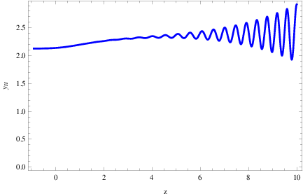
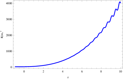
The function is by itself a statefinder parameter for the dark energy era, and in fact was used indirectly in Ref. Sahni:2014ooa to discuss the issue that it might become negative at a redshift firstly reported in Ref. Delubac:2014aqe. Basically, good statefinder parameters are those associated with the geometry of the spacetime, thus the Hubble rate and its higher derivatives. Also it is known that the gravity models that can describe a dynamical dark energy era, are plagued with the problem of dark energy oscillations at high redshift , and singularities in the dark energy EoS parameter may occur during the matter domination era. In our case, the term cures these singularities, as it is already known in the literature that such a term amends the singularities issue in the dark energy EoS Appleby:2009uf; Bamba:2008ut, but the dark energy oscillations issue still remains. In fact, as we will show, the oscillations issue becomes more evident in statefinder parameters that contain higher derivatives of the Hubble rate, and is strongly affected by the initial conditions chosen for , thus it is affected by the parameter appearing in Eqs. (42). Let us solve numerically the differential equation (39), for the values of the parameters defined in this and the previous sections, with the initial conditions (42), for . In the left plot of Fig. 1 we present the behavior of the function as a function of the redshift, and already the issue of dark energy oscillations becomes apparent for redshifts and higher. In the right plot of Fig. 1 we present the behavior of the scalar curvature (41) as a function of the redshift.
In order to better understand the behavior of the model and assess the viability of the model, we shall compare several statefinder quantities for the model and directly compare these to the CDM model values. We start off with the dark energy EoS parameter , which can be expressed in terms of the function as follows,
| (44) |
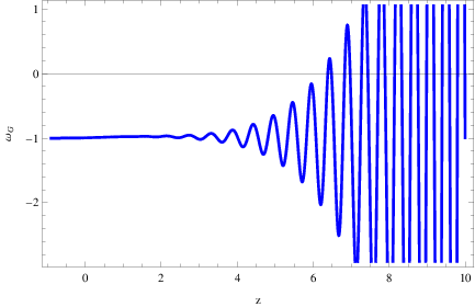
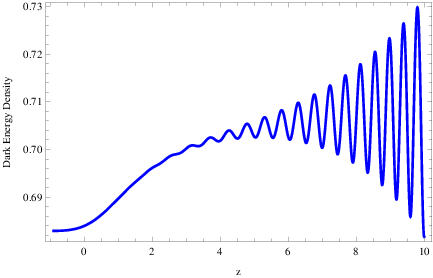
which is also a good statefinder since it depends on the geometry via the dependence on the derivatives of the Hubble rate . In the left plot of Fig. 2 we present the behavior of the dark energy EoS for . As it can be seen, the EoS parameter for the model has oscillating behavior for approximately, but the present day value is , which is compatible with the latest Planck constraints Aghanim:2018eyx, which is . The results for present day values of the various parameters that will be obtained hereafter, are summarized in Table 1. Also in the right plot of Fig. 2 we plot , as a function of the redshift, and is written as a function of the function as follows,
| (45) |
As it can be seen in the right plot of Fig. 2, the late-time behavior of is oscillation-free and leads to the present day value prediction , which is also compatible with the latest Planck constraint .
The statefinder quantities as we already mentioned, are quite important since the results depict the effects of the geometry of spacetime on the statefinder quantities, and this is why the statefinder quantities are valuable tools for late-time cosmology. We shall be interested in four statefinder quantities, namely the deceleration parameter , the jerk , the parameter Sahni:2002fz and finally the parameter Sahni:2014ooa, which their functional behavior as functions of the Hubble rate is given below,
| (46) | ||||
The last three, namely the jerk , and have very simple values for the CDM model, which are , and . We can easily compare the results of the axion gravity model with those of the CDM by expressing the statefinders (46) as functions of the redshift, but the final expressions are too lengthy to quote here. The results of the numerical integration are shown in Figs. 3, where in the upper left the deceleration parameter of the axion gravity model is plotted as a function of the redshift (blue curve) and the corresponding deceleration parameter of the CDM model also appears (red). As it can be seen, these are indistinguishable up to a redshift . In the upper right of Fig. 3 , in the lower left we plot the jerk and in the lower right plot the statefinder for the axion model and for the CDM is shown. In all the plots, the red curve corresponds to the CDM model, and the blue curve to the axion gravity model, for . As it can be seen in the upper plots of Fig. 3, when lower derivatives of the Hubble rate are invoked, or even simply of the Hubble rate in the case of the statefinder , the oscillations of the dark energy at higher redshifts are not so pronounced. However, it is notable that the CDM and the axion gravity model can be distinguished even at low redshifts when the statefinder is considered. From the lower plots of Fig. 3 it is evident that when higher derivatives of the Hubble rate are invoked, the dark energy oscillations are strongly pronounced even for redshift values and higher, as we already expected. However, the low redshift behavior of the statefinders and are similar to the ones corresponding to the CDM model.
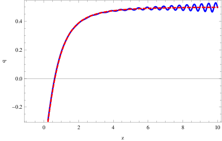
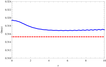
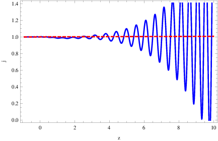
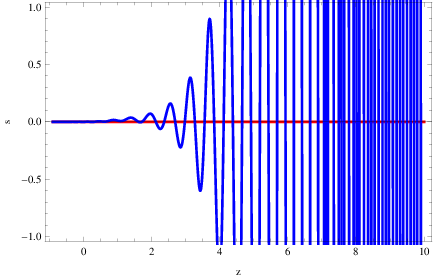
We need to note though, that although the dark energy oscillations are apparent especially in more complex statefinder parameters, the term in the gravity of Eq. (2) ensures the absence of singularities in the dark energy EoS parameter, as is also noted in the literature Appleby:2009uf. In fact, this can also be seen in the left plot of Fig. 2, since the oscillations of dark energy are not so pronounced, in comparison to statefinders containing higher derivatives of the Hubble rate. The results of the values of the statefinders at present time and the comparison the the values of the CDM model can be found in Table 1.
| Cosmological Parameter | Axion Gravity Value | Base CDM or Planck 2018 Value |
|---|---|---|
| 0.683948 | ||
| -0.995205 | ||
| 0.319364 | ||
| -0.520954 | -0.535 | |
| 1.00319 | 1 | |
| -0.00104169 | 0 |
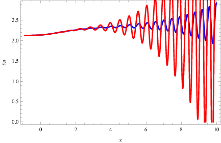
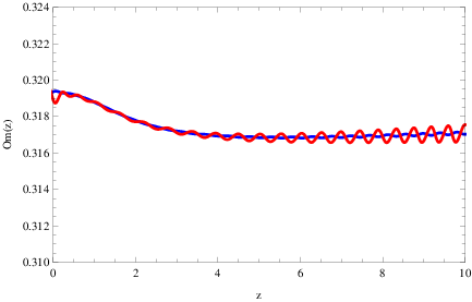
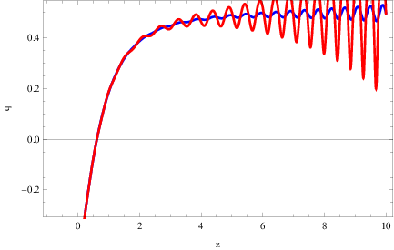
Another important issue we need to discuss is the effect of the initial conditions on the phenomenology of the axion gravity model. We performed the numerical integration of the differential equation (39) with the initial conditions (42) for two values of , namely and . The results are quite interesting since the effect of the initial conditions on the values of the physical parameters and on the statefinders at present time is minor, apart from the ones that contain higher derivatives of the Hubble rate, namely and , but the changes are of the order . For a direct comparison we quote these on Table 2. However, the effect of the values of and in effect of the initial conditions on the dark energy oscillations is mentionable, and in fact, as takes larger values, the oscillations are more pronounced. This can be seen in Fig. 4, where we present the behavior of the deceleration parameter , of the statefinder and of the function as a function of the redshift, for (red curves) and for (blue curves). Also for even smaller values of , the oscillation behavior is even less pronounced.
| Cosmological Parameter | Axion Gravity Value | Base CDM or Planck 2018 Value |
|---|---|---|
| 0.683968 | ||
| -0.995827 | ||
| 0.318919 | ||
| -0.521621 | -0.535 | |
| 0.980965 | 1 | |
| 0.00621087 | 0 |
In conclusion, we demonstrated that the axion gravity model can mimic the CDM model at late-times and can also provide a viable late-time phenomenology compatible with the Planck 2018 constraints on the cosmological parameters quantifying the effects of the dark energy. However, the issue of dark energy oscillations seems to be present, as was expected though. The dark energy oscillations are strongly affected by the initial conditions chosen for the function and its derivative during the last stages of the matter domination era, however we will report soon on a mechanism that may eliminate completely the dark energy oscillations from gravity models.
At this point, let us investigate whether the gravity model satisfies the viability criteria that any gravity model should satisfy. These are,
| (47) |
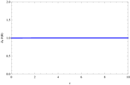
for , where is the present day curvature. In Fig. 5 we plot the behavior of and as functions of the redshift, for small redshifts, and the same applies for higher redshifts. In fact, when , then and we have approximately eV-1, and , thus the viability conditions are satisfied even up to inflationary scales.
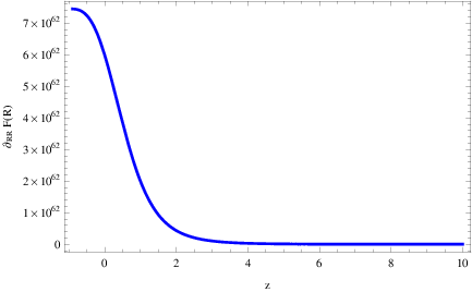
Before closing, we need to note that in Ref. Odintsov:2017hbk we also proposed an gravity in which the functional form of the gravity was chosen in such a way so that the dark energy oscillations in large redshifts are reduced or eliminated. The action in the case of Ref. Odintsov:2017hbk was of the form,
| (48) |
where,
| (49) |
with being a positive parameter and being the cosmological constant. In addition, the function is,
| (50) |
with being a real and positive. The choice of the function is crucial for the stabilization of the theory at large redshifts, and it is basically a deformed correction. As was shown in Ref. Odintsov:2017hbk, such a stabilization is achieved in this case, but we do not perform this analysis in this paper.
IV Concluding Remarks
In this work we considered an axion gravity model, in which the axion eventually is the main component of cold dark matter in the Universe, and we demonstrated that the axion gravity model can unify the early-time with the late-time acceleration. We chose the gravity to contain an term and also a term with , with the term being motivated for a viable description of the inflationary era, while the term was added for a successful description of the late-time acceleration era. The axion scalar field was described by a canonical scalar field with a broken primordial Peccei-Quinn symmetry, in the context of the misalignment axion scenario. During the inflationary era, the axion scalar was frozen in its primordial vacuum expectation value, and thus it merely contributes a cosmological constant in the gravitational equations of motion. In effect, the term of the gravity controls the primordial dynamics, and it generates a viable acceleration era. We quantified these considerations and we demonstrated that indeed the axion and the terms have a minor contribution to the dynamics of the model. As the Universe expands though, when and for , the axion starts to oscillate. Assuming a slowly varying oscillation for the axion, we demonstrated that the axion energy density scales as , thus the axion scalar mimics the dark matter fluid, with an average EoS parameter . At late times, the gravity term controls the dynamics of the model, via its first derivatives, but we needed to quantify this in the best way we could, so we used numerical analysis to solve the Friedmann equation. We introduced a statefinder function which is the fraction of the dark energy energy density over the current cold dark matter energy density , and we rewritten the Friedmann equation in terms of . By using appropriate initial conditions, we numerically solved the Friedmann equation, and we focused our analysis up to redshift . We focused our analysis on the behavior of statefinder quantities, and also on the energy density of dark energy and its EoS behavior. We found that the gravity model produces results very similar to the CDM model, in some cases almost identical for small redshifts, and in all cases compatible results with the latest Planck constraints on the cosmological parameters. In addition, we showed that for statefinder quantities that contain higher derivatives of the Hubble rate, the dark energy oscillations issue occurs, as expected. This oscillation issue is more pronounced for larger redshifts, and is strongly affected by the initial conditions we used. However, the presence of the term ensures the absence of singularities in the dark energy EoS parameter, nevertheless this issue of oscillations, somewhat obscures the whole picture. In response to this issue, in a future work we shall present how the oscillations can be eliminated from the gravity late-time phenomenology.
Another issue we did not address is related to the reheating era. In the axion gravity model we present, this is expected to be somewhat complicated, and not so easy to address analytically, due to the presence of and terms caused by the axion and the gravity in the Friedmann equation. In principle, the term is not expected to be dominant in this era, since the curvature is already too small, and the axion already starts to oscillate in a slowly-varying way. This study is an important one, which we hope to address in a future work focused on this issue.
Another issue that is quite interesting and valuable for future observations, of matter curvature perturbations for the gravity axion model. In the presence of gravity, Newton’s effective gravitational constant is different from the present day value, during the matter domination era, however, the axion also contributes to the matter curvature perturbations. The question is which contribution is dominant and to which extent. The study for the axion effect on the matter curvature perturbations was performed in Choi:1999zy; Hwang:2009js; Park:2012ru; Noh:2013coa; Noh:2015spa, while for the gravity case see Bamba:2012qi. The evolution of the matter curvature perturbations is valuable phenomenologically, since the growth index is an observable that may even discriminate modified gravities between them.
A highly non-trivial issue is the axion isocurvature perturbations issue, generated during or mainly well after the first horizon crossing and before the horizon re-entry. Although misalignment axion scalars have minor backreaction from isocurvature perturbations during inflation, if these are generated well after the first horizon crossing, might have an observable effect. The question is to what extent may gravity affect the generation of axion isocurvature perturbations and their evolution. This is a highly non-trivial issue to address, and we leave this open as question.
Finally, it is noteworthy another phenomenologically interesting issue, which deserves to be addressed in detail in a future work. It is related to the fact that in some observational data Sahni:2014ooa; Delubac:2014aqe, these suggest that the function took negative values during the last stages of the matter domination era, and specifically around . This is a highly intriguing issue, and we devised a mechanism in the context of modified gravity in order to produce both a viable late-time era at and a negative , without introducing compensating dark energy mechanisms. We shall report on this intriguing issue in the near future.
Acknowledgments
This work is supported by MINECO (Spain), FIS2016-76363-P, and by project 2017 SGR247 (AGAUR, Catalonia) (S.D.O), and by Russian Ministry of Science and High Education, project No. 3.1386.2017.
References
- (1) A. G. Riess et al. [Supernova Search Team], Astron. J. 116 (1998) 1009 [astro-ph/9805201].
- (2) N. Aghanim et al. [Planck Collaboration], arXiv:1807.06209 [astro-ph.CO].
- (3) A. G. Riess et al., Astrophys. J. 730 (2011) 119 Erratum: [Astrophys. J. 732 (2011) 129] [arXiv:1103.2976 [astro-ph.CO]].
- (4) V. C. Busti, C. Clarkson and M. Seikel, Mon. Not. Roy. Astron. Soc. 441 (2014) 11 [arXiv:1402.5429 [astro-ph.CO]].
- (5) V. Sahni, A. Shafieloo and A. A. Starobinsky, Astrophys. J. 793 (2014) no.2, L40 [arXiv:1406.2209 [astro-ph.CO]].
- (6) S. Nojiri, S. D. Odintsov and V. K. Oikonomou, Phys. Rept. 692 (2017) 1 [arXiv:1705.11098 [gr-qc]].
- (7)
S. Capozziello, M. De Laurentis,
Phys. Rept. 509, 167 (2011);
V. Faraoni and S. Capozziello, Fundam. Theor. Phys. 170 (2010). - (8) S. Nojiri, S.D. Odintsov, eConf C0602061, 06 (2006) [Int. J. Geom. Meth. Mod. Phys. 4, 115 (2007)].
- (9) S. Nojiri, S.D. Odintsov, Phys. Rept. 505, 59 (2011);
- (10) A. de la Cruz-Dombriz and D. Saez-Gomez, Entropy 14 (2012) 1717 [arXiv:1207.2663 [gr-qc]].
- (11) G. J. Olmo, Int. J. Mod. Phys. D 20 (2011) 413 [arXiv:1101.3864 [gr-qc]].
- (12) S. Capozziello, Int. J. Mod. Phys. D 11 (2002) 483 [gr-qc/0201033]
- (13) S. M. Carroll, V. Duvvuri, M. Trodden and M. S. Turner, Phys. Rev. D 70 (2004) 043528 [astro-ph/0306438].
- (14) S. Nojiri and S. D. Odintsov, Phys. Rev. D 68 (2003) 123512 [hep-th/0307288].
- (15) S. Nojiri and S. D. Odintsov, Phys. Lett. B 657 (2007) 238 [arXiv:0707.1941 [hep-th]].
- (16) S. Nojiri and S. D. Odintsov Phys. Rev. D 77 (2008) 026007 [arXiv:0710.1738 [hep-th]].
- (17) G. Cognola, E. Elizalde, S. Nojiri, S. D. Odintsov, L. Sebastiani and S. Zerbini, Phys. Rev. D 77 (2008) 046009 [arXiv:0712.4017 [hep-th]].
- (18) S. Nojiri and S. D. Odintsov, Phys. Rev. D 74 (2006) 086005 [hep-th/0608008].
- (19) M. Benetti and S. Capozziello, arXiv:1910.09975 [astro-ph.CO].
- (20) V. K. Oikonomou, J. D. Vergados and C. C. Moustakidis, Nucl. Phys. B 773 (2007) 19 [hep-ph/0612293].
- (21) D. J. E. Marsh, Phys. Rept. 643 (2016) 1 [arXiv:1510.07633 [astro-ph.CO]].
- (22) P. Sikivie, Lect. Notes Phys. 741 (2008) 19 [astro-ph/0610440].
- (23) G. G. Raffelt, Lect. Notes Phys. 741 (2008) 51 [hep-ph/0611350].
- (24) A. D. Linde, Phys. Lett. B 259 (1991) 38.
- (25) M. C. D. Marsh, H. R. Russell, A. C. Fabian, B. P. McNamara, P. Nulsen and C. S. Reynolds, JCAP 1712 (2017) no.12, 036 [arXiv:1703.07354 [hep-ph]].
- (26) S. D. Odintsov and V. K. Oikonomou, Phys. Rev. D 99 (2019) no.6, 064049 [arXiv:1901.05363 [gr-qc]].
- (27) S. Nojiri, S. D. Odintsov, V. K. Oikonomou and A. A. Popov, Phys. Rev. D 100 (2019) no.8, 084009 [arXiv:1909.01324 [gr-qc]].
- (28) S. Nojiri, S. D. Odintsov and V. K. Oikonomou, arXiv:1907.01625 [gr-qc].
- (29) S. D. Odintsov and V. K. Oikonomou, Phys. Rev. D 99 (2019) no.10, 104070 [arXiv:1905.03496 [gr-qc]].
- (30) M. Cicoli, V. Guidetti and F. G. Pedro, arXiv:1903.01497 [hep-th].
- (31) H. Fukunaga, N. Kitajima and Y. Urakawa, arXiv:1903.02119 [astro-ph.CO].
- (32) A. Caputo, arXiv:1902.02666 [hep-ph].
- (33) A.S.Sakharov and M.Yu.Khlopov, Yadernaya Fizika (1994) V. 57, PP. 514- 516. ( Phys.Atom.Nucl. (1994) V. 57, PP. 485-487); A.S.Sakharov, D.D.Sokoloff and M.Yu.Khlopov, Yadernaya Fizika (1996) V. 59, PP. 1050-1055. (Phys.Atom.Nucl. (1996) V. 59, PP. 1005-1010); M .Yu.Khlopov, A.S.Sakharov and D.D.Sokoloff, Nucl.Phys. B (Proc. Suppl.) (1999) V. 72, 105-109.
- (34) J. H. Chang, R. Essig and S. D. McDermott, JHEP 1809 (2018) 051 [arXiv:1803.00993 [hep-ph]]. Chang:2018rso,Irastorza:2018dyq,
- (35) I. G. Irastorza and J. Redondo, Prog. Part. Nucl. Phys. 102 (2018) 89 [arXiv:1801.08127 [hep-ph]].
- (36) V. Anastassopoulos et al. [CAST Collaboration], Nature Phys. 13 (2017) 584 [arXiv:1705.02290 [hep-ex]].
- (37) P. Sikivie, Phys. Rev. Lett. 113 (2014) no.20, 201301 [arXiv:1409.2806 [hep-ph]].
- (38) P. Sikivie, Phys. Lett. B 695 (2011) 22 [arXiv:1003.2426 [astro-ph.GA]].
- (39) P. Sikivie and Q. Yang, Phys. Rev. Lett. 103 (2009) 111301 [arXiv:0901.1106 [hep-ph]].
- (40) A. Caputo, L. Sberna, M. Frias, D. Blas, P. Pani, L. Shao and W. Yan, Phys. Rev. D 100 (2019) no.6, 063515 [arXiv:1902.02695 [astro-ph.CO]].
- (41) E. Masaki, A. Aoki and J. Soda, arXiv:1909.11470 [hep-ph].
- (42) J. Soda and D. Yoshida, Galaxies 5 (2017) no.4, 96.
- (43) J. Soda and Y. Urakawa, Eur. Phys. J. C 78 (2018) no.9, 779 [arXiv:1710.00305 [astro-ph.CO]].
- (44) A. Aoki and J. Soda, Phys. Rev. D 96 (2017) no.2, 023534 [arXiv:1703.03589 [astro-ph.CO]].
- (45) E. Masaki, A. Aoki and J. Soda, Phys. Rev. D 96 (2017) no.4, 043519 [arXiv:1702.08843 [astro-ph.CO]].
- (46) A. Aoki and J. Soda, Int. J. Mod. Phys. D 26 (2016) no.07, 1750063 [arXiv:1608.05933 [astro-ph.CO]].
- (47) I. Obata and J. Soda, Phys. Rev. D 94 (2016) no.4, 044062 [arXiv:1607.01847 [astro-ph.CO]].
- (48) A. Aoki and J. Soda, Phys. Rev. D 93 (2016) no.8, 083503 [arXiv:1601.03904 [hep-ph]].
- (49) T. Ikeda, R. Brito and V. Cardoso, Phys. Rev. Lett. 122 (2019) no.8, 081101 [arXiv:1811.04950 [gr-qc]].
- (50) A. Arvanitaki, S. Dimopoulos, M. Galanis, L. Lehner, J. O. Thompson and K. Van Tilburg, arXiv:1909.11665 [astro-ph.CO].
- (51) A. Arvanitaki, M. Baryakhtar, S. Dimopoulos, S. Dubovsky and R. Lasenby, Phys. Rev. D 95 (2017) no.4, 043001 [arXiv:1604.03958 [hep-ph]].
- (52) A. Arvanitaki, M. Baryakhtar and X. Huang, Phys. Rev. D 91 (2015) no.8, 084011 [arXiv:1411.2263 [hep-ph]].
- (53) A. Arvanitaki and A. A. Geraci, Phys. Rev. Lett. 113 (2014) no.16, 161801 [arXiv:1403.1290 [hep-ph]].
- (54) S. Sen, Phys. Rev. D 98 (2018) no.10, 103012 [arXiv:1805.06471 [hep-ph]].
- (55) V. Cardoso, S. J. C. Dias, G. S. Hartnett, M. Middleton, P. Pani and J. E. Santos, JCAP 1803 (2018) 043 [arXiv:1801.01420 [gr-qc]].
- (56) J. G. Rosa and T. W. Kephart, Phys. Rev. Lett. 120 (2018) no.23, 231102 [arXiv:1709.06581 [gr-qc]].
- (57) H. Yoshino and H. Kodama, PTEP 2014 (2014) 043E02 [arXiv:1312.2326 [gr-qc]].
- (58) C. S. Machado, W. Ratzinger, P. Schwaller and B. A. Stefanek, arXiv:1912.01007 [hep-ph].
- (59) A. Korochkin, A. Neronov and D. Semikoz, arXiv:1911.13291 [hep-ph].
- (60) A. S. Chou, Astrophys. Space Sci. Proc. 56 (2019) 41.
- (61) C. F. Chang and Y. Cui, arXiv:1911.11885 [hep-ph].
- (62) N. Crisosto, G. Rybka, P. Sikivie, N. S. Sullivan, D. B. Tanner and J. Yang, arXiv:1911.05772 [astro-ph.CO].
- (63) K. Choi, H. Seong and S. Yun, arXiv:1911.00532 [hep-ph].
- (64) M. Kavic, S. L. Liebling, M. Lippert and J. H. Simonetti, arXiv:1910.06977 [astro-ph.HE].
- (65) D. Blas, A. Caputo, M. M. Ivanov and L. Sberna, arXiv:1910.06128 [hep-ph].
- (66) D. Guerra, C. F. B. Macedo and P. Pani, JCAP 1909 (2019) no.09, 061 [arXiv:1909.05515 [gr-qc]].
- (67) T. Tenkanen and L. Visinelli, JCAP 1908 (2019) 033 [arXiv:1906.11837 [astro-ph.CO]].
- (68) G. Y. Huang and S. Zhou, Phys. Rev. D 100 (2019) no.3, 035010 [arXiv:1905.00367 [hep-ph]].
- (69) D. Croon, R. Houtz and V. Sanz, JHEP 1907 (2019) 146 [arXiv:1904.10967 [hep-ph]].
- (70) F. V. Day and J. I. McDonald, JCAP 1910 (2019) no.10, 051 [arXiv:1904.08341 [hep-ph]].
- (71) N. Du et al. [ADMX Collaboration], Phys. Rev. Lett. 120 (2018) no.15, 151301 [arXiv:1804.05750 [hep-ex]].
- (72) R. Henning et al. [ABRACADABRA Collaboration],
- (73) J. L. Ouellet et al., arXiv:1810.12257 [hep-ex].
- (74) B. R. Safdi, Z. Sun and A. Y. Chen, arXiv:1811.01020 [astro-ph.CO].
- (75) M. Rozner, E. Grishin, Y. B. Ginat, A. P. Igoshev and V. Desjacques, arXiv:1904.01958 [gr-qc].
- (76) F. T. Avignone, R. J. Creswick and J. D. Vergados, arXiv:1801.02072 [hep-ph].
- (77) A. Caputo, M. Regis, M. Taoso and S. J. Witte, arXiv:1811.08436 [hep-ph].
- (78) A. Caputo, C. P. Garay and S. J. Witte, Phys. Rev. D 98 (2018) no.8, 083024 [arXiv:1805.08780 [astro-ph.CO]].
- (79) M. Lawson, A. J. Millar, M. Pancaldi, E. Vitagliano and F. Wilczek, arXiv:1904.11872 [hep-ph].
- (80) A. B. Balakin and W. T. Ni, Class. Quant. Grav. 27 (2010) 055003 [arXiv:0911.2946 [gr-qc]].
- (81) A. B. Balakin, V. V. Bochkarev and N. O. Tarasova, Eur. Phys. J. C 72 (2012) 1895 [arXiv:1201.3009 [gr-qc]].
- (82) A. B. Balakin, R. K. Muharlyamov and A. E. Zayats, Eur. Phys. J. D 68 (2014) 159 [arXiv:1404.4479 [gr-qc]].
- (83) M. Satoh, S. Kanno and J. Soda, Phys. Rev. D 77 (2008) 023526 [arXiv:0706.3585 [astro-ph]].
- (84) K. Inomata and M. Kamionkowski, Phys. Rev. Lett. 123 (2019) no.3, 031305 [arXiv:1811.04959 [astro-ph.CO]].
- (85) M. Kamionkowski and A. H. Jaffe, Int. J. Mod. Phys. A 16S1A (2001) 116 [ICTP Lect. Notes Ser. 3 (2001) 415] [astro-ph/0011329].
- (86) F. D’Eramo, R. Z. Ferreira, A. Notari and J. L. Bernal, JCAP 1811 (2018) 014 [arXiv:1808.07430 [hep-ph]].
- (87) M. Dine and A. Anisimov, JCAP 0507 (2005) 009 [hep-ph/0405256].
- (88) S. A. Appleby, R. A. Battye and A. A. Starobinsky, JCAP 1006 (2010) 005 [arXiv:0909.1737 [astro-ph.CO]].
- (89) W. Hu and I. Sawicki, Phys. Rev. D 76 (2007) 064004 [arXiv:0705.1158 [astro-ph]].
- (90) K. Bamba, A. Lopez-Revelles, R. Myrzakulov, S. D. Odintsov and L. Sebastiani, Class. Quant. Grav. 30 (2013) 015008 [arXiv:1207.1009 [gr-qc]].
- (91) T. Delubac et al. [BOSS Collaboration], Astron. Astrophys. 574 (2015) A59 [arXiv:1404.1801 [astro-ph.CO]].
- (92) K. Bamba, S. Nojiri and S. D. Odintsov, JCAP 0810 (2008) 045 [arXiv:0807.2575 [hep-th]].
- (93) V. Sahni, T. D. Saini, A. A. Starobinsky and U. Alam, JETP Lett. 77 (2003) 201 [Pisma Zh. Eksp. Teor. Fiz. 77 (2003) 249] [astro-ph/0201498].
- (94) S. D. Odintsov, V. K. Oikonomou and L. Sebastiani, Nucl. Phys. B 923 (2017) 608 doi:10.1016/j.nuclphysb.2017.08.018 [arXiv:1708.08346 [gr-qc]].
- (95) K. Choi, J. c. Hwang and K. W. Hwang, Phys. Rev. D 61 (2000) 084026 [hep-ph/9907244].
- (96) J. c. Hwang and H. Noh, Phys. Lett. B 680 (2009) 1 [arXiv:0902.4738 [astro-ph.CO]].
- (97) C. G. Park, J. c. Hwang and H. Noh, Phys. Rev. D 86 (2012) 083535 [arXiv:1207.3124 [astro-ph.CO]].
- (98) H. Noh, C. G. Park and J. c. Hwang, Phys. Lett. B 726 (2013) 559 [arXiv:1309.5692 [astro-ph.CO]].
- (99) H. Noh, J. c. Hwang and C. G. Park, JCAP 1512 (2015) 016 [arXiv:1509.00937 [gr-qc]].