An étude of momentum space scalar amplitudes in AdS
Soner Albayraka,b, Chandramouli Chowdhuryc, and Savan Khareld
Department of Physics, Yale University, New Haven, CT 06511
Walter Burke Institute for Theoretical Physics, Caltech, Pasadena, CA 91125
International Centre for Theoretical Sciences, Tata Institute of Fundamental Research, Sivakote, Bangalore 560089, INDIA
Department of Physics, Williams College, Williamstown, MA 01267
Abstract
In this paper, we explore momentum space approach to computing scalar amplitudes in Anti-de Sitter space. We show that the algorithm derived by Arkani-Hamed, Benincasa, and Postnikov for cosmological wavefunctions can be straightforwardly adopted for AdS transition amplitudes in momentum space, allowing one to bypass bulk point integrations. We demonstrate the utility of this approach in AdS by presenting several explicit results both at tree and loop level.
1 Introduction
In the last decade, there has been a resurrection in the study of scattering amplitudes and conformal correlation functions. Such undertakings have extricated rich structures of quantum field theory and quantum gravity. In particular, we now have considerable evidence that scattering amplitudes in quantum gravity can be computed from the correlation functions in one lower dimensions. Such a correspondence is known as the holographic duality [1, 2, 3] and its most concrete formalism in given by AdS/CFT where the bulk geometry is Anti de Sitter space and the conformal correlation functions live at the boundary. This correspondence has led to major insights into the nature of quantum gravity as well as gauge theory.
Besides yielding useful insights, holographic correlators have been discovered to have rich mathematical structures [4, 5, 6, 7, 8, 9, 10, 11, 12, 13, 14, 15, 16, 17, 18, 19, 20, 21, 22, 23, 24, 25, 26, 27, 28, 29, 30, 31, 32]. However, momentum-space methods, our usual modus operandi of doing computation in quantum field theory, is still not yet fully studied for CFTs (see for a partial list of progress [33, 34, 35, 36, 37, 38, 39, 40, 41, 42, 43, 44, 45, 46, 47, 48, 49, 50, 51, 52, 53, 54, 55, 56, 57, 58]). We also now know that the usual scattering amplitudes arise from the flat space limit of the holographic Conformal Field Theory (CFT) correlators. Hence it is useful to generalize the tools that have been developed for the usual scattering amplitudes in flat space to holographic correlators. A modest step in this direction is taken in [59] where it is shown that tree level gauge theory Witten diagrams for transition amplitudes, reduce to surprisingly simple expressions when expressed in momentum space.11 1 Transition amplitudes are generalizations of vacuum-correlators such that one replaces some of the bulk to boundary propagators of the relevant Witten diagram with normalizable modes [37]. Such a replacement roughly creates the effect of changing the boundary conditions at past and future horizons of the relevant Poincaré patch, creating past and future states for the correlator (hence the name transition amplitude). In a similar vein, momentum space approach to transition amplitudes also simplifies the computation of graviton exchange diagrams, which was demonstrated in [60] with explicit higher point tree level results.
The momentum space formalism for AdS calculations can be upgraded with a new algorithm developed by Arkani-Hamed, Benincasa, and Postnikov in [61] where they investigate the wavefunction of the Universe in de Sitter background. Indeed, it was realized in [62] that the computation of gluon Witten diagrams in AdS4 can actually use the same combinatorial relations developed in [61] if it is written in momentum space. This correspondence allowed the authors to compute any tree level gluon exchange diagram algebraically, without having to do any explicit bulk integrations.
In this paper, we would like to extend this marriage between Arkani-Hamed et al’s algorithm and AdS momentum space beyond AdS4 gluons. We will show that conformally coupled scalars in any AdSd+1 can be computed algorithmically, both at tree and loop level, and we will demonstrate this with explicit results for various Witten diagrams. Besides its formal usage, the AdS transition amplitudes can be useful in the computation of the wave function at late times from which one can compute de Sitter correlators [63, 64]. The growing interest in cosmology has generated a great deal of excitement in the study of late time de Sitter correlators [65, 66, 67, 68, 69, 70, 71, 38, 72, 73, 74, 75, 76, 77, 50, 78, 79, 80, 81, 82, 83, 84] and we believe that the analogous calculations of momentum space AdS amplitudes can assist in the study of the shape of non-Gaussianities.
Here is the organization of the paper. In section 2, we discuss scalars in curved spacetime and present the review of momentum space toolkit in Anti-de Sitter space. We also demonstrate the standard non-algorithmic approach of momentum space formalism by computing Witten diagrams for minimally coupled scalars. In section 3, we switch to conformally coupled scalars, discuss how the algorithmic approach works, and provide explicit results both at tree and loop levels. Finally, we conclude with a brief discussion and future directions.
2 Preliminaries
2.1 Scalars in curved spacetime
A free scalar in flat space satisfies the Klein-Gordon equation which reads as
| (2.1) |
where is the mass parameter of the field. In curved spacetime, this equation becomes
| (2.2) |
where is the Ricci scalar and is a coefficient determining the interaction between scalar and the background. In the case of AdSd+1, this equation follows from the action
| (2.3) |
where and we stick to mostly positive metric convention throughout the paper.
The scalar in curved spacetime has been extensively analyzed in the literature; however, the analysis usually focus on two specific values of : minimally coupled scalar with , and conformally coupled scalar with for
| (2.4) |
The popularity of minimally coupled scalar follows from the fact that simplifies the Lagrangian. The appeal of conformally-coupled scalar, however, cannot be immediately seen unless one goes to local Minkowski frame where the potential term takes the form [85]
| (2.5) |
One sees that if (in addition to ) one imposes , the potential vanishes, leading the theory to enjoy conformal symmetry. Indeed, even though all pairs fall into the class of conformally coupled scalars, only case is invariant under conformal transformations [86].
Tuning the parameters is necessary for the theory to enjoy conformal symmetry but it is not sufficient: we also need to check if the interaction Lagrangian spoils this symmetry. As a prerequisite condition of scale invariance we restrict to interactions of the form which transforms as as for constant .
In this paper, we focus on non-derivative interactions for which the action takes the form
| (2.6) |
We can check the trace of stress tensor to see when it is zero. Indeed, via
| (2.7) |
we obtain
| (2.8) |
where we used
| (2.9) |
for whose derivation with a nice explanation we suggest the lecture notes of Matthias Blau, available at http://www.blau.itp.unibe.ch/newlecturesGR.pdf.22 2 This equation is actually true only if there are no contributions at the boundary as its derivation uses integration by parts and assumes that total derivative terms do not contribute. Strictly speaking, this is not correct for AdS. However, boundary conditions actually kill the additional piece unless the variation of the action on the boundary contains the derivative of the variation of the boundary metric for which one then needs to add an appropriate boundary term to cancel the additional variation, see [87] in the case of Einstein gravity. We will avoid such subtleties (and refer reader to [88, 89] and references therein) so a rigorous minded reader should see our calculations not as a derivation but as a motivation for why only certain interactions can enjoy full conformal symmetry.
The trace of stress tensor then reads as
| (2.10) |
We see the first term dies only if . We can then kill the second term with equation of motion if and for
| (2.11) |
e.g. for AdS4. We thus arrived at the well-known conclusion: the action in eqn. (2.6) enjoys conformal symmetry only if .
We can derive this result from another, and slightly simpler, approach. We first specialize to the AdS with the Poincaré metric and the Ricci scalar
| (2.12) |
where we take AdS radius in the rest of the paper.33 3 Our notation is such that is the radial coordinate and the transverse coordinates approach to the boundary coordinate as . We then consider a Weyl transformation which maps AdS to flat space:
| (2.13a) | ||||
| (2.13b) | ||||
where we used the engineering scaling dimension for the scalar field. Under this transformation, quadratic part which is invariant under conformal transformations map to the free scalar in flat space
| (2.14a) | |||
| whereas the interaction part maps as | |||
| (2.14b) | |||
We immediately see that we need if we require the flat space interaction to be conformally invariant as well.
2.2 Review of momentum space toolkit in AdS
In this section, we will review the basics of our framework and specifics regarding the scalars. For similar reviews in the context of gauge fields and gravitons, see [59, 62, 60].
We will be working with the Poincaré patch of eqn. (2.12) and take the Fourier transform of . We will leave as it is though: the coordinates are what we call the momentum space in this paper. This is in the same spirit of the treatment in [35, 37, 33].
In momentum space, equation of motion in eqn. (2.2) becomes
| (2.15) |
where we define the effective mass square
| (2.16) |
The general solution to this differential equation for timelike momenta reads as:44 4 Here, () is the Bessel function of the first (second) kind.
| (2.17) |
where we define
| (2.18) |
and where .55 5 We specifically chose the letter to denote as this term up to an overall is the pole of the spectral representation of the bulk to bulk propagator, usually denoted as in the literature [90], where there are two poles due to the shadow symmetry.,66 6 The scaling dimension of the dual operator in the boundary CFT is in our notation. We would like to caution the reader that many papers in literature calls mass what we defined as the effective mass , hence the well-known formula , which becomes in our notation. As we choose to distinguish mass and effective mass , it is completely consistent in our definition when we say massless conformally coupled scalar as despite .
For spacelike momenta, the regularity in the AdS can only be achieved for the particular combination which sums up to the Bessel function of the second kind, i.e.
| (2.19) |
Note that this is always possible due to the identity77 7 This is only true for . For generic , the relevant identity reads as (2.20)
| (2.21) |
Below, we will focus on massless minimally coupled scalars and massless conformally coupled scalars for which the relevant bulk to boundary propagators read as
| (2.22a) | ||||
| (2.22b) | ||||
where we use the fact that Ricci scalar in AdS.
We can similarly calculate the bulk to bulk propagators. We are looking for the solutions to the equation
| (2.23) |
We observe that
| (2.24) |
and since we also have the identity
| (2.25) |
we find the propagator:
| (2.26) |
In particular, gives the propagator for conformally (minimally) coupled scalar as we noted above.
One can now go ahead and write the expression for Witten diagrams. At tree level, the amplitude for a diagram of external legs and bulk propagators reads as
| (2.27) |
for the interaction coefficient at vertex, where and , and where are norms of linear combinations of vectors depending on the topology.
As an example, we can consider the topology in Figure 1 for minimally coupled scalars; the relevant amplitude would read as
| (2.28) |
where we are following the notation of [59] for addition of vectors.88 8 Explicitly: (2.29a) and (2.29b) For example, and .

2.3 Example: minimally coupled scalars in AdS4
In this section we will calculate some amplitudes for tree level Witten diagrams using the procedure advocated in the previous section; specifically, with
| (2.31) | ||||
where we choose a particular normalization for the bulk to boundary propagator consistent with the literature.99 9 An overall dependent scaling of bulk to boundary propagators, i.e. , is immaterial for our purposes in this paper, hence we refer this as a normalization and fix it with a convenient factor. However, this normalization is actually tightly constrained by scaling dimensions of the dual operators at the boundary CFT.
Apart from its physical significance, we focus on AdS4 also because Bessel functions simplify for half integer arguments; hence the calculations are relatively easier for AdS2+2n. This motivation was also used in previous similar work [59, 62, 60], where the calculation of graviton amplitudes in [60] is actually quite similar to the computation at hand. Specially, one can write the graviton propagators in AdSd+1 as
| (2.32) | ||||
where is a differential operator whose details are irrelevant for us. However, one important remark is that these differential operators commute with the rest of the calculation, thus for a Witten diagram with bulk to bulk propagators we schematically have
| (2.33) |
where stand for the collection of the vertex factors and polarization vectors, is sum of some bulk to boundary momenta depending on the topology of the diagram, and is the scalar factor of the amplitude. This scalar factor for graviton amplitude is almost the same expression with the amplitude for the same Witten diagram with graviton legs replaced by minimally coupled scalars. The only difference between the amplitude for minimally coupled scalars and graviton scalar factor is due to the different overall exponent of in bulk point integation.1010 10 Of course, the vertex coefficients are also different but that is an overall factor which can be easily accounted for.,1111 11 There are two cases where factors coincidentally match: minimally coupled scalars with two-derivative-cubic interaction (polynomial quartic interaction) have exactly the same factor with cubic (quartic) graviton interaction. We will not be making use of that correspondence though, as we are only interested in polynomial scalar interactions and as we do not know of any explicit result in the literature for momentum space Witten diagrams of pure quartic graviton interactions.
We now proceed with calculation of bulk point integrated expressions. Specifically, we define
| (2.34a) | ||||
| (2.34b) | ||||
| (2.34c) | ||||
| (2.34d) | ||||
We can define similar expressions for more complicated interactions, but we will restrict to the first few simplest tree level Witten diagrams. By regularizing the integrations we find
| (2.35a) | ||||
| (2.35b) | ||||
| (2.35c) | ||||
| (2.35d) | ||||
where is the Euler-gamma number.
We can now use the prescription of eqn. (2.30) to write down the amplitudes for various Witten diagrams:
| (2.36a) | ||||
| (2.36b) | ||||
| (2.36c) | ||||
| (2.36d) | ||||
| (2.36e) | ||||
Clearly, these are hard, albeit doable, integrals.1212 12 One of the key points of [59] where the authors computed similar integrals for gluon exchange is that one can use residue theorem to significantly simplify such formidable integrals. Unfortunately, the integrands in eqn. (2.36) do not fall off at infinity hence residue theorem is no longer a simple option. However, we will not dwell on these integrals for two reasons: the first reason is the simplicity of the computation of conformally coupled scalars compared to that of minimally coupled scalars. This is a fortunate observation because conformally coupled scalars can potentially be used as seed diagrams from which minimally coupled scalar can be computed as well [91].1313 13 In addition to those motivations, we also would like to note the claim of [92] that massive scalars in curved background may lie on the lightcone in the local Minkowski frame unless they are conformally coupled, leading to causal pathologies, indicating that any massive scalar needs to be conformally coupled. And that is what we are turning to in next section.
3 Conformally coupled scalars
3.1 An algorithmic approach for conformally invariant scalars
In section 2.1 we used a Weyl transformation to deduce which interaction terms preserve conformal invariance by going to the flat space and checking the form of interaction coefficient. However, we can use that Weyl transformation for computation purposes as well. Indeed, for conformally coupled scalars1414 14 In the rest of the paper we mean and when we say conformally coupled scalar., the Lagrangian in eqn. (2.6) simplifies to
| (3.1) |
under the transformation in eqn. (2.13). Here, we defined
| (3.2) |
where run for the boundary coordinates with the boundary metric . From eqns. (2.13b, 2.22b, 2.26), we can immediately write down the propagators:1515 15 As we explained in footnote 9, we treat the overall dependence as normalization which we chose for the conformally coupled scalars in a consistent fashion with the similar work in [35, 36, 62].
| (3.3a) | ||||
| (3.3b) | ||||
from which we can deduce the bulk point integrations:
| (3.4) |
Carrying out such integrals once and for all and then using those results in various different Witten diagrams is part of the strategies that were employed in [59, 60] as we demonstrated in the case of minimally coupled scalars in section 2.3. However, one can do better than calculating these integrals generically and using them case by case: we can directly find an algebraic algorithm and bypass all integrations, both the bulk-point integrations and propagator integrations!
Such an algorithm is discussed in [62] where the authors refer to the additive property of vertices, enabling them to work at the level of truncated diagrams and compute amplitudes directly via algebraic means. This is possible, as they argue, because the gluon propagators in AdS4 are simply exponentials and there is a nice cancellation between the volume factor and the vertex factor in AdS4. We see that the propagators of conformally coupled scalars in flat space precisely match gluons in AdS4 and bulk point expressions have exactly same powers if as can be seen from eqn. (3.4). So we arrive at the conclusion that one can reduce the integrations to algebraic calculations for scalars with conformal symmetry in any dimension, analogous to gluons in AdS4.1616 16 One can in fact still use the algorithm for conformally coupled scalars with with appropriate modification. We will discuss this in next section.,1717 17 This result is hardly surprising as the algorithm used in [62] is in fact derived by Arkani-Hamed et al in [61] for conformally coupled scalars in dS. However the authors actually use the modified version of the algorithm that we will see in section 3.2, hence they are not really trading all relevant integrations by an algebraic calculation. On the contrary, we will get rid of all integrals in this section, analogous to the case of gluons in AdS4.
Let us quickly review the algorithm to compute the Witten diagram amplitude of the form
| (3.5) |
which is the expression for the diagram of external legs bulk propagators (dependence on external legs is implicit in ).
We note that the aforementioned additive property of the vertices, which follows from , means that we can change the number of external legs as we wish as long as the sum of norms of the momenta flowing to vertices stay the same, up to the change in the coupling coefficients. Hence, we will work with the truncated diagram of the amplitude
| (3.6) |
which only depends on the topology of the truncated diagram, independent of the details of external legs but only the sum of norms of the incoming momenta.1818 18 We introduced an additional factor for convenience; this way, our truncated amplitudes are exactly same with those of [62] in which factors are included in the projectors instead of the scalar part of the propagator. For example, for1919 19 In fig. (3) and fig. (5), we use the diagrammatic notation for truncated amplitudes in the same sense they are used in [62]: they correspond to Witten diagrams with bulk to boundary propagators stripped off. , which is given in the first diagram of fig. (3), the amplitudes of the four and six point diagrams shown in fig. (2) for conformally coupled scalars read as
| (3.7) | ||||
The algorithm for the computation of is as follows. The diagram is decomposed into sub-diagrams by cutting all internal lines. One then considers all possible orders in which the lines are cut, and assigns partial amplitudes to individual cases. The sum of these partial amplitudes give the full amplitude of the initial diagram.
The partial amplitude for a diagram with its lines cut in a particular order is the product of the amplitudes for all subgraphs, which are in turn equal to the inverse of the sum of all vertex norms within that subgraph and line norms going out of that subgraph.
In fig. (3) we illustrate the algorithm for and . For , we observe that there is only one partial amplitude which yields remarkably simple results
| (3.8) |
For , we have two partial amplitudes where the sum simplifies quite nicely, yielding
| (3.9) |
We stated above that this algorithm is valid if . By imposing in eqn. (2.11), we see that there are only three cases with conformally invariant interactions: AdS3,4,6 with interaction. As the algorithm we provided is independent of the spacetime dimension, we can use it for all truncated diagrams; below we list some results for various Witten diagrams: one should understand the relevant dimension for which the amplitude is valid from the form of the interaction, i.e. results with point interactions are valid for AdS4 only.2020 20 We provide the results without dwelling on the relevance of the specific models. In particular, one can see potential in AdS6 as a mere toy model due to the odd potential yielding a Hamiltonian unbounded from below.
| (3.10a) | ||||
| (3.10b) | ||||
| (3.10c) | ||||
where
| (3.11a) | ||||
| (3.11b) | ||||
We remind the reader of our notation given in eqn. (2.29). For example, above stands for .
3.2 Generalized algorithm for all conformally coupled scalars
There are not so many theories of interacting scalars with full conformal symmetry; in fact, the eqn. (2.11) tightly constraints the possibilities into three cases: AdS3 with , AdS4 with , and AdS6 with as we stated in previous section. However, we can extend our algorithm to all conformally coupled scalars which are not necessarily invariant under conformal transformations.
The restriction to conformally invariant scalars followed from the requirement to get rid of the additional factors in the bulk point integration in eqn. (3.4): we could use the algorithm if we were to expand additional factors in terms of . From eqn. (3.3a), we observe that this is indeed possible if we expand the interaction coefficients via Laplace transform, i.e.2121 21 Here is an arbitrary positive constant chosen so that the contour of integration lies to the right of all singularities in .
| (3.14) |
Thus, we can rewrite eqn. (2.27) as
| (3.15) |
where is the appropriate at vertex. Here, we defined
| (3.16) |
which exactly has the required form hence can be computed by mere algebraic means as we reviewed in the previous section.
Clearly, this modified algorithm is not as efficient as the original one because we still have to compute integrals to get the tree-level AdS amplitudes. However, for a Witten diagram of vertices, we are replacing integrations2222 22 integrations for the bulk to bulk propagators and integrations as bulk-point integrations. with integrations whose integrand is computed algebraically; so this approach becomes rewarding especially as we consider higher order amplitudes.2323 23 One might object that this naive counting of integrals is misleading as we also need to compute , the inverse Laplace transform of . However, has a pure power law dependence for both polynomial and derivative interactions, hence its inverse Laplace transform is quite trivial, i.e. for .
Apart from introducing a uniform treatment for all conformally coupled scalars, generalizing the algorithm as above can reveal algebraic and recursive relations between various Witten diagrams. In fact, this way of rewriting an amplitude is already done in [61] where they write the cosmological wavefunction for conformally coupled scalar as an integral over the modified wavefunction which follows from the Fourier expansion of the coupling coefficient .2424 24 Our and are analogous to their and respectively. Likewise, their equation 2.9 is the analog of our 2.38. For the utility of such a representation in terms of algebraic & recursive means and relations with polytopes, we refer the reader to their paper.
As an example, we can consider interaction in AdS4. We can immediately read off from eqn. (3.7) and eqn. (3.9) by including additional dependencies:
| (3.17) | ||||
The amplitude for the relevant Witten diagrams become
| (3.18) |
Here we used the fact that the interaction coefficient is whose numerator is taken into account in the calculation of , hence
| (3.19) |
Utilizing softwares for symbolic computations, such as Mathematica, we can calculate such integrals relatively easily. For example, reads as
| (3.20) | ||||
One can compute other tree level expressions in a similar fashion.
3.3 Extension to loops

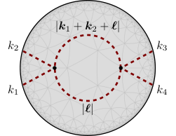
The algorithm we presented in section 3.1, and its extension in section 3.2 readily applies to loops as well. In [61], such calculations are already done in the context of cosmological wavefunctions; here, we will illustrate the algorithm in the simplest case of one loop with two vertices and use it to calculate 1 loop corrections to scalar amplitudes in AdS.2525 25 We refer the reader to [93] for analysis of similar loop diagrams of conformally coupled scalars dual to vacuum correlator instead of transition amplitudes.
The application of the algorithm in case of loops is same with that of tree level diagrams: we decompose the amplitude into sum of partial amplitudes where the expression for each partial amplitude follows from the vertex momenta inside the diagrams and the propagators going out of the diagrams. As we can see in fig. (5), there are two partial amplitudes for one loop two vertex diagram. We multiply the corresponding expressions for each subdiagram in the denominator; we listed them from outward to inward: the first value, , corresponds to the big circle, and the last ones correspond to small pink circles. In the end, the final expression takes a rather compact form in our notation: .
If we were dealing with a tree-level expression, we were done: we could simply translate from this truncated amplitude to a Witten diagram via eqn. (3.6). However, and depends on the loop amplitude and one needs to integrate it as well.
Let us illustrate this in case of loop correction to a two point function, the first diagram in fig. (4), where we are assuming interaction in AdS6.2626 26 As we saw in section , is the only case for which interaction can be calculated without additional -integrations, which we would like to avoid to give the simplest example as the illustration. In this simple case the integrand becomes
| (3.21) |
which is to be integrated over . As the integration domain is invariant under successive applications of and , which interchanges first and second term above, we can write the truncated amplitude as
| (3.22) |
which reads in spherical coordinates after the Wick rotation as
| (3.23) |
where is the volume of sphere. We can carry out the integration immediately, yielding
| (3.24) |
Clearly, this is a divergent integral. By regularizing it with a hard cut-off 2727 27 We thank Aaron Hillman for pointing out that one may need to choose dependent hard cut-off as energy scales vary with the bulk radius, and we believe that choosing should yield a more uniform energy cut-off. Nevertheless, our calculation should be fine for the purpose of illustrating the usage of algorithm with the loops., we find
| (3.25) |
In the general case of interaction in AdSd+1, we have
| (3.26) | ||||
which means under the successive applications of and under which the integration is invariant. Therefore, we have
| (3.27) |
whose integration can be immediately carried out:
| (3.28) |
Despite the term in the denominator, the integrand above is actually continuous at .
We were not able to compute the integration above for generic , however, it is quite doable once we restrict to a specific ; for example,
| (3.29) |
Note that one still needs to integrate this result with respect to and by including appropriate factors. However, we know that interaction in AdS4 is actually conformally invariant so we do not need integrations if we focus on interaction. Indeed, we can directly write the full Witten expression for the second diagram in fig. (4) as2828 28 This contradicts eqn. (3.6) because it is valid only for tree-level diagrams as we there make use of the fact that number of propagators is equal to number of vertices minus one.
| (3.30) |
4 Conclusion
In this paper, we have explored momentum space approach to computing amplitudes for scalars propagating in Anti-de Sitter space. Adopting the algorithm provided in [61] for cosmological wavefunctions, we compute both tree and loop level examples of AdS transition amplitudes.
Our momentum space formalism provides a systematic and complementary study of scalars in AdS. We are interested in using this formalism to computing higher point scalar loop amplitudes, which we leave to a future study. Likewise, this formalism can be utilized for computation of spinning loops. Unlike scalars, computing gluon and graviton loops in general dimensions is complicated, but one can get nice results if one focuses on specific dimensions [94].
There are several promising avenues for further explorations. We believe that there should be a natural polytopic interpretation to the results that we have developed, parallel to the interpretation in [61]. It is also interesting whether the weight-shifting operators developed in [50] in the context of cosmology can be generalized into our formalism, allowing us to relate spinning momentum space amplitudes to scalar momentum space amplitudes.2929 29 Such operators in positions space are constructed in [95]. Lastly, momentum space approach have been used to construct crossing symmetric basis for CFT correlators [45, 44]. Our approach could be useful in such explorations as well.
Acknowledgement
SA is supported by DOE grant no. DE-SC0020318 and Simons Foundation grant 488651. SK was supported by DRFC Discretionary Funds from Williams College.
References
- [1] J. M. Maldacena, “The Large N limit of superconformal field theories and supergravity,” Int. J. Theor. Phys. 38 (1999) 1113–1133, arXiv:hep-th/9711200 [hep-th]. [Adv. Theor. Math. Phys.2,231(1998)].
- [2] E. Witten, “Anti-de Sitter space and holography,” Adv. Theor. Math. Phys. 2 (1998) 253–291, arXiv:hep-th/9802150 [hep-th].
- [3] S. S. Gubser, I. R. Klebanov, and A. M. Polyakov, “Gauge theory correlators from noncritical string theory,” Phys. Lett. B428 (1998) 105–114, arXiv:hep-th/9802109 [hep-th].
- [4] D. Z. Freedman, S. D. Mathur, A. Matusis, and L. Rastelli, “Comments on 4 point functions in the CFT / AdS correspondence,” Phys. Lett. B452 (1999) 61–68, arXiv:hep-th/9808006 [hep-th].
- [5] H. Liu and A. A. Tseytlin, “On four point functions in the CFT / AdS correspondence,” Phys. Rev. D59 (1999) 086002, arXiv:hep-th/9807097 [hep-th].
- [6] D. Z. Freedman, S. D. Mathur, A. Matusis, and L. Rastelli, “Correlation functions in the CFT(d) / AdS(d+1) correspondence,” Nucl. Phys. B546 (1999) 96–118, arXiv:hep-th/9804058 [hep-th].
- [7] E. D’Hoker, D. Z. Freedman, and L. Rastelli, “AdS / CFT four point functions: How to succeed at z integrals without really trying,” Nucl. Phys. B562 (1999) 395–411, arXiv:hep-th/9905049 [hep-th].
- [8] E. D’Hoker, D. Z. Freedman, S. D. Mathur, A. Matusis, and L. Rastelli, “Graviton exchange and complete four point functions in the AdS / CFT correspondence,” Nucl. Phys. B562 (1999) 353–394, arXiv:hep-th/9903196 [hep-th].
- [9] J. Penedones, “Writing CFT correlation functions as AdS scattering amplitudes,” JHEP 03 (2011) 025, arXiv:1011.1485 [hep-th].
- [10] M. F. Paulos, “Towards Feynman rules for Mellin amplitudes,” JHEP 10 (2011) 074, arXiv:1107.1504 [hep-th].
- [11] G. Mack, “D-dimensional Conformal Field Theories with anomalous dimensions as Dual Resonance Models,” Bulg. J. Phys. 36 (2009) 214–226, arXiv:0909.1024 [hep-th].
- [12] A. L. Fitzpatrick, J. Kaplan, J. Penedones, S. Raju, and B. C. van Rees, “A Natural Language for AdS/CFT Correlators,” JHEP 11 (2011) 095, arXiv:1107.1499 [hep-th].
- [13] S. Kharel and G. Siopsis, “Tree-level Correlators of scalar and vector fields in AdS/CFT,” JHEP 11 (2013) 159, arXiv:1308.2515 [hep-th].
- [14] A. L. Fitzpatrick and J. Kaplan, “Analyticity and the Holographic S-Matrix,” JHEP 10 (2012) 127, arXiv:1111.6972 [hep-th].
- [15] A. L. Fitzpatrick and J. Kaplan, “Unitarity and the Holographic S-Matrix,” JHEP 10 (2012) 032, arXiv:1112.4845 [hep-th].
- [16] M. S. Costa, V. Gonalves, and J. Penedones, “Spinning AdS Propagators,” JHEP 09 (2014) 064, arXiv:1404.5625 [hep-th].
- [17] C. B. Jepsen and S. Parikh, “Recursion Relations in -adic Mellin Space,” J. Phys. A52 no. 28, (2019) 285401, arXiv:1812.09801 [hep-th].
- [18] C. B. Jepsen and S. Parikh, “-adic Mellin Amplitudes,” JHEP 04 (2019) 101, arXiv:1808.08333 [hep-th].
- [19] S. S. Gubser, C. Jepsen, and B. Trundy, “Spin in -adic AdS/CFT,” J. Phys. A52 no. 14, (2019) 144004, arXiv:1811.02538 [hep-th].
- [20] E. Hijano, P. Kraus, E. Perlmutter, and R. Snively, “Witten Diagrams Revisited: The AdS Geometry of Conformal Blocks,” JHEP 01 (2016) 146, arXiv:1508.00501 [hep-th].
- [21] E. Y. Yuan, “Simplicity in AdS Perturbative Dynamics,” arXiv:1801.07283 [hep-th].
- [22] K. Ghosh, “Polyakov-Mellin Bootstrap for AdS loops,” arXiv:1811.00504 [hep-th].
- [23] J. Liu, E. Perlmutter, V. Rosenhaus, and D. Simmons-Duffin, “-dimensional SYK, AdS Loops, and Symbols,” JHEP 03 (2019) 052, arXiv:1808.00612 [hep-th].
- [24] S. Parikh, “Holographic dual of the five-point conformal block,” arXiv:1901.01267 [hep-th].
- [25] C. B. Jepsen and S. Parikh, “Propagator identities, holographic conformal blocks, and higher-point AdS diagrams,” JHEP 10 (2019) 268, arXiv:1906.08405 [hep-th].
- [26] J. Penedones, J. A. Silva, and A. Zhiboedov, “Nonperturbative Mellin Amplitudes: Existence, Properties, Applications,” arXiv:1912.11100 [hep-th].
- [27] F. Aprile, J. Drummond, P. Heslop, and H. Paul, “One-loop amplitudes in supergravity from SYM at strong coupling,” arXiv:1912.01047 [hep-th].
- [28] D. Ponomarev, “From bulk loops to boundary large-N expansion,” arXiv:1908.03974 [hep-th].
- [29] D. Meltzer, “AdS/CFT Unitarity at Higher Loops: High-Energy String Scattering,” arXiv:1912.05580 [hep-th].
- [30] D. Meltzer, E. Perlmutter, and A. Sivaramakrishnan, “Unitarity Methods in AdS/CFT,” arXiv:1912.09521 [hep-th].
- [31] S. Caron-Huot and A.-K. Trinh, “All tree-level correlators in AdS5S5 supergravity: hidden ten-dimensional conformal symmetry,” JHEP 01 (2019) 196, arXiv:1809.09173 [hep-th].
- [32] S. Fichet, “Opacity and effective field theory in anti–de Sitter backgrounds,” Phys. Rev. D100 no. 9, (2019) 095002, arXiv:1905.05779 [hep-th].
- [33] S. Raju, “BCFW for Witten Diagrams,” Phys. Rev. Lett. 106 (2011) 091601, arXiv:1011.0780 [hep-th].
- [34] I. Mata, S. Raju, and S. Trivedi, “CMB from CFT,” JHEP 07 (2013) 015, arXiv:1211.5482 [hep-th].
- [35] S. Raju, “Four Point Functions of the Stress Tensor and Conserved Currents in AdS4/CFT3,” Phys. Rev. D85 (2012) 126008, arXiv:1201.6452 [hep-th].
- [36] S. Raju, “New Recursion Relations and a Flat Space Limit for AdS/CFT Correlators,” Phys. Rev. D85 (2012) 126009, arXiv:1201.6449 [hep-th].
- [37] S. Raju, “Recursion Relations for AdS/CFT Correlators,” Phys. Rev. D83 (2011) 126002, arXiv:1102.4724 [hep-th].
- [38] N. Arkani-Hamed and J. Maldacena, “Cosmological Collider Physics,” arXiv:1503.08043 [hep-th].
- [39] A. Bzowski, P. McFadden, and K. Skenderis, “Implications of conformal invariance in momentum space,” JHEP 03 (2014) 111, arXiv:1304.7760 [hep-th].
- [40] A. Bzowski, P. McFadden, and K. Skenderis, “Scalar 3-point functions in CFT: renormalisation, beta functions and anomalies,” JHEP 03 (2016) 066, arXiv:1510.08442 [hep-th].
- [41] A. Bzowski, P. McFadden, and K. Skenderis, “Renormalised CFT 3-point functions of scalars, currents and stress tensors,” JHEP 11 (2018) 159, arXiv:1805.12100 [hep-th].
- [42] A. Bzowski, P. McFadden, and K. Skenderis, “Evaluation of conformal integrals,” JHEP 02 (2016) 068, arXiv:1511.02357 [hep-th].
- [43] H. Isono, T. Noumi, and T. Takeuchi, “Momentum space conformal three-point functions of conserved currents and a general spinning operator,” JHEP 05 (2019) 057, arXiv:1903.01110 [hep-th].
- [44] H. Isono, T. Noumi, and G. Shiu, “Momentum space approach to crossing symmetric CFT correlators,” JHEP 07 (2018) 136, arXiv:1805.11107 [hep-th].
- [45] H. Isono, T. Noumi, and G. Shiu, “Momentum space approach to crossing symmetric CFT correlators. Part II. General spacetime dimension,” JHEP 10 (2019) 183, arXiv:1908.04572 [hep-th].
- [46] C. Corianò and M. M. Maglio, “Exact Correlators from Conformal Ward Identities in Momentum Space and the Perturbative Vertex,” Nucl. Phys. B938 (2019) 440–522, arXiv:1802.07675 [hep-th].
- [47] C. Corianò, M. M. Maglio, A. Tatullo, and D. Theofilopoulos, “Exact Correlators from Conformal Ward Identities in Momentum Space and Perturbative Realizations,” in 18th Hellenic School and Workshops on Elementary Particle Physics and Gravity (CORFU2018) Corfu, Corfu, Greece, August 31-September 28, 2018. 2019. arXiv:1904.13174 [hep-ph].
- [48] C. Corianò and M. M. Maglio, “On Some Hypergeometric Solutions of the Conformal Ward Identities of Scalar 4-point Functions in Momentum Space,” arXiv:1903.05047 [hep-th].
- [49] M. Gillioz, “Momentum-space conformal blocks on the light cone,” JHEP 10 (2018) 125, arXiv:1807.07003 [hep-th].
- [50] N. Arkani-Hamed, D. Baumann, H. Lee, and G. L. Pimentel, “The Cosmological Bootstrap: Inflationary Correlators from Symmetries and Singularities,” arXiv:1811.00024 [hep-th].
- [51] C. Corianò and M. M. Maglio, “The general 3-graviton vertex () of conformal field theories in momentum space in ,” Nucl. Phys. B937 (2018) 56–134, arXiv:1808.10221 [hep-th].
- [52] C. Corianò, L. Delle Rose, E. Mottola, and M. Serino, “Solving the Conformal Constraints for Scalar Operators in Momentum Space and the Evaluation of Feynman’s Master Integrals,” JHEP 07 (2013) 011, arXiv:1304.6944 [hep-th].
- [53] A. Bzowski, P. McFadden, and K. Skenderis, “Conformal -point functions in momentum space,” arXiv:1910.10162 [hep-th].
- [54] N. Anand, Z. U. Khandker, and M. T. Walters, “Momentum space CFT correlators for Hamiltonian truncation,” arXiv:1911.02573 [hep-th].
- [55] M. Gillioz, “Conformal 3-point functions and the Lorentzian OPE in momentum space,” arXiv:1909.00878 [hep-th].
- [56] J. A. Farrow, A. E. Lipstein, and P. McFadden, “Double copy structure of CFT correlators,” JHEP 02 (2019) 130, arXiv:1812.11129 [hep-th].
- [57] A. Lipstein and P. McFadden, “Double copy structure and the flat space limit of conformal correlators in even dimensions,” arXiv:1912.10046 [hep-th].
- [58] B. Nagaraj and D. Ponomarev, “Spinor-Helicity Formalism for Massless Fields in AdS4 II: Potentials,” arXiv:1912.07494 [hep-th].
- [59] S. Albayrak and S. Kharel, “Towards the higher point holographic momentum space amplitudes,” JHEP 02 (2019) 040, arXiv:1810.12459 [hep-th].
- [60] S. Albayrak and S. Kharel, “Towards the higher point holographic momentum space amplitudes II: Gravitons,” JHEP 12 (2019) 135, arXiv:1908.01835 [hep-th].
- [61] N. Arkani-Hamed, P. Benincasa, and A. Postnikov, “Cosmological Polytopes and the Wavefunction of the Universe,” arXiv:1709.02813 [hep-th].
- [62] S. Albayrak, C. Chowdhury, and S. Kharel, “New relation for Witten diagrams,” JHEP 10 (2019) 274, arXiv:1904.10043 [hep-th].
- [63] J. M. Maldacena, “Non-Gaussian features of primordial fluctuations in single field inflationary models,” JHEP 05 (2003) 013, arXiv:astro-ph/0210603 [astro-ph].
- [64] A. Ghosh, N. Kundu, S. Raju, and S. P. Trivedi, “Conformal Invariance and the Four Point Scalar Correlator in Slow-Roll Inflation,” JHEP 07 (2014) 011, arXiv:1401.1426 [hep-th].
- [65] P. McFadden and K. Skenderis, “Holography for Cosmology,” Phys. Rev. D81 (2010) 021301, arXiv:0907.5542 [hep-th].
- [66] X. Chen and Y. Wang, “Quasi-Single Field Inflation and Non-Gaussianities,” JCAP 1004 (2010) 027, arXiv:0911.3380 [hep-th].
- [67] J. M. Maldacena and G. L. Pimentel, “On graviton non-Gaussianities during inflation,” JHEP 09 (2011) 045, arXiv:1104.2846 [hep-th].
- [68] D. Baumann and D. Green, “Signatures of Supersymmetry from the Early Universe,” Phys. Rev. D85 (2012) 103520, arXiv:1109.0292 [hep-th].
- [69] V. Assassi, D. Baumann, and D. Green, “On Soft Limits of Inflationary Correlation Functions,” JCAP 1211 (2012) 047, arXiv:1204.4207 [hep-th].
- [70] X. Chen and Y. Wang, “Quasi-Single Field Inflation with Large Mass,” JCAP 1209 (2012) 021, arXiv:1205.0160 [hep-th].
- [71] V. Assassi, D. Baumann, D. Green, and L. McAllister, “Planck-Suppressed Operators,” JCAP 1401 (2014) 033, arXiv:1304.5226 [hep-th].
- [72] H. Lee, D. Baumann, and G. L. Pimentel, “Non-Gaussianity as a Particle Detector,” JHEP 12 (2016) 040, arXiv:1607.03735 [hep-th].
- [73] H. An, M. McAneny, A. K. Ridgway, and M. B. Wise, “Quasi Single Field Inflation in the non-perturbative regime,” JHEP 06 (2018) 105, arXiv:1706.09971 [hep-ph].
- [74] A. Kehagias and A. Riotto, “On the Inflationary Perturbations of Massive Higher-Spin Fields,” JCAP 1707 no. 07, (2017) 046, arXiv:1705.05834 [hep-th].
- [75] S. Kumar and R. Sundrum, “Heavy-Lifting of Gauge Theories By Cosmic Inflation,” JHEP 05 (2018) 011, arXiv:1711.03988 [hep-ph].
- [76] D. Baumann, G. Goon, H. Lee, and G. L. Pimentel, “Partially Massless Fields During Inflation,” JHEP 04 (2018) 140, arXiv:1712.06624 [hep-th].
- [77] G. Franciolini, A. Kehagias, and A. Riotto, “Imprints of Spinning Particles on Primordial Cosmological Perturbations,” JCAP 1802 no. 02, (2018) 023, arXiv:1712.06626 [hep-th].
- [78] G. Goon, K. Hinterbichler, A. Joyce, and M. Trodden, “Shapes of gravity: Tensor non-Gaussianity and massive spin-2 fields,” arXiv:1812.07571 [hep-th].
- [79] D. Anninos, V. De Luca, G. Franciolini, A. Kehagias, and A. Riotto, “Cosmological Shapes of Higher-Spin Gravity,” JCAP 1904 no. 04, (2019) 045, arXiv:1902.01251 [hep-th].
- [80] S. Pi and M. Sasaki, “Curvature Perturbation Spectrum in Two-field Inflation with a Turning Trajectory,” JCAP 1210 (2012) 051, arXiv:1205.0161 [hep-th].
- [81] J.-O. Gong, S. Pi, and M. Sasaki, “Equilateral non-Gaussianity from heavy fields,” JCAP 1311 (2013) 043, arXiv:1306.3691 [hep-th].
- [82] C. Sleight, “A Mellin Space Approach to Cosmological Correlators,” arXiv:1906.12302 [hep-th].
- [83] C. Sleight and M. Taronna, “Bootstrapping Inflationary Correlators in Mellin Space,” arXiv:1907.01143 [hep-th].
- [84] A. Hillman, “Symbol Recursion for the dS Wave Function,” arXiv:1912.09450 [hep-th].
- [85] S. Sonego and V. Faraoni, “Coupling to the curvature for a scalar field from the equivalence principle,” Class. Quant. Grav. 10 (1993) 1185–1187.
- [86] N. D. Birrell and P. C. W. Davies, Quantum Fields in Curved Space. Cambridge Monographs on Mathematical Physics. Cambridge Univ. Press, Cambridge, UK, 1984. http://www.cambridge.org/mw/academic/subjects/physics/theoretical-physics-and-mathematical-physics/quantum-fields-curved-space?format=PB.
- [87] G. W. Gibbons and S. W. Hawking, “Action Integrals and Partition Functions in Quantum Gravity,” Phys. Rev. D15 (1977) 2752–2756.
- [88] A. Guarnizo, L. Castaneda, and J. M. Tejeiro, “Boundary Term in Metric f(R) Gravity: Field Equations in the Metric Formalism,” Gen. Rel. Grav. 42 (2010) 2713–2728, arXiv:1002.0617 [gr-qc].
- [89] S. Nojiri and S. D. Odintsov, “Brane world cosmology in higher derivative gravity or warped compactification in the next-to-leading order of AdS / CFT correspondence,” JHEP 07 (2000) 049, arXiv:hep-th/0006232 [hep-th].
- [90] D. Carmi, “Loops in AdS: From the Spectral Representation to Position Space,” arXiv:1910.14340 [hep-th].
- [91] D. Baumann, C. Duaso Pueyo, A. Joyce, H. Lee, and G. L. Pimentel, “The Cosmological Bootstrap: Weight-Shifting Operators and Scalar Seeds,” arXiv:1910.14051 [hep-th].
- [92] V. Faraoni, “Conformally coupled inflation,” Galaxies 1 no. 2, (2013) 96–106.
- [93] S. Giombi, C. Sleight, and M. Taronna, “Spinning AdS Loop Diagrams: Two Point Functions,” JHEP 06 (2018) 030, arXiv:1708.08404 [hep-th].
- [94] S. Albayrak and S. Kharel, “On spinning loop amplitudes in Anti-de Sitter space,” arXiv:2006.12540 [hep-th].
- [95] M. S. Costa and T. Hansen, “AdS Weight Shifting Operators,” arXiv:1805.01492 [hep-th].