FlexiBO: A Decoupled Cost-Aware Multi-Objective Optimization Approach for Deep Neural Networks

Md Shahriar Iqbal miqbal@email.sc.edu Affiliation: University of South Carolina, Columbia, SC, USA Jianhai Su suj@email.sc.edu Affiliation: University of South Carolina, Columbia, SC, USA Lars Kotthoff larsko@uwyo.edu Affiliation: University of Wyoming, Laramie, WY, USA Pooyan Jamshidi pjamshid@cse.sc.edu Affiliation: University of South Carolina, Columbia, SC, USA

Abstract

The design of machine learning systems often requires trading off different objectives, for example, prediction error and energy consumption for deep neural networks (DNNs). Typically, no single design performs well in all objectives; therefore, finding Pareto-optimal designs is of interest. The search for Pareto-optimal designs involves evaluating designs in an iterative process, and the measurements are used to evaluate an acquisition function that guides the search process. However, measuring different objectives incurs different costs. For example, the cost of measuring the prediction error of DNNs is orders of magnitude higher than that of measuring the energy consumption of a pre-trained DNN as it requires re-training the DNN. Current state-of-the-art methods do not consider this difference in objective evaluation cost, potentially incurring expensive evaluations of objective functions in the optimization process. In this paper, we develop a novel decoupled and cost-aware multi-objective optimization algorithm, we call Flexible Multi-Objective Bayesian Optimization (FlexiBO) to address this issue. For evaluating each design, FlexiBO selects the objective with higher relative gain by weighting the improvement of the hypervolume of the Pareto region with the measurement cost of each objective. This strategy, therefore, balances the expense of collecting new information with the knowledge gained through objective evaluations, preventing FlexiBO from performing expensive measurements for little to no gain. We evaluate FlexiBO on seven state-of-the-art DNNs for image recognition, natural language processing (NLP), and speech-to-text translation. Our results indicate that, given the same total experimental budget, FlexiBO discovers designs with 4.8 $\%$ to 12.4 $\%$ lower hypervolume error than the best method in state-of-the-art multi-objective optimization.

1 Introduction

(a) a

(b) b

Figure 1: (a) The system stack of a DNN, composed of six components. (b) Performance variation of several hundred designs for an image recognition DNN system, SqueezeNet, deployed on resource-constrained Nvidia Jetson TX2 hardware while performing inference on 5,000 test images. We observe that there is substantial variation for each performance objective across different designs, i.e., prediction error varies 3

\times

, energy consumption varies 4

\times

. Designs marked with blue rectangles optimally trade off both objectives.

Recent developments of deep neural networks (DNNs) have sparked a growing demand for pushing the deployment of artificial intelligence applications from the cloud to a wide variety of edge and IoT devices. As these devices are closer to data and information generation sources, they provide better user experience e.g., latency and throughput sensitivity, security etc. Compared to datacenters, the edge devices are more resource-constrained and may not be even able to host these compute expensive DNN models. Therefore, designing energy-efficient DNNs is critical for successful deployment of DNNs to these devices with limited resources. On one hand, high inference error often leads to application failures (?, ?), but on the other hand, it is essential to reduce the number of computation cycles and/or memory footprints of DNNs to conserve energy (?). In addition to DNN models, a number of components in the DNN system stack (shown in Figure 1a) must work together for the seamless deployment of energy-efficient DNNs without compromising inference accuracy (?, ?).

There exist 100s if not 1000s of design options from each component across the DNN system stack that impact the computational and memory requirements of DNNs and make them difficult to effectively deploy. One of the key challenges in designing an optimal DNN system is to efficiently explore the vast design space, with non-trivial interactions of options from different components across the system stack, e.g., CPU frequency, GPU frequency, number of epochs, etc. Additionally, there is usually no single design that performs well for all performance objectives (see e.g. Figure 1b). Therefore, we need to identify designs that provide optimal trade-offs – Pareto optimal designs.

Method	Method Type	Search Strategy	Evaluation Strategy	Cost Awareness
NEMO ( ?)		NAS	Gradient Based	Coupled	✗
DPP-NET (?)	NAS	Gradient Based	Coupled	✗
HR (?)	NAS	Gradient Based	Coupled	✗
ParEGO (?)	MOBO	Random Scalarization	Coupled	✗
SMSego (?)	MOBO	Hypervoume Improvement	Coupled	✗
PAL (?)	MOBO	Predictive Uncertainty	Coupled	✗
MESMO (?)	MOBO	Output Space Entropy	Coupled	✗
PESMO (?)	MOBO	Input Space Entropy	Coupled	✗
PESMO-DEC (?)	MOBO	Input Space Entropy	De-coupled	✗
CA-MOBO (?)	MOBO	Chebyshev Scalarization	Coupled	✓
FlexiBO	MOBO	Volume of the Pareto region	De-coupled	✓

Figure 2: Comparison of FlexiBO to related state-of-the-art methods that can be used to identify Pareto optimal solutions.

Previous work has focused on neural architecture search (NAS) techniques that can efficiently locate Pareto optimal designs. NAS approaches like Nemo (?), hierarchical representations (HR) (?), and DPP-NET (?) can be categorized according to three different criteria: (i) the Search Space, (ii) the Optimization Method, and (iii) the Candidate Evaluation Method. Unfortunately, the effectiveness of NAS approaches largely depends on selecting a quality search space to reduce the complexity of search that requires significant prior knowledge that is difficult to find in practice, which also indicates that they are not suitable in different platforms. Much recent work has focused on multi-objective Bayesian optimization (MOBO) approaches like ParEGO (?), SMSego (?), PAL (?), PESMO (?), MESMO (?), MESMOC (?) etc. to find the Pareto optimal designs that can used for hyperparameter tuning. MOBO approaches iteratively use the uncertainty captured by a probabilistic model (also known as the surrogate model, an approximation that is much faster and cheaper to evaluate than the complex unknown function to be optimized) of the process to be optimized to compute the values of an acquisition function. The optimum of the acquisition function provides an effective heuristic for identifying a promising design for which to evaluate the objectives. Nevertheless, there are limitations to these MOBO approaches. For instance, scalarization-based approaches (ParEGO) tend to suffer from sub-optimality, algorithms to optimize hypervolume based acquisition function (SMSego) scale poorly when the input dimensionality increases, methods that rely on entropy-based acquisition functions (PESMO, MESMO, MESMOC) are computationally expensive, and PAL is simple to design but also requires a lot of computation at each iteration.

Furthermore, most of these methods are cost unaware and consider the objective evaluation costs to be uniform. In practice, the cost of objective evaluations can be non-uniform e.g., optimizing prediction error in DNN systems is much more expensive than making predictions with a pre-trained DNN with different deployment system design options as that involves re-training the whole DNN. Besides, existing approaches use a coupled evaluation strategy to evaluate the design selected by the optimizers across all objectives, at each iteration. Iterative optimizers must balance exploiting the knowledge gained from the evaluations with exploring regions in the search space where the landscape is unknown and might hold better designs. This balance is particularly acute with limited experimental budgets, e.g., DNNs deployed on production or resource-constrained devices that can inhibit efficient finding of Pareto optimal designs. Recently, CA-MOBO (?) proposed a cost-aware approach to identify the Pareto optimal designs by avoiding the designs with high evaluation costs in the design space. However, this can lead to aggressive exploitation behavior and generate sub-optimal designs. PESMO-DEC introduces a decoupled evaluation strategy where only a subset of objectives at any given location is evaluated. The decoupled evaluation provides significant improvements over a coupled evaluation, particularly when the experimentation budget is limited. However, selecting designs to evaluate without considering non-uniform evaluation costs can potentially lead to inefficient utilization of resources.

To address these limitations, we propose the cost-aware decoupled MOBO approach FlexiBO, which explicitly considers non-uniform objective evaluation costs and evaluates expensive objectives only if the gain of information is worth it. FlexiBO extends the concepts of the state-of-the-art active learning algorithm PAL (?) and PESMO-DEC (?). To our knowledge, this is the first approach to propose a cost-aware decoupled evaluation strategy for MOBO. To formalize the notion of non-uniform evaluation costs of objectives, we define objective evaluation cost in terms of computation time. Our acquisition function incorporates the uncertainty of the surrogate model’s predictions and objective evaluation costs to balance exploration and exploitation and iteratively improve the quality of the Pareto optimal design space, also known as the Pareto region. It selects the objectives across which the design will be evaluated in addition to selecting the next design to evaluate. Consequently, we explicitly trade off the additional information obtained through an evaluation with the cost of obtaining it, ensuring that we do not perform costly evaluations for little potential gain. By avoiding costly evaluations, we improve the efficiency of the search for Pareto optimal designs. We demonstrate FlexiBO’s promise through a comprehensive experimental evaluation on a range of different benchmarks. While we focus on DNNs, our proposed approach is general and can be extended to other applications.

1.1 Contributions

In summary, our contributions are as follows.

$\blacktriangleright$

We propose FlexiBO: a cost-aware approach for multi-objective Bayesian optimization that selects a design and an objective for evaluation. It allows to trade off the additional information gained through an evaluation and the cost being incurred as a result of the evaluation (Section 5).
$\blacktriangleright$

We comprehensively evaluate FlexiBO on seven DNN architectures from three different domains and compare its performance to ParEGO (?), SMSego (?), PAL (?), and PESMO,PESMO-DEC (?), and CA-MOBO (?). (Section 6). The dataset and scripts to reproduce our findings are available at https://github.com/softsys4ai/FlexiBO.

(a) a

(b) b

(d) d

Figure 3: (a) Cost-unaware coupled approaches waste resources by evaluating designs with higher evaluation costs. (b) Cost-aware coupled approaches can suffer poor performance if the Pareto optimal designs can only be found by evaluating objectives with high evaluation cost. (c) Cost-unaware decoupled approaches can invest a lot of resources in evaluating designs with low quality (high prediction error and high energy consumption) and do not perform well across both objectives. (d) Cost-aware decoupled approaches find designs with better quality compared to other approaches. Yellow stars indicates the location of Pareto optimal designs. The color indicates the evaluation cost (log wall-clock time) of a particular design.

2 Motivation

In this section, we discuss our motivation to propose a cost-aware and decoupled evaluation strategy. Based on the cost distribution assumptions and evaluation strategy, existing MOBO techniques can be subdivided into the following categories: (I) cost-unaware coupled, (II) cost-aware coupled, and (III) cost-unaware decoupled approaches. Unlike cost-unaware approaches, cost-aware approaches assume the cost of evaluating different objectives is non-uniform. Decoupled approaches consider only a subset of objectives for evaluation at each iteration in the Bayesian optimization loop whereas coupled approaches evaluate all objectives. To show the clear advantage of our proposed cost-aware decoupled approach (to our knowledge, a gap in the MOBO literature that has not been addressed yet), we performed a sandbox experiment to optimize the prediction error and energy consumption of the image recognition DNN system SqueezeNet for the CIFAR-10 dataset deployed on an Nvidia JETSON TX2 device for inference on 5,000 test images. We use 8 Nvidia Tesla K80 GPUs deployed on Google cloud for training with 45,000 training images. We tuned a small subset of design options from different layers of the system stack – CPU frequency and GPU frequency from the hardware layer, swappiness from the operating system layer, memory growth from the model compiler layer, and filter size, number of filters, and number of epochs from the DNN model layer. We use PAL as a cost-unaware coupled approach, CA-MOBO as a cost-aware coupled approach, PESMO-DEC as a cost-unaware decoupled approach, and FlexiBO as a cost-aware decoupled approach.

Cost-unaware coupled approaches are not sample (design) efficient for budget-constrained applications as they do not make the best utilization of resources by evaluating the selected designs across all objectives even for little or no gain. Figure 3a shows that most of the designs selected by the cost-unaware coupled approach are not close to the Pareto front and are concentrated in regions with high evaluation costs. It also has poor coverage of the objective space.

(a) a

(b) b

Figure 4: Contour curves for (a) prediction error and (b) energy consumption of SqueezeNet by varying CPU Frequency and Number of Filters while keeping the other design options fixed. Decoupled unaware approaches perform poorly when objectives with different costs have the same complexity (both non-linear).

Cost-aware coupled approaches consider different evaluation costs for different designs. As such approaches only evaluate cheap designs, good parts of the search space may be missed. Figure 3b shows that the cost-aware coupled strategy focuses on the cheap regions of the search space here and misses Pareto’s optimal designs in expensive regions.

Cost-unaware decoupled approaches evaluate the more complex objectives a higher number of times than the less complex objectives. However, Figure 4a and Figure 4b show that both the objectives (e.g., prediction error and energy consumption) have the same complexity. Cost unaware approaches are not particularly effective in such cases and produce suboptimal results as shown in Figure 3c. This occurs as a result of them not making the best use of resources by evaluating a large number of low-quality designs (high prediction error and high energy consumption) for little information gain.

Cost-aware decoupled approaches evaluate designs in any region if the information gain is large enough given the objective evaluation cost. In Figure 3d, we observe that our cost-aware decoupled approach performs better than the other approaches and identifies more points on the Pareto front.

3 Related Work

We now discuss different directions of related work for multi-objective optimization.

Hardware-aware optimization of DNNs.

One of the largest difficulties in producing energy-efficient DNNs is the disconnect between the platform where the DNN is designed, developed, and tested, and the platform where it will eventually be deployed and the energy it consumes there (?, ?, ?, ?, ?, ?, ?). Therefore, hardware-aware multi-objective optimization approaches have been introduced (?, ?, ?, ?, ?) that enable automatic optimization of DNNs in the joint space of architectures, hyperparameters, and even the computer system stack (?, ?, ?, ?). Like these approaches, FlexiBO enables efficient multi-objective optimization in such joint configuration spaces. Multi-objective neural architecture search (NAS) (?, ?, ?) aims to optimize accuracy and limit resource consumption, for example by limiting the search space (?). Several approaches characterize runtime, power, and the energy consumption of DNNs via analytical models, e.g., Paleo (?), NeuralPower (?), Eyeriss (?), and Delight (?). However, they either rely on proxies like inference time for energy consumption or extrapolate energy values from energy-per-operation tables. They therefore cannot be used across different deployment platforms.

Multi-Objective Optimization with Different Acquisition Functions.

There is a large body of research that identifies the complete Pareto front using entropy-based acquisition functions. For example, MESMO (?, ?), MESMOC (?), and PESMO (?) determine the Pareto front by reducing posterior entropy. SMSego uses the maximum hypervolume improvement acquisition function to choose the next sample (?). Different gradient-based multi-objective optimization algorithms have been proposed to optimize objectives more efficiently (?, ?). These methods were extended to use stochastic gradient descent (?, ?). Active learning approaches have been proposed to approximate the surface of the Pareto front (?) through the use of acquisition functions such as expected hypervolume improvement (?) and sequential uncertainty reduction (?). Contemporary active learning approaches like PAL and $\epsilon$ -PAL tend to approximate the Pareto front (?, ?) using the maximum diagonal of the uncertainties in the objective space as the acquisition function. However, these methods do not take into account the varying costs of the evaluations of the objective functions and are expensive.

Multi-Objective Optimization With Preferences.

Some methods use preferences in multi-objective optimization with evolutionary methods (?, ?, ?); although these methods enable the user to guide the exploration of the design space of systems (?), they are not sample-efficient, which is essential for optimizing highly-configurable systems (?, ?, ?, ?, ?), particularly for very large configuration spaces (?). Recently, methods that use surrogate models for optimization with preferences have been proposed (?, ?). These methods require the user to manually specify a preference though and are not cost-efficient.

Multi-Objective Optimization With Scalarizations.

Different multi-objective optimization methods have been developed that use scalarizations to combine multiple objectives into a single one such that optimal solutions correspond to Pareto-optimal solutions. Examples include ParEGO, which uses random scalarizations (?), weighted product methods (?), and utility functions (?, ?, ?, ?). A major disadvantage of the scalarization approach is that without further assumptions (e.g., convexity) on the objectives, not all Pareto optimal solutions can be recovered. Therefore, solutions obtained by scalarization approaches tend to be sub-optimal.

Cost-Aware Multi-Objective Optimization Approaches.

Recently, different cost-aware methods (?, ?) have been proposed that incorporate the evaluation costs of objectives into account. They assign costs to designs in the design space and attempt to identity an optimal Pareto front by avoiding the costly designs; thereby selecting cheap designs for evaluation. These methods are either orthogonal or complimentary to our approach. FlexiBO is a decoupled approach where we trade off the evaluation cost of an objective with the amount of information that can be gained.

4 Background and Definitions

In this section, we review MOBO and Pareto optimality and introduce the terminology and notation used in the rest of the paper. Table 7 in the appendix lists the symbols and their descriptions used throughout the paper.

Bayesian Optimization.

Bayesian Optimization (BO) is an efficient framework to solve global optimization problems using black-box evaluations of expensive objective functions (?). Let $\mathfrak{X}\subset\mathbb{R}^{d},$ where $d\in\mathbb{N}$ , be a finite design space. For single-objective Bayesian optimization (SOBO), we are given a real-valued objective function $f:\mathfrak{X}\rightarrow\mathbb{R}$ , which can be evaluated at each design $\bm{x}\in\mathfrak{X}$ to produce an evaluation $y=f(\bm{x})$ . Each evaluation of $\bm{x}$ is expensive in terms of the consumed resources. The main goal is to find a design $\bm{x}^{*}\in\mathfrak{X}$ that optimizes $f$ by performing a limited number of function evaluations. BO approaches use a cheap surrogate model learned from training data obtained using past function evaluations. They intelligently select designs for evaluation by searching over the surrogate model, trading off exploration and exploitation to quickly direct the search towards an optimal design.

Acquisition Function.

This is used to score the utility of evaluating a candidate design $\bm{x}\in\mathfrak{X}$ based on the statistical model. Some popular acquisition functions in the SOBO literature include expected improvement (EI) (?), upper confidence bound (UCB) (?), predictive entropy search (PES) (?), and max-value entropy search (MES) (?).

Figure 5: The design space

\mathfrak{X}

is mapped to the objective space

\mathfrak{F}

for

n=2

. The objective space is showing examples uncertainty regions

R(\bm{x})

for different designs

\bm{x}

MOBO.

In MOBO, the aim is to find a set of designs that simultaneously optimizes $n$ possibly conflicting objective functions $\bm{f}=f_{1},\dots,f_{n}$ , where $n\geq 2$ and ${f_{i}}:\mathfrak{X}\rightarrow\mathbb{R}$ for $1\leq i\leq n$ . Each evaluation of a design $\bm{x}\in\mathfrak{X}$ produces a vector of objective values $\bm{y}=(y_{1},...,y_{n})$ , where $y_{i}=f_{i}(\bm{x})$ for $1\leq i\leq n$ .

Pareto-Optimality.

It is generally not possible to find a design that optimizes each objective equally, but instead, there is a trade-off between them. Pareto optimal designs represent the best compromises across all objectives. In the context of maximization, a design $\bm{x}$ is said to dominate another design $\bm{x}^{\prime}$ , formally, $\bm{x}\succeq\bm{x}^{\prime}$ if $f_{i}(\bm{x})\geq f_{i}(\bm{x}^{\prime})$ for $1\leq i\leq n$ . A design $\bm{x}\in\mathfrak{X}$ is called Pareto-optimal if it is not dominated by any other designs $\bm{x}^{\prime}\in\mathfrak{X}$ , where $\bm{x}\neq\bm{x}^{\prime}$ . The set of designs $\mathfrak{X}^{*}$ is called the optimal Pareto set and a hyperplane¹¹ 1 A subspace of the design space whose dimension is one less than the design space. passing through the corresponding set of function values $\mathfrak{F}^{*}$ is called the Pareto front.

Surrogate Model

Surrogate models $\mathfrak{M_{i}}$ for $1\leq i\leq n$ are used to approximate the function to optimize, which is usually computationally expensive to evaluate and not available in closed form. Surrogate models are trained with evaluations of a small subset of the design space $\mathfrak{X}$ and are used to predict the objective functions value using $\hat{f}(\bm{x})=\bm{\mu}(\bm{x})$ with estimation uncertainty $\bm{\sigma}(\bm{x})$ for each design $\bm{x}$ . The uncertainty region $R(\bm{x})$ of a design $\bm{x}$ is defined as a hyper-rectangle of the width of the confidence region using $\bm{\mu}(\bm{x})$ and $\bm{\sigma}(\bm{x})$ (formally defined later).

Figure 6: The objective space is showing examples of Pareto fronts

\mathfrak{F}_{pess}

and

\mathfrak{F}_{opt}

passing through a subset of non-dominated designs. Here, non-dominated designs are shown in gray and dominated designs are shown in black.

Optimistic and Pessimistic Pareto front.

Each design $\bm{x}$ in the design space $\mathfrak{X}$ is assigned an uncertainty region $R(\bm{x})$ using the predictions of the objective functions $\bm{f}$ from the surrogate models $\mathfrak{M}$ . Figure 5 shows an example of uncertainty region of a design and its maximum value $\max(R(\bm{x}))$ and minimum value $\min(R(\bm{x}))$ for $n=2$ objectives. The maximum value of the uncertainty region $\max(R(\bm{x}))$ and minimum value of the uncertainty region $\min(R(\bm{x}))$ of a design $\bm{x}$ are regarded as the optimistic and pessimistic value of $\bm{x}$ , respectively. A hyperplane passing through the non-dominated optimistic values of $\bm{x}$ is considered the optimistic Pareto front $\mathfrak{F}_{opt}$ . Similarly, a pessimistic Pareto front $\mathfrak{F}_{pess}$ is constructed by a hyperplane passing through the pessimistic values of $\bm{x}$ .

Pareto Region.

The region bounded by the optimistic Pareto front $\mathfrak{F}_{opt}$ and pessimistic Pareto front $\mathfrak{F_{pess}}$ is defined as the Pareto region $P_{R}$ (shown as the blue shaded region in Figure 6).

Objective evaluation cost.

Objective evaluation cost $\theta_{i}(\bm{x})$ of a design $\bm{x}$ is the computational effort required to evaluate design $\bm{x}$ for an objective $f_{i}$ .

5 FlexiBO: Flexible Multi-Objective Bayesian Optimization

In this section, we explain the technical details of our proposed Flexible Multi-Objective Bayesian Optimization (FlexiBO) algorithm. FlexiBO aims to identify the optimal Pareto front $\mathfrak{F}^{*}$ by evaluating a small subset of designs in the design space $\mathfrak{X}$ that uses a cost-aware acquisition function to incorporate the evaluation costs of each objective in the standard Bayesian optimization framework. Given the same budget $\theta_{T}$ , the cost-awareness of the acquisition function enables FlexiBO to sample the search space more efficiently compared to other state-of-the-art approaches.

5.1 Algorithm Design

FlexiBO is an active learning algorithm that selects a sequence of designs $(\bm{x}_{1},...,\bm{x}_{T})$ in the design space $\mathfrak{X}$ for evaluation to determine the Pareto-optimal designs; the designs classified as Pareto-optimal are then returned as the prediction $\mathfrak{\hat{F}}^{*}$ for $\mathfrak{F}^{*}$ . Rather than evaluating each design $\bm{x}$ against all objectives $f_{i}$ for $1\leq i\leq n$ , our cost-aware approach iteratively evaluates a selected design $\bm{x}$ only across the most informative objective. FlexiBO evaluates a design $\bm{x}$ across an objective $f_{i}$ if the change in hypervolume of the Pareto region is large enough compared to the objective evaluation cost $\theta_{i}$ . This allows FlexiBO to avoid expensive measurements for little or no change in hypervolume and to only evaluate across an objective when the change in hypervolume is worthy compared to the evaluation cost. Formally, FlexiBO is a cost-aware multi-objective optimization approach that iteratively and adaptively selects a sequence of designs and objectives $((\bm{x}_{1},f_{1,i}),...,(\bm{x}_{T},f_{T,i}))$ for $1\leq i\leq n$ across which the selected designs are evaluated to predict the Pareto front $\mathfrak{\hat{F}}^{*}$ .

We then fit a separate surrogate model $\mathfrak{M_{i}}$ for each objective function $f_{i}$ for $1\leq i\leq n$ . We select m designs set $\mathfrak{X_{m}}$ from the design space $\mathfrak{X}$ using Monte-Carlo sampling (?). The objective values of a design $\bm{x}$ that has not been evaluated across any objective are estimated by $\bm{\hat{f}}(\bm{x})=\bm{\mu}(\bm{x})=(\mu_{1}(\bm{x}),\dots,\mu_{n}(\bm{x}))$ , and the associated uncertainty is estimated by $\bm{\sigma}(\bm{x})=(\sigma_{1}(\bm{x}),\dots,\sigma_{n}(\bm{x}))$ . If a design $\bm{x}$ is evaluated across an objective $f_{i}$ , the associated uncertainty is zero against $f_{i}$ . At each iteration $t$ , we use the $\bm{\mu}_{t}(\bm{x})$ and $\bm{\sigma}_{t}(\bm{x})$ values to determine the uncertainty region $R_{t}(\bm{x})$ for each design $\bm{x}\in\mathfrak{X_{m}}$ . We define the uncertainty region associated with a prediction of the surrogate model as follows:

R_{t}(\bm{x})=\{\bm{y}:\bm{\mu}_{t}(\bm{x})-\sqrt{\beta_{t}}\bm{\sigma}_{t}(\bm{x})\leq\bm{y}\leq\bm{\mu}_{t}(\bm{x})+\sqrt{\beta_{t}}\bm{\sigma}_{t}(\bm{x})\},

(1)

where $\beta_{t}$ is a scaling parameter that controls the exploration-exploitation trade-off. Similar to PAL (?, ?), we use $\beta_{t}=2/9\log(n|\mathfrak{X_{m}}|\pi^{2}t^{2}/{6\delta})$ for $\delta\in(0,1)$ .The dimension of $R_{t}(\bm{x})$ depends on the number of objectives $n$ . Later, we exploit the information about the uncertainty regions to determine the non-dominated designs set $\mathfrak{U}$ . We then use the optimistic and pessimistic values of the non-dominated designs in $\mathfrak{U}$ to build the optimistic Pareto front $\mathfrak{F}_{opt}$ and pessimistic Pareto front

We now employ our cost-aware acquisition function, which makes use of an information gain based on objective space entropy. Being cost-aware, our proposed acquisition function $\alpha_{t,i}(\bm{x})$ considers the evaluation cost $\theta_{t,i}$ across each objective $f_{i}$ :

$\displaystyle\alpha_{t,i}(\bm{x})$	$\displaystyle=\frac{\Delta V(\{\bm{x},f_{t,i}(\bm{x})\},\mathfrak{\hat{F}}^{}\|\mathfrak{X_{m}}^{})}{\theta_{t,i}}$	(2)
	$\displaystyle=\frac{V(P_{R}\|\mathfrak{\hat{F}}^{})-V\left(P_{R}\|\mathfrak{\hat{F}}^{}_{R_{t,i}(\bm{x})=\bm{\mu}_{t,i}(\bm{x})}\right)}{\theta_{t,i}}$	(3)
	$\displaystyle=\frac{\Delta{V_{t,i}}}{{\theta_{t,i}}}$	(4)

Here, $\alpha_{t,i}(\bm{x})$ computes the amount of information that can be gained per cost for a design $\bm{x}$ to be evaluated for an objective $f_{i}$ . In Equation 3, we compute the gain of information as the change of volume of the Pareto region if the Pareto front $\mathfrak{\hat{F}}^{*}=\mathfrak{F}_{opt}\cup\mathfrak{F}_{pess}$ is updated by setting the uncertainty values $R_{t,i}(\bm{x})$ of $\bm{x}$ to its mean $\mu_{t,i}(\bm{x})$ for the corresponding designs in $\mathcal{X}_{m}^{*}$ . Our acquisition function computes the change of volume $\Delta V_{t,i}$ of the Pareto region $P_{R}$ across each objective $f_{i}$ to judiciously determine the gain of information that would be achieved if design $\bm{x}$ is evaluated for $f_{i}$ . We select a design $\bm{x}_{t}$ and an objective $f_{t,i}$ using the following:

\displaystyle\bm{x}_{t},f_{t,i}=\text{argmax}_{\bm{x}\in\mathcal{X}_{m}^{*}\ \text{for each}\ f_{i}}\ \alpha_{t,i}(\bm{x})

(5)

Here, we identify the most promising design for an objective function that gains the most information given the cost of evaluating it. Finally, we update the surrogate model $\mathcal{M}_{i}$ corresponding to the chosen objective function $f_{i}$ by incorporating the newly-evaluated design and objective value. We stop when the maximum budget $\theta_{T}$ is exhausted or the maximum change of volume of the Pareto region becomes zero (indicating that all designs in the Pareto region have been evaluated for each objective ), whichever occurs earlier. Finally, we return the Pareto front obtained. Every iteration $t$ consists of three stages: (1) modeling, (2) construction of the Pareto region, and (3) sampling. To initialize FlexiBO, we evaluate $N_{0}$ samples for each objective $f_{i}$ to and populate corresponding evaluated designs set $S_{i}$ for $1\leq i\leq n$ . We also determine the average computational effort $\theta_{i}$ for each objective $f_{i}$ before proceeding to the iterative procedure. We outline the pseudocode for the FlexiBO implementation in Algorithm 1.

Figure 7: Example showing pruning of non-dominated points to construct

\mathfrak{F}_{opt}

and

\mathfrak{F}_{pess}

Input: design space

\mathfrak{X}

; maximum budget

\theta_{T}

; number of initial designs

N_{0}

;

Initialization 1

S_{i}

= Evaluate

N_{0}

designs for each objective

f_{i}

Determine average computational effort

\theta_{i}=(\sum_{t=1}^{N_{0}}\theta_{t,i})/N_{0}

for each

f_{i}

t

N_{0}

and

\theta=0

while $\theta\leq\theta_{T}$ do 5

Modeling 6

Train surrogate models

\mathfrak{M}_{t,i}

using corresponding evaluated designs set

S_{i}

for

f_{i}

Obtain

\bm{\mu}_{t}(\bm{x})=(\mu_{t,i}(\bm{x}))_{1\leq i\leq n}

and

\bm{\sigma}_{t}(\bm{x})=(\sigma_{t,i}(\bm{x}))_{1\leq i\leq n}

using

(\mathfrak{M}_{t,i})_{1\leq i\leq n}

for all

\bm{x}\in\mathfrak{X_{m}}

. 8

Compute uncertainty region

R_{t}(\bm{x})

of each design

\bm{x}\in\mathfrak{X_{m}}

using Equation 1 9

Pareto region construction 10

\mathfrak{U}=\varnothing

for all $\bm{x}\in\mathfrak{X_{m}}$ do 12

if no $\bm{x}\neq\bm{x}^{\prime}$ for $\bm{x}^{\prime}\in\mathfrak{X_{m}}$ exists such that $\min(R_{t}(\bm{x}))\succeq\max(R_{t}(\bm{x}^{\prime}))$ then 13

\mathfrak{U}=\mathfrak{U}\cup\{\bm{x}\}

Identify optimistic Pareto front

\mathfrak{F}_{opt}

and pessimistic Pareto front

\mathfrak{F}_{pess}

using

\mathfrak{U}

and

R_{t}(\bm{x})

with Equation 7, Equation 8, and Equation 9 15

Sampling 16

Compute acquisition function

\alpha_{t,i}(\bm{x})

across each objective

f_{i}

using

\bm{x}\in\mathfrak{X_{m}}^{*}

with Equation 3 17

Update

t

t+1

Choose the next sample

\bm{x}_{t}

and objective

f_{t,i}

using Equation 10 19

Evaluate

\bm{x}_{t}:y_{t,i}=f_{t,i}(\bm{x}_{t})

Aggregate data

S_{i}=S_{i}\cup\{(\bm{x}_{t},y_{t,i})\}

Update

\theta_{t,i}=((t-1)*\theta_{i}+\theta_{t,i})/{t}

Update

\theta=\theta+\theta_{t,i}

return Return the non-dominated designs from the evaluated designs set

(S_{i})_{1\leq i\leq n}

as the Pareto front using Equation 6 24

Algorithm 1 The FlexiBO algorithm.

5.1.1 Modeling

At each iteration $t$ , we train a surrogate model $\mathfrak{M}_{i}$ using the samples in the evaluated designs set $S_{i}$ for objective $f_{i}$ . As FlexiBO selects one objective $f_{i}$ for evaluation per iteration, only the surrogate model $\mathfrak{M}_{i}$ corresponding to the selected objective $f_{i}$ needs to be updated. Then, we determine $\mathfrak{X}_{m}$ from $\mathfrak{X}$ using Monte-Carlo sampling (?). At this point, we determine the uncertainty region $R_{t}(\bm{x})$ of each design $\bm{x}\in\mathfrak{X_{m}}$ using Equation 1. The 2-dimensional objective space $\mathfrak{F}$ in Figure 5 is showing examples of uncertainty regions for different designs $\bm{x}$ . As shown in Figure 5, the uncertainty region $R_{t}(\bm{x})$ of a design $\bm{x}$ that is not evaluated across any of the two objectives, $f_{1}$ and $f_{2}$ , is a rectangle. If $\bm{x}$ is evaluated across one objective, say $f_{2}$ , the uncertainty across $f_{2}$ will be eliminated (assuming measurements contain no noise) and $R_{t}(\bm{x})$ will become a line across $f_{1}$ . Once, $\bm{x}$ is evaluated across both objectives, $R_{t}(\bm{x})$ is expressed by a point (indicating no uncertainty across $f_{1}$ and $f_{2}$ ).

5.1.2 Pareto Region Construction

After the uncertainty region $R_{t}(\bm{x})$ for each design $\bm{x}\in\mathfrak{X_{m}}$ , we identify the set of non-dominated designs $\mathfrak{U}$ using the following rule:

\begin{split}\bm{x}\in\mathfrak{U}\ \text{if}\ \min(R_{t}(\bm{x}))\succeq\max(R_{t}(\bm{x}^{\prime}))\ \text{for}\ \bm{x}\neq\bm{x}^{\prime}\ \text{and}\ \bm{x},\bm{x}^{\prime}\in\mathfrak{X_{m}}\end{split}

(6)

Figure 6 shows examples of non-dominated designs (gray color) and dominated designs (black color) in the objective space for $n=2$ . Next, we identify the set of Pareto-optimal solutions $\mathfrak{X_{m}}^{*}$ and Pareto front $\mathfrak{\hat{F}}^{*}=\{{\mathfrak{F}_{opt}}\cup\mathfrak{F}_{pess}\}$ for the purpose of constructing the Pareto region $P_{R}$ by pruning designs in $\mathfrak{U}$ . A design $\bm{x}\in\mathfrak{U}$ is only included in $\mathfrak{F}_{opt}$ if the optimistic value $\max(R_{t}(\bm{x}))$ of $\bm{x}$ is not dominated by the optimistic value $\max(R_{t}(\bm{x}^{\prime}))$ of another design $\bm{x}^{\prime}$ across all objectives as follows.

\begin{split}\bm{x}\in\mathfrak{F_{opt}}\ \text{if}\ \max(R_{t}(\bm{x}))\succeq\max(R_{t}(\bm{x}^{\prime}))\ \text{for}\ \bm{x}\neq\bm{x}\ \text{and}\ \bm{x},\bm{x}^{\prime}\in\mathfrak{U}\end{split}

(7)

Figure 7 shows an example where non-dominated designs $F$ or $G$ are not included in $\mathfrak{F}_{opt}$ as the optimistic values of $F$ or $G$ are dominated by the optimistic values of non-dominated designs $B$ or $C$ .

We directly add the pessimistic value $\min(R_{t}(\bm{x}))$ of a design $\bm{x}$ to $\mathfrak{F}_{pess}$ if it remains non-dominated by the pessimistic value $\min(R_{t}(\bm{x}^{\prime}))$ of any other point $\bm{x}^{\prime}$ as follows.

\begin{split}\bm{x}\in\mathfrak{F_{pess}}\ \text{if}\ \min(R_{t}(\bm{x}))\succeq\min(R_{t}(\bm{x}^{\prime}))\ \text{for}\ \bm{x}\neq\bm{x}^{\prime}\in\mathfrak{U}\end{split}

(8)

As shown in Figure 7, pessimistic values of $B$ , $D$ , $E$ etc. are added to $\mathfrak{F}_{pess}$ using the above rule in Equation 8. However, the uncertainty regions $R_{t}(\bm{x}^{\prime})$ of some designs $\bm{x}^{\prime}\in\mathfrak{U}$ ruled out of $\mathfrak{F}_{pess}$ using Equation 8 can have some degree of overlap with the uncertainty region $R_{t}(\bm{x})$ of a design $\bm{x}\in\mathfrak{F}_{pess}$ . Consider the uncertainty regions of $F$ and $G$ in Figure 7. Though their pessimistic values are dominated by the pessimistic values of $B$ and $C$ , there is some overlap of the uncertainty regions of $F$ and $G$ with the uncertainty regions of $B$ and $C$ across an objective, in this case $f_{1}$ . Overlapping uncertainty regions of $F$ and $G$ with $C$ are shown in gray as they remain non-dominated by the pessimistic value of $C$ in Figure 7. In such cases, the pessimistic values of $F$ and $G$ are updated with the minimum values of the overlapping non-dominated uncertainty region using the following rule:

\begin{split}\min(R_{t,i}(\bm{x}^{\prime}))=\min(R_{t,i}(\bm{x}))\ \text{if}\ \min(R_{t}(\bm{x}))\succeq\min(R_{t}(\bm{x}^{\prime}))\ \text{and}\ \\ \min(R_{t,i}(\bm{x}))\nsucceq\max(R_{t,i}(\bm{x}^{\prime}))\ \text{for each}\ f_{i}\ \text{where,}\ \bm{x}\neq\bm{x}^{\prime}\ \text{and}\ \bm{x},\bm{x}^{\prime}\ \in\mathfrak{U}\end{split}

(9)

Later, updated pessimistic values of $F$ or $G$ are added to the pessimistic Pareto front $\mathfrak{F}_{pess}$ if it remains non-dominated. Note that there can be more than one design in $\mathfrak{F}_{pess}$ whose pessimistic value can dominate the pessimistic value of another design not yet included in $\mathfrak{F}_{pess}$ and has an overlap. We need to repeat the above process for each of those designs and finally update to a value that remains non-dominated. This process of identifying $\mathfrak{F}_{pess}$ ensures that any design that has the potential to be included in the pessimistic Pareto front is not discarded from our consideration. Finally, the Pareto region $P_{R}$ bounded by $\mathfrak{F}_{opt}$ and $\mathfrak{F}_{pess}$ is constructed.

Figure 8: Decrease of the volume of the Pareto region with each iteration.

5.1.3 Sampling

At this stage, we select the next design $\bm{x}_{t}$ and objective $f_{t,i}$ for evaluation using our proposed acquisition function $\alpha_{t,i}(\bm{x})$ by the following:

\bm{x}_{t},f_{t,i}=\text{argmax}_{\bm{x}\in\mathfrak{X_{m}}^{*}\ \text{for each}\ f_{i}}\ \alpha_{t,i}(\bm{x})

(10)

Here, we only use the designs in the Pareto optimal set $\mathfrak{X_{m}}^{*}$ whose function values constitute the Pareto fronts $\mathfrak{F}_{opt}$ and $\mathfrak{F}_{pess}$ in our acquisition function calculation. We exclude designs not located on the hyperplanes passing through $\mathfrak{F}_{opt}$ and $\mathfrak{F}_{pess}$ as they do not contribute to the change of the volume of Pareto region $P_{R}$ when their uncertainty across any objective is reduced to zero. Intuitively, this helps us to speed up computation.

At every iteration, the evaluated design leads to a decrease in the volume of the Pareto region, as illustrated in Figure 8. We update the set of evaluated designs $S_{i}$ for $f_{t,i}$ by adding $\{\bm{x}_{t},f_{t,i}(\bm{x}_{t})\}$ . Additionally, we update the computational effort $\theta_{i}$ for objective $f_{t,i}$ using $\theta_{i}=((t-1)*\theta_{i}+\theta_{t,i})/{t}$ , where $\theta_{t,i}$ is the computational effort to evaluate $\bm{x}_{t}$ across $\bm{f}_{t,i}$ . Once the maximum budget $\theta_{T}$ is exhausted, FlexiBO returns the non-dominated designs as approximate Pareto front using the evaluated designs $\bm{x}\in S_{i}$ for each objective $f_{i}$ . Note that the estimated mean $\mu_{i}(\bm{x})$ is used as the objective value for $f_{i}$ if a design $\bm{x}\in S_{i}$ is not evaluated across $f_{i}$ while determining the Pareto front.

6 Evaluation

Refer to caption — Figure 9: Experimental Setup used for FlexiBO.

In this section, we evaluate the following research questions (RQs):

$\blacktriangleright$

RQ1: How to select the objective evaluation function for FlexiBO to optimize multiple objectives for DNNs?
$\blacktriangleright$
RQ2: How effective is FlexiBO in comparison to state-of-the-art multi-objective optimization approaches for
- $\checkmark$
  
  different DNNs of different applications?
- $\checkmark$
  
  different DNNs of varying sizes (e.g., number of hyperparameters)?
$\blacktriangleright$

RQ3: How sensitive is FlexiBO when different surrogate models are used?

Table 1: The DNN architectures and datasets used in the experimental evaluation.

Domain	Architecture	Dataset	Compiler	Num. Layers	Num. Params	Train Size	Test Size
Image	Xception	ImageNet	Keras	71	22M	100K	10K
	MobileNet	ImageNet	Keras	28	4.2M	100K	10K
	LeNet	MNIST	Keras	7	60K	50K	10K
	ResNet	CIFAR-10	Keras	50	25M	45K	5K
	SqueezeNet	CIFAR-10	Keras	3	1.2M	45K	5K
NLP	Bert	SQuAD 2.0	PyTorch	12	110M	56K	5K
NLP	Bert	IMDB Sentiment	PyTorch	12	110M	25K	2K
Speech	Deepspeech	Common Voice	PyTorch	9	68M	300 (hrs)	2 (hrs)

6.1 Experimental Setup

We discuss the baselines, datasets, and experimental setup to evaluate FlexiBO in this section.

6.1.1 Baselines

We compare FlexiBO to the following baselines:

PESMO, PESMO-DEC (?).

These methods employ an acquisition function based on input space entropy and iteratively select the design that maximizes the information gained about the optimal Pareto set. Both of these methods are cost-aware, with pesmo employing a coupled evaluation strategy and pesmodec employing a decoupled evaluation strategy.

PAL (?).

An active learning algorithm that samples the design space by classifying designs as Pareto optimal or not to identify the Pareto front. This method uses a cost unaware coupled evaluation strategy.

ParEGO (?).

Transforms the multi-objective problem into a single-objective problem using a scalarization technique.

SMSego (?).

This method is given by the gain in hyper-volume obtained by the corresponding optimistic estimate, after an $\epsilon$ -correction has been made. The hypervolume is simply the volume of points in functional space above the Pareto front (this is simply the function space values associated to the Pareto set), with respect to a given reference.

CA-MOBO (?).

The acquisition function in CA-MOBO uses Chebyshev scalarization for objective functions to ensure the solutions satisfy Pareto optimality, and a cost function as a component of the acquisition function that incorporates the user’s prior knowledge of the search space. This multi-objective optimization method uses a cost aware coupled evaluation scheme.

We run each optimization pipeline $5$ times using different initial evaluations, where the initial evaluations in one run are the same for all methods.

6.1.2 Datasets

We use seven DNN architectures from three different problem domains; Image, NLP, and Speech. For each architecture, we select the most common dataset and compiler typically used in practice. Table 1 lists the architectures, datasets, compilers, and the sizes of the training and test sets used in our experiments.

Image.

To evaluate the performance of FlexiBO for image recognition applications, we use the Xception (?), MobileNet (?), LeNet (?), ResNet (?), and SqueezeNet (?) architectures. For both Xception and MobileNet, we use the ImageNet ILSVRC2017 challenge dataset (?) and randomly select 100,000 train and 10,000 test images for our experiments. We use the MNIST dataset (?) of handwritten images for LeNet. Our training and test datasets consist of 45,000 and 5,000 images, respectively. For our evaluation of FlexiBO on ResNet and SqueezeNet, we use the CIFAR-10 dataset (?), which consists of 60,000 images of size 32 $\times$ 32 with 10 classes (6,000 images per class). We use 50,000 images for training and the remaining 10,000 images for testing.

NLP.

We use the popular BERT (?) architecture for our evaluation of FlexiBO for NLP applications. We combine BERT on 2 benchmark datasets: a question answering dataset, SQuAD 2.0 (?), and the IMDB Movie Review Sentiment Analysis datatset. Out of 130,319 training and 8,863 testing examples of the original SQuAD 2.0 dataset, we randomly select 56,000 training and 5,000 testing examples for our experiments with BERT (termed BERT-SQuAD). For the IMDB movie review dataset (termed BERT-IMDB), we use all 25,000 binary sentiment analysis training examples for training and randomly select 2,000 examples for testing out of the 25,000 testing examples provided in the IMDB dataset.

Speech.

To evaluate the performance of FlexiBO for speech recognition, we use DeepSpeech (?) with the Common Voice dataset (?). We randomly extract 300 hours of voice data for 5 different languages (English, Arabic, Chinese, German, and Spanish) from nearly 3,700 hours of voice data of the Common Voice dataset for training. To evaluate the prediction error we test on 2 hours of voice data.

Table 2: DNN-specific design options and their values.

Architecture	Design Option	Value/Range
Xception	Number of Filters Entry Flow	16, 32, 64, 128, 256
	Number of Filters Middle Flow	16, 32, 64, 128, 256
	Filter Size Entry Flow	(1 $\times$ 1), (3 $\times$ 3), (5 $\times$ 5), (7 $\times$ 7), (9 $\times$ 9)
	Filter Size Middle Flow	(1 $\times$ 1), (3 $\times$ 3), (5 $\times$ 5), (7 $\times$ 7), (9 $\times$ 9)
	Filter Size Exit Flow	(1 $\times$ 1), (3 $\times$ 3)
MobileNet	Number of Filters Stem	16, 32, 64, 128, 256
	Filter Size Stem	(1 $\times$ 1), (3 $\times$ 3), (5 $\times$ 5), (7 $\times$ 7), (9 $\times$ 9)
	Number of Filters Depthwise Block One	16, 32, 64, 128, 256, 512, 1024
	Number of Filters Depthwise Block Two	16, 32, 64, 128, 256, 512, 1024
	Number of Filters Depthwise Block Three	16, 32, 64, 128, 256, 512, 1024
	Number of Filters Depthwise Block Four	16, 32, 64, 128, 256, 512, 1024
LeNet	Number of Filters Layer 1	16, 32, 64, 128, 256, 512, 1024
	Filter Size Layer 1	(1 $\times$ 1), (3 $\times$ 3), (5 $\times$ 5), (7 $\times$ 7), (9 $\times$ 9)
	Number of Filters Layer 2	16, 32, 64, 128, 256, 512, 1024
	Filter Size Layer 2	(1 $\times$ 1), (3 $\times$ 3), (5 $\times$ 5), (7 $\times$ 7), (9 $\times$ 9)
	Number of Filters Layer 3	16, 32, 64, 128, 256, 512, 1024
	Filter Size Layer 3	(1 $\times$ 1), (3 $\times$ 3), (5 $\times$ 5), (7 $\times$ 7), (9 $\times$ 9)
	Number of Filters Layer 4	16, 32, 64, 128, 256, 512, 1024
	Filter Size Layer 4	(1 $\times$ 1), (3 $\times$ 3), (5 $\times$ 5), (7 $\times$ 7), (9 $\times$ 9)
ResNet	Number of Filters Stem	16, 32, 64, 128, 256, 512, 1024
	Number of Filters Projection Block	16, 32, 64, 128, 256, 512, 1024
	Filter Size Projection Block	(1 $\times$ 1), (3 $\times$ 3), (5 $\times$ 5), (7 $\times$ 7), (9 $\times$ 9)
	Number of Filters Bottleneck Block	16, 32, 64, 128, 256, 512, 1024
	Filter Size Bottleneck Block	(1 $\times$ 1), (3 $\times$ 3), (5 $\times$ 5), (7 $\times$ 7), (9 $\times$ 9)
SqueezeNet	Number of Filters Stem	16, 32, 64, 128, 256, 512, 1024
	Number of Filters Stem	16, 32, 64, 128, 256, 512, 1024
	Filter Size Fire Group One	(1 $\times$ 1), (3 $\times$ 3), (5 $\times$ 5), (7 $\times$ 7), (9 $\times$ 9)
	Number of Filters Fire Group Two	16, 32, 64, 128, 256, 512, 1024
	Number of Filters Fire Block	16, 32, 64, 128, 256, 512, 1024
Bert	Dropout	0.1, 0.3, 0.5, 0.7, 0.9
	Maximum Batch Size	6, 12, 16, 32, 64
	Maximum Sequence Length	13, 16, 32, 64, 128, 256
	Learning Rate	$1e^{-5}$ , $2e^{-5}$ , $3e^{-5}$ , $4e^{-5}$ , $5e^{-5}$
	Weight Decay	0, 0.1, 0.2, 0.3
Deepspeech	Num of epochs	2, 4, 8, 16, 32
	Dropout	0.1, 0.3, 0.5, 0.7, 0.9
	Maximum Batch Size	16, 32, 64, 128, 256
	Maximum Sequence Length	16, 32, 64, 128, 256, 512, 1024
	Learning Rate	$1e^{-5}$ , $2e^{-5}$ , $3e^{-5}$ , $4e^{-5}$ , $5e^{-5}$

Table 3: OS-specific design options and their values.

Design Option	Value/Range
Scheduler Policy	CFP, NOOP
Swappiness	10, 30, 60, 100
Dirty Background Ratio	10, 50, 80
Dirty Ratio	5, 50
Cache Pressure	100, 500

Table 4: Hardware-specific design options and their values.

Design Option	Value/Range
Design Option		Jetson Xavier
Num Active CPU		1 - 6
CPU Frequency (GHz)		0.3 - 2.3
GPU Frequency (GHz)		0.3 - 1.8
EMC Frequency (GHz)		0.3 - 2.0

6.1.3 Objectives and Design Options

We select two objectives: energy consumption and prediction error for optimization for each architecture in our experiments. While we restrict ourselves to two objectives, our methodology can be applied to an arbitrary number of objectives. Depending on the particular hardware platform and DNN architecture, we select 14-17 design options. Each platform and DNN has its own specific hardware and DNN design options; OS-specific options are the same. We consider 4 hardware-specific design options, 5 OS-specific options, and 5-8 DNN-specific options. Our chosen DNN-specific, OS-specific, and hardware-specific design options are listed in Tables 2, 3, and 4, respectively. We choose these options based on similar hardware’s configuration guides/tutorials and (?). The choice of these design options presents an interesting scenario for optimization based on how they influence performance objectives because of the complex interactions of the options. Hardware- and OS-specific options like the number of active CPUs or the scheduler policy affect only energy consumption, whereas DNN options like filter size or the number of filters affect both energy consumption and prediction error. Depending on the DNN architecture, we use either Keras (Tensorflow as backend) or PyTorch as the compiler for training and prediction (see Table 1 for details).

Table 5: The list of hyperparameters used for the surrogate models.

Surrogate	Hyperparameters	Value
GP	Kernel	Squared Exponential
	Num Restarts	20
	Optimizer	L-BFGS-B
	$\alpha$	$1e^{-10}$
RF	Num Trees	128
	Min Split Variable	2
	Min Impurity Split	$1e^{-7}$

6.1.4 Setting

To initialize FlexiBO, we measure the prediction error and energy consumption of $20$ randomly selected designs from the design space of a particular DNN system. As energy consumption measurements tend to be noisy, we take $10$ repeated measurements for a particular design $\bm{x}$ and consider the median. We do not repeat prediction error measurements as they are not noisy. We use two different surrogate models, Gaussian process (GP) and Random Forest (RF), termed FlexiBO-GP and FlexiBO-RF, respectively. Details of the hyperparameters used for both GP and RF are provided in Table 5. We use the Wall-Clock Time $t_{wc,i}$ required to evaluate an objective $f_{i}$ as the computational effort and run experiments with three different objective evaluation cost functions: (i) Logarithmic cost (LC): $\theta_{i}=\log\left(t_{wc,i}\right)$ , (ii) Ratio cost (RC): $\theta_{i}=\frac{t_{wc,i}}{\min(t_{wc,i})_{1\leq i\leq n}}$ and, (iii) Constant cost (CC): $\theta_{i}=1$ to simulate a method that is not cost-aware. At each iteration, FlexiBO recommends a design and an objective for evaluation. Depending on the objective selected for evaluation, we take the following actions.

$\blacktriangleright$
The recommended objective is prediction error.
- $\checkmark$
  
  We retrain a DNN with the DNN-specific options of the selected design if no pre-trained model for the DNN-specific options exists. We reuse the pre-trained model otherwise. We measure prediction error.

$\blacktriangleright$
The recommended objective is energy consumption.
- $\checkmark$
  
  If no pre-trained model with the DNN-specific options of the selected design exists, we use a model whose size is the same as that of the model obtained after random initialization of the weights using the DNN-specific design options, else we reuse the pre-trained model. We measure the energy consumption for the selected design.

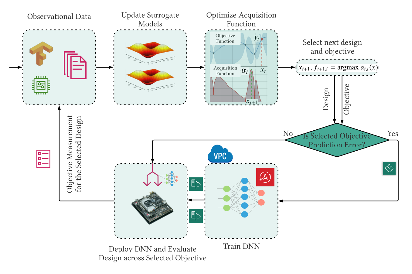
Figure 9 gives a high-level overview of our experimental setup. We implement FlexiBO in a distributed manner where the training of a DNN is done remotely on virtual machine instances with $8$ NVIDIA Tesla K80 GPU deployed on the Google cloud and the measurements and optimization algorithms run locally on resource-constrained Jetson devices, i.e. Xavier. Our experiments took a total of 5552.4 hours of wall-clock time to complete.

Hypervolume Error.

The Pareto hypervolume ( $\mathfrak{hv}$ ) is commonly used to measure the quality of an estimated Pareto front $\mathfrak{\hat{F}^{*}}$ (?, ?). As seen in Equation 11, it is defined as the volume enclosed by the estimated Pareto front $\mathfrak{\hat{F}^{*}}$ and a user-defined reference point $r$ in the objective space, in our case the origin of the coordinate system.

\mathfrak{hv}(\mathfrak{\hat{F}^{*}},r)=V(\cup_{s\in\mathfrak{\hat{F}^{*}}}\{q|r\preceq q\preceq s\})

(11)

The hypervolume error $\eta$ is defined as the difference between the hypervolumes of the true Pareto front $\mathfrak{F}^{*}$ and the estimated Pareto front $\hat{\mathfrak{F}}^{*}$ .

\eta=\mathfrak{hv}(\mathfrak{F^{*}},r)-\mathfrak{hv}(\mathfrak{\hat{F}^{*}},r)

(12)

Figure 10: Comparison of hypervolume error obtained by FlexiBO using different cost functions.

Figure 11: Comparison of Pareto optimal designs obtained by FlexiBO using different cost functions.

Figure 12: (a) Number of evaluations across each objective by FlexiBO using different cost functions (b) FlexiBO-GPLC achieved higher change of volume of the Pareto region with the recommended design and objective when compared to others.

We evaluate the quality of the obtained Pareto fronts using the hypervolume error and the cumulative log wall-clock time as the objective evaluation cost required to obtain it. As the actual Pareto fronts are unknown, we approximate them by combining the Pareto fronts obtained by the different optimization methods considered in our experiments.

6.2 Experimental Results

Given the same wall-clock time, we observe the hypervolume error obtained by Pareto fronts identified by the different optimization methods. Furthermore, to assess the quality of the Pareto fronts, we compare the number of designs in the target region of the objective space. Our target region is the region where the prediction error is less than 25% and energy consumption is less than the first quartile. Note that energy consumption is specific to the hardware platform.

Figure 13: Comparison of hypervolume error obtained by FlexiBO and other approaches for DNNs for object detection, NLP, and speech recognition applications.

Figure 14: Comparison of Pareto fronts obtained by FlexiBO and other approaches for DNNs for object detection, NLP, and speech recognition applications.

6.2.1 RQ1: Determination of objective evaluation cost function

Figures 10 and 11 show the results for optimizing prediction error and energy consumption with different cost functions. FlexiBO-GPLC has lower hypervolume error (shown in Figure 10) and a higher number of designs in the target region (shown in Figure 11) than FlexiBO-GPRC and FlexiBO-GPCC. To better understand the effect of different cost functions, we also look at the behavior of FlexiBO in Figure 12(a) and 12(b). Cost-unaware FlexiBO-GPCC greedily selects the design and objective across which the volume change is maximal for evaluation. As a result, FlexiBO-GPCC wastes resources by selecting expensive evaluations for little gain. This is evident from 12(b) which indicates that the reduction of volume by the designs selected by FlexiBO-GPCC are lower considering the evaluation cost. A larger change in the volume of Pareto region is desired as it indicates higher information gain. Objective evaluation cost function in FlexiBO-GPRC is skewed towards selecting the objective with lower evaluation cost and evaluates a higher number of designs for the less expensive objective e.g., energy consumption (shown in Figure 12(a)). However, it achieves lower change of the volume of the Pareto region than FlexiBO-GPLC. FlexiBO-GPLC on the other hand selects designs that achieved a larger volume change across the Pareto region (Figure 12(b)) and therefore a better choice than others.

6.2.2 RQ2: Effectiveness of FlexiBO

Effectiveness across DNNs of different applications.

Figures 13 and 14 show the effectiveness analysis of FlexiBO across different applications. In Figure 13 we observe that FlexiBO-GPLC outperforms other methods in finding Pareto fronts with lower hypervolume error for each of the applications. For example, FlexiBO achieves $22.4\%$ lower hypervolume error than CA-MOBO in DeepSpeech. In Figure 14, we observe that FlexiBO-GPLC is able to find a higher number of designs in the target region than other methods for ResNet, BERT-SQuAD, and DeepSpeech.

Figure 15: Comparison of hypervolume error obtained by FlexiBO and other approaches for DNNs of different sizes.

Figure 16: Comparison of Pareto fronts obtained by FlexiBO and other approaches for DNNs of different sizes.

Figure 17: FlexiBO utilizes resources more efficiently than other approaches when the difference of evaluation cost between objectives is high. The colors indicate the evaluation cost. FlexiBO is able to run for more iterations as it expends less of the evaluation budget at each one.

Effectiveness across DNNs of different sizes.

Figures 15 and 16 show the effectiveness analysis of FlexiBO across different-size DNNs. We make the following observations: (a) as shown in Figure 15, we find that FlexiBO-GPLC outperforms other methods in finding Pareto fronts with lower hypervolume error across all applications (e.g. $22.3\%$ lower for IMDB than CA-MOBO), (b) in Figure 16, we observe that FlexiBO-GPLC is able to find a higher number of designs in the target region than other methods for Xception, MobileNet, and BERT-IMDB. For LeNet, PAL achieves a $3.6\%$ lower hypervolume error than FlexiBO-GPLC. LeNet is a small architecture and FlexiBO performs poorly for such small architectures as the effect of selecting designs based on change of volume of the Pareto region per cost is less pronounced than for larger architectures (Xception or BERT-IMDB etc).

Table 6: Time (in seconds) required for one iteration with and without objective evaluation across all architectures.

	FlexiBO	PESMO	PESMO-DEC	PAL	CA-MOBO	ParEGO	SMSego
No Evaluation	79.9 $\pm$ 7.4	64.8 $\pm$ 5.1	66.9 $\pm$ 5.4	178.2 $\pm$ 10.6	71.2 $\pm$ 8.4	56.2	48.4 $\pm$ 4.3
With Evaluation	1417.2 $\pm$ 97.6	9133.7 $\pm$ 448.8	4400.4 $\pm$ 225.9	8764.3 $\pm$ 469.5	8411.5 $\pm$ 365.4	8656.9 $\pm$ 220.3	9020.9 $\pm$ 306.3

We observe that approaches other than FlexiBO cannot make the best use of the allocated budget as they evaluate the more expensive objectives more than the cheap objectives. As the expensive objectives can be selected any time (even for little gain), this strategy is wasteful when limited resources are available. FlexiBO makes better use of the resources by evaluating the cheaper objectives more in the earlier iterations and thus gaining a better understanding of the design space and only later evaluating the costly objective (Figure 17). We also find that FlexiBO is able to evaluate more designs by prudently selecting the objectives across which to evaluate it (Figures 15 and 16). A cost-aware decoupled approach is clearly useful for scenarios where the evaluation budget is limited.

Comparison of average time required for modeling.

Table 6 shows the average time required for one iteration for different multi-objective optimization methods, averaged across all architectures. Though FlexiBO requires more time to compute the acquisition function (no evaluation) than others, the time required for one iteration including the objective evaluation time in FlexiBO is $5.6\times$ lower than the next best method ParEGO.

6.2.3 RQ3: Sensitivity Analysis

Figure 18: Comparison of hypervolume error obtained by FlexiBO with different surrogate models.

Figure 19: Comparison of Pareto fronts obtained by FlexiBO with different surrogate models.

Different surrogate models.

We compare the performance of the different variants of FlexiBO: FlexiBO-GPLC and FlexiBO-RFLC that use log objective evaluation cost. We used this cost function as it is a better choice than ratio and constant cost functions. Figures 18 and 19 show the hypervolume error and quality of the obtained Pareto fronts. We find that across all architectures FlexiBO-GPLC outperforms FlexiBO-RFLC (FlexiBO-GPLC has lower hypervolume error and higher number of designs in the target region).

7 Conclusion

In this work, we proposed a novel cost-aware acquisition function for Bayesian multi-objective optimization called FlexiBO. Instead of evaluating all objective functions, FlexiBO automatically chooses the one that provides the highest benefit, weighted by the cost to perform the evaluation. We showed the promise of our approach through an extensive and thorough evaluation of seven different DNN architectures over a large design space on resource-constrained hardware platforms. Our experimental results show that FlexiBO performs better than current state-of-the-art approaches in most cases, both in terms of the quality of the obtained Pareto fronts and the cost necessary to obtain them.

Acknowledgements

This work has been supported, in part, by NSF (Awards 2007202 and 2107463), as well as Google and Chameleon Cloud (provided cloud resources for the experiments). We are grateful to all who provided feedback on the earlier versions of this work, including Luigi Nardi (and several members of his group at Lund), Mohammad Ali Javidian, Md Abir Hossen, several members of ABLE Research Group at CMU, and anonymous reviewers of AutoML’22.

References

Abdolshah et al. Abdolshah, M., Shilton, A., Rana, S., Gupta, S., & Venkatesh, S. (2019a). Cost-aware multi-objective bayesian optimisation..
Abdolshah et al. Abdolshah, M., Shilton, A., Rana, S., Gupta, S., & Venkatesh, S. (2019b). Multi-objective bayesian optimisation with preferences over objectives..
Acher et al. Acher, M., Martin, H., Pereira, J., Blouin, A., Jézéquel, J.-M., Khelladi, D., Lesoil, L., & Barais, O. (2019). Learning very large configuration spaces: What matters for linux kernel sizes..
Belakaria et al. Belakaria, S., Deshwal, A., & Doppa, J. R. (2019). Max-value entropy search for multi-objective bayesian optimization. In Advances in Neural Information Processing Systems, pp. 7825–7835.
Belakaria et al. Belakaria, S., Deshwal, A., & Doppa, J. R. (2020). Max-value entropy search for multi-objective bayesian optimization with constraints..
Cai et al. Cai, E., Juan, D.-C., Stamoulis, D., & Marculescu, D. (2017). Neuralpower: Predict and deploy energy-efficient convolutional neural networks..
Cai et al. Cai, H., Zhu, L., & Han, S. (2018). Proxylessnas: Direct neural architecture search on target task and hardware..
Campigotto et al. Campigotto, P., Passerini, A., & Battiti, R. (2013). Active learning of pareto fronts. IEEE transactions on neural networks and learning systems, 25(3), 506–519.
Cao et al. Cao, Y., Smucker, B. J., & Robinson, T. J. (2015). On using the hypervolume indicator to compare pareto fronts: Applications to multi-criteria optimal experimental design. Journal of Statistical Planning and Inference, 160, 60–74.
Chen et al. Chen, Y.-H., Emer, J., & Sze, V. (2016). Eyeriss: A spatial architecture for energy-efficient dataflow for convolutional neural networks. In ACM SIGARCH Computer Architecture News, Vol. 44, pp. 367–379. IEEE Press.
Chen et al. Chen, Y.-H., Yang, T.-J., Emer, J., & Sze, V. Understanding the limitations of existing energy-efficient design approaches for deep neural networks. Energy, 2(L1), L3.
Chollet Chollet, F. (2017). Xception: Deep learning with depthwise separable convolutions. In Proceedings of the IEEE conference on computer vision and pattern recognition, pp. 1251–1258.
Deb Deb, K. (2001). Multi-objective optimization using evolutionary algorithms, Vol. 16. John Wiley & Sons.
Deb & Sundar Deb, K., & Sundar, J. (2006). Reference point based multi-objective optimization using evolutionary algorithms. In Proceedings of the 8th annual conference on Genetic and evolutionary computation, pp. 635–642. ACM.
Désidéri Désidéri, J.-A. (2012). Multiple-gradient descent algorithm (mgda) for multiobjective optimization. Comptes Rendus Mathematique, 350(5-6), 313–318.
Devlin et al. Devlin, J., Chang, M.-W., Lee, K., & Toutanova, K. (2018). Bert: Pre-training of deep bidirectional transformers for language understanding..
Dong et al. Dong, J.-D., Cheng, A.-C., Juan, D.-C., Wei, W., & Sun, M. (2018). Dpp-net: Device-aware progressive search for pareto-optimal neural architectures. In Proceedings of the European Conference on Computer Vision (ECCV), pp. 517–531.
Emmerich & Klinkenberg Emmerich, M., & Klinkenberg, J.-w. (2008). The computation of the expected improvement in dominated hypervolume of pareto front approximations. Rapport technique, Leiden University, 34, 7–3.
Gadepally et al. Gadepally, V., Goodwin, J., Kepner, J., Reuther, A., Reynolds, H., Samsi, S., Su, J., & Martinez, D. (2019). Ai enabling technologies: A survey..
Guo Guo, T. (2017). Towards efficient deep inference for mobile applications..
Halawa et al. Halawa, H., Abdelhafez, H. A., Boktor, A., & Ripeanu, M. (2017). Nvidia jetson platform characterization. In European Conference on Parallel Processing, pp. 92–105. Springer.
Hannun et al. Hannun, A., Case, C., Casper, J., Catanzaro, B., Diamos, G., Elsen, E., Prenger, R., Satheesh, S., Sengupta, S., Coates, A., et al. (2014). Deep speech: Scaling up end-to-end speech recognition..
He et al. He, K., Zhang, X., Ren, S., & Sun, J. (2016). Deep residual learning for image recognition. In Proceedings of the IEEE conference on computer vision and pattern recognition, pp. 770–778.
Hernández-Lobato et al. Hernández-Lobato, D., Hernandez-Lobato, J., Shah, A., & Adams, R. (2016). Predictive entropy search for multi-objective bayesian optimization. In International Conference on Machine Learning, pp. 1492–1501.
Hernández-Lobato et al. Hernández-Lobato, J. M., Gelbart, M. A., Hoffman, M. W., Adams, R. P., & Ghahramani, Z. (2015). Predictive entropy search for bayesian optimization with unknown constraints.. JMLR.
Hernández-Lobato et al. Hernández-Lobato, J. M., Gelbart, M. A., Reagen, B., Adolf, R., Hernández-Lobato, D., Whatmough, P. N., Brooks, D., Wei, G.-Y., & Adams, R. P. (2016). Designing neural network hardware accelerators with decoupled objective evaluations. In NIPS workshop on Bayesian Optimization, p. 10.
Hernández-Lobato et al. Hernández-Lobato, J. M., Hoffman, M. W., & Ghahramani, Z. (2014). Predictive entropy search for efficient global optimization of black-box functions. In Advances in neural information processing systems, pp. 918–926.
Iandola et al. Iandola, F. N., Han, S., Moskewicz, M. W., Ashraf, K., Dally, W. J., & Keutzer, K. (2016). Squeezenet: Alexnet-level accuracy with 50x fewer parameters and< 0.5 mb model size..
Iqbal et al. Iqbal, M. S., Kotthoff, L., & Jamshidi, P. (2019). Transfer Learning for Performance Modeling of Deep Neural Network Systems. In USENIX Conference on Operational Machine Learning, Santa Clara, CA. USENIX Association.
Jamshidi & Casale Jamshidi, P., & Casale, G. (2016). An uncertainty-aware approach to optimal configuration of stream processing systems. In Proc. Int’l Symp. on Modeling, Analysis and Simulation of Computer and Telecommunication Systems (MASCOTS). IEEE.
Jamshidi et al. Jamshidi, P., Velez, M., Kästner, C., & Siegmund, N. (2018). Learning to sample: Exploiting similarities across environments to learn performance models for configurable systems. In Proc. Int’l Symp. Foundations of Software Engineering (FSE). ACM.
Jamshidi et al. Jamshidi, P., Velez, M., Kästner, C., Siegmund, N., & Kawthekar, P. (2017). Transfer learning for improving model predictions in highly configurable software. In Proc. Int’l Symp. Soft. Engineering for Adaptive and Self-Managing Systems (SEAMS). IEEE.
Jones et al. Jones, D. R., Schonlau, M., & Welch, W. J. (1998). Efficient Global Optimization of Expensive Black-Box Functions. J. of Global Optimization, 13(4), 455–492.
Kim et al. Kim, J.-H., Han, J.-H., Kim, Y.-H., Choi, S.-H., & Kim, E.-S. (2011). Preference-based solution selection algorithm for evolutionary multiobjective optimization. IEEE Transactions on Evolutionary Computation, 16(1), 20–34.
Kim et al. Kim, Y.-H., Reddy, B., Yun, S., & Seo, C. (2017). Nemo: Neuro-evolution with multiobjective optimization of deep neural network for speed and accuracy. In ICML 2017 AutoML Workshop.
Knowles Knowles, J. (2006). Parego: a hybrid algorithm with on-line landscape approximation for expensive multiobjective optimization problems. IEEE Transactions on Evolutionary Computation, 10(1), 50–66.
Kolesnikov et al. Kolesnikov, S., Siegmund, N., Kästner, C., Grebhahn, A., & Apel, S. (2019). Tradeoffs in modeling performance of highly configurable software systems. Software & Systems Modeling, 18(3), 2265–2283.
Krizhevsky et al. Krizhevsky, A., Hinton, G., et al. (2009). Learning multiple layers of features from tiny images.. Citeseer.
Kung et al. Kung, H.-T., Luccio, F., & Preparata, F. P. (1975). On finding the maxima of a set of vectors. Journal of the ACM (JACM), 22(4), 469–476.
LeCun & Cortes LeCun, Y., & Cortes, C. (2010). MNIST handwritten digit database..
LeCun et al. LeCun, Y., et al. (2015). Lenet-5, convolutional neural networks. URL: http://yann. lecun. com/exdb/lenet, 20(5), 14.
Lee et al. Lee, E. H., Perrone, V., Archambeau, C., & Seeger, M. (2020). Cost-aware bayesian optimization..
Liu et al. Liu, H., Simonyan, K., Vinyals, O., Fernando, C., & Kavukcuoglu, K. (2017). Hierarchical representations for efficient architecture search..
Lokhmotov et al. Lokhmotov, A., Chunosov, N., Vella, F., & Fursin, G. (2018). Multi-objective autotuning of mobilenets across the full software/hardware stack. In Proceedings of the 1st on Reproducible Quality-Efficient Systems Tournament on Co-designing Pareto-efficient Deep Learning, p. 6. ACM.
Manotas et al. Manotas, I., Pollock, L., & Clause, J. (2014). Seeds: a software engineer’s energy-optimization decision support framework. In Proceedings of the 36th International Conference on Software Engineering, pp. 503–514. ACM.
Mozilla Mozilla (2019). https://commonvoice.mozilla.org/en/datasets.
Nair et al. Nair, V., Yu, Z., Menzies, T., Siegmund, N., & Apel, S. (2018). Finding faster configurations using flash.. IEEE.
Nardi et al. Nardi, L., Koeplinger, D., & Olukotun, K. (2019). Practical design space exploration. In 2019 IEEE 27th International Symposium on Modeling, Analysis, and Simulation of Computer and Telecommunication Systems (MASCOTS), pp. 347–358. IEEE.
Paria et al. Paria, B., Kandasamy, K., & Póczos, B. (2018). A flexible framework for multi-objective bayesian optimization using random scalarizations..
Pei et al. Pei, K., Cao, Y., Yang, J., & Jana, S. (2017). Deepxplore: Automated whitebox testing of deep learning systems. In proceedings of the 26th Symposium on Operating Systems Principles, pp. 1–18.
Peitz & Dellnitz Peitz, S., & Dellnitz, M. (2018). Gradient-based multiobjective optimization with uncertainties. In NEO 2016, pp. 159–182. Springer.
Pereira et al. Pereira, J. A., Martin, H., Acher, M., Jézéquel, J.-M., Botterweck, G., & Ventresque, A. (2019). Learning software configuration spaces: A systematic literature review..
Picheny Picheny, V. (2015). Multiobjective optimization using gaussian process emulators via stepwise uncertainty reduction. Statistics and Computing, 25(6).
Poirion et al. Poirion, F., Mercier, Q., & Désidéri, J.-A. (2017). Descent algorithm for nonsmooth stochastic multiobjective optimization. Computational Optimization and Applications, 68(2), 317–331.
Ponweiser et al. Ponweiser, W., Wagner, T., Biermann, D., & Vincze, M. (2008). Multiobjective optimization on a limited budget of evaluations using model-assisted $\{$ S $\}$ -metric selection. In International Conference on Parallel Problem Solving from Nature, pp. 784–794. Springer.
Qi et al. Qi, H., Sparks, E. R., & Talwalkar, A. (2016). Paleo: A performance model for deep neural networks..
Rajpurkar et al. Rajpurkar, P., Zhang, J., Lopyrev, K., & Liang, P. (2016). Squad: 100,000+ questions for machine comprehension of text..
Rasmussen Rasmussen, C. E. (2003). Gaussian processes in machine learning. In Summer School on Machine Learning, pp. 63–71. Springer.
Reuther et al. Reuther, A., Michaleas, P., Jones, M., Gadepally, V., Samsi, S., & Kepner, J. (2019). Survey and benchmarking of machine learning accelerators. In 2019 IEEE high performance extreme computing conference (HPEC), pp. 1–9. IEEE.
Roijers et al. Roijers, D. M., Vamplew, P., Whiteson, S., & Dazeley, R. (2013). A survey of multi-objective sequential decision-making. Journal of Artificial Intelligence Research, 48, 67–113.
Roijers et al. Roijers, D. M., Zintgraf, L. M., Libin, P., & Nowé, A. (2018). Interactive multi-objective reinforcement learning in multi-armed bandits for any utility function. In ALA workshop at FAIM, Vol. 8.
Roijers et al. Roijers, D. M., Zintgraf, L. M., & Nowé, A. (2017). Interactive thompson sampling for multi-objective multi-armed bandits. In International Conference on Algorithmic DecisionTheory. Springer.
Rouhani et al. Rouhani, B. D., Mirhoseini, A., & Koushanfar, F. (2016). Delight: Adding energy dimension to deep neural networks. In Proceedings of the 2016 International Symposium on Low Power Electronics and Design, pp. 112–117. ACM.
Russakovsky et al. Russakovsky, O., Deng, J., Su, H., Krause, J., Satheesh, S., Ma, S., Huang, Z., Karpathy, A., Khosla, A., Bernstein, M., et al. (2015). Imagenet large scale visual recognition challenge. International journal of computer vision, 115(3), 211–252.
Sandler et al. Sandler, M., Howard, A., Zhu, M., Zhmoginov, A., & Chen, L.-C. (2018). Mobilenetv2: Inverted residuals and linear bottlenecks. In Proceedings of the IEEE conference on computer vision and pattern recognition, pp. 4510–4520.
Schäffler et al. Schäffler, S., Schultz, R., & Weinzierl, K. (2002). Stochastic method for the solution of unconstrained vector optimization problems. Journal of Optimization Theory and Applications, 114(1), 209–222.
Shapiro Shapiro, A. (2003). Monte carlo sampling methods. Handbooks in operations research and management science, 10, 353–425.
Srinivas et al. Srinivas, N., Krause, A., Kakade, S. M., & Seeger, M. W. (2012). Information-theoretic regret bounds for gaussian process optimization in the bandit setting. IEEE Transactions on Information Theory, 58(5), 3250–3265.
Sun et al. Sun, Y., Wu, M., Ruan, W., Huang, X., Kwiatkowska, M., & Kroening, D. (2018). Concolic testing for deep neural networks. In Proceedings of the 33rd ACM/IEEE International Conference on Automated Software Engineering, pp. 109–119.
Sze et al. Sze, V., Chen, Y.-H., Yang, T.-J., & Emer, J. S. (2017). Efficient processing of deep neural networks: A tutorial and survey. Proceedings of the IEEE, 105(12), 2295–2329.
Thiele et al. Thiele, L., Miettinen, K., Korhonen, P. J., & Molina, J. (2009). A preference-based evolutionary algorithm for multi-objective optimization. Evolutionary computation, 17(3), 411–436.
Wang & Jegelka Wang, Z., & Jegelka, S. (2017). Max-value entropy search for efficient bayesian optimization..
Whatmough et al. Whatmough, P. N., Zhou, C., Hansen, P., Venkataramanaiah, S. K., Seo, J.-s., & Mattina, M. (2019). Fixynn: Efficient hardware for mobile computer vision via transfer learning..
Wu et al. Wu, B., Dai, X., Zhang, P., Wang, Y., Sun, F., Wu, Y., Tian, Y., Vajda, P., Jia, Y., & Keutzer, K. (2019). Fbnet: Hardware-aware efficient convnet design via differentiable neural architecture search. In Proceedings of the IEEE Conference on Computer Vision and Pattern Recognition, pp. 10734–10742.
Zela et al. Zela, A., Klein, A., Falkner, S., & Hutter, F. (2018). Towards automated deep learning: Efficient joint neural architecture and hyperparameter search..
Zhu et al. Zhu, Y., Mattina, M., & Whatmough, P. (2018). Mobile machine learning hardware at arm: A systems-on-chip (soc) perspective..
Zintgraf et al. Zintgraf, L. M., Roijers, D. M., Linders, S., Jonker, C. M., & Nowé, A. (2018). Ordered preference elicitation strategies for supporting multi-objective decision making. In Proceedings of the 17th International Conference on Autonomous Agents and MultiAgent Systems, pp. 1477–1485. International Foundation for Autonomous Agents and Multiagent Systems.
Zitzler & Thiele Zitzler, E., & Thiele, L. (1999). Multiobjective evolutionary algorithms: a comparative case study and the strength pareto approach. IEEE Transactions on Evolutionary Computation, 3(4), 257–271.
Zuluaga et al. Zuluaga, M., Krause, A., & Püschel, M. (2016). $\varepsilon$ -pal: an active learning approach to the multi-objective optimization problem. The Journal of Machine Learning Research, 17(1), 3619–3650.
Zuluaga et al. Zuluaga, M., Sergent, G., Krause, A., & Püschel, M. (2013). Active learning for multi-objective optimization. In International Conference on Machine Learning, pp. 462–470.

8 Appendix

In this section, we analyze the sample complexity of FlexiBO.

Table 7: List of symbols and their descriptions.

Symbol	Description

$t$	Number of iteration
$P_{R}$	Pareto region
$T$	Total number of iterations
$\mathfrak{F}_{pess}$	Pessimistic Pareto front
$n$	Number of objectives
$V_{t}$	Volume of $P_{R}$ at iteration $t$
$\mu$	Posterior mean
$\sigma$	Posterior standard deviation
$\mathfrak{U}$	Non-dominated points set
$\theta_{t,i}$	Evaluation cost of an objective $f_{i}$
$\bm{x}$	A design
$r$	A reference point
$\mathfrak{X}$	Design space
$\Delta V_{t}$	Change of volume of the $P_{R}$ at iteration $t$
$f$	An objective
$R_{t}(\bm{x})$	Uncertainty region of a point $\bm{x}$ at iteration $t$
$\beta_{t}$	Scaling parameter value at iteration $t$
$\mathfrak{M}$	Surrogate model
$S_{i}$	Evaluated points set for objective $f_{i}$
$\mathfrak{F}^{*}$	Optimal Pareto front
$\mathfrak{X}^{*}$	Pareto-optimal set
$N_{0}$	Number of initial samples
$\eta$	Pareto hypervolume error
$\mathfrak{hv}$	Pareto hypervolume
$\theta_{T}$	Total objective evaluation cost
$\delta$	Probability
$\gamma_{T}$	Maximum information gain
$\alpha$	Acquisition function
$\Delta^{n}$	n-simplex
$V(\Delta^{n})$	Volume of an n-simplex
$k$	Co-variance
$y_{i}$	Actual value of an objective $f_{i}$
$v$	Measurement noise
$\hat{\mathfrak{F}^{*}}$	Approximate optimal Pareto front

Let us assume that the maximum iteration within budget $\theta_{T}$ is $T$ . By extending the theory from PAL, we derive the convergence rate of our proposed FlexiBO algorithm. (?) demonstrated that the critical quantity governing the convergence rate is given by the following:

\gamma_{T}=\max_{\bm{y}_{1}...\bm{y}_{T}}I(\bm{y}_{1}...\bm{y}_{T};\bm{f}),

(13)

i.e., maximum reduction of uncertainty achievable by sampling $T$ designs. For FlexiBO, the maximum reduction of uncertainty corresponds to the maximum change of the volume of the Pareto region $\Delta V$ and the above equation can be written as:

\gamma_{T}=\max_{\bm{y}_{1}...\bm{y}_{T}}\Delta V(\bm{y}_{1}...\bm{y}_{T};\bm{f}),

(14)

Similar to (?, ?), we also establish $\gamma_{T}$ as the key quantity in bounding the hypervolume error $\eta$ in our analysis. The following theorem is our main theoretical result.

Figure 20: Example of hypervolume error bound for two objectives.

Theorem 1.

Let $\delta\in(0,1)$ . FlexiBO running with $\beta_{t}=2/9\log(n|\mathfrak{X}|\pi^{2}t^{2}/{6\delta})$ would achieve a maximum hypervolume error of $\eta$ of the Pareto front obtained inside total cost $\theta_{T}$ with probability $1-\delta$ .

\eta\leq\frac{\sqrt{n}a^{n-1}}{(n-1)!}\left\{a^{n}-2\Big(\frac{C_{1}\beta_{T}\gamma_{T}}{2}\Big)^{n/2}{\frac{(\frac{\theta_{T}}{\theta_{x}}(n+1))^{1/2}}{n!}}\right\}

(15)

Here, $a_{i}=\max_{\bm{x}\in\mathfrak{X_{m}},1\leq i\leq n}{\sigma_{i}(\bm{x})\sqrt{\beta_{1}}}$ , $C_{1}=\frac{8}{\log(1+\sigma^{-2)}}$ , $\theta_{x}=\frac{\sum_{i=1}^{n}\theta_{i}}{n}$ and $\gamma_{T}$ It depends on the type of surrogate because the predicted uncertainty can differ depending on a model’s ability to handle noisy measurements.

This indicates that by specifying $\delta$ and a total budget $\theta_{T}$ , FlexiBO can be configured to achieve a hypervolume error $\eta$ with confidence $1-\delta$ .

Proof.

Initially, using Lemma 1 and 2, we show how the change of volume of the Pareto region $\sum_{t=1}^{T}\Delta V_{t,i}$ is related to the total budget $\theta_{T}$ :

\displaystyle\sum_{t=1}^{T}\Delta{V}_{t,i}\leq 2\Big(\frac{C_{1}\beta_{T}\gamma_{T}}{2}\Big)^{n/2}{\frac{(\frac{\theta_{T}}{\theta_{x}}(n+1))^{1/2}}{n!}}

Now, we relate hypervolume error $\eta$ and $\theta_{T}$ . Let $1_{n}=(1,...,1)^{T}$ and let $e_{i}$ denote the $i^{th}$ canonical base vector. (?) that considers $a_{i}$ to be the maximum value for each $f_{i}(x)$ , with probability $1-\delta$ . Here, $a_{i}=\max_{\bm{x}\in\mathfrak{X_{m}},1\leq i\leq n}{\sigma_{i}(\bm{x})\sqrt{\beta_{1}}}$ obtained from the width of the confidence regions, as shown in Figure 20. We obtain this by replacing the co-variance term $k_{i}(\bm{x},\bm{x})$ used for measuring the width of the confidence region only for GP in Lemma 12 by (?) with variance $\sigma_{i}^{2}(\bm{x})$ to extend our proof for both GP and RF surrogate models. PAL (?) also showed that the projection $a_{i}$ , where $1\leq i\leq n$ , onto the hyperplane $H_{n}$ is an n-simplex $S_{n}$ has a volume of $\frac{\sqrt{n}a^{n-1}}{(n-1)!}$ . Hypervolume error $\eta$ depends on the distance between the boundaries defined by $\mathfrak{F}_{pess}$ and $\mathfrak{F}_{opt}$ at any iteration that is bounded by $\frac{\sqrt{n}a^{n-1}}{(n-1)!}{V}_{t}$ (?). At any iteration $t$ , $V_{t}$ can be written as the difference between initial volume of the Pareto region $V_{1}$ and sum of change of volume $\Delta V_{t}$ . At iteration $T$ , hypervolume error $\eta$ can be written as the following:

	$\displaystyle\eta$	$\displaystyle\leq\frac{\sqrt{n}a^{n-1}}{(n-1)!}\left\{V_{1}-\sum_{t=1}^{T}\Delta V_{t,i}\right\}$
		$\displaystyle\leq\frac{\sqrt{n}a^{n-1}}{(n-1)!}\left\{a^{n}-2\Big(\frac{C_{1}\beta_{T}\gamma_{T}}{2}\Big)^{n/2}{\frac{(\frac{\theta_{T}}{\theta_{x}}(n+1))^{1/2}}{n!}}\right\}\ \text{where}\ V_{1}=a^{n}$

∎

Figure 21: Example Pareto region

P_{R}

for

n=2

objectives (left). The Pareto region is a sum of n-simplexes (middle). The change of volume after evaluation across objective

f_{1}

is shown by the yellow region (right).

Lemma 1.

Given $\delta\in(0,1)$ and $\beta_{t}=2/9\log(n|\mathfrak{X_{m}}|\pi^{2}t^{2}/{6\delta})$ , the following holds with probability $\leq 1-\delta$ with $C_{1}=\frac{8}{\log(1+\sigma^{-2})}$ .

\sum_{t=1}^{T}\Delta{V}_{t,i}{{}^{2}}\leq\frac{4(C_{1}\beta_{T}\gamma_{T})^{n}}{(n!)^{2}}\frac{n+1}{2^{n}},

(16)

Proof.

The change of volume of the Pareto region at any iteration $t$ would be across only one objective $f_{i}$ , where $1\leq i\leq n$ . Therefore, we need to determine the change of volume $\Delta V_{t,i}$ for $f_{i}$ only. Let us assume that $m$ is the centroid of the Pareto region $P_{R}$ . If we add each vertex of the uncertainty region $R_{t}(\bm{x})$ of each design $\bm{x}$ with centroid $m$ an n-simplex is formed. So, the Pareto region $P_{R}$ can be shown as the sum of all these n-simplexes similar to Figure 21 (middle). When a design $\bm{x}_{t}$ is evaluated across an objective, volume of the Pareto region is reduced by the volume of two n-simplexes as shown by the yellow region in Figure 21 (right) i.e., an n-simplex becomes n-1-simplex due to reduction of uncertainty. Volume of an n-simplex is given by $\frac{s^{n}}{n!}\sqrt{\frac{n+1}{2^{n}}}$ , where $s$ is the length of the side.

	$\displaystyle\Delta{V}_{t,i}$	$\displaystyle\leq 2V(\Delta^{n})$
		$\displaystyle\leq\frac{2s^{n}}{n!}\sqrt{\frac{n+1}{2^{n}}}$

By using the width of the uncertainty region $2\beta_{t}^{1/2}\sigma_{t-1,i}(\bm{x}_{t})$ across an objective $f_{i}$ as the side length $s$ we get the following:

\displaystyle\Delta{V}_{t,i}

\displaystyle\leq\frac{2(2\beta_{t}^{1/2}\sigma_{t-1,i}(\bm{x}_{t}))^{n}}{n!}\sqrt{\frac{n+1}{2^{n}}}

where $1\leq i\leq n$ . As $\beta_{t}$ is increasing the above equation can be written similar to (?) by the following:

	$\displaystyle\Delta{V}_{t,i}^{2}$	$\displaystyle\leq\frac{4(4\beta_{T}\sigma^{2}(\sigma^{-2}\sigma_{t-1,i}^{2}(\bm{x}_{t})))^{n}}{(n!)^{2}}\frac{n+1}{2^{n}}$
		$\displaystyle\leq\frac{4(4\beta_{T}\sigma^{2}C_{2}\log(1+\sigma^{-2}\sigma_{t-1,i}^{2}(\bm{x}_{t})))^{n}}{(n!)^{2}}\frac{n+1}{2^{n}},$

where $C_{2}=\frac{\sigma^{-2}}{\log(1+\sigma^{-2})}$ . Applying summation on the above we get

\displaystyle\sum_{t=1}^{T}\Delta{V}_{t,i}^{2}\leq\frac{4(4\beta_{T}\sigma^{2}C_{2}\sum_{t=1}^{T}\log(1+\sigma^{-2}\sigma_{t-1,i}^{2}(\bm{x}_{t})))^{n}}{(n!)^{2}}\frac{n+1}{2^{n}}

With $C_{1}=8\sigma^{2}C_{2}$ we get the following:

	$\displaystyle\sum_{t=1}^{T}\Delta V_{t,i}^{2}$	$\displaystyle\leq\frac{4(4\beta_{T}\sigma^{2}C_{2}\Delta V(\bm{y}_{T};\bm{f}_{T},i))^{n}}{(n!)^{2}}\frac{n+1}{2^{n}}$
		$\displaystyle\leq\frac{4(C_{1}\beta_{T}\Delta V(\bm{y}_{T};\bm{f}_{T}))^{n}}{(n!)^{2}}\frac{n+1}{2^{n}}$
		$\displaystyle\leq\frac{4(C_{1}\beta_{T}\gamma_{T})^{n}}{(n!)^{2}}\frac{n+1}{2^{n}}$

∎

Lemma 2.

Given $\delta\in(0,1)$ and $\beta_{t}=2/9\log(n|\mathfrak{X_{m}}|\pi^{2}t^{2}/{6\delta})$ , the following holds with probability $\leq 1-\delta$ .

\sum_{t=1}^{T}\Delta{V}_{t,i}\leq 2\Big(\frac{C_{1}\beta_{T}\gamma_{T}}{2}\Big)^{n/2}{\frac{(\frac{\theta_{T}}{\theta_{x}}(n+1))^{1/2}}{n!}}\ for\ T\geq 1

(17)

Proof.

Similar to Lemma 6 in (?), by applying Cauchy-Schwarz inequality on Lemma 1 as $(\sum_{t=1}^{T}\Delta{V}_{t,i})^{2}\leq T\sum_{t=1}^{T}\Delta{V}_{t,i}^{2}$ , we obtain the following:

\sum_{t=1}^{T}\Delta{V}_{t,i}\leq 2\Big(\frac{C_{1}\beta_{T}\gamma_{T}}{2}\Big)^{n/2}{\frac{(T(n+1))^{1/2}}{n!}}\ for\ T\geq 1

(18)

In the worst case, $T\leq\frac{\theta_{T}}{\theta_{x}}$ , where $\theta_{x}=\frac{\sum_{i=1}^{n}\theta_{i}}{n}$ .

∎

8.1 Runtime Complexity of FlexiBO

We analyze the run-time complexity of FlexiBO using Gaussian Processes (GP) and random forests (RF) as surrogate models, separately, in this section. The total complexity of FlexiBO can be determined by combining complexities of FlexiBO from modeling, Pareto region construction, and sampling stages.

Let $|\mathfrak{X}|=q$ be the total number of designs in the design space. However, we only consider $|\mathfrak{X}_{m}|=m$ designs sampled by Monte-Carlo sampling in this approach. We also consider $N_{0}+t$ designs to train the surrogate models at each iteration $t$ . Let us consider $s=m+N_{0}+t$ . Note that by design, $s<<q$ . As a result, our FlexiBO algorithm is significantly faster.

Modeling.

In the modeling stage, only a small subset of designs are used to train the surrogate models at each iteration. Training a GP with $s$ number of designs takes $\mathcal{O}(s^{3}+ms^{2})$ (?) time. Training a RF with $s$ designs takes $\mathcal{O}(n_{t}n_{v}s^{2}\log s)$ time where $n_{t}$ is the number of trees, and $n_{v}$ is the number of features used at each level. Determining the uncertainty region of each design $\bm{x}\in\mathfrak{X_{m}}$ takes an additional $\mathcal{O}(m)$ time. Therefore, total complexity of the modeling stage for using GP surrogate model is $\mathcal{O}(s^{3}+ms^{2}+m)$ and for RF surrogate model is $\mathcal{O}(n_{t}n_{v}s^{2}\log s+m)$ .

Pareto Region Construction.

In the Pareto region construction stage, we initially determine the non-dominated designs in the design space and later use the non-dominated designs $\bm{x}\in\mathfrak{U}$ to construct the Pareto fronts. The complexity of finding the non-dominated designs is $\mathcal{O}(m^{2})$ . The complexity of constructing the Pareto fronts is similar to the complexity of determining the number of designs on the boundary of the convex hull, which can be performed in $\mathcal{O}(m\log m)|$ time if the number of objectives $n=2$ . When $n>2$ , the Pareto fronts are constructed in $\mathcal{O}(m(\log m)^{n-2}+m\log m)$ time (?).

Sampling.

In the sampling stage, FlexiBO determines the next sample $\bm{x}_{t}$ and objective $f_{t,i}$ for evaluation. To do so, FlexiBO computes the acquisition function $\alpha_{t,i}(\bm{x})$ for each design in $\mathfrak{X_{m}}^{*}$ and selects the maximum. To compute $\alpha_{t,i}(\bm{x})$ across an objective $f_{i}$ , FlexiBO needs to compute the volume of the Pareto region $P_{R}$ by updating the uncertainty values of $\bm{x}$ in $\mathfrak{X_{m}}^{*}$ . This would take $\mathcal{O}(m)$ time as $|\mathfrak{X_{m}}|^{*}=m$ in the worst case. After measuring the selected design $\bm{x}_{t}$ across objective $f_{t,i}$ , we update the evaluated designs set $S_{i}$ and objective evaluation cost $\theta_{t,i}$ . All of these are done in constant time and we can safely ignore them in our analysis. Therefore, the total run-time complexity of FlexiBO in the sampling stage is $O(m)$ , regardless of the surrogate model.

Overall.

Finally, we determine the overall complexity of FlexiBO using GP and RF for $n$ objectives by combining the complexities of the three stages discussed above. When GP is used as the surrogate model, the total complexity of FlexiBO for $n=2$ objectives is $\mathcal{O}(s^{3}+ms^{2}+m^{2}+m\log m+2m)$ and for $n\geq 3$ objectives the total complexity is $\mathcal{O}(s^{3}+ms^{2}+m^{2}+m(\log m)^{n-2}+m\log m+2m)$ . To simplify these expressions, we consider $s=m$ . Now, the total complexity for $n=2$ objectives using GP surrogate model is approximately $\mathcal{O}(s^{3}+s^{2}+s\log s+s)$ and for $n=3$ objectives is $\mathcal{O}(s^{3}+s^{2}+s(\log s)^{n-2}+s\log s+s)$ .

Similarly when RF is used as a surrogate model, the total complexity of FlexiBO for $n=2$ objectives is $\mathcal{O}(n_{t}n_{v}s^{2}\log s+m^{2}+m\log m+2m)$ and for $n\geq 3$ objectives is $\mathcal{O}(n_{t}n_{v}s^{2}\log s+m^{2}+m(\log m)^{n-2}+m\log m+2m)$ . After simplification the complexity for $n=2$ objectives can be written as $\mathcal{O}(s^{2}\log s+s^{2}+s\log s+s)$ and for $n=3$ objectives the complexity can be rewritten as $\mathcal{O}(s^{2}\log s+s^{2}+s(\log s)^{n-2}+s\log s+s)$ .

Upon further simplification, we observe that the complexity of FlexiBO with the GP surrogate model is approximately $\mathcal{O}(s^{3})$ and for the RF surrogate model the complexity is $\mathcal{O}(s^{2}\log s)$ , where $s$ is significantly lower than the total number of designs $q$ .