Persistent spin textures and currents in wurtzite nanowire-based quantum structures

The bulk electrons in the $\Gamma_{\text{7c}}$ conduction band of a wurtzite type semiconductor with SOC are described by the Hamiltonian

The kinetic part of the Hamiltonian is axially symmetric and reads

where $k_{\perp}^{2}=k_{x}^{2}+k_{y}^{2}$, $m_{z}$ denotes the effective electron mass along the $z$-axis and $m_{\perp}$ the according perpendicular component. In this notation, the $z$-axis corresponds to the [0001] wurtzite crystal axis (c-axis) and, at the same time, the nanowire axis. The SOC yields the intrinsic (int) and extrinsic (ext) contributionsFu and Wu 2008; Faria Junior et al. 2016; Zutic et al. 2004; Gmitra and Fabian 2016; Kammermeier et al. 2018

with the material specific parameters $\lambda_{1,3}^{\text{int}},\lambda_{1}^{\text{ext}}$, and $b$, and the Pauli matrices $\sigma_{x,y,z}$. The first expression, Eq. (3), results from the lack of inversion symmetry in the wurtzite lattice. The second expression, Eq. (4), arises from local potential asymmetries characterized by an electric field $\bm{\mathcal{E}}$ and can be externally controlled, e.g., by gating or band gap engineering. In the following, we assume that the electric field has the form $\bm{\mathcal{E}}=\mathcal{E}_{r}\mathbf{\hat{r}}$, where $\mathbf{\hat{r}}$ is the radial unit vector in the cross-sectional ($xy$) plane. This type of field can, for instance, be a result of Fermi level surface pinning (here typically $\mathcal{E}_{r}<0$), different material compositions in, e.g., core/shell structures, or due to a wrap-around gate.Bringer and Th. Schäpers 2011; Liang and Gao 2012

Under the assumption that the nanowires are cylindrical, it is practical to perform a coordinate transformation of the bulk Hamiltonian. The Cartesian and cylindrical coordinates are related through the equations

where the inverse tangent is suitably defined to take the correct quadrant of $(x,y)$ into account. Correspondingly, the wave vector $\mathbf{k}=(k_{x},k_{y},k_{z})^{\top}$ and the vector of Pauli matrices $\bm{\sigma}=(\sigma_{x},\sigma_{y},\sigma_{z})^{\top}$ are written as

with $k_{r}=-i\partial_{r}$, $k_{\phi}=-\frac{i}{r}\partial_{\phi}$, $k_{z}=-i\partial_{z}$, the orthonormal unit vectors in the Cartesian basis

and the polar Pauli Matrices

We identify the operator $\mathcal{L}_{z}=\hbar\,l_{z}$ with $l_{z}=r\,k_{\phi}$ as the $z$-component of the orbital angular momentum operator $\bm{\mathcal{L}}$. An important consequence of the cylindrical representation is the occurrence of both position and momentum operators in the Hamiltonian. As a result, the commutativity of the wave vector components with each other (in absence of magnetic fields) as well as with the Pauli matrices as seen in the Cartesian coordinates is no longer given in cylindrical coordinates. Aside from that, the radial wave vector component is non-Hermitian, i.e., $k_{r}^{\dagger}=k_{r}-\frac{i}{r}$.

The utilization of above definitions yields for the kinetic part

and for the SOC contributions

and

Notably, the intrinsic SOC is axially symmetric in wurtzite in contrast to the zinc-blende lattice.Kammermeier et al. 2016b; Bringer et al. 2019 Also, note that in the kinetic part the solitary terms $k_{r}^{2}$ and $-\frac{i}{r}k_{r}$ are non-Hermitian but the sum of both is.

Hereafter, we derive an effective Hamiltonian to describe a quasi-2D tubular system, also referred to as quantum tube. It is constructed by radially confining the electron wave function and projecting on the bound state which is lowest in energy. The procedure is equivalent to our recent derivation of the tubular Hamiltonian for zinc-blende nanowires.Kammermeier et al. 2016b; Kammermeier 2018 This method has traditionally been employed to describe planar quantum rings in the presence of SOC and perpendicular magnetic fields.Meijer et al. 2002; Sheng and Chang 2006; Berche et al. 2010

Figure 1 provides an illustration of the quantum tube geometry, the radial confinement potential, and lowest radial mode. We consider a radially harmonic potential $V(\mathbf{r})=V(r)=\frac{1}{2}m_{\perp}\tilde{\omega}^{2}(r-R)^{2}$, which confines the electron wave function to a narrow region around the cylinder radius $R$. The utilization of a harmonic potential is not essential but convenient since most of the matrix elements take a simple form. Also, the continuity of the potential avoids spurious solutions that would arise in a hard-wall confinement due to the cubic SOC terms.Durnev et al. 2014; Simion and Lyanda-Geller 2014 The potential is assumed to be sufficiently steep that the electrons populate only the lowest radial eigenmode $\ket{R_{0}}$. If we, furthermore, demand that the radial extent of the wave function is much smaller than the radius $R$, we can neglect the term $\frac{1}{r}k_{r}$ in comparison with $k_{r}^{2}$ in the kinetic Hamiltonian. In this case, the lowest radial mode can be well approximated by

where $\gamma=\sqrt{m_{\perp}\tilde{\omega}/\hbar}$ and $\gamma R\gg 1$.

The quantum tube Hamiltonian is now derived by projecting on the lowest radial mode, i.e., $\mathcal{H}^{\text{2D}}\equiv\,\braket{R_{0}|\mathcal{H}|R_{0}}$. The projections of the relevant products of radial position and wave vector operators, $r$ and $k_{r}$, are given in App. B.¹¹ 1 Note that in App. D of Ref. Kammermeier et al. 2016b, we showed that the precise structure of the radial confining potential V(r) is irrelevant to obtain for the lowest bound state $\ket{R_{0}}$ the general relation $\braket{R_{0}|\partial_{r}|R_{0}}=1/(2R)$. Yet, in the proof, we incorrectly state that the operator $\frac{1}{r}\partial_{r}$ is Hermitian. Instead, only the sum $\partial_{r}^{2}+\frac{1}{r}\partial_{r}$ must be Hermitian. We give the correct solution in App. C. Making use of the precondition of a large radius but a small confinement width and the assumption that SOC is a small correction to the kinetic energy, we retain terms of the order of $\mathcal{O}(R^{-1})$ in the SOC Hamiltonian. Disregarding a constant energy shift, the kinetic part reads

and the expressions for the SOC Hamiltonians become particularly simple

where $\xi=\lambda_{1}^{\text{int}}+\lambda_{3}^{\text{int}}(b\,k_{z}^{2}-\gamma^{2}/2)$ and $\alpha=\lambda_{1}^{\text{ext}}\mathcal{E}_{r}$.

Without the intrinsic SOC due to the wurtzite lattice, the result is equivalent to the Hamiltonian for a rolled-up 2D electron gases.Trushin and Schliemann 2007 The terms $\propto k_{z}^{2}$ cause a rescaling of the SOC parameter $\xi$ similar as in planar 2D systems.Kammermeier et al. 2016a At zero temperature, this renormalization is determined by the Fermi wave vector $k_{\text{F}}$, which is in the quantum tube subband dependent, in contrast to the conventional 2D electron gases. However, for systems with dominant linear SOC and/or at small electron densities, this subband-dependence can safely be ignored. In App. D, we give a general estimate for realistic parameter configurations and discuss the example of a wurtzite InAs nanowire. For simplicity, we will assume that the $k_{z}$-dependence is negligible and treat $\xi$ as a constant in the following. Remarkably, in this situation, it is in principle also possible to engineer the radial confinement such that $\lambda_{1}^{\text{int}}\approx\lambda_{3}^{\text{int}}\gamma^{2}/2$ and the prefactor $\xi$ and therewith the intrinsic SOC vanishes.

To construct the quantum ring from the tubular Hamiltonian, we consider additional confinement along the $z$-direction. We replace all occurring operators $k_{z}$ with their expectation value with respect to the lowest bound state $\ket{z_{0}}$. Noting that $\braket{z_{0}|k_{z}|z_{0}}=0$, the Hamiltonian reduces to

where $\tilde{\xi}=\lambda_{1}^{\text{int}}+\lambda_{3}^{\text{int}}(b\,\braket{z_{0}|k_{z}^{2}|z_{0}}-\gamma^{2}/2)$ and we dropped a constant energy shift. While for the quantum tube these terms lead to an electron-density dependence of $\xi$, in quantum rings the rescaling depends on the longitudinal confinement along the $z$-axis. It is useful to notice that the Hamiltonian of the quantum ring corresponds to the quantum tube if one sets $k_{z}=0$ (apart from the definition of the prefactor $\xi$ and $\tilde{\xi}$). Therefore, we can often view the results for the quantum ring as a special case of the tubular system where $k_{z}$ vanishes.

The Hamiltonian for the quantum tube commutes with the $z$-component of the total angular momentum operator $\mathcal{J}_{z}=\mathcal{L}_{z}+\mathcal{S}_{z}$ with $\mathcal{S}_{z}=\frac{\hbar}{2}\sigma_{z}$. Therefore, we can label the eigenenergies and eigenvectors with an index $j\in\{\pm\frac{1}{2},\pm\frac{3}{2},\dots\}$ corresponding to the eigenvalue $\hbar j$ of $\mathcal{J}_{z}$. The eigenvalues read as

with

where $\epsilon_{0}=\hbar^{2}/(2m_{\perp}R^{2})$ and the parameter $\kappa=m_{\perp}/m_{z}$ accounts for effective mass anisotropies. The respective normalized eigenvectors can be written as

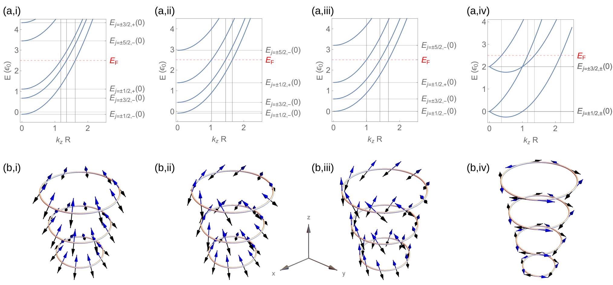
where $\mathcal{J}_{z}\psi_{j,\pm}=\hbar\,j\psi_{j,\pm}$ and with an appropriate normalization constant $\mathcal{N}\equiv\braket{\psi_{j,\pm}(k_{z})|\psi_{j,\pm}(k_{z})}$. Both states $\psi_{j,+}$ and $\psi_{j,-}$ have the same total angular momentum quantum number but different energy as they originate from different orbital angular momenta and spin quantum numbers. In accordance with time-reversal symmetry, the eigenenergies are degenerate with respect to the inversion of $j$ and $k_{z}$. An additional degeneracy appears if $f_{j}(k_{z})=0$, which happens for $\xi=k_{z}=0$ and $\alpha=-\epsilon_{0}R$. The eigenenergies for the lowest subbands are shown in Fig. 2(a,i-iv) for different values of the SOC strengths.

There exist cases in which the eigenvectors can be further factorized into an orbital and a spinor part where the latter does no more depend on the magnitude of the wave vector. In the quantum ring, this is trivially given since the wave vector $k_{z}$ is essentially absent in the SOC terms. On the contrary, in the quantum tube, there are two peculiar situations in which this can be realized. (i) For $\xi=0$ and $\alpha=-\epsilon_{0}R$, the eigenvectors can be factorized as

where the spinors depend only on the sign of $k_{z}$, i.e.,

(ii) Similarly, for $\alpha=0$, the corresponding eigenspinor depends only on the sign of $j$ and reads as

to be evaluated at $\alpha=0$, which is, thus, independent of $k_{z}$. [Eq. (25) also represents the eigenspinor for the quantum ring when setting $k_{z}=0$ and $\alpha$ can be arbitrary.] In each of these cases, the spinor has the property $\chi_{\text{sgn}(k_{z})}^{\pm}=\chi_{\text{sgn}(-k_{z})}^{\mp}$ or $\chi_{\text{sgn}(j)}^{\pm}=\chi_{\text{sgn}(-j)}^{\mp}$, respectively. As it becomes clear later in Sec. III.1, in both situations the corresponding spin states constitute a constant of motion. The disentanglement of the spin and orbital part in the eigenfunctions is one essential feature thereof. Another important observation is that in the above-mentioned cases (i) and (ii) the energy gap between certain subbands becomes independent of the wave vector $k_{z}$, which is generically valid in the absence of SOC. We address this in more detail in Sec. V, where we demonstrate this property leads to distinctive features in the optical conductivity spectrum.

We can account for the effect of a homogeneous magnetic field on the orbital motion of the electrons by minimal coupling $\mathbf{k}\rightarrow\mathbf{k}+\frac{e}{\hbar}\mathbf{A}$ to a vector potential $\mathbf{A}$. For a magnetic field along the symmetry axis, i.e., $\mathbf{B}=B\bm{\hat{z}}$, the vector potential can be chosen as $\mathbf{A}={}(BR/2)\bm{\hat{\phi}}$. In the effective Hamiltonian for the quantum tube and ring, this yields a replacement of the (unit-less) angular momentum operator $l_{z}\rightarrow l_{z}+\Phi/\Phi_{0}$, where $\Phi=BR^{2}\pi$ denotes the magnetic flux and $\Phi_{0}=h/e$ the flux quantum. For large magnetic fields, the Zeeman term should be also taken into account. Neglecting the Zeeman term, the eigensystem is equivalent to the one defined in Sec. II.5 when replacing $j\rightarrow j+\Phi/\Phi_{0}$ apart from the exponent in the eigenvectors. Correspondingly, the energies are degenerate with respect to the substitution $j+\Phi/\Phi_{0}\leftrightarrow-j-\Phi/\Phi_{0}$. The implications of the axial magnetic field are discussed in Sec. IV in view of spontaneously emerging persistent charge and spin currents in the quantum tube and ring.

The time evolution of a general spin quantity $\Sigma$ follows the Heisenberg equation ${\rm d}\Sigma/{\rm d}t=\frac{i}{\hbar}[\mathcal{H},\Sigma]$. In the case that the commutator vanishes, $\Sigma$ describes a constant of motion.

The local spin expectation values $\braket{\mathbf{s}}_{j,\pm}(k_{z})$ of an eigenstates $\psi_{j,\pm}(k_{z})$ are given by $\mathbf{s}_{j,\pm}(k_{z})=\frac{\hbar}{2}\braket{\bm{\sigma}}_{j,\pm}(k_{z})$, where the vector $\braket{\bm{\sigma}}_{j,\pm}(k_{z})=\braket{\psi_{j,\pm}(k_{z})|\bm{\sigma}|\psi_{j,\pm}(k_{z})}$ describes the local spin orientation. The global spin expectation value $\braket{\mathbf{S}}_{j,\pm}(k_{z})$ can be obtained by averaging over the periphery $\phi$, i.e., $\braket{\mathbf{S}}_{j,\pm}(k_{z})=\int_{0}^{2\pi}{\rm d}\phi\,\braket{\mathbf{s}}_{j,\pm}(k_{z})/(2\pi)$. Due to the axial symmetry of the SOC, the radial and tangential components of the global spin expectation value vanish and the $z$-component is identical with the local spin expectation value.

The components of the charge ($c$) and spin ($s$) current density operators $\mathbf{j}^{c/s}$ are defined asSheng and Chang 2006; Sun et al. 2008

where $e>0$ is the elementary charge, $v_{n}$ is the $n$th component of the velocity operator $\mathbf{v}=\frac{i}{\hbar}[\mathcal{H},\mathbf{r}]$, and the anti-commutator ensures the result being real valued. For a given normalized state $\Psi(\mathbf{r})$ the current density expectation values become

The state-dependent charge or spin current through a cross-section $\mathcal{A}$ (given by integration over the area element ${\rm d}\bm{\mathcal{A}}$) is obtained viaSplettstoesser et al. 2003

To obtain the total current $I^{c/s}_{n,(q)}$, we need to sum the respective state-dependent counterpart over all occupied states. Here, we can encounter two different physical situations in experiment.Kokurin 2018 (I) The quantum structure is isolated and contains a fixed particle number. As a result, the currents are distinct for even or odd particle numbers.Splettstoesser et al. 2003 The flux-dependent jumps appear at the energy-level crossings with the same spin orientation. (II) The quantum structure is coupled to a reservoir, which yields a constant chemical potential (or Fermi energy at zero temperature). Here, the particle number is irrelevant and the flux-dependent jumps appear at the intersections of energy levels with the chemical potential. In this work, we focus on the situation (II).

In the tubular system, the azimuthal and axial velocity components are given by

For an eigenstate $\psi_{j,\pm}(k_{z})$, we obtain for the expectation value of the charge current densities

and the spin current densities

with

the effective volume of the quantum tube $\mathcal{V}=2\pi RL$, and we suppressed the argument $(k_{z})$ in the current density for compactness. The axial and azimuthal spin current density tensor components $\braket{j^{s}_{z,q}}_{j,\pm}$ and $\braket{j^{s}_{\phi,q}}_{j,\pm}$ for $q\in\{r,\phi,z\}$ show analogous behaviour as the local spin orientation with respect to the SOC parameters, meaning that, the $r$-component vanishes for $\xi=0$, the $\phi$-component vanishes for $\alpha=0$, and the $z$-component vanishes for $\alpha=-\epsilon_{0}R$. The inclusion of an axial magnetic field requires the substitution $j\rightarrow j+\Phi/\Phi_{0}$ in the expressions for the current densities (cf. Sec. II.6).

At zero temperature, the total equilibrium current $I^{c/s}_{n,(q)}$ is obtained by summing over all states below the Fermi energy, that is,

where $\Theta$ denotes the Heaviside function and we have $\mathcal{A}_{\phi}=L$ for an azimuthal current and $\mathcal{A}_{z}=2\pi R$ for an axial current. The $k_{z}$ mirror-symmetry of the eigenenergies implies that only current density components that are even in $k_{z}$ remain, i.e., $\braket{j^{c}_{\phi}}_{j,\pm}$ for the charge current density and $\braket{j^{s}_{z,\phi}}_{j,\pm}$, $\braket{j^{s}_{\phi,r}}_{j,\pm}$, and $\braket{j^{s}_{\phi,z}}_{j,\pm}$ for the spin current density. The same holds for the $j$-summation unless the axial magnetic field is present. Hence, if the magnetic field is zero, the total equilibrium charge current vanishes in agreement with time-reversal symmetry. On the contrary, the spin current is non-zero even in absence of the magnetic field as it results from space-inversion symmetry breaking. The contributing terms are the same as without magnetic field.

In the case of a quantum ring, the above expressions for the azimuthal current densities remain valid if we set $k_{z}=0$ and identify the effective volume as the circumference of the ring, i.e., $\mathcal{V}=2\pi R$. The total azimuthal current at zero temperature is given by $I^{c/s}_{\phi,(q)}=\sum_{j,\pm}(I^{c/s}_{\phi,(q)})_{j,\pm}\Theta[E_{\text{F}}-E_{j,\pm}]$ where $(I^{c/s}_{\phi,(q)})_{j,\pm}=\braket{j^{c/s}_{\phi,(q)}}_{j,\pm}$. Equivalently, for a non-vanishing axial magnetic field, we can also utilize the formulasSplettstoesser et al. 2003

with the eigenenergies and local spin orientations of the quantum ring (cf. Secs. II.5 and III.2).

We demonstrate now that both physical systems, quantum tube and quantum ring, show characteristic features of the bandstructure in the current dependence on the Fermi energy as well as the magnetic flux. While the changes in the currents occur rapidly for the ring, the continuous energy branches of the quantum tube yield smoother variations. The fingerprints result from the underlying band structure where, interestingly, the critical energies or magnetic fluxes are identical in the tube and the ring. Apparently, in the quantum tube, the characteristics are determined by the band structure at $k_{z}=0$, which coincides with the (discrete) energy levels of the quantum ring. These commonalities allow us to point out general relations that hold for both systems at the same time. For simplification, we assume $\xi=\tilde{\xi}$ in the following.

We start by discussing the case without a magnetic field, where only spin currents remain. In such an experimental situation, the modulation of physical parameters is focused on SOC coefficients and Fermi energy, where the latter conforms to the carrier density. In Fig. 3, we demonstrate the dependence of the spin currents on the Fermi energy for the quantum ring (a) and the quantum tube [(b),(c)]. For the latter, we ignored for the small dependence of $\xi$ on the Fermi energy. In Fig. 3(d), the respective energy dispersion for the quantum tube is shown, where the vertical grid lines emphasize the subband minima $E_{j,\pm}(k_{z}=0)$ [cf. Eq. (20)]. Kinks appear when the Fermi energy surpasses an eigenenergy value $E_{j,\pm}(k_{z}=0)$ of the quantum tube, or, equivalently, an energy level of the quantum ring.

Now, we turn to the persistent charge and spin current dependence on the magnetic flux. An example is given in Fig. 4 together with the corresponding flux dependence of the energy spectrum at $k_{z}=0$. Primarily, the structure of the currents is $\Phi_{0}$-periodic. In the energy spectrum, Fig. 4(f), we find this periodicity in the neighboring branches with the same slope. Within one period we recognize several substructures, where the energy-levels intersect with the Fermi energy. The jumps or kinks depend, on the one hand, on the magnitude of the Fermi energy, on the other hand, on the SOC strength. For a given Fermi energy $E_{\text{F}}$ they occur at

with any combination of the occurring signs and $u\in\mathbb{Z}$ accounting for the $\Phi_{0}$ periodicity. In the special situation that $\xi=0$ and $\alpha=-\epsilon_{0}R$ [PSH case (i)], the eigenenergies $E_{j,\pm}(k_{z}=0)$ are degenerate and the critical flux values associated with the different signs of the last term in Eq. (53) become identical.

With regard to the spin currents, we find that generally only the tensor components $I^{s}_{\phi,r},I^{s}_{\phi,z}$, and $I^{s}_{z,\phi}$ are allowed. Apart from this, we obtain the following special cases depending on the SOC coefficients holding for both quantum structures with or without magnetic flux if applicable. (i) For $\xi=0$ and $\alpha=-\epsilon_{0}R$ all spin currents vanish. (ii) For $\alpha=0$, the $\phi$-component is zero, i.e., $I^{s}_{z,\phi}=0$. (iii) For $\alpha=-\epsilon_{0}R$, the $z$-component is zero, i.e., $I^{s}_{\phi,z}=0$. (iv) For $\xi=0$, the $r$-component is zero, i.e., $I^{s}_{\phi,r}=0$. [Notice that (i) and (ii) correspond to the PSH case in the quantum tube.]

We conclude that the sudden changes in the persistent currents with respect to the modulation of the Fermi energy or the magnetic flux are directly related to characteristics of the electronic band structure. These signatures are visible in the quantum ring as well as the quantum tube and allow to extract band parameters such as SOC strengths. The PSH symmetries (i) and (ii) of the quantum tube become manifest in the vanishing of spin current tensor components. The PSH case (i) exhibits also flux-dependent features due to the additional band degeneracy at vanishing wave vectors.

The application of a time-dependent weak electric field $\delta\bm{\mathcal{E}}(t)$ generates a contribution $\delta\bm{j}(t)$ to the charge current density. Within linear response theory, the frequency-dependent optical conductivity tensor $\sigma_{\mu\nu}(\omega)$ relates the Fourier-transformed AC quantities [current density $\delta j_{\mu}(\omega)$ and electric field $\delta\mathcal{E}_{\nu}(\omega)$] via the linear relation ${\delta j_{\mu}(\omega)=\sigma_{\mu\nu}(\omega)\,\delta\mathcal{E}_{\nu}(\omega)}$.

The Kubo formula for a generic conductivity tensor $\sigma_{\mu\nu}$ as linear response to a spatially homogeneous AC electric field $\delta\bm{\mathcal{E}}(t)=\lim_{\eta\to 0^{+}}\delta\bm{\mathcal{E}}(\omega)\exp[-i(\omega+i\eta)t]$ is expressed in terms of the set of single-particle eigenstates $\{\ket{n}\}$. In the frequency domain it reads as Kammermeier 2018; Kammermeier et al. 2019

with the volume $\mathcal{V}$, the components of the velocity operator v, and the single-particle eigenenergies $\epsilon_{n}$. The function $f(\epsilon_{n})=\{1+\exp[\beta(\epsilon_{n}-\tilde{\mu})]\}^{-1}$, where $\beta=1/(k_{B}T)$, represents the Fermi-Dirac distribution with the Boltzmann constant $k_{B}$, the temperature $T$, and the chemical potential $\tilde{\mu}$. Here, one usually distinguishes an intra-band ($n=l$) contribution, which determines the DC Drude conductivity, and an inter-band ($n\neq l$) contribution, which determines the optical absorption at finite frequencies. The effect of disorder can be incorporated by replacing $\eta\rightarrow\hbar/(2\tau_{\text{p}})$ with the finite momentum relaxation time $\tau_{\text{p}}$. We are interested in the dissipative part, which is given by the real part of the conductivity tensor $\text{Re}\left[\sigma_{\mu\nu}(\omega)\right]$.

Although the optical conductivity has been studied in numerous different contexts, there exist only few studies that focus on nanowires. For instance, Ref. Kurbatsky and Pogosov 2010 studies the effect of size-quantization on the optical conductivity in metallic wires and Refs. Khordad 2013; Winkler et al. 2017 discusses the impact of the interplay between a magnetic field and Rashba SOC on the optical properties in 1D or quasi-1D wires. Here, we neglect magnetic field effects and focus on the emergence of features in the optical conductivity that arise from the PSH symmetry in the tubular nanowires. These are described by the quasi-2D quantum tube Hamiltonian with the eigenenergies $E_{j,\pm}(k_{z})$ and according eigenstates $\psi_{j,\pm}(k_{z})$ (cf. Sec. II.5).

Considering an AC-biased nanowire, the AC electric field $\delta\mathcal{E}_{z}(t)$ along the nanowire $z$-axis leads to a dissipative AC charge current density $\delta j_{z}(t)$ described by the longitudinal tensor component $\text{Re}\left[\sigma_{zz}(\omega)\right]$ in the clean limit, i.e. $\tau_{\text{p}}\rightarrow\infty$, as

References

- D’yakonov and Perel’ (1972) M. I. D’yakonov and V. I. Perel’, Sov. Phys. Solid State 13, 3023 (1972), [Fiz. Tverd. Tela 13, 3581 (1971)].
- Schliemann (2017) J. Schliemann, Rev. Mod. Phys. 89, 011001 (2017).
- Kohda and Salis (2017) M. Kohda and G. Salis, Semicond. Sci. Technol. 32, 073002 (2017).
- Schliemann et al. (2003) J. Schliemann, J. C. Egues, and D. Loss, Phys. Rev. Lett. 90, 146801 (2003).
- Bernevig et al. (2006) B. A. Bernevig, J. Orenstein, and S.-C. Zhang, Phys. Rev. Lett. 97, 236601 (2006).
- Trushin and Schliemann (2007) M. Trushin and J. Schliemann, New J. Phys. 9, 346 (2007).
- Sacksteder and Bernevig (2014) V. E. Sacksteder and B. A. Bernevig, Phys. Rev. B 89, 161307(R) (2014).
- Dollinger et al. (2014) T. Dollinger, M. Kammermeier, A. Scholz, P. Wenk, J. Schliemann, K. Richter, and R. Winkler, Phys. Rev. B 90, 115306 (2014).
- Wenk et al. (2016) P. Wenk, M. Kammermeier, and J. Schliemann, Phys. Rev. B 93, 115312 (2016).
- Kammermeier et al. (2016a) M. Kammermeier, P. Wenk, and J. Schliemann, Phys. Rev. Lett. 117, 236801 (2016a).
- Mal’shukov and Chao (2000) A. G. Mal’shukov and K. A. Chao, Phys. Rev. B 61, R2413 (2000).
- Kiselev and Kim (2000) A. A. Kiselev and K. W. Kim, Phys. Rev. B 61, 13115 (2000).
- Schwab et al. (2006) P. Schwab, M. Dzierzawa, C. Gorini, and R. Raimondi, Phys. Rev. B 74, 155316 (2006).
- Th. Schäpers et al. (2006) Th. Schäpers, V. A. Guzenko, M. G. Pala, U. Zülicke, M. Governale, J. Knobbe, and H. Hardtdegen, Phys. Rev. B 74, 081301(R) (2006).
- Kunihashi et al. (2009) Y. Kunihashi, M. Kohda, and J. Nitta, Phys. Rev. Lett. 102, 226601 (2009).
- Kettemann (2007) S. Kettemann, Phys. Rev. Lett. 98, 176808 (2007).
- Wenk and Kettemann (2010) P. Wenk and S. Kettemann, Phys. Rev. B 81, 125309 (2010).
- Wenk and Kettemann (2011) P. Wenk and S. Kettemann, Phys. Rev. B 83, 115301 (2011).
- Kammermeier et al. (2017) M. Kammermeier, P. Wenk, J. Schliemann, S. Heedt, Th. Gerster, and Th. Schäpers, Phys. Rev. B 96, 235302 (2017).
- Kammermeier et al. (2018) M. Kammermeier, P. Wenk, F. Dirnberger, D. Bougeard, and J. Schliemann, Phys. Rev. B 98, 035407 (2018).
- Dirnberger et al. (2019) F. Dirnberger, M. Kammermeier, J. König, M. Forsch, P. E. Faria Junior, T. Campos, J. Fabian, J. Schliemann, C. Schüller, T. Korn, P. Wenk, and D. Bougeard, Appl. Phys. Lett. 114, 202101 (2019).
- Abrahams et al. (1979) E. Abrahams, P. W. Anderson, D. C. Licciardello, and T. V. Ramakrishnan, Phys. Rev. Lett. 42, 673 (1979).
- Moroz et al. (2000) A. V. Moroz, K. V. Samokhin, and C. H. W. Barnes, Phys. Rev. Lett. 84, 4164 (2000).
- Gritsev et al. (2005) V. Gritsev, G. I. Japaridze, M. Pletyukhov, and D. Baeriswyl, Phys. Rev. Lett. 94, 137207 (2005).
- Gray et al. (2015) F. S. Gray, T. Kernreiter, M. Governale, and U. Zülicke, Phys. Rev. B 92, 115414 (2015).
- Yang et al. (2010) P. Yang, R. Yan, and M. Fardy, Nano Lett. 10, 1529 (2010).
- Nadj-Perge et al. (2010) S. Nadj-Perge, S. M. Frolov, E. P. A. M. Bakkers, and L. P. Kouwenhoven, Nature 468, 1084 (2010).
- Nadj-Perge et al. (2012) S. Nadj-Perge, V. S. Pribiag, J. W. G. van den Berg, K. Zuo, S. R. Plissard, E. P. A. M. Bakkers, S. M. Frolov, and L. P. Kouwenhoven, Phys. Rev. Lett. 108, 166801 (2012).
- Frolov et al. (2013) S. M. Frolov, S. R. Plissard, S. Nadj-Perge, L. P. Kouwenhoven, and E. P. Bakkers, MRS Bulletin 38, 809–815 (2013).
- Heedt et al. (2013) S. Heedt, I. Wehrmann, K. Weis, R. Calarco, H. Hardtdegen, D. Grützmacher, Th. Schäpers, C. Morgan, and D. E. Bürgler, “Toward spin electronic devices based on semiconductor nanowires,” in Future Trends in Microelectronics (John Wiley & Sons, Inc., 2013) pp. 328–339.
- Krogstrup et al. (2013) P. Krogstrup, H. I. Jørgensen, M. Heiss, O. Demichel, J. V. Holm, M. Aagesen, J. Nygård, and A. Fontcuberta i Morral, Nat. Photonics 7, 306 (2013).
- Dai et al. (2014) X. Dai, S. Zhang, Z. Wang, G. Adamo, H. Liu, Y. Huang, C. Couteau, and C. Soci, Nano Lett. 14, 2688 (2014).
- Faria Junior et al. (2015) P. E. Faria Junior, G. Xu, J. Lee, N. C. Gerhardt, G. M. Sipahi, and I. Žutić, Phys. Rev. B 92, 075311 (2015).
- Dai et al. (2015) X. Dai, A. Messanvi, H. Zhang, C. Durand, J. Eymery, C. Bougerol, F. H. Julien, and M. Tchernycheva, Nano Lett. 15, 6958 (2015).
- Goktas et al. (2018) N. I. Goktas, P. Wilson, A. Ghukasyan, D. Wagner, S. McNamee, and R. R. LaPierre, Appl. Phys. Rev. 5, 041305 (2018).
- Shadi A. Dayeh (2016) C. J. Shadi A. Dayeh, Anna Fontcuberta i Morral, ed., Semiconductor Nanowires II: Properties and Applications (Elsevier, Academic Press, Amsterdam, 2016).
- Fortuna and Li (2010) S. A. Fortuna and X. Li, Semicond. Sci. Technol. 25, 024005 (2010).
- Glas et al. (2007) F. Glas, J.-C. Harmand, and G. Patriarche, Phys. Rev. Lett. 99, 146101 (2007).
- Krogstrup et al. (2011) P. Krogstrup, S. Curiotto, E. Johnson, M. Aagesen, J. Nygård, and D. Chatain, Phys. Rev. Lett. 106, 125505 (2011).
- Rieger et al. (2013) T. Rieger, M. I. Lepsa, Th. Schäpers, and D. Grützmacher, J. Cryst. Growth 378, 506 (2013).
- Schroth et al. (2015) P. Schroth, M. Köhl, J.-W. Hornung, E. Dimakis, C. Somaschini, L. Geelhaar, A. Biermanns, S. Bauer, S. Lazarev, U. Pietsch, and T. Baumbach, Phys. Rev. Lett. 114, 055504 (2015).
- Fontcuberta i Morral (2016) A. Fontcuberta i Morral, Nature 531, 308 (2016).
- Jacobsson et al. (2016) D. Jacobsson, F. Panciera, J. Tersoff, M. C. Reuter, S. Lehmann, S. Hofmann, K. A. Dick, and F. M. Ross, Nature 531, 317 (2016).
- De and Pryor (2010) A. De and C. E. Pryor, Phys. Rev. B 81, 155210 (2010).
- Cheiwchanchamnangij and Lambrecht (2011) T. Cheiwchanchamnangij and W. R. L. Lambrecht, Phys. Rev. B 84, 035203 (2011).
- Gmitra and Fabian (2016) M. Gmitra and J. Fabian, Phys. Rev. B 94, 165202 (2016).
- Campos et al. (2018) T. Campos, P. E. Faria Junior, M. Gmitra, G. M. Sipahi, and J. Fabian, Phys. Rev. B 97, 245402 (2018).
- Faria Junior et al. (2016) P. E. Faria Junior, T. Campos, C. M. O. Bastos, M. Gmitra, J. Fabian, and G. M. Sipahi, Phys. Rev. B 93, 235204 (2016).
- Faria Junior et al. (2019) P. E. Faria Junior, D. Tedeschi, M. De Luca, B. Scharf, A. Polimeni, and J. Fabian, Phys. Rev. B 99, 195205 (2019).
- Fu et al. (2020) J. Fu, P. H. Penteado, D. R. Candido, G. J. Ferreira, D. P. Pires, E. Bernardes, and J. C. Egues, Phys. Rev. B 101 (2020).
- Luo et al. (2020) J.-W. Luo, S.-S. Li, and A. Zunger, (2020), arXiv:2003.02984 .
- Intronati et al. (2013) G. A. Intronati, P. I. Tamborenea, D. Weinmann, and R. A. Jalabert, Phys. Rev. B 88, 045303 (2013).
- Scherübl et al. (2016) Z. Scherübl, G. Fülöp, M. H. Madsen, J. Nygård, and S. Csonka, Phys. Rev. B 94, 035444 (2016).
- Jespersen et al. (2018) T. S. Jespersen, P. Krogstrup, A. M. Lunde, R. Tanta, T. Kanne, E. Johnson, and J. Nygård, Phys. Rev. B 97, 041303(R) (2018).
- Iorio et al. (2019) A. Iorio, M. Rocci, L. Bours, M. Carrega, V. Zannier, L. Sorba, S. Roddaro, F. Giazotto, and E. Strambini, Nano Lett. 19, 652 (2019).
- Furthmeier et al. (2016) S. Furthmeier, F. Dirnberger, M. Gmitra, A. Bayer, M. Forsch, J. Hubmann, C. Schüller, E. Reiger, J. Fabian, T. Korn, and D. Bougeard, Nat. Commun. 7, 12413 (2016).
- Buß et al. (2019) J. H. Buß, S. Fernández-Garrido, O. Brandt, D. Hägele, and J. Rudolph, Appl. Phys. Lett. 114, 092406 (2019).
- Estévez Hernández et al. (2010) S. Estévez Hernández, M. Akabori, K. Sladek, C. Volk, S. Alagha, H. Hardtdegen, M. G. Pala, N. Demarina, D. Grützmacher, and Th. Schäpers, Phys. Rev. B 82, 235303 (2010).
- Hyun et al. (2013) J. K. Hyun, S. Zhang, and L. J. Lauhon, Annu. Rev. Mater. Res. 43, 451 (2013).
- Degtyarev et al. (2017) V. E. Degtyarev, S. V. Khazanova, and N. V. Demarina, Sci. Rep. 7, 3411 (2017).
- Haas et al. (2017) F. Haas, P. Zellekens, M. Lepsa, T. Rieger, D. Grützmacher, H. Lüth, and T. Schäpers, Nano Lett. 17, 128 (2017).
- Corfdir et al. (2019) P. Corfdir, O. Marquardt, R. B. Lewis, C. Sinito, M. Ramsteiner, A. Trampert, U. Jahn, L. Geelhaar, O. Brandt, and V. M. Fomin, Adv. Mater. 31, 1805645 (2019).
- Zellekens et al. (2020) P. Zellekens, N. Demarina, J. Janßen, T. Rieger, M. I. Lepsa, P. Perla, G. Panaitov, H. Lueth, D. Gruetzmacher, and T. Schäpers, Semicond. Sci. Technol. (2020).
- Bringer and Th. Schäpers (2011) A. Bringer and Th. Schäpers, Phys. Rev. B 83, 115305 (2011).
- Kokurin (2015) I. Kokurin, Phys. E 74, 264 (2015).
- Kammermeier et al. (2016b) M. Kammermeier, P. Wenk, J. Schliemann, S. Heedt, and Th. Schäpers, Phys. Rev. B 93, 205306 (2016b).
- Zellekens et al. (2019) P. Zellekens, N. Demarina, J. Janßen, T. Rieger, M. I. Lepsa, P. Perla, G. Panaitov, H. Lüth, D. Grützmacher, and Th. Schäpers, (2019), arXiv:1911.05510 .
- Lahiri et al. (2018) A. Lahiri, K. Gharavi, J. Baugh, and B. Muralidharan, Phys. Rev. B 98, 125417 (2018).
- Li et al. (2013) Z. Li, F. Marsiglio, and J. P. Carbotte, Sci. Rep. 3, 2828 (2013).
- Büttiker et al. (1983) M. Büttiker, Y. Imry, and R. Landauer, Phys. Lett. A 96, 365 (1983).
- Splettstoesser et al. (2003) J. Splettstoesser, M. Governale, and U. Zülicke, Phys. Rev. B 68, 165341 (2003).
- Sheng and Chang (2006) J. S. Sheng and K. Chang, Phys. Rev. B 74, 235315 (2006).
- Sun et al. (2007) Q.-f. Sun, X. C. Xie, and J. Wang, Phys. Rev. Lett. 98, 196801 (2007).
- Sun et al. (2008) Q.-f. Sun, X. C. Xie, and J. Wang, Phys. Rev. B 77, 035327 (2008).
- Kokurin (2018) I. A. Kokurin, Semicond. 52, 535 (2018).
- Fu and Wu (2008) J. Y. Fu and M. W. Wu, J. Appl. Phys. 104, 093712 (2008).
- Zutic et al. (2004) I. Zutic, J. Fabian, and S. Das Sarma, Rev. Mod. Phys. 76, 323 (2004).
- Liang and Gao (2012) D. Liang and X. P. Gao, Nano Lett. 12, 3263 (2012).
- Bringer et al. (2019) A. Bringer, S. Heedt, and Th. Schäpers, Phys. Rev. B 99, 085437 (2019).
- Kammermeier (2018) M. Kammermeier, Control of Spin Relaxation in Disordered Quantum Wells and Nanowires, Ph.D. thesis, University of Regensburg (2018).
- Meijer et al. (2002) F. E. Meijer, A. F. Morpurgo, and T. M. Klapwijk, Phys. Rev. B 66, 033107 (2002).
- Berche et al. (2010) B. Berche, C. Chatelain, and E. Medina, Eur. J. Phys. 31, 1267 (2010).
- Durnev et al. (2014) M. V. Durnev, M. M. Glazov, and E. L. Ivchenko, Phys. Rev. B 89, 075430 (2014).
- Simion and Lyanda-Geller (2014) G. E. Simion and Y. B. Lyanda-Geller, Phys. Rev. B 90, 195410 (2014).
- (85) Note that in App. D of Ref. \rev@citealpnumKammermeier2016, we showed that the precise structure of the radial confining potential V(r) is irrelevant to obtain for the lowest bound state the general relation . Yet, in the proof, we incorrectly state that the operator is Hermitian. Instead, only the sum must be Hermitian. We give the correct solution in App. C.
- Kohda et al. (2012) M. Kohda, V. Lechner, Y. Kunihashi, T. Dollinger, P. Olbrich, C. Schönhuber, I. Caspers, V. V. Bel’kov, L. E. Golub, D. Weiss, K. Richter, J. Nitta, and S. D. Ganichev, Phys. Rev. B 86, 081306(R) (2012).
- Schliemann et al. (2006) J. Schliemann, D. Loss, and R. M. Westervelt, Phys. Rev. B 73, 085323 (2006).
- Badalyan et al. (2009) S. M. Badalyan, A. Matos-Abiague, G. Vignale, and J. Fabian, Phys. Rev. B 79, 205305 (2009).
- Shen (2004) S.-Q. Shen, Phys. Rev. B 70, 081311(R) (2004).
- Sinitsyn et al. (2004) N. A. Sinitsyn, E. M. Hankiewicz, W. Teizer, and J. Sinova, Phys. Rev. B 70, 081312(R) (2004).
- Kammermeier et al. (2019) M. Kammermeier, P. Wenk, and U. Zülicke, Phys. Rev. B 100, 075421 (2019).
- Kurbatsky and Pogosov (2010) V. P. Kurbatsky and V. V. Pogosov, Phys. Rev. B 81, 155404 (2010).
- Khordad (2013) R. Khordad, J. Lumin. 134, 201 (2013).
- Winkler et al. (2017) G. W. Winkler, M. Ganahl, D. Schuricht, H. G. Evertz, and S. Andergassen, New J. Phys. 19, 063009 (2017).
- Cruz et al. (2018) E. Cruz, C. López-Bastidas, and J. A. Maytorena, J. Appl. Phys. 123, 113902 (2018).