跳到论文正文
W Papers独立论文阅读器 arXiv:2001.06562 论文正文 计算阅读时间 · 0%
引用这篇论文根据当前论文元数据生成,正式投稿前建议核对。


License: arXiv.org perpetual non-exclusive license
arXiv:2001.06562v2 [eess.SY] 26 Sep 2020

Set-Membership Filter for Discrete-Time Nonlinear Systems Using State Dependent Coefficient Parameterization

Diganta Bhattacharjee and Kamesh Subbarao    Thanks: D. Bhattacharjee and K. Subbarao are with the Department of Mechanical and Aerospace Engineering, The University of Texas at Arlington, Arlington, TX, 76019 USA e-mail: diganta.bhattacharjee@mavs.uta.edu, subbarao@uta.edu
Abstract

In this technical note, a recursive set-membership filtering algorithm for discrete-time nonlinear dynamical systems subject to unknown but bounded process and measurement noises is proposed. The nonlinear dynamics is represented in a pseudo-linear form using the state dependent coefficient (SDC) parameterization. Matrix Taylor expansions are utilized to expand the state dependent matrices about the state estimates. Upper bounds on the norms of remainders in the matrix Taylor expansions are calculated on-line using a non-adaptive random search algorithm at each time step. Utilizing these upper bounds and the ellipsoidal set description of the uncertainties, a two-step filter is derived that utilizes the ‘correction-prediction’ structure of the standard Kalman Filter variants. At each time step, correction and prediction ellipsoids are constructed that contain the true state of the system by solving the corresponding semi-definite programs (SDPs). Finally, a simulation example is included to illustrate the effectiveness of the proposed approach.

Index Terms: 
Set-membership filtering, bounding ellipsoids, unknown but bounded noise, state dependent coefficient parameterization.

I Introduction

A broad class of state estimation and filtering approaches require stochastic description of the process noise corrupting the state of the system and the noise associated with the measurements, e.g., Kalman Filters are optimal for linear systems with uncorrelated, Gaussian process and measurement noises [1]. An alternative approach involves assuming the noises to be unknown but bounded. Under this assumption, the solution to the estimation problem requires set of states consistent with the knowledge of the bounds on the noises, the governing equations or models, and the measurements [2, 3]. This approach is generally referred to as set-membership, set-valued, guaranteed estimation or filtering [4, 5, 2, 3, 6, 7, 8] and was introduced in the late 1960s and early 1970s [9, 10, 11]. As the actual set containing all possible values of the state is, in general, very complex and hard to obtain, several approximations (ellipsoids, polytopes, zonotopes) have been studied in the literature.

In this technical note, the ellipsoidal state estimation problem is considered and the terminology set-membership filter (SMF) is adopted. Over the years, set-membership filtering for linear systems has attracted significant attention and the theory is well-established (see, e.g., [5, 3, 6] and the references therein). Particularly, the filter design proposed in this technical note is motivated by [5, 6] where the set estimation problems were converted into recursive algorithms that require solutions to semi-definite programs (SDPs) at each time step. Recently, several extensions of this approach have emerged in the literature (see, e.g.,[12, 13, 14]).

On the other hand, set-membership filtering for discrete-time nonlinear systems has received less attention. For discrete-time nonliner systems, similar to the Extended Kalman Filter (EKF), set-membership filtering approaches typically involve linearizing the nonlinear dynamics about the state estimate trajectory [15, 16, 8, 13]. An extended set-membership filter (ESMF) was developed in [15] by linearizing the state dynamics about the state estimates and bounding the linearization errors using interval analysis. An improvement over the algorithm proposed in [15] was provided in [16]. The SDP-based approach for discrete-time nonlinear systems was introduced in [8] with a prediction-correction form. Recently, this approach was extended in [13] where the linearization errors were bounded by ellipsoids on-line.

Alternatively, state dependent coefficient (SDC) parameterization can be utilized to represent a nonlinear system in a pseudo-linear form with state dependent system matrices [17, 18]. The parameterization is non-unique and the non-uniqueness can be utilized to enhance performance of the controller or filter design (see, e.g., [18, 19]). SDC parameterization has been utilized for filter design in a stochastic framework for discrete-time nonlinear systems (see [20, 21]). However, set-membership filtering using the SDC parameterization has not been addressed in the existing open literature to the best of the authors’ knowledge.

Motivated by the above discussion, a recursive SMF utilizing the SDC parameterization (SDC-SMF) is proposed in this technical note for discrete-time nonlinear systems subject to unknown but bounded process and measurement noises. A two-step correction-prediction form is developed, similar to the Kalman Filter variants [1]. The proposed filter requires solutions to two SDPs at each time step, similar to [8, 13]. The technical novelties of the proposed approach are three fold and are summarized as follows.

  1. 1.

    A single SDC parameterization of the nonlinear system is utilized to obtain a pseudo-linear representation which preserves the nonlinearity in the governing equations. To the best of our knowledge, this is the first SMF for discrete-time nonlinear systems that utilizes the SDC parameterization.

  2. 2.

    Instead of taking the EKF-like approach for SMF frameworks as in [15, 8, 16, 13], the state dependent matrices are expanded about the state estimates in matrix Taylor expansions using Vetter calculus [22]. Upper bounds on the norms of remainders in the matrix Taylor expansions are calculated on-line at each time step and those bounds are utilized in the filter design at every recursion. This approach is different from the approaches in [15, 16] where interval analysis were utilized to bound the linearization errors and from the recent approach in [13] where the linearization errors were bounded by ellipsoidal sets.

  3. 3.

    We make use of predefined structures for the state estimates which are similar to the traditional Kalman filtering technique. However, this is unlike the SDP-based SMFs for discrete-time nonlinear systems in [8, 13] where the state estimates constitute a part of the optimization variables.

Our approach of dealing with the remainders is computationally cheaper compared to the ellipsoidal bounding methodology in [13] which requires additional SDPs to be solved, increasing the associated computational cost. Also, the above technical novelties lead to better filtering performance compared to the framework in [13], as demonstrated in the simulation results. The rest of this technical note is organized as follows. Section II describes the preliminaries and problem formulation for the SDC-SMF. Section III discusses the main results for the proposed SDC-SMF and formulates the SDPs to be solved at each time step to find the ellipsoidal sets containing the true state of the system. Finally, Section V includes a simulation example and Section VI presents the concluding remarks.

Notation

The symbol ℤ⋆\mathbb{Z}_{\star} denotes the set of non-negative integers. For a square matrix 𝑿\bm{X}, the notation 𝑿>0\bm{X}>0 (respectively, 𝑿≥0\bm{X}\geq 0) means 𝑿\bm{X} is symmetric and positive definite (respectively, positive semi-definite). Similarly, 𝑿<0\bm{X}<0 (respectively, 𝑿≤0\bm{X}\leq 0) means 𝑿\bm{X} is symmetric and negative definite (respectively, negative semi-definite). The notations diag​(⋅)\text{diag}(\cdot), 𝑰n\bm{I}_{n}, 𝑶n\bm{O}_{n}, and 𝟎n\bm{0}_{n} denote block-diagonal matrices, the n×nn\times n identity matrix, the n×nn\times n null matrix, and the vector of zeros of dimension nn, respectively. The symbol ||⋅||||\cdot|| denotes the spectral norm for matrices and the Euclidean norm for vectors. Ellipsoids are denoted by ℰ⁡(𝒄,𝑷)={𝒙∈ℝn:(𝒙−𝒄)T​𝑷−1​(𝒙−𝒄)≤1}\mathcal{E}(\bm{c},\bm{P})=\{\bm{x}\in\mathbb{R}^{n}:(\bm{x}-\bm{c})^{\text{T}}\bm{P}^{-1}(\bm{x}-\bm{c})\leq 1\} where 𝒄∈ℝn\bm{c}\in\mathbb{R}^{n} is the center of the ellipsoid and 𝑷>0\bm{P}>0 is the shape matrix that characterizes the orientation and size of the ellipsoid in ℝn\mathbb{R}^{n}. Also, the Kronecker product is denoted by ⊗\otimes and a function that is continuously differentiable tt times is said to be of class CtC^{t}. To this end, C0C^{0} denotes the class of continuous functions.

II Preliminaries and Problem Formulation

Consider discrete-time, nonlinear dynamical systems of the form

𝒙k+1=𝒇d​(𝒙k)+𝒘k𝒚k=𝒉d​(𝒙k)+𝒗k\begin{split}\bm{x}_{k+1}&=\bm{f}_{d}(\bm{x}_{k})+\bm{w}_{k}\\ \bm{y}_{k}&=\bm{h}_{d}(\bm{x}_{k})+\bm{v}_{k}\end{split} (1)

where k∈ℤ⋆k\in\mathbb{Z}_{\star}, 𝒙k∈ℝn\bm{x}_{k}\in\mathbb{R}^{n} is the state of the system, 𝒘k∈ℝn\bm{w}_{k}\in\mathbb{R}^{n} is the process noise or input disturbance, 𝒚k∈ℝp\bm{y}_{k}\in\mathbb{R}^{p} is the measured output, and 𝒗k∈ℝp\bm{v}_{k}\in\mathbb{R}^{p} is the measurement noise. We make the following standing assumption on the nonlinear functions 𝒇d:ℝn→ℝn\bm{f}_{d}:\mathbb{R}^{n}\rightarrow\mathbb{R}^{n} and 𝒉d:ℝn→ℝp\bm{h}_{d}:\mathbb{R}^{n}\rightarrow\mathbb{R}^{p}.

Assumption 1

𝒇d​(𝟎n)=𝟎n\bm{f}_{d}(\bm{0}_{n})=\bm{0}_{n}, 𝐡d​(𝟎n)=𝟎p\bm{h}_{d}(\bm{0}_{n})=\bm{0}_{p}, and 𝐟d​(⋅)∈Ct\bm{f}_{d}(\cdot)\in C^{t}, 𝐡d​(⋅)∈Ct\bm{h}_{d}(\cdot)\in C^{t} where t≥2t\geq 2.

Under Assumption 1, the nonlinear functions can be put into corresponding pseudo-linear forms using the SDC parameterization as

𝒇d​(𝒙k)=𝑨⁡(𝒙k)​𝒙k𝒉d​(𝒙k)=𝑯⁡(𝒙k)​𝒙k\begin{split}\bm{f}_{d}(\bm{x}_{k})&=\bm{A}(\bm{x}_{k})\bm{x}_{k}\\ \bm{h}_{d}(\bm{x}_{k})&=\bm{H}(\bm{x}_{k})\bm{x}_{k}\end{split} (2)

where 𝑨:ℝn→ℝn×n\bm{A}:\mathbb{R}^{n}\rightarrow\mathbb{R}^{n\times n} and 𝑯:ℝn→ℝp×n\bm{H}:\mathbb{R}^{n}\rightarrow\mathbb{R}^{p\times n} are nonlinear matrix-valued functions. To this end, we recall the following useful result.

Proposition 1

[18, 23] Under Assumption 1, SDC parameterizations of 𝐟d​(𝐱k),𝐡d​(𝐱k)\bm{f}_{d}(\bm{x}_{k}),\ \bm{h}_{d}(\bm{x}_{k}) as in (2) always exist for some Ct−1C^{t-1} matrix-valued functions 𝐀:ℝn→ℝn×n\bm{A}:\mathbb{R}^{n}\rightarrow\mathbb{R}^{n\times n} and 𝐇:ℝn→ℝp×n\bm{H}:\mathbb{R}^{n}\rightarrow\mathbb{R}^{p\times n}. This property is satisfied by the following parameterizations

𝑨⁡(𝒙k)=∫01∂𝒇d​(𝒙k)∂𝒙k|𝒙k=λ​𝒙kdλ𝑯⁡(𝒙k)=∫01∂𝒉d​(𝒙k)∂𝒙k|𝒙k=λ​𝒙kdλ\begin{split}\bm{A}(\bm{x}_{k})&=\int_{0}^{1}\frac{\partial\bm{f}_{d}(\bm{x}_{k})}{\partial\bm{x}_{k}}\Bigg\rvert_{\bm{x}_{k}=\lambda\bm{x}_{k}}d\lambda\\ \bm{H}(\bm{x}_{k})&=\int_{0}^{1}\frac{\partial\bm{h}_{d}(\bm{x}_{k})}{\partial\bm{x}_{k}}\Bigg\rvert_{\bm{x}_{k}=\lambda\bm{x}_{k}}d\lambda\end{split} (3)

where λ\lambda is a dummy variable of integration. The parameterizations in (3) are guaranteed to exist under Assumption 1. Furthermore, any SDC parameterization of 𝐟d​(𝐱k),𝐡d​(𝐱k)\bm{f}_{d}(\bm{x}_{k}),\ \bm{h}_{d}(\bm{x}_{k}) as in (2) satisfies 𝐀(𝟎n)=∂𝐟d​(𝐱k)∂𝐱k|𝐱k=𝟎n\bm{A}(\bm{0}_{n})=\frac{\partial\bm{f}_{d}(\bm{x}_{k})}{\partial\bm{x}_{k}}\big\rvert_{\bm{x}_{k}=\bm{0}_{n}}, 𝐇(𝟎n)=∂𝐡d​(𝐱k)∂𝐱k|𝐱k=𝟎n\bm{H}(\bm{0}_{n})=\frac{\partial\bm{h}_{d}(\bm{x}_{k})}{\partial\bm{x}_{k}}\big\rvert_{\bm{x}_{k}=\bm{0}_{n}}.

Note that multiple SDC parameterizations of the form (2) are possible for n>1n>1 using mathematical factorization[18]. However, we choose the SDC parameterizations given in (3) under Assumption 1 and describe the nonlinear system (1) in an equivalent pseudo-linear form as

𝒙k+1=𝑨⁡(𝒙k)​𝒙k+𝒘k𝒚k=𝑯⁡(𝒙k)​𝒙k+𝒗k.\begin{split}\bm{x}_{k+1}&=\bm{A}(\bm{x}_{k})\bm{x}_{k}+\bm{w}_{k}\\ \bm{y}_{k}&=\bm{H}(\bm{x}_{k})\bm{x}_{k}+\bm{v}_{k}.\end{split} (4)

For a detailed discussion on the SDC parameterization, refer to [18, 17] and references therein. We make the following assumption on the state dynamics of system (4).

Assumption 2

[7, Section V] There exist compact sets 𝔻0,𝔻⊂ℝn\mathbb{D}_{0},\mathbb{D}\subset\mathbb{R}^{n} and ϵ1>0\epsilon_{1}>0 such that 𝐱0∈𝔻0\bm{x}_{0}\in\mathbb{D}_{0} implies

𝒙k+ϵ1​ℬ​(𝒙k)⊂𝔻,∀k∈ℤ⋆\bm{x}_{k}+\epsilon_{1}\mathcal{B}(\bm{x}_{k})\subset\mathbb{D},\quad\forall k\in\mathbb{Z}_{\star}

where ℬ⁡(𝐱k)\mathcal{B}(\bm{x}_{k}) is the closed unit ball in ℝn\mathbb{R}^{n} centered at 𝐱k\bm{x}_{k}.

The above assumption implies that the state 𝒙k\bm{x}_{k} evolves within a compact set 𝔻\mathbb{D} which is not necessarily small [7]. Now, we state the following assumptions for system (4) where 𝔻0\mathbb{D}_{0} is as described in Assumption 2.

Assumption 3
  1. 3.1

    𝒙0\bm{x}_{0} is unknown but belongs to a known ellipsoid, i.e., 𝒙0∈ℰ⁡(𝒙^0,𝑷0)⊆𝔻0\bm{x}_{0}\in\mathcal{E}(\hat{\bm{x}}_{0},\bm{P}_{0})\subseteq\mathbb{D}_{0} where 𝒙^0\hat{\bm{x}}_{0} is a given initial estimate and 𝑷0\bm{P}_{0} is known.

  2. 3.2

    𝒘k\bm{w}_{k} and 𝒗k\bm{v}_{k} are unknown but bounded and belong to known ellipsoids, i.e., 𝒘k∈ℰ⁡(𝟎n,𝑸k)\bm{w}_{k}\in\mathcal{E}(\bm{0}_{n},\bm{Q}_{k}) and 𝒗k∈ℰ⁡(𝟎p,𝑹k),∀k∈ℤ⋆\bm{v}_{k}\in\mathcal{E}(\bm{0}_{p},\bm{R}_{k}),\ \forall k\in\mathbb{Z}_{\star} where 𝑸k\bm{Q}_{k}, 𝑹k\bm{R}_{k} are known and satisfy ‖𝑸k‖≤q||\bm{Q}_{k}||\leq q and ‖𝑹k‖≤r,∀k∈ℤ⋆||\bm{R}_{k}||\leq r,\forall k\in\mathbb{Z}_{\star} with some q,r>0q,r>0.

Assumption 3.2 means that the process and measurement noises in system (4) are uniformly upper bounded. Now, we introduce the final assumption on system (4).

Assumption 4

Along any trajectory of system (4) under Assumption 2, define

ϕk+s,k=𝑨(𝒙k+s−1)𝑨(𝒙k+s−2)⋯𝑨(𝒙k)𝒪k,k+s=[𝑯⁡(𝒙k)𝑯⁡(𝒙k+1)​ϕk+1,k𝑯⁡(𝒙k+s)​ϕk+s,k].\begin{split}\bm{\phi}_{k+s,k}&=\bm{A}(\bm{x}_{k+s-1})\ \bm{A}(\bm{x}_{k+s-2})\cdots\bm{A}(\bm{x}_{k})\\ \mathcal{O}_{k,k+s}&=\begin{bmatrix}\bm{H}(\bm{x}_{k})\\ \bm{H}(\bm{x}_{k+1})\bm{\phi}_{k+1,k}\\ \vdots\\ \bm{H}(\bm{x}_{k+s})\bm{\phi}_{k+s,k}\end{bmatrix}.\end{split} (5)

for any s∈ℤ⋆\{0}s\in\mathbb{Z}_{\star}\backslash\{0\}. There exists an No∈ℤ⋆\{0}N_{o}\in\mathbb{Z}_{\star}\backslash\{0\} such that

rank​(𝒪k,k+No−1)=n,∀k∈ℤ⋆.\text{rank}\left(\mathcal{O}_{k,k+N_{o}-1}\right)=n,\quad\forall k\in\mathbb{Z}_{\star}. (6)

This is an observability assumption where No=nN_{o}=n might be possible. The above assumption leads to the following result.

Proposition 2

Under Assumption 4, there exist μ1,μ2>0\mu_{1},\mu_{2}>0 such that

μ1​𝑰n≤𝒪k,k+No−1T​𝒪k,k+No−1≤μ2​𝑰n.\mu_{1}\bm{I}_{n}\leq\mathcal{O}_{k,k+N_{o}-1}^{\text{T}}\mathcal{O}_{k,k+N_{o}-1}\leq\mu_{2}\bm{I}_{n}. (7)
Proof:

Follows directly from Proposition 5.1 in [7] (or see the proof of Proposition 4.1 in [24, Section 4]). ∎

Remark 1

With the knowledge of set 𝔻\mathbb{D}, Assumption 4 requires one to check if the rank condition in (6) is satisfied for all 𝐱k∈𝔻\bm{x}_{k}\in\mathbb{D} with some No∈ℤ⋆\{0}N_{o}\in\mathbb{Z}_{\star}\backslash\{0\}. This can be done by carrying out a theoretical analysis (cf., Section V) or by implementing a numerical routine.

Remark 2

With our compactness and observability assumptions, theoretical properties of the proposed SDC-SMF for system (4) (in a sense similar to that of Definition 3.1 in [7]) can be assessed by appropriately modifying the analysis and results in [7] (cf., Section IV).

II-A SDC-SMF Objectives

The objective is to develop an SDC-SMF for system (4) having a correction-prediction form, similar to the Kalman Filter variants [1]. This helps to obtain an accurate estimate of the state and a reliable evaluation of the estimation error. The filtering objectives are as follows.

II-A1 Correction Step

At each time step k∈ℤ⋆k\in\mathbb{Z}_{\star}, upon receiving the measurement 𝒚k\bm{y}_{k} with 𝒗k∈ℰ⁡(𝟎p,𝑹k)\bm{v}_{k}\in\mathcal{E}(\bm{0}_{p},\bm{R}_{k}) and given 𝒙k∈ℰ⁡(𝒙^k|k−1,𝑷k|k−1)\bm{x}_{k}\in\mathcal{E}(\hat{\bm{x}}_{k|k-1},\bm{P}_{k|k-1}), the objective is to find a correction ellipsoid such that 𝒙k∈ℰ⁡(𝒙^k|k,𝑷k|k)\bm{x}_{k}\in\mathcal{E}(\hat{\bm{x}}_{k|k},\bm{P}_{k|k}). The corrected state estimate is given by

𝒙^k|k=𝒙^k|k−1+𝑳k​(𝒚k−𝑯⁡(𝒙^k|k−1)​𝒙^k|k−1)\hat{\bm{x}}_{k|k}=\hat{\bm{x}}_{k|k-1}+\bm{L}_{k}(\bm{y}_{k}-\bm{H}(\hat{\bm{x}}_{k|k-1})\hat{\bm{x}}_{k|k-1}) (8)

where 𝑳k\bm{L}_{k} is the filter gain.

II-A2 Prediction Step

At each time step k∈ℤ⋆k\in\mathbb{Z}_{\star}, given 𝒙k∈ℰ⁡(𝒙^k|k,𝑷k|k)\bm{x}_{k}\in\mathcal{E}(\hat{\bm{x}}_{k|k},\bm{P}_{k|k}) and 𝒘k∈ℰ⁡(𝟎n,𝑸k)\bm{w}_{k}\in\mathcal{E}(\bm{0}_{n},\bm{Q}_{k}), the objective is to find a prediction ellipsoid such that 𝒙k+1∈ℰ⁡(𝒙^k+1|k,𝑷k+1|k)\bm{x}_{k+1}\in\mathcal{E}(\hat{\bm{x}}_{k+1|k},\bm{P}_{k+1|k}) where the predicted state estimate is given by

𝒙^k+1|k=𝑨⁡(𝒙^k|k)​𝒙^k|k.\hat{\bm{x}}_{k+1|k}=\bm{A}(\hat{\bm{x}}_{k|k})\hat{\bm{x}}_{k|k}. (9)

Initialization is provided by 𝒙^0|−1=𝒙^0\hat{\bm{x}}_{0|-1}=\hat{\bm{x}}_{0} and 𝑷0|−1=𝑷0\bm{P}_{0|-1}=\bm{P}_{0} [1] which form the initial prediction ellipsoid due to Assumption 3.1.

II-B Matrix Taylor Expansions of the SDC Matrices

Assume that the state of system (4) at time step kk belongs to the prediction ellipsoid of time step k−1k-1, i.e., 𝒙k∈ℰ⁡(𝒙^k|k−1,𝑷k|k−1)\bm{x}_{k}\in\mathcal{E}(\hat{\bm{x}}_{k|k-1},\bm{P}_{k|k-1}) where 𝒙^k|k−1\hat{\bm{x}}_{k|k-1} and 𝑷k|k−1\bm{P}_{k|k-1} are known. Then, there exists a 𝒛k|k−1∈ℝn\bm{z}_{k|k-1}\in\mathbb{R}^{n} with ‖𝒛k|k−1‖≤1||\bm{z}_{k|k-1}||\leq 1 such that

𝒙k=𝒙^k|k−1+𝑬k|k−1​𝒛k|k−1\bm{x}_{k}=\hat{\bm{x}}_{k|k-1}+\bm{E}_{k|k-1}\bm{z}_{k|k-1} (10)

where 𝑬k|k−1\bm{E}_{k|k-1} is the Cholesky factorization of 𝑷k|k−1\bm{P}_{k|k-1}, i.e., 𝑷k|k−1=𝑬k|k−1​𝑬k|k−1T\bm{P}_{k|k-1}=\bm{E}_{k|k-1}\bm{E}_{k|k-1}^{\textnormal{T}} [5, 6]. Utilizing the matrix Taylor expansion in [22], 𝑯⁡(𝒙k)=𝑯⁡(𝒙^k|k−1+𝑬k|k−1​𝒛k|k−1)\bm{H}({\bm{x}}_{k})=\bm{H}(\hat{\bm{x}}_{k|k-1}+\bm{E}_{k|k-1}\bm{z}_{k|k-1}) can be expanded about the state estimate 𝒙^k|k−1\hat{\bm{x}}_{k|k-1} as

𝑯⁡(𝒙k)=𝑯⁡(𝒙^k|k−1)+𝑲1​(𝒙^k|k−1)​𝚫1​(𝝃k|k−1)+𝑹𝑯2​(𝒙^k|k−1,𝒙k)\begin{split}\bm{H}({\bm{x}}_{k})=&\hskip 2.84544pt\bm{H}(\hat{\bm{x}}_{k|k-1})+\bm{K}_{1}(\hat{\bm{x}}_{k|k-1})\bm{\Delta}_{1}(\bm{\xi}_{k|k-1})\\ &+\bm{R}_{\bm{H}_{2}}(\hat{\bm{x}}_{k|k-1},\bm{x}_{k})\end{split} (11)

where 𝑲1​(𝒙^k|k−1)=𝒟𝒙T​𝑯​(𝒙^k|k−1)\bm{K}_{1}(\hat{\bm{x}}_{k|k-1})=\mathcal{D}_{\bm{x}^{\text{T}}}\bm{H}(\hat{\bm{x}}_{k|k-1}) is the derivative matrix evaluated at 𝒙^k|k−1\hat{\bm{x}}_{k|k-1}, 𝚫1​(𝝃k|k−1)=(𝝃k|k−1⊗𝑰n)\bm{\Delta}_{1}(\bm{\xi}_{k|k-1})=\left(\bm{\xi}_{k|k-1}\otimes\bm{I}_{n}\right) with 𝝃k|k−1=𝒙k−𝒙^k|k−1=𝑬k|k−1​𝒛k|k−1\bm{\xi}_{k|k-1}=\bm{x}_{k}-\hat{\bm{x}}_{k|k-1}=\bm{E}_{k|k-1}\bm{z}_{k|k-1}, and 𝑹𝑯2​(𝒙^k|k−1,𝒙k)\bm{R}_{\bm{H}_{2}}(\hat{\bm{x}}_{k|k-1},\bm{x}_{k}) is the remainder (see Section 6 in [22]). Similarly, the matrix 𝑨⁡(𝒙k)=𝑨⁡(𝒙^k|k+𝑬k|k​𝒛k|k)\bm{A}({\bm{x}}_{k})=\bm{A}(\hat{\bm{x}}_{k|k}+\bm{E}_{k|k}\bm{z}_{k|k}) is expanded as

𝑨⁡(𝒙k)=𝑨⁡(𝒙^k|k)+𝑲2​(𝒙^k|k)​𝚫2​(𝝃k|k)+𝑹𝑨2​(𝒙^k|k,𝒙k)\begin{split}\bm{A}(\bm{x}_{k})=&\ \bm{A}(\hat{\bm{x}}_{k|k})+\bm{K}_{2}(\hat{\bm{x}}_{k|k})\bm{\Delta}_{2}(\bm{\xi}_{k|k})\\ &+\bm{R}_{\bm{A}_{2}}(\hat{\bm{x}}_{k|k},\bm{x}_{k})\end{split} (12)

where 𝑲2​(𝒙^k|k)=𝒟𝒙T​𝑨​(𝒙^k|k)\bm{K}_{2}(\hat{\bm{x}}_{k|k})=\mathcal{D}_{\bm{x}^{\text{T}}}\bm{A}(\hat{\bm{x}}_{k|k}), 𝚫2​(𝝃k|k)=(𝝃k|k⊗𝑰n)\bm{\Delta}_{2}(\bm{\xi}_{k|k})=\left(\bm{\xi}_{k|k}\otimes\bm{I}_{n}\right) with 𝝃k|k=𝒙k−𝒙^k|k=𝑬k|k​𝒛k|k\bm{\xi}_{k|k}=\bm{x}_{k}-\hat{\bm{x}}_{k|k}=\bm{E}_{k|k}\bm{z}_{k|k} where 𝑷k|k=𝑬k|k​𝑬k|kT\bm{P}_{k|k}=\bm{E}_{k|k}\bm{E}_{k|k}^{\textnormal{T}} and ‖𝒛k|k‖≤1||\bm{z}_{k|k}||\leq 1. As 𝑨⁡(𝒙k),𝑯⁡(𝒙k)\bm{A}(\bm{x}_{k}),\ \bm{H}(\bm{x}_{k}) are calculated using (3) under Assumption 1, 𝑲1​(⋅),𝑲2​(⋅)\bm{K}_{1}(\cdot),\ \bm{K}_{2}(\cdot) are at least continuous matrix-valued functions.

II-C Upper Bounds on the Norms of Remainders in Matrix Taylor Expansions

At each time step, upper bounds on the norms of the remainders in (11)-(12) are calculated and utilized in the SDC-SMF design. Thus, we require the following quantities:

r¯Ak=sup𝒙k∈ℰ⁡(𝒙^k|k,𝑷k|k)‖𝑹𝑨2​(𝒙^k|k,𝒙k)‖r¯Hk=sup𝒙k∈ℰ⁡(𝒙^k|k−1,𝑷k|k−1)‖𝑹𝑯2​(𝒙^k|k−1,𝒙k)‖.\begin{split}\bar{r}_{A_{k}}&=\sup_{\bm{x}_{k}\in\mathcal{E}(\hat{\bm{x}}_{k|k},\bm{P}_{k|k})}||\bm{R}_{\bm{A}_{2}}(\hat{\bm{x}}_{k|k},\bm{x}_{k})||\\ \bar{r}_{H_{k}}&=\sup_{\bm{x}_{k}\in\mathcal{E}(\hat{\bm{x}}_{k|k-1},\bm{P}_{k|k-1})}||\bm{R}_{\bm{H}_{2}}(\hat{\bm{x}}_{k|k-1},\bm{x}_{k})||.\end{split} (13)

Next, we state an important result regarding r¯Ak\bar{r}_{A_{k}} and r¯Hk\bar{r}_{H_{k}}.

Proposition 3

r¯Ak\bar{r}_{A_{k}} and r¯Hk\bar{r}_{H_{k}} belong to the boundaries of the ellipsoids ℰ⁡(𝐱^k|k,𝐏k|k)\mathcal{E}(\hat{\bm{x}}_{k|k},\bm{P}_{k|k}) and ℰ⁡(𝐱^k|k−1,𝐏k|k−1)\mathcal{E}(\hat{\bm{x}}_{k|k-1},\bm{P}_{k|k-1}), respectively.

Proof:

Let us denote ℰck=ℰ⁡(𝒙^k|k,𝑷k|k)\mathcal{E}_{c_{k}}=\mathcal{E}(\hat{\bm{x}}_{k|k},\bm{P}_{k|k}) and ℰpk=ℰ⁡(𝒙^k|k−1,𝑷k|k−1)\mathcal{E}_{p_{k}}=\mathcal{E}(\hat{\bm{x}}_{k|k-1},\bm{P}_{k|k-1}). Due to the continuity of the matrix-valued functions and compactness of the ellipsoids, we have

hk=sup𝒙∈ℰpk||𝑯(𝒙)||,k1k=sup𝒙∈ℰpk||𝑲1(𝒙)||,ak=sup𝒙∈ℰck‖𝑨⁡(𝒙)‖,k2k=sup𝒙∈ℰck‖𝑲2​(𝒙)‖\begin{split}h_{k}&=\sup_{\bm{x}\in\mathcal{E}_{p_{k}}}||\bm{H}({\bm{x}})||,\quad k_{1_{k}}=\sup_{\bm{x}\in\mathcal{E}_{p_{k}}}||\bm{K}_{1}({\bm{x}})||,\\ a_{k}&=\sup_{\bm{x}\in\mathcal{E}_{c_{k}}}||\bm{A}({\bm{x}})||,\hskip 11.38092ptk_{2_{k}}=\sup_{\bm{x}\in\mathcal{E}_{c_{k}}}||\bm{K}_{2}({\bm{x}})||\end{split}

where 0<ak,hk,k1k,k2k<∞0<a_{k},h_{k},k_{1_{k}},k_{2_{k}}<\infty. Now, consider the remainder 𝑹𝑨2​(𝒙^k|k,𝒙k)\bm{R}_{\bm{A}_{2}}(\hat{\bm{x}}_{k|k},\bm{x}_{k}) in (12), expressed as

𝑹𝑨2​(𝒙^k|k,𝒙k)=𝑨⁡(𝒙k)−𝑨⁡(𝒙^k|k)−𝑲2​𝚫2\bm{R}_{\bm{A}_{2}}(\hat{\bm{x}}_{k|k},\bm{x}_{k})=\bm{A}(\bm{x}_{k})-\bm{A}(\hat{\bm{x}}_{k|k})-\bm{K}_{2}\bm{\Delta}_{2} (14)

where the arguments of 𝑲2​(⋅)\bm{K}_{2}(\cdot) and 𝚫2​(⋅)\bm{\Delta}_{2}(\cdot) have been dropped. Taking the norm leads to

‖𝑹𝑨2​(𝒙^k|k,𝒙k)‖≤2​ak+k2k​‖𝚫2‖.\begin{split}||\bm{R}_{\bm{A}_{2}}(\hat{\bm{x}}_{k|k},\bm{x}_{k})||\leq 2a_{k}+k_{2_{k}}||\bm{\Delta}_{2}||.\end{split}

Utilizing 𝚫2=(𝝃k|k⊗𝑰n)\bm{\Delta}_{2}=\left(\bm{\xi}_{k|k}\otimes\bm{I}_{n}\right), the following holds:

‖𝚫2‖=‖𝝃k|k‖||𝑰n||≤‖𝑬k|k‖​‖𝒛k|k‖.\begin{split}||\bm{\Delta}_{2}||=||\bm{\xi}_{k|k}||\ ||\bm{I}_{n}||\leq||\bm{E}_{k|k}||\ ||\bm{z}_{k|k}||.\end{split} (15)

Denoting ‖𝑬k|k‖=γk|k||\bm{E}_{k|k}||=\gamma_{k|k}, (15) becomes ‖𝚫2‖≤γk|k​‖𝒛k|k‖||\bm{\Delta}_{2}||\leq\gamma_{k|k}||\bm{z}_{k|k}||. Then, the norm of the remainder satisfies

‖𝑹𝑨2​(𝒙^k|k,𝒙k)‖≤2​ak+k2k​γk|k​‖𝒛k|k‖.\begin{split}||\bm{R}_{\bm{A}_{2}}(\hat{\bm{x}}_{k|k},\bm{x}_{k})||\leq&2a_{k}+k_{2_{k}}\gamma_{k|k}||\bm{z}_{k|k}||.\end{split} (16)

Clearly, the upper bound corresponds to ‖𝒛k|k‖=1||\bm{z}_{k|k}||=1, i.e., r¯Ak\bar{r}_{A_{k}} belongs to the boundary of ℰck\mathcal{E}_{c_{k}}. Carrying out a similar analysis for 𝑹𝑯2​(𝒙^k|k−1,𝒙k)\bm{R}_{\bm{H}_{2}}(\hat{\bm{x}}_{k|k-1},\bm{x}_{k}) yields

‖𝑹𝑯2​(𝒙^k|k−1,𝒙k)‖≤2​hk+k1k​γk|k−1​‖𝒛k|k−1‖||\bm{R}_{\bm{H}_{2}}(\hat{\bm{x}}_{k|k-1},\bm{x}_{k})||\leq 2h_{k}+k_{1_{k}}\gamma_{k|k-1}||\bm{z}_{k|k-1}||

with ‖𝑬k|k−1‖=γk|k−1||\bm{E}_{k|k-1}||=\gamma_{k|k-1} which shows that r¯Hk\bar{r}_{H_{k}} belongs to the boundary of ℰpk\mathcal{E}_{p_{k}}. This completes the proof. ∎Therefore, r¯Ak\bar{r}_{A_{k}} can be obtained by solving the optimization problem

sup𝒛k|k‖𝑹𝑨2​(𝒙^k|k,𝒙^k|k+𝑬k|k​𝒛k|k)‖subject to​‖𝒛k|k‖=1\begin{split}&\sup_{\bm{z}_{k|k}}||\bm{R}_{\bm{A}_{2}}(\hat{\bm{x}}_{k|k},\hat{\bm{x}}_{k|k}+\bm{E}_{k|k}\bm{z}_{k|k})||\\ &\text{subject to}\ ||\bm{z}_{k|k}||=1\end{split} (17)

where the feasible set is non-convex. The non-convex problem can be convexified and solved using the primal-dual methods numerically (see, e.g., [25]). Alternatively, a much simpler approach, so-called non-adaptive random search algorithm [26, 27], can be utilized to obtain an approximate solution to (17). Adopting this approach, the norm of the remainder is evaluated NN times by randomly sampling NN number of points on the unit circle ‖𝒛k|k‖=1||\bm{z}_{k|k}||=1. Then, the upper bound on the remainder norm is given by the empirical maximum [26] as

rAk=maxi=1,2,…,N⁡‖𝑹𝑨2​(𝒙^k|k,𝒙^k|k+𝑬k|k​𝒛k|ki)‖\begin{split}r_{A_{k}}=\max_{i=1,2,...,N}||\bm{R}_{\bm{A}_{2}}(\hat{\bm{x}}_{k|k},\hat{\bm{x}}_{k|k}+\bm{E}_{k|k}\bm{z}_{{k|k}_{i}})||\end{split} (18)

where ||𝒛k|ki||=1,i=1,2,…,N||\bm{z}_{{k|k}_{i}}||=1,\ i=1,2,...,N. Similarly, the upper bound on the norm of 𝑹𝑯2​(𝒙^k|k−1,𝒙k)\bm{R}_{\bm{H}_{2}}(\hat{\bm{x}}_{k|k-1},\bm{x}_{k}) is determined as

rHk=maxi=1,2,…,N⁡‖𝑹𝑯2​(𝒙^k|k−1,𝒙^k|k−1+𝑬k|k−1​𝒛k|k−1i)‖\begin{split}r_{H_{k}}=\max_{i=1,2,...,N}||\bm{R}_{\bm{H}_{2}}(\hat{\bm{x}}_{k|k-1},\hat{\bm{x}}_{k|k-1}+\bm{E}_{k|k-1}\bm{z}_{k|{k-1}_{i}})||\end{split} (19)

where ||𝒛k|k−1i||=1,i=1,2,…,N||\bm{z}_{k|{k-1}_{i}}||=1,\ i=1,2,...,N. Moreover, as N→∞N\rightarrow\infty, we have rAk→r¯Akr_{A_{k}}\rightarrow\bar{r}_{A_{k}} and rHk→r¯Hkr_{H_{k}}\rightarrow\bar{r}_{H_{k}} (see Theorem 7.4 in [26]). The arguments of 𝑲i​(⋅)\bm{K}_{i}(\cdot) and 𝚫i​(⋅)​(i=1,2)\bm{\Delta}_{i}(\cdot)\ (i=1,2) have been dropped in the subsequent analysis.

Remark 3

Using the matrix Taylor expansions in (11)-(12), the governing equations utilized for the SDC-SMF design for system (4) can be expressed as

𝒙k+1=𝑨⁡(𝒙^k|k)​𝒙k+𝒘~k𝒚k=𝑯⁡(𝒙^k|k−1)​𝒙k+𝒗~k\begin{split}\bm{x}_{k+1}&=\bm{A}(\hat{\bm{x}}_{k|k})\bm{x}_{k}+\tilde{\bm{w}}_{k}\\ \bm{y}_{k}&=\bm{H}(\hat{\bm{x}}_{k|k-1})\bm{x}_{k}+\tilde{\bm{v}}_{k}\\ \end{split} (20)

where

𝒘~k=𝒘k+𝑲2​𝚫2​𝒙k+𝑹𝑨2​(𝒙^k|k,𝒙k)​𝒙k𝒗~k=𝒗k+𝑲1​𝚫1​𝒙k+𝑹𝑯2​(𝒙^k|k−1,𝒙k)​𝒙k.\begin{split}\tilde{\bm{w}}_{k}&=\bm{w}_{k}+\bm{K}_{2}\bm{\Delta}_{2}\bm{x}_{k}+\bm{R}_{\bm{A}_{2}}(\hat{\bm{x}}_{k|k},\bm{x}_{k})\bm{x}_{k}\\ \tilde{\bm{v}}_{k}&=\bm{v}_{k}+\bm{K}_{1}\bm{\Delta}_{1}\bm{x}_{k}+\bm{R}_{\bm{H}_{2}}(\hat{\bm{x}}_{k|k-1},\bm{x}_{k})\bm{x}_{k}.\end{split}

The governing equations in (20) are different from the governing equations utilized in EKF-like approach-based SMF frameworks (see, e.g., Section 3 in [15]). The bounds on the terms in 𝐰~k\tilde{\bm{w}}_{k}, 𝐯~k\tilde{\bm{v}}_{k} and the ellipsoidal set description of the true state 𝐱k\bm{x}_{k} are utilized in the next section to derive the SDC-SMF.

III Main Results

This section formulates the SDPs to be solved at each time step for the correction and prediction steps. The arguments of 𝑹𝑨2​(⋅)\bm{R}_{\bm{A}_{2}}(\cdot) and 𝑹𝑯2​(⋅)\bm{R}_{\bm{H}_{2}}(\cdot) are omitted in the subsequent analysis for notational simplicity. With that, let us state Theorem 1 that summarizes the filtering problem at the correction step.

Theorem 1

Consider system (4) under Assumptions 3.1 and 3.2. At each time step k∈ℤ⋆k\in\mathbb{Z}_{\star}, upon receiving the measurement 𝐲k\bm{y}_{k} with 𝐯k∈ℰ⁡(𝟎p,𝐑k)\bm{v}_{k}\in\mathcal{E}(\bm{0}_{p},\bm{R}_{k}) and given 𝐱k∈ℰ⁡(𝐱^k|k−1,𝐏k|k−1)\bm{x}_{k}\in\mathcal{E}(\hat{\bm{x}}_{k|k-1},\bm{P}_{k|k-1}), the state 𝐱k\bm{x}_{k} is contained in the optimal correction ellipsoid ℰ⁡(𝐱^k|k,𝐏k|k)\mathcal{E}(\hat{\bm{x}}_{k|k},\bm{P}_{k|k}), if there exist 𝐏k|k>0\bm{P}_{k|k}>0, 𝐋k\bm{L}_{k}, τi≥0,i=1,2,3,4,5,6\tau_{i}\geq 0,\ i=1,2,3,4,5,6 as solutions to the following SDP:

min𝑷k|k,𝑳k,τ1,τ2,τ3,τ4,τ5,τ6⁡trace​(𝑷k|k)subject to𝑷k|k>0τi≥0,i=1,2,3,4,5,6[−𝑷k|k𝚷k|k−1𝚷k|k−1T−𝚯⁡(τ1,τ2,τ3,τ4,τ5,τ6)]≤0\begin{split}&\min_{\bm{P}_{k|k},\bm{L}_{k},\tau_{1},\tau_{2},\tau_{3},\tau_{4},\tau_{5},\tau_{6}}\hskip 5.69046pt\text{trace}(\bm{P}_{k|k})\\ &\text{subject to}\\ &\bm{P}_{k|k}>0\\ &\tau_{i}\geq 0,\ i=1,2,3,4,5,6\\ &\begin{bmatrix}-\bm{P}_{k|k}&\bm{\Pi}_{k|k-1}\\ \\ \bm{\Pi}^{T}_{k|k-1}&-\bm{\Theta}(\tau_{1},\tau_{2},\tau_{3},\tau_{4},\tau_{5},\tau_{6})\end{bmatrix}\leq 0\end{split} (21)

where 𝚷k|k−1\bm{\Pi}_{k|k-1} and 𝚯⁡(τ1,τ2,τ3,τ4,τ5,τ6)\bm{\Theta}(\tau_{1},\tau_{2},\tau_{3},\tau_{4},\tau_{5},\tau_{6}) are given by

𝚷k|k−1=[𝟎n(𝑬k|k−1−𝑳k𝑯(𝒙^k|k−1)𝑬k|k−1)−𝑳k−𝑳k𝑲1−𝑳k−𝑳k𝑲1−𝑳k]𝚯(τ1,τ2,τ3,τ4,τ5,τ6)=diag​(1−τ1−τ2−τ5​γk|k−12​𝒙^k|k−1T​𝒙^k|k−1CLOSE−τ6​rHk2​𝒙^k|k−1T​𝒙^k|k−1,τ1​𝑰n−τ3​γk|k−12​𝑬k|k−1T​𝑬k|k−1−τ4​rHk2​𝑬k|k−1T​𝑬k|k−1,OPENτ2​𝑹k−1,τ3​𝑰n2,τ4​𝑰p,τ5​𝑰n2,τ6​𝑰p).\begin{split}\bm{\Pi}&{}_{k|k-1}\\ =&\ \Big[\bm{0}_{n}\quad(\bm{E}_{k|k-1}-\bm{L}_{k}\bm{H}(\hat{\bm{x}}_{k|k-1})\bm{E}_{k|k-1})\quad-\bm{L}_{k}\\ &-\bm{L}_{k}\bm{K}_{1}\quad-\bm{L}_{k}\quad-\bm{L}_{k}\bm{K}_{1}\quad-\bm{L}_{k}\Big]\\ \bm{\Theta}&(\tau_{1},\tau_{2},\tau_{3},\tau_{4},\tau_{5},\tau_{6})\\ =&\ \textnormal{diag}\ (1-\tau_{1}-\tau_{2}-\tau_{5}\gamma_{k|k-1}^{2}\hat{\bm{x}}_{k|k-1}^{\textnormal{T}}\hat{\bm{x}}_{k|k-1}\\ &-\tau_{6}r_{H_{k}}^{{2}}\hat{\bm{x}}_{k|k-1}^{\textnormal{T}}\hat{\bm{x}}_{k|k-1},\tau_{1}\bm{I}_{n}\\ &-\tau_{3}\gamma_{k|k-1}^{2}\bm{E}_{k|k-1}^{\textnormal{T}}\bm{E}_{k|k-1}-\tau_{4}r_{H_{k}}^{{2}}\bm{E}_{k|k-1}^{\textnormal{T}}\bm{E}_{k|k-1},\\ &\tau_{2}\bm{R}_{k}^{-1},\tau_{3}\bm{I}_{n^{2}},\tau_{4}\bm{I}_{p},\tau_{5}\bm{I}_{n^{2}},\tau_{6}\bm{I}_{p}).\end{split} (22)

Furthermore, center of the correction ellipsoid is given by the corrected state estimate in (8).

Proof:

Utilizing the corrected state estimate in (8), the estimation error at the correction step is

𝒙k−𝒙^k|k=(𝒙k−𝒙^k|k−1)−𝑳k​(𝒚k−𝑯⁡(𝒙^k|k−1)​𝒙^k|k−1)=𝑬k|k−1𝒛k|k−1−𝑳k[(𝑯(𝒙^k|k−1)+𝑲1𝚫1+𝑹𝑯2)×(𝒙^k|k−1+𝑬k|k−1𝒛k|k−1)−𝑯(𝒙^k|k−1)𝒙^k|k−1+𝒗k]=(𝑬k|k−1−𝑳k​𝑯​(𝒙^k|k−1)​𝑬k|k−1)​𝒛k|k−1−𝑳k​𝒗k−𝑳k​𝑲1​𝚫1​𝑬k|k−1​𝒛k|k−1−𝑳k​𝑹𝑯2​𝑬k|k−1​𝒛k|k−1−𝑳k​𝑲1​𝚫1​𝒙^k|k−1−𝑳k​𝑹𝑯2​𝒙^k|k−1\begin{split}\bm{x}_{k}&-\hat{\bm{x}}_{k|k}\\ =&(\bm{x}_{k}-\hat{\bm{x}}_{k|k-1})-\bm{L}_{k}(\bm{y}_{k}-\bm{H}(\hat{\bm{x}}_{k|k-1})\hat{\bm{x}}_{k|k-1})\\ =&\bm{E}_{k|k-1}\bm{z}_{k|k-1}-\bm{L}_{k}\Big[(\bm{H}(\hat{\bm{x}}_{k|k-1})+\bm{K}_{1}\bm{\Delta}_{1}+\bm{R}_{\bm{H}_{2}})\\ &\times(\hat{\bm{x}}_{k|k-1}+\bm{E}_{k|k-1}\bm{z}_{k|k-1})-\bm{H}(\hat{\bm{x}}_{k|k-1})\hat{\bm{x}}_{k|k-1}+\bm{v}_{k}\Big]\\ =&\left(\bm{E}_{k|k-1}-\bm{L}_{k}\bm{H}(\hat{\bm{x}}_{k|k-1})\bm{E}_{k|k-1}\right)\bm{z}_{k|k-1}-\bm{L}_{k}\bm{v}_{k}\\ &-\bm{L}_{k}\bm{K}_{1}\bm{\Delta}_{1}\bm{E}_{k|k-1}\bm{z}_{k|k-1}-\bm{L}_{k}\bm{R}_{\bm{H}_{2}}\bm{E}_{k|k-1}\bm{z}_{k|k-1}\\ &-\bm{L}_{k}\bm{K}_{1}\bm{\Delta}_{1}\hat{\bm{x}}_{k|k-1}-\bm{L}_{k}\bm{R}_{\bm{H}_{2}}\hat{\bm{x}}_{k|k-1}\end{split} (23)

Denote the unknowns in (23) as

𝚫3=𝚫1​𝑬k|k−1​𝒛k|k−1∈ℝn2𝚫4=𝑹𝑯2​𝑬k|k−1​𝒛k|k−1∈ℝp𝚫5=𝚫1​𝒙^k|k−1∈ℝn2𝚫6=𝑹𝑯2​𝒙^k|k−1∈ℝp.\begin{split}\bm{\Delta}_{3}&=\bm{\Delta}_{1}\bm{E}_{k|k-1}\bm{z}_{k|k-1}\in\mathbb{R}^{n^{2}}\\ \bm{\Delta}_{4}&=\bm{R}_{\bm{H}_{2}}\bm{E}_{k|k-1}\bm{z}_{k|k-1}\in\mathbb{R}^{p}\\ \bm{\Delta}_{5}&=\bm{\Delta}_{1}\hat{\bm{x}}_{k|k-1}\in\mathbb{R}^{n^{2}}\\ \bm{\Delta}_{6}&=\bm{R}_{\bm{H}_{2}}\hat{\bm{x}}_{k|k-1}\in\mathbb{R}^{p}.\\ \end{split} (24)

Next, define a vector of all the unknowns in (23) as

𝜻=[1𝒛k|k−1T𝒗kT𝚫3T𝚫4T𝚫5T𝚫6T]T.\bm{\zeta}=\Big[1\quad\bm{z}_{k|k-1}^{\text{T}}\quad\bm{v}_{k}^{\text{T}}\quad\bm{\Delta}_{3}^{\text{T}}\quad\bm{\Delta}_{4}^{\text{T}}\quad\bm{\Delta}_{5}^{\text{T}}\quad\bm{\Delta}_{6}^{\text{T}}\Big]^{\text{T}}. (25)

Therefore, the estimation error in (23) can be expressed in terms of 𝜻\bm{\zeta} as

𝒙k−𝒙^k|k−1=𝚷k|k−1​𝜻\bm{x}_{k}-\hat{\bm{x}}_{k|k-1}=\bm{\Pi}_{k|k-1}\bm{\zeta} (26)

where 𝚷k|k−1\bm{\Pi}_{k|k-1} is as shown in (22). Now, 𝒙k∈ℰ⁡(𝒙^k|k,𝑷k|k)\bm{x}_{k}\in\mathcal{E}(\hat{\bm{x}}_{k|k},\bm{P}_{k|k}) can be expressed as

𝜻T[𝚷k|k−1T𝑷k|k−1𝚷k|k−1−diag(1,𝑶n,𝑶p,𝑶n2,𝑶p,𝑶n2,𝑶p)]𝜻≤0.\begin{split}\bm{\zeta}^{\text{T}}&\Big[\bm{\Pi}_{k|k-1}^{\text{T}}\bm{P}_{k|k}^{-1}\bm{\Pi}_{k|k-1}\\ &-\text{diag}(1,\bm{O}_{n},\bm{O}_{p},\bm{O}_{n^{2}},\bm{O}_{p},\bm{O}_{n^{2}},\bm{O}_{p})\Big]\bm{\zeta}\leq 0.\end{split} (27)

Using the definition of 𝚫1\bm{\Delta}_{1}, it can be shown that ‖𝚫1‖≤γk|k−1||\bm{\Delta}_{1}||\leq\gamma_{k|k-1} (Similar to (15)). With that, the following inequalities hold:

{𝚫3T​𝚫3=𝒛k|k−1T​𝑬k|k−1T​𝚫1T​𝚫1​𝑬k|k−1​𝒛k|k−1≤γk|k−12​𝒛k|k−1T​𝑬k|k−1T​𝑬k|k−1​𝒛k|k−1,𝚫5T​𝚫5=𝒙^k|k−1T​𝚫1T​𝚫1​𝒙^k|k−1≤γk|k−12​𝒙^k|k−1T​𝒙^k|k−1.\begin{split}\begin{cases}\bm{\Delta}_{3}^{\text{T}}\bm{\Delta}_{3}=&\bm{z}_{k|k-1}^{\text{T}}\bm{E}_{k|k-1}^{\text{T}}\bm{\Delta}_{1}^{\text{T}}\bm{\Delta}_{1}\bm{E}_{k|k-1}\bm{z}_{k|k-1}\\ &\leq\gamma_{k|k-1}^{2}\bm{z}_{k|k-1}^{\text{T}}\bm{E}_{k|k-1}^{\text{T}}\bm{E}_{k|k-1}\bm{z}_{k|k-1},\\ \bm{\Delta}_{5}^{\text{T}}\bm{\Delta}_{5}=&\hat{\bm{x}}_{k|k-1}^{\text{T}}\bm{\Delta}_{1}^{\text{T}}\bm{\Delta}_{1}\hat{\bm{x}}_{k|k-1}\leq\gamma_{k|k-1}^{2}\hat{\bm{x}}_{k|k-1}^{\text{T}}\hat{\bm{x}}_{k|k-1}.\end{cases}\end{split}

Similarly, utilizing the upper bound on the norm of remainder 𝑹𝑯2\bm{R}_{\bm{H}_{2}}, the following inequalities are derived:

{𝚫4T​𝚫4=𝒛k|k−1T​𝑬k|k−1T​𝑹𝑯2T​𝑹𝑯2​𝑬k|k−1​𝒛k|k−1≤rHk2​𝒛k|k−1T​𝑬k|k−1T​𝑬k|k−1​𝒛k|k−1,𝚫6T​𝚫6=𝒙^k|k−1T​𝑹𝑯2T​𝑹𝑯2​𝒙^k|k−1T≤rHk2​𝒙^k|k−1T​𝒙^k|k−1.\begin{split}\begin{cases}\bm{\Delta}_{4}^{\text{T}}\bm{\Delta}_{4}=&\bm{z}_{k|k-1}^{\text{T}}\bm{E}_{k|k-1}^{\text{T}}\bm{R}_{\bm{H}_{2}}^{\text{T}}\bm{R}_{\bm{H}_{2}}\bm{E}_{k|k-1}\bm{z}_{k|k-1}\\ &\leq r_{H_{k}}^{2}\bm{z}_{k|k-1}^{\text{T}}\bm{E}_{k|k-1}^{\text{T}}\bm{E}_{k|k-1}\bm{z}_{k|k-1},\\ \bm{\Delta}_{6}^{\text{T}}\bm{\Delta}_{6}=&\hat{\bm{x}}_{k|k-1}^{\text{T}}\bm{R}_{\bm{H}_{2}}^{\text{T}}\bm{R}_{\bm{H}_{2}}\hat{\bm{x}}_{k|k-1}^{\text{T}}\leq r_{H_{k}}^{2}\hat{\bm{x}}_{k|k-1}^{\text{T}}\hat{\bm{x}}_{k|k-1}.\end{cases}\end{split}

Therefore, all the unknowns in 𝜻\bm{\zeta} should satisfy the following inequalities

{𝒛k|k−1T​𝒛k|k−1−1≤0,𝒗kT​𝑹k−1​𝒗k−1≤0,𝚫3T​𝚫3−γk|k−12​𝒛k|k−1T​𝑬k|k−1T​𝑬k|k−1​𝒛k|k−1≤0,𝚫4T​𝚫4−rHk2​𝒛k|k−1T​𝑬k|k−1T​𝑬k|k−1​𝒛k|k−1≤0,𝚫5T​𝚫5−γk|k−12​𝒙^k|k−1T​𝒙^k|k−1≤0,𝚫6T​𝚫6−rHk2​𝒙^k|k−1T​𝒙^k|k−1≤0.\begin{split}\begin{cases}\bm{z}_{k|k-1}^{\text{T}}\bm{z}_{k|k-1}-1\leq 0,\\ \bm{v}_{k}^{T}\bm{R}_{k}^{-1}\bm{v}_{k}-1\leq 0,\\ \bm{\Delta}_{3}^{\text{T}}\bm{\Delta}_{3}-\gamma_{k|k-1}^{2}\bm{z}_{k|k-1}^{\text{T}}\bm{E}_{k|k-1}^{\text{T}}\bm{E}_{k|k-1}\bm{z}_{k|k-1}\leq 0,\\ \bm{\Delta}_{4}^{\text{T}}\bm{\Delta}_{4}-r_{H_{k}}^{2}\bm{z}_{k|k-1}^{\text{T}}\bm{E}_{k|k-1}^{\text{T}}\bm{E}_{k|k-1}\bm{z}_{k|k-1}\leq 0,\\ \bm{\Delta}_{5}^{\text{T}}\bm{\Delta}_{5}-\gamma_{k|k-1}^{2}\hat{\bm{x}}_{k|k-1}^{\text{T}}\hat{\bm{x}}_{k|k-1}\leq 0,\\ \bm{\Delta}_{6}^{\text{T}}\bm{\Delta}_{6}-r_{H_{k}}^{2}\hat{\bm{x}}_{k|k-1}^{\text{T}}\hat{\bm{x}}_{k|k-1}\leq 0.\end{cases}\end{split}

The above inequalities are expressed in terms of 𝜻\bm{\zeta} as follows

{𝜻T​diag​(−1,𝑰n,𝑶p,𝑶n2,𝑶p,𝑶n2,𝑶p)​𝜻≤0,𝜻T​diag​(−1,𝑶n,𝑹k−1,𝑶n2,𝑶p,𝑶n2,𝑶p)​𝜻≤0,𝜻Tdiag(0,−γk|k−12𝑬k|k−1T𝑬k|k−1,𝑶p,𝑰n2,𝑶p,OPEN𝑶n2,𝑶p)​𝜻≤0,𝜻Tdiag(0,−rHk2𝑬k|k−1T𝑬k|k−1,𝑶p,𝑶n2,𝑰p,OPEN𝑶n2,𝑶p)​𝜻≤0,𝜻Tdiag(−γk|k−12𝒙^k|k−1T𝒙^k|k−1,𝑶n,𝑶p,𝑶n2,OPEN𝑶p,𝑰n2,𝑶p)​𝜻≤0,𝜻Tdiag(−rHk2𝒙^k|k−1T𝒙^k|k−1,𝑶n,𝑶p,𝑶n2,𝑶p,OPEN𝑶n2,𝑰p)​𝜻≤0.\begin{split}\begin{cases}\bm{\zeta}^{\text{T}}\text{diag}(-1,\bm{I}_{n},\bm{O}_{p},\bm{O}_{n^{2}},\bm{O}_{p},\bm{O}_{n^{2}},\bm{O}_{p})\bm{\zeta}\leq 0,\\ \bm{\zeta}^{\text{T}}\text{diag}(-1,\bm{O}_{n},\bm{R}_{k}^{-1},\bm{O}_{n^{2}},\bm{O}_{p},\bm{O}_{n^{2}},\bm{O}_{p})\bm{\zeta}\leq 0,\\ \bm{\zeta}^{\text{T}}\text{diag}(0,-\gamma_{k|k-1}^{2}\bm{E}_{k|k-1}^{\text{T}}\bm{E}_{k|k-1},\bm{O}_{p},\bm{I}_{n^{2}},\bm{O}_{p},\\ \hskip 28.45274pt\bm{O}_{n^{2}},\bm{O}_{p})\bm{\zeta}\leq 0,\\ \bm{\zeta}^{\text{T}}\text{diag}(0,-r_{H_{k}}^{2}\bm{E}_{k|k-1}^{\text{T}}\bm{E}_{k|k-1},\bm{O}_{p},\bm{O}_{n^{2}},\bm{I}_{p},\\ \hskip 28.45274pt\bm{O}_{n^{2}},\bm{O}_{p})\bm{\zeta}\leq 0,\\ \bm{\zeta}^{\text{T}}\text{diag}(-\gamma_{k|k-1}^{2}\hat{\bm{x}}_{k|k-1}^{\text{T}}\hat{\bm{x}}_{k|k-1},\bm{O}_{n},\bm{O}_{p},\bm{O}_{n^{2}},\\ \hskip 28.45274pt\bm{O}_{p},\bm{I}_{n^{2}},\bm{O}_{p})\bm{\zeta}\leq 0,\\ \bm{\zeta}^{\text{T}}\text{diag}(-r_{H_{k}}^{2}\hat{\bm{x}}_{k|k-1}^{\text{T}}\hat{\bm{x}}_{k|k-1},\bm{O}_{n},\bm{O}_{p},\bm{O}_{n^{2}},\bm{O}_{p},\\ \hskip 28.45274pt\bm{O}_{n^{2}},\bm{I}_{p})\bm{\zeta}\leq 0.\\ \end{cases}\end{split} (28)

Next, the S-procedure (see, e.g., [28]) is applied to the inequalities in (27) and (28). The inequality in (27) holds if there exist τ1≥0,τ2≥0,τ3≥0,τ4≥0,τ5≥0,τ6≥0\tau_{1}\geq 0,\tau_{2}\geq 0,\tau_{3}\geq 0,\tau_{4}\geq 0,\tau_{5}\geq 0,\tau_{6}\geq 0 such that the following is true :

𝚷k|k−1T​𝑷k|k−1​𝚷k|k−1−diag​(1,𝑶n,𝑶p,𝑶n2,𝑶p,𝑶n2,𝑶p)−τ1​diag​(−1,𝑰n,𝑶p,𝑶n2,𝑶p,𝑶n2,𝑶p)−τ2​diag​(−1,𝑶n,𝑹k−1,𝑶n2,𝑶p,𝑶n2,𝑶p)−τ3​diag​(0,−γk|k−12​𝑬k|k−1T​𝑬k|k−1,𝑶p,𝑰n2,𝑶p,𝑶n2,𝑶p)−τ4​diag​(0,−rHk2​𝑬k|k−1T​𝑬k|k−1,𝑶p,𝑶n2,𝑰p,𝑶n2,𝑶p)−τ5​diag​(−γk|k−12​𝒙^k|k−1T​𝒙^k|k−1,𝑶n,𝑶p,𝑶n2,𝑶p,𝑰n2,𝑶p)−τ6​diag​(−rHk2​𝒙^k|k−1T​𝒙^k|k−1,𝑶n,𝑶p,𝑶n2,𝑶p,𝑶n2,𝑰p)≤0.\begin{split}&\bm{\Pi}_{k|k-1}^{\text{T}}\bm{P}_{k|k}^{-1}\bm{\Pi}_{k|k-1}-\text{diag}(1,\bm{O}_{n},\bm{O}_{p},\bm{O}_{n^{2}},\bm{O}_{p},\bm{O}_{n^{2}},\bm{O}_{p})\\ &-\tau_{1}\text{diag}(-1,\bm{I}_{n},\bm{O}_{p},\bm{O}_{n^{2}},\bm{O}_{p},\bm{O}_{n^{2}},\bm{O}_{p})\\ &-\tau_{2}\text{diag}(-1,\bm{O}_{n},\bm{R}_{k}^{-1},\bm{O}_{n^{2}},\bm{O}_{p},\bm{O}_{n^{2}},\bm{O}_{p})\\ &-\tau_{3}\text{diag}(0,-\gamma_{k|k-1}^{2}\bm{E}_{k|k-1}^{\text{T}}\bm{E}_{k|k-1},\bm{O}_{p},\bm{I}_{n^{2}},\bm{O}_{p},\bm{O}_{n^{2}},\bm{O}_{p})\\ &-\tau_{4}\text{diag}(0,-r_{H_{k}}^{2}\bm{E}_{k|k-1}^{\text{T}}\bm{E}_{k|k-1},\bm{O}_{p},\bm{O}_{n^{2}},\bm{I}_{p},\bm{O}_{n^{2}},\bm{O}_{p})\\ &-\tau_{5}\text{diag}(-\gamma_{k|k-1}^{2}\hat{\bm{x}}_{k|k-1}^{\text{T}}\hat{\bm{x}}_{k|k-1},\bm{O}_{n},\bm{O}_{p},\bm{O}_{n^{2}},\bm{O}_{p},\bm{I}_{n^{2}},\bm{O}_{p})\\ &-\tau_{6}\text{diag}(-r_{H_{k}}^{2}\hat{\bm{x}}_{k|k-1}^{\text{T}}\hat{\bm{x}}_{k|k-1},\bm{O}_{n},\bm{O}_{p},\bm{O}_{n^{2}},\bm{O}_{p},\bm{O}_{n^{2}},\bm{I}_{p})\\ &\leq 0.\end{split}

The above inequality can be expressed in a compact form as

𝚷k|k−1T​𝑷k|k−1​𝚷k|k−1−𝚯⁡(τ1,τ2,τ3,τ4,τ5,τ6)≤0\begin{split}\bm{\Pi}_{k|k-1}^{\text{T}}\bm{P}_{k|k}^{-1}\bm{\Pi}_{k|k-1}-\bm{\Theta}(\tau_{1},\tau_{2},\tau_{3},\tau_{4},\tau_{5},\tau_{6})\leq 0\end{split} (29)

where 𝚯⁡(τ1,τ2,τ3,τ4,τ5,τ6)\bm{\Theta}(\tau_{1},\tau_{2},\tau_{3},\tau_{4},\tau_{5},\tau_{6}) is as given in (22). Utilizing the Schur complement (see, e.g., [28]), the inequality in (29) can be equivalently expressed as

[−𝑷k|k𝚷k|k−1𝚷k|k−1T−𝚯⁡(τ1,τ2,τ3,τ4,τ5,τ6)]≤0.\begin{bmatrix}-\bm{P}_{k|k}&&\bm{\Pi}_{k|k-1}\\ \\ \bm{\Pi}^{T}_{k|k-1}&&-\bm{\Theta}(\tau_{1},\tau_{2},\tau_{3},\tau_{4},\tau_{5},\tau_{6})\end{bmatrix}\leq 0. (30)

Solving the inequality in (30) with 𝑷k|k>0\bm{P}_{k|k}>0 and τi≥0,i=1,2,3,4,5,6\tau_{i}\geq 0,\ i=1,2,3,4,5,6 yields a correction ellipsoid that contains the true state of the system. To obtain the minimal set containing the true state, the sum of the squared lengths of semi-axes of the correction ellipsoid is minimized by minimizing the trace of 𝑷k|k\bm{P}_{k|k}. This completes the proof. ∎

The next Theorem summarizes the filtering problem at the prediction step.

Theorem 2

Consider system (4) under Assumption 3.2 with the current state 𝐱k∈ℰ⁡(𝐱^k|k,𝐏k|k)\bm{x}_{k}\in\mathcal{E}(\hat{\bm{x}}_{k|k},\bm{P}_{k|k}) and 𝐰k∈ℰ⁡(𝟎n,𝐐k)\bm{w}_{k}\in\mathcal{E}(\bm{0}_{n},\bm{Q}_{k}). Then, the successor state 𝐱k+1\bm{x}_{k+1} belongs to the optimal prediction ellipsoid ℰ⁡(𝐱^k+1|k,𝐏k+1|k)\mathcal{E}(\hat{\bm{x}}_{k+1|k},\bm{P}_{k+1|k}), if there exist 𝐏k+1|k>0\bm{P}_{k+1|k}>0, τi≥0,i=7,8,9,10,11,12\tau_{i}\geq 0,\ i=7,8,9,10,11,12 as solutions to the following SDP:

min𝑷k+1|k,τ7,τ8,τ9,τ10,τ11,τ12⁡trace​(𝑷k+1|k)subject to𝑷k+1|k>0τi≥0,i=7,8,9,10,11,12[−𝑷k+1|k𝚷k|k𝚷k|kT−𝚿⁡(τ7,τ8,τ9,τ10,τ11,τ12)]≤0\begin{split}&\min_{\bm{P}_{k+1|k},\tau_{7},\tau_{8},\tau_{9},\tau_{10},\tau_{11},\tau_{12}}\hskip 5.69046pt\text{trace}(\bm{P}_{k+1|k})\\ &\text{subject to}\\ &\bm{P}_{k+1|k}>0\\ &\tau_{i}\geq 0,i=7,8,9,10,11,12\\ &\begin{bmatrix}-\bm{P}_{k+1|k}&&\bm{\Pi}_{k|k}\\ \\ \bm{\Pi}^{T}_{k|k}&&-\bm{\Psi}(\tau_{7},\tau_{8},\tau_{9},\tau_{10},\tau_{11},\tau_{12})\end{bmatrix}\leq 0\end{split} (31)

where 𝚷k|k\bm{\Pi}_{k|k} and 𝚿⁡(τ7,τ8,τ9,τ10,τ11,τ12)\bm{\Psi}(\tau_{7},\tau_{8},\tau_{9},\tau_{10},\tau_{11},\tau_{12}) are given by

𝚷k|k=[𝟎n𝑨⁡(𝒙^k|k)​𝑬k|k𝑰n𝑲2𝑰n𝑲2𝑰n]𝚿(τ7,τ8,τ9,τ10,τ11,τ12)=diag(1−τ7−τ8−τ9γk|k2𝒙^k|kT𝒙^k|k−τ10rAk2𝒙^k|kT𝒙^k|k,τ7​𝑰n−τ11​γk|k2​𝑬k|kT​𝑬k|k−τ12​rAk2​𝑬k|kT​𝑬k|k,τ8​𝑸k−1,OPENτ9​𝑰n2,τ10​𝑰n,τ11​𝑰n2,τ12​𝑰n).\begin{split}\bm{\Pi}&{}_{k|k}\\ =&\Big[\bm{0}_{n}\quad\bm{A}(\hat{\bm{x}}_{k|k})\bm{E}_{k|k}\quad\bm{I}_{n}\quad\bm{K}_{2}\quad\bm{I}_{n}\quad\bm{K}_{2}\quad\bm{I}_{n}\Big]\\ \bm{\Psi}&(\tau_{7},\tau_{8},\tau_{9},\tau_{10},\tau_{11},\tau_{12})\\ =&\hskip 2.84544pt\textnormal{diag}\hskip 2.84544pt(1-\tau_{7}-\tau_{8}-\tau_{9}\gamma_{k|k}^{2}\hat{\bm{x}}_{k|k}^{\textnormal{T}}\hat{\bm{x}}_{k|k}-\tau_{10}r_{A_{k}}^{2}\hat{\bm{x}}_{k|k}^{\textnormal{T}}\hat{\bm{x}}_{k|k},\\ &\tau_{7}\bm{I}_{n}-\tau_{11}\gamma_{k|k}^{2}\bm{E}_{k|k}^{\textnormal{T}}\bm{E}_{k|k}-\tau_{12}r_{A_{k}}^{2}\bm{E}_{k|k}^{\textnormal{T}}\bm{E}_{k|k},\tau_{8}\bm{Q}_{k}^{-1},\\ &\tau_{9}\bm{I}_{n^{2}},\tau_{10}\bm{I}_{n},\tau_{11}\bm{I}_{n^{2}},\tau_{12}\bm{I}_{n}).\end{split}

Furthermore, center of the prediction ellipsoid is given by the predicted state estimate in (9).

Proof:

Utilizing (4) and (9), we have

𝒙k+1−𝒙^k+1|k=𝑨⁡(𝒙k)​𝒙k+𝒘k−𝑨⁡(𝒙^k|k)​𝒙^k|k=(𝑨⁡(𝒙^k|k)+𝑲2​𝚫2+𝑹𝑨2)​(𝒙^k|k+𝑬k|k​𝒛k|k)+𝒘k−𝑨⁡(𝒙^k|k)​𝒙^k|k=𝑨⁡(𝒙^k|k)​𝑬k|k​𝒛k|k+𝑲2​𝚫2​𝒙^k|k+𝑹𝑨2​𝒙^k|k+𝑲2​𝚫2​𝑬k|k​𝒛k|k+𝑹𝑨2​𝑬k|k​𝒛k|k+𝒘k\begin{split}&\bm{x}_{k+1}-\hat{\bm{x}}_{k+1|k}\\ &=\ \bm{A}(\bm{x}_{k})\bm{x}_{k}+\bm{w}_{k}-\bm{A}(\hat{\bm{x}}_{k|k})\hat{\bm{x}}_{k|k}\\ &=(\bm{A}(\hat{\bm{x}}_{k|k})+\bm{K}_{2}\bm{\Delta}_{2}+\bm{R}_{\bm{A}_{2}})(\hat{\bm{x}}_{k|k}+\bm{E}_{k|k}\bm{z}_{k|k})\\ &\quad+\bm{w}_{k}-\bm{A}(\hat{\bm{x}}_{k|k})\hat{\bm{x}}_{k|k}\\ &=\bm{A}(\hat{\bm{x}}_{k|k})\bm{E}_{k|k}\bm{z}_{k|k}+\bm{K}_{2}\bm{\Delta}_{2}\hat{\bm{x}}_{k|k}+\bm{R}_{\bm{A}_{2}}\hat{\bm{x}}_{k|k}\\ &\quad+\bm{K}_{2}\bm{\Delta}_{2}\bm{E}_{k|k}\bm{z}_{k|k}+\bm{R}_{\bm{A}_{2}}\bm{E}_{k|k}\bm{z}_{k|k}+\bm{w}_{k}\end{split} (32)

Denote the unknowns in (32) as

𝚫7=𝚫2​𝑬k|k​𝒛k|k𝚫8=𝑹𝑨2​𝑬k|k​𝒛k|k𝚫9=𝚫2​𝒙^k|k𝚫10=𝑹𝑨2​𝒙^k|k.\begin{split}\bm{\Delta}_{7}&=\bm{\Delta}_{2}\bm{E}_{k|k}\bm{z}_{k|k}\\ \bm{\Delta}_{8}&=\bm{R}_{\bm{A}_{2}}\bm{E}_{k|k}\bm{z}_{k|k}\\ \bm{\Delta}_{9}&=\bm{\Delta}_{2}\hat{\bm{x}}_{k|k}\\ \bm{\Delta}_{10}&=\bm{R}_{\bm{A}_{2}}\hat{\bm{x}}_{k|k}.\\ \end{split} (33)

The rest of the proof can be completed by carrying out steps similar to the ones carried out for the proof of Theorem 1. ∎These SDPs in (21) and (31) can be solved efficiently using interior point methods [29]. In terms of practical efficiency, interior point methods roughly require 5-50 iterations to solve each SDP with each iteration requiring solution to a least-squares problem of the same size as the original problem [29]. The recursive SDC-SMF algorithm for system (4) is summarized in Algorithm 1.

Algorithm 1 SDC-SMF Algorithm
1: (Initialization) Choose a time-horizon TfT_{f}. Given the initial values (𝒙^0,𝑷0)(\hat{\bm{x}}_{0},\bm{P}_{0}), set k=0k=0, 𝒙^k|k−1=𝒙^0\hat{\bm{x}}_{k|k-1}=\hat{\bm{x}}_{0}, 𝑬k|k−1=𝑬0\bm{E}_{k|k-1}=\bm{E}_{0} where 𝑷0=𝑬0​𝑬0T\bm{P}_{0}=\bm{E}_{0}\bm{E}_{0}^{\text{T}}, and γk|k−1=‖𝑬0‖\gamma_{k|k-1}=||\bm{E}_{0}||.
2: Calculate rHkr_{H_{k}} by solving (19). Find 𝑷k|k\bm{P}_{k|k} and 𝑳k\bm{L}_{k} by solving the SDP in (21).
3: Calculate 𝒙^k|k\hat{\bm{x}}_{k|k} using (8). Also, calculate 𝑬k|k\bm{E}_{k|k} using 𝑷k|k=𝑬k|k​𝑬k|kT\bm{P}_{k|k}=\bm{E}_{k|k}\bm{E}_{k|k}^{\text{T}} and set γk|k=‖𝑬k|k‖\gamma_{k|k}=||\bm{E}_{k|k}||.
4: Calculate rAkr_{A_{k}} by solving (18). With that, given 𝒙^k|k\hat{\bm{x}}_{k|k}, 𝑬k|k\bm{E}_{k|k}, γk|k\gamma_{k|k}, solve the SDP in (31) to obtain 𝑷k+1|k\bm{P}_{k+1|k}.
5: Calculate 𝒙^k+1|k\hat{\bm{x}}_{k+1|k} using (9). Set 𝑬k+1|k\bm{E}_{k+1|k} using 𝑷k+1|k=𝑬k+1|k​𝑬k+1|kT\bm{P}_{k+1|k}=\bm{E}_{k+1|k}\bm{E}_{k+1|k}^{\text{T}} and γk+1|k=‖𝑬k+1|k‖\gamma_{k+1|k}=||\bm{E}_{k+1|k}||.
6: If k=Tfk=T_{f} stop. Otherwise, set k=k+1k=k+1 and go to Step 2.
Remark 4

Note that the upper bounds calculated using (18) and (19) are conservative since the points are sampled from the boundary of the ellipsoids, whereas the true state of the system might belong to the interior of these sets. Assumption 3.2 means ‖𝐰k‖≤q||\bm{w}_{k}||\leq\sqrt{q} and ‖𝐯k‖≤r||\bm{v}_{k}||\leq\sqrt{r} for all k∈ℤ⋆k\in\mathbb{Z}_{\star}. Therefore, higher values of qq and rr would indicate that the available bounds on the noises are large which would also introduce some degree of conservativeness to the SDC-SMF.

Until this point, we have discussed the SDC-SMF for system (4). Now, let us discuss the application of SDC-SMF to systems with known control inputs, i.e., systems of the form

𝒙k+1=𝒇d​(𝒙k)+∑i=1m𝒈d​(𝒙k)​uki+𝒘k=𝑨⁡(𝒙k)​𝒙k+𝑩⁡(𝒙k)​𝒖k+𝒘k𝒚k=𝒉d​(𝒙k)+𝒗k=𝑯⁡(𝒙k)​𝒙k+𝒗k\begin{split}\bm{x}_{k+1}&=\bm{f}_{d}(\bm{x}_{k})+\sum_{i=1}^{m}\bm{g}_{d}(\bm{x}_{k})u_{k_{i}}+\bm{w}_{k}\\ &=\bm{A}(\bm{x}_{k})\bm{x}_{k}+\bm{B}(\bm{x}_{k})\bm{u}_{k}+\bm{w}_{k}\\ \bm{y}_{k}&=\bm{h}_{d}(\bm{x}_{k})+\bm{v}_{k}=\bm{H}(\bm{x}_{k})\bm{x}_{k}+\bm{v}_{k}\end{split} (34)

where 𝒖k∈ℝm\bm{u}_{k}\in\mathbb{R}^{m} is a vector of known control inputs and 𝒇d​(⋅)\bm{f}_{d}(\cdot), 𝒉d​(⋅)\bm{h}_{d}(\cdot) again satisfy Assumption 1. To be consistent with our earlier formulation, we choose the SDC parameterizations given in (3) and state the following assumption regarding the state dynamics of system (34).

Assumption 5

There exist compact sets 𝔻u0,𝔻u⊂ℝn\mathbb{D}_{u_{0}},\mathbb{D}_{u}\subset\mathbb{R}^{n}, 𝕌⊂ℝm\mathbb{U}\subset\mathbb{R}^{m}, and ϵu>0\epsilon_{u}>0 such that 𝐱0∈𝔻u0\bm{x}_{0}\in\mathbb{D}_{u_{0}} and 𝐮k∈𝕌\bm{u}_{k}\in\mathbb{U} together imply

𝒙k+ϵu​ℬ​(𝒙k)⊂𝔻u,∀k∈ℤ⋆.\bm{x}_{k}+\epsilon_{u}\mathcal{B}(\bm{x}_{k})\subset\mathbb{D}_{u},\quad\forall k\in\mathbb{Z}_{\star}.

The implication of the above assumption is similar to that of Assumption 2, i.e., the system (34) evolves within a compact set 𝔻u\mathbb{D}_{u} which is not necessarily small. Then, the filtering problem at the correction step is as in Theorem 1 with system (4) replaced by system (34) and 𝔻0\mathbb{D}_{0} in Assumption 3.1 replaced by 𝔻u0\mathbb{D}_{u_{0}}. However, the SDP for the prediction step would have to be modified due to the control inputs acting through the state dependent control matrix. To this end, similar to the matrix Taylor expansion of 𝑨⁡(𝒙k)\bm{A}(\bm{x}_{k}) in (12), let us expand 𝑩⁡(𝒙k)\bm{B}(\bm{x}_{k}) as

𝑩⁡(𝒙k)=𝑩⁡(𝒙^k|k)+𝑲3​(𝒙^k|k)​𝚫3​(𝝃k|k)+𝑹𝑩2​(𝒙^k|k,𝒙k)\begin{split}\bm{B}({\bm{x}}_{k})=&\ \bm{B}(\hat{\bm{x}}_{k|k})+\bm{K}_{3}(\hat{\bm{x}}_{k|k})\bm{\Delta}_{3}(\bm{\xi}_{k|k})\\ &+\bm{R}_{\bm{B}_{2}}(\hat{\bm{x}}_{k|k},\bm{x}_{k})\end{split} (35)

where 𝑲3​(𝒙^k|k)=𝔻𝒙T​𝑩​(𝒙^k|k)\bm{K}_{3}(\hat{\bm{x}}_{k|k})=\mathbb{D}_{\bm{x}^{\text{T}}}\bm{B}(\hat{\bm{x}}_{k|k}), 𝚫3​(𝝃k|k)=(𝝃k|k⊗𝑰m)\bm{\Delta}_{3}(\bm{\xi}_{k|k})=\left(\bm{\xi}_{k|k}\otimes\bm{I}_{m}\right) with 𝝃k|k\bm{\xi}_{k|k} as in (12). Again, similar to (18)- (19), let us calculate the upper bound on the norm of remainder 𝑹𝑩2​(𝒙^k|k,𝒙k)\bm{R}_{\bm{B}_{2}}(\hat{\bm{x}}_{k|k},\bm{x}_{k}) as

rBk=maxi=1,2,…,N⁡‖𝑹𝑩2​(𝒙^k|k,𝒙^k|k+𝑬k|k​𝒛k|ki)‖\begin{split}r_{B_{k}}=\max_{i=1,2,...,N}||\bm{R}_{\bm{B}_{2}}(\hat{\bm{x}}_{k|k},\hat{\bm{x}}_{k|k}+\bm{E}_{k|k}\bm{z}_{{k|k}_{i}})||\end{split} (36)

where ||𝒛k|ki||=1,i=1,2,…,N||\bm{z}_{{k|k}_{i}}||=1,\ i=1,2,...,N. Finally, the next result summarizes the filtering problem at the prediction step for systems with state dynamics as in (34) where we have dropped the argument of 𝑲3​(⋅)\bm{K}_{3}(\cdot).

Corollary 1

Consider system (34) under Assumption 3.2 with the current state 𝐱k∈ℰ⁡(𝐱^k|k,𝐏k|k)\bm{x}_{k}\in\mathcal{E}(\hat{\bm{x}}_{k|k},\bm{P}_{k|k}) and 𝐰k∈ℰ⁡(𝟎n,𝐐k)\bm{w}_{k}\in\mathcal{E}(\bm{0}_{n},\bm{Q}_{k}). Then, the successor state 𝐱k+1\bm{x}_{k+1} belongs to the optimal prediction ellipsoid ℰ⁡(𝐱^k+1|k,𝐏k+1|k)\mathcal{E}(\hat{\bm{x}}_{k+1|k},\bm{P}_{k+1|k}), if there exist 𝐏k+1|k>0\bm{P}_{k+1|k}>0, τ1,τ2,τ3,τ4,τ5,τ6,τ7,τ8≥0\tau_{1},\tau_{2},\tau_{3},\tau_{4},\tau_{5},\tau_{6},\tau_{7},\tau_{8}\geq 0 as solutions to the following SDP:

min𝑷k+1|k,τ1,τ2,τ3,τ4,τ5,τ6,τ7,τ8⁡trace​(𝑷k+1|k)subject to𝑷k+1|k>0τi≥0,i=1,2,3,4,5,6,7,8[−𝑷k+1|k𝚷k|k𝚷k|kT−𝚿⁡(τ1,τ2,τ3,τ4,τ5,τ6,τ7,τ8)]≤0\begin{split}&\min_{\bm{P}_{k+1|k},\tau_{1},\tau_{2},\tau_{3},\tau_{4},\tau_{5},\tau_{6},\tau_{7},\tau_{8}}\hskip 5.69046pt\textnormal{trace}(\bm{P}_{k+1|k})\\ &\text{subject to}\\ &\bm{P}_{k+1|k}>0\\ &\tau_{i}\geq 0,\ i=1,2,3,4,5,6,7,8\\ &\begin{bmatrix}-\bm{P}_{k+1|k}&&\bm{\Pi}_{k|k}\\ \\ \bm{\Pi}^{T}_{k|k}&&-\bm{\Psi}(\tau_{1},\tau_{2},\tau_{3},\tau_{4},\tau_{5},\tau_{6},\tau_{7},\tau_{8})\end{bmatrix}\leq 0\end{split}

where 𝚷k|k\bm{\Pi}_{k|k} and 𝚿⁡(τ1,τ2,τ3,τ4,τ5,τ6,τ7,τ8)\bm{\Psi}(\tau_{1},\tau_{2},\tau_{3},\tau_{4},\tau_{5},\tau_{6},\tau_{7},\tau_{8}) are given by

𝚷k|k=[𝟎n𝑨⁡(𝒙^k|k)​𝑬k|k𝑰n𝑲2𝑰n𝑲2𝑰n𝑲3𝑰n]𝚿(τ1,τ2,τ3,τ4,τ5,τ6,τ7,τ8)=diag​(1−τ1−τ2−τ3​γk|k2​𝒙^k|kT​𝒙^k|k−τ4​rA2​𝒙^k|kT​𝒙^k|kCLOSE−τ7​γk|k2​𝒖kT​𝒖k−τ8​rBk2​𝒖kT​𝒖k,τ1​𝑰n−τ5​γk|k2​𝑬k|kT​𝑬k|k−τ6​rAk2​𝑬k|kT​𝑬k|k,τ2​𝑸k−1,τ3​𝑰n2,τ4​𝑰n,τ5​𝑰n2,OPENτ6​𝑰n,τ7​𝑰m​n,τ8​𝑰n).\begin{split}\bm{\Pi}&{}_{k|k}\\ =&\Big[\bm{0}_{n}\quad\bm{A}(\hat{\bm{x}}_{k|k})\bm{E}_{k|k}\quad\bm{I}_{n}\quad\bm{K}_{2}\quad\bm{I}_{n}\quad\bm{K}_{2}\quad\bm{I}_{n}\quad\bm{K}_{3}\quad\bm{I}_{n}\Big]\\ \bm{\Psi}&(\tau_{1},\tau_{2},\tau_{3},\tau_{4},\tau_{5},\tau_{6},\tau_{7},\tau_{8})\\ =&\hskip 2.84544pt\textnormal{diag}\hskip 2.84544pt(1-\tau_{1}-\tau_{2}-\tau_{3}\gamma_{k|k}^{2}\hat{\bm{x}}_{k|k}^{\textnormal{T}}\hat{\bm{x}}_{k|k}-\tau_{4}r_{A}^{2}\hat{\bm{x}}_{k|k}^{\textnormal{T}}\hat{\bm{x}}_{k|k}\\ &-\tau_{7}\gamma_{k|k}^{2}\bm{u}_{k}^{\textnormal{T}}\bm{u}_{k}-\tau_{8}r_{B_{k}}^{2}\bm{u}_{k}^{\textnormal{T}}\bm{u}_{k},\tau_{1}\bm{I}_{n}-\tau_{5}\gamma_{k|k}^{2}\bm{E}_{k|k}^{\textnormal{T}}\bm{E}_{k|k}\\ &-\tau_{6}r_{A_{k}}^{2}\bm{E}_{k|k}^{\textnormal{T}}\bm{E}_{k|k},\tau_{2}\bm{Q}_{k}^{-1},\tau_{3}\bm{I}_{n^{2}},\tau_{4}\bm{I}_{n},\tau_{5}\bm{I}_{n^{2}},\\ &\tau_{6}\bm{I}_{n},\tau_{7}\bm{I}_{mn},\tau_{8}\bm{I}_{n}).\end{split}

Furthermore, the center of the prediction ellipsoid is given by the predicted state estimate

𝒙^k+1|k=𝑨⁡(𝒙^k|k)​𝒙^k|k+𝑩⁡(𝒙^k|k)​𝒖k.\hat{\bm{x}}_{k+1|k}=\bm{A}(\hat{\bm{x}}_{k|k})\hat{\bm{x}}_{k|k}+\bm{B}(\hat{\bm{x}}_{k|k})\bm{u}_{k}. (37)
Proof:

Follows from that of Theorem 2 and is omitted. ∎

IV Theoretical properties of SDC-SMF

In this section, we provide an elaborate sketch of the proof of the theoretical properties satisfied by the proposed SDC-SMF (which are similar to the observer properties described in Definition 3.1 in [7]). To this end, we utilize the approach outlined in Sections IV, V in [7] and adopt the symbols used to represent some variables in [7] so that it is easy to draw parallels between the results given here and the results in [7]. Further, for a sequence 𝒙={𝒙k}k∈ℤ⋆\bm{x}=\{\bm{x}_{k}\}_{k\in\mathbb{Z}_{\star}} with 𝒙k∈ℝn\bm{x}_{k}\in\mathbb{R}^{n} and k∈ℤ⋆k\in\mathbb{Z}_{\star}, we denote ‖𝒙‖l∞=supk∈ℤ⋆‖𝒙k‖||\bm{x}||_{l^{\infty}}=\sup_{k\in\mathbb{Z}_{\star}}||\bm{x}_{k}||. Due to the differences in the notations, simple modifications have to be introduced for Definition 3.1 in [7] and it is understood that those changes have already been carried out.

Remark 5

Initialization step of the Algorithm 4.1 in [7] is similar to the initial correction step for the SDC-SMF at k=0k=0. Then, the the Algorithm 4.1 in [7] employs a one-step estimation wherein the correction and prediction are combined into one single step. For the SDC-SMF, we have two distinct steps for correction and prediction. However, for the analysis shown here, we would only consider the correction step with the corrected state estimate explicitly. The prediction step is only considered implicitly in the subsequent analysis. With this approach, we show that the corrected state estimate satisfies properties similar to the ones given in Definition 3.1 in [7]. Then, the same applies for the predicted state estimate under the conditions/assumptions described in the sequel.

Consider the simplified version of system (4) given by

𝒙k+1=𝑨⁡(𝒙k)​𝒙k+𝒘k𝒚k=𝑯​𝒙k+𝒗k\begin{split}\bm{x}_{k+1}&=\bm{A}(\bm{x}_{k})\bm{x}_{k}+\bm{w}_{k}\\ \bm{y}_{k}&=\bm{H}\bm{x}_{k}+\bm{v}_{k}\end{split} (38)

where the state-dependent matrix 𝑯⁡(𝒙k)\bm{H}(\bm{x}_{k}) is replaced by the constant matrix 𝑯\bm{H}. This obviously introduces some loss of generality (which is remarked by the authors in [7] as well), but is crucial for establishing the theoretical properties, as shown in the sequel. Now, let (i) Assumption 2 hold for the state dynamics of system (38); (ii) Assumption 3 hold for system (38); (iii) Assumption 4 hold with system (4) replaced by system (38) and 𝑯⁡(𝒙(⋅))\bm{H}(\bm{x}_{(\cdot)}) replaced by 𝑯\bm{H}. With that, let us implement the proposed SDC-SMF for system (38). Note that Assumptions 3.1 and 5.2.1 in [7] are replaced by our Assumption 3.2. Under our Assumption 3.2, we have ‖𝒘‖l∞≤q||\bm{w}||_{l^{\infty}}\leq\sqrt{q} and ‖𝒗‖l∞≤r||\bm{v}||_{l^{\infty}}\leq\sqrt{r}.

Before discussing the theoretical properties of the SDC-SMF for system (38), we give the next two assertions (Claims 1 and 2), under our above assumptions. First, we adopt the following claim from [7, Section V] which is asserted to hold due to the time-invariance and compactness assumptions.

Claim 1

Let α>0\alpha>0 and ϵ2>0\epsilon_{2}>0 be such that ∀k∈ℤ⋆\forall k\in\mathbb{Z}_{\star}

  • •

    ‖𝑨⁡(𝒙)‖≤α,∀𝒙∈𝔻||\bm{A}(\bm{x})||\leq\alpha,\ \forall\bm{x}\in\mathbb{D}

  • •

    ‖𝒙−𝒙^‖l∞≤ϵ2||\bm{x}-\hat{\bm{x}}||_{l^{\infty}}\leq\epsilon_{2} with 𝒙^={𝒙^k|k}k∈ℤ⋆\hat{\bm{x}}=\{\hat{\bm{x}}_{k|k}\}_{k\in\mathbb{Z}_{\star}} implies

    μ1o​𝑰n≤𝒪^k,k+No−1T​𝒪^k,k+No−1≤μ2o​𝑰n\mu_{1}^{o}\bm{I}_{n}\leq\hat{\mathcal{O}}_{k,k+N_{o}-1}^{\text{T}}\hat{\mathcal{O}}_{k,k+N_{o}-1}\leq\mu_{2}^{o}\bm{I}_{n}

    where μ1o​(μ1,μ2)>0\mu_{1}^{o}(\mu_{1},\mu_{2})>0, μ2o​(μ1,μ2)>0\mu_{2}^{o}(\mu_{1},\mu_{2})>0, and

    𝒪^k,k+s=[𝑯𝑯​ϕ^k+1,k𝑯​ϕ^k+s,k]\hat{\mathcal{O}}_{k,k+s}=\begin{bmatrix}\bm{H}\\ \bm{H}\hat{\bm{\phi}}_{k+1,k}\\ \vdots\\ \bm{H}\hat{\bm{\phi}}_{k+s,k}\end{bmatrix}

    with

    ϕ^k+s,k=𝑨⁡(𝒙^k+s−1|k+s−1)​𝑨​(𝒙^k+s−2|k+s−2)⋯𝑨(𝒙^k|k)\begin{split}\hat{\bm{\phi}}_{k+s,k}=&\bm{A}(\hat{\bm{x}}_{k+s-1|k+s-1})\ \bm{A}(\hat{\bm{x}}_{k+s-2|k+s-2})\\ &\cdots\bm{A}(\hat{\bm{x}}_{k|k})\\ \end{split}

    defined along the corrected state estimate trajectory for any s∈ℤ⋆\{0}s\in\mathbb{Z}_{\star}\backslash\{0\}.

Using the matrix Taylor expansion of 𝑨⁡(𝒙k)\bm{A}(\bm{x}_{k}), we have the state dynamics of the form (cf., (20))

𝒙k+1=𝑨⁡(𝒙^k|k)​𝒙k+𝑲2​𝚫2​𝒙k+𝑹𝑨2​𝒙k+𝒘k\begin{split}\bm{x}_{k+1}=\ \bm{A}(\hat{\bm{x}}_{k|k})\bm{x}_{k}+\bm{K}_{2}\bm{\Delta}_{2}\bm{x}_{k}+\bm{R}_{\bm{A}_{2}}\bm{x}_{k}+\bm{w}_{k}\end{split}

where 𝚫2=(𝒙k−𝒙^k|k)⊗𝑰n\bm{\Delta}_{2}=(\bm{x}_{k}-\hat{\bm{x}}_{k|k})\otimes\bm{I}_{n} and we define

𝒅fk=𝑲2​𝚫2​𝒙k+𝑹𝑨2​𝒙k𝔼k={𝝂:𝒙^k|k+𝝂∈ℰ⁡(𝒙^k|k,𝑷k|k)}ρk=sup𝝂∈𝔼k‖𝝂‖.\begin{split}\bm{d}_{f_{k}}&=\bm{K}_{2}\bm{\Delta}_{2}\bm{x}_{k}+\bm{R}_{\bm{A}_{2}}\bm{x}_{k}\\ \mathbb{E}_{k}&=\{\bm{\nu}:\hat{\bm{x}}_{k|k}+\bm{\nu}\in\mathcal{E}(\hat{\bm{x}}_{k|k},\bm{P}_{k|k})\}\\ \rho_{k}&=\sup_{\bm{\nu}\in\mathbb{E}_{k}}||\bm{\nu}||.\end{split}

Next, the following claim is related to the norm of the term 𝒅fk\bm{d}_{f_{k}} where ϵ1\epsilon_{1} and 𝔻\mathbb{D} are as in Assumption 2.

Claim 2

Define ϵ¯=max⁡{ϵ1,ϵ2}\bar{\epsilon}=\max\{\epsilon_{1},\epsilon_{2}\}. Also, define a compact subset 𝔻¯⊂ℝn\bar{\mathbb{D}}\subset\mathbb{R}^{n} such that 𝔻¯=𝔻\bar{\mathbb{D}}=\mathbb{D} if ϵ¯=ϵ1\bar{\epsilon}=\epsilon_{1}, otherwise 𝔻¯⊇𝔻\bar{\mathbb{D}}\supseteq\mathbb{D} with dH​(𝔻,𝔻¯)≤ϵ¯d_{H}(\mathbb{D},\bar{\mathbb{D}})\leq\bar{\epsilon} where dH​(⋅,⋅)d_{H}(\cdot,\cdot) is the Hausdorff distance. Let there exist a¯>0\bar{a}>0 such that ‖𝐀⁡(𝐱1)−𝐀⁡(𝐱2)‖≤a¯​‖𝐱1−𝐱2‖||\bm{A}(\bm{x}_{1})-\bm{A}(\bm{x}_{2})||\leq\bar{a}||\bm{x}_{1}-\bm{x}_{2}|| for all 𝐱1,𝐱2∈𝔻¯\bm{x}_{1},\bm{x}_{2}\in\bar{\mathbb{D}}. Then,

‖𝒅fk‖≤δ​ρk||\bm{d}_{f_{k}}||\leq\delta\rho_{k}

for some δ>0\delta>0.

Proof:

The remainder of the matrix Taylor expansion can be expressed as in (14) with 𝑲2≡𝑲2​(𝒙^k|k)\bm{K}_{2}\equiv\bm{K}_{2}(\hat{\bm{x}}_{k|k}). With the assertion in Claim 1 and the definition of the set 𝔻¯\bar{\mathbb{D}}, we have 𝒙k,𝒙^k|k∈𝔻¯\bm{x}_{k},\hat{\bm{x}}_{k|k}\in\bar{\mathbb{D}}. Thus, under the assumption that ‖𝑨⁡(𝒙1)−𝑨⁡(𝒙2)‖≤a¯​‖𝒙1−𝒙2‖||\bm{A}(\bm{x}_{1})-\bm{A}(\bm{x}_{2})||\leq\bar{a}||\bm{x}_{1}-\bm{x}_{2}||, we have

‖𝑹𝑨2‖≤a¯​‖𝒙k−𝒙^k|k​||+‖𝑲2‖||​𝒙k−𝒙^k|k‖||\bm{R}_{\bm{A}_{2}}||\leq\bar{a}||\bm{x}_{k}-\hat{\bm{x}}_{k|k}||+||\bm{K}_{2}||\ ||\bm{x}_{k}-\hat{\bm{x}}_{k|k}||

since 𝚫2=(𝒙k−𝒙^k|k)⊗𝑰n\bm{\Delta}_{2}=(\bm{x}_{k}-\hat{\bm{x}}_{k|k})\otimes\bm{I}_{n}. Also, ‖𝑲2‖≤k2||\bm{K}_{2}||\leq k_{2} for some k2>0k_{2}>0 holds due to the continuity of 𝑲2\bm{K}_{2} and compactness of 𝔻¯\bar{\mathbb{D}}. Collecting all these, we deduce

‖𝑹𝑨2‖≤(a¯+k2)​‖𝒙k−𝒙^k|k‖≤αr​ρk||\bm{R}_{\bm{A}_{2}}||\leq(\bar{a}+k_{2})||\bm{x}_{k}-\hat{\bm{x}}_{k|k}||\leq\alpha_{r}\rho_{k}

with some αr>0\alpha_{r}>0. Also, ‖𝒙k‖≤αx||\bm{x}_{k}||\leq\alpha_{x} with some αx>0\alpha_{x}>0 holds due to the compactness of 𝔻\mathbb{D}. Therefore,

‖𝒅fk‖≤‖𝑲2‖​‖𝒙k−𝒙^k|k‖||𝒙k||+‖𝑹𝑨2‖​‖𝒙k‖≤k2​αx​ρk+αr​αx​ρk.\begin{split}||\bm{d}_{f_{k}}||&\leq||\bm{K}_{2}||\ ||\bm{x}_{k}-\hat{\bm{x}}_{k|k}||\ ||\bm{x}_{k}||+||\bm{R}_{\bm{A}_{2}}||\ ||\bm{x}_{k}||\\ &\leq k_{2}\alpha_{x}\rho_{k}+\alpha_{r}\alpha_{x}\rho_{k}.\end{split}

Combining all the above results, we conclude that there is a constant δ>0\delta>0 such that

‖𝒅fk‖≤δ​ρk||\bm{d}_{f_{k}}||\leq\delta\rho_{k}

holds ∀k∈ℤ⋆\forall k\in\mathbb{Z}_{\star}. ∎

Remark 6

Note that we have shown that the norm of the remainder term remains uniformly bounded under the Lipschitz continuity assumption on the matrix valued function 𝐀⁡(⋅)\bm{A}(\cdot). We stress that this assumption would hold due the continuous differentiability of the function and compactness of the sets. Furthermore, note that the above bound on the remainder term is developed using the methodology in Section II to calculate rAkr_{A_{k}} at each time step. Thus, rAkr_{A_{k}} would implicitly obey the above bound as well.

We are now ready to establish the theoretical properties of the SDC-SMF for system (38). To this end, we first show that the SDC-SMF is nondivergent in the presence of the process and measurement noises and is unbiased and asymptotically convergent in the absence of the noises.

IV-A Nondivergence for 𝐰k≠𝟎n\bm{w}_{k}\neq\bm{0}_{n} and 𝐯k≠𝟎p\bm{v}_{k}\neq\bm{0}_{p}

First, let us redefine the ‘false’ system in [7, Section IV.B]. Consider the following system

𝒙fk+1=𝑨⁡(𝒙^k|k)​𝒙fk+𝒅fk+𝒖fk+𝒘k𝒙f0=𝟎n𝒚fk=𝑯​𝒙fk+𝒗k\begin{split}\bm{x}_{f_{{k+1}}}&=\bm{A}(\hat{\bm{x}}_{k|k})\bm{x}_{f_{k}}+\bm{d}_{f_{k}}+\bm{u}_{f_{k}}+\bm{w}_{k}\\ \bm{x}_{f_{0}}&=\bm{0}_{n}\\ \bm{y}_{f_{k}}&=\bm{H}\bm{x}_{f_{k}}+\bm{v}_{k}\end{split} (39)

where 𝒙fk=𝒙k−𝒙^k|k\bm{x}_{f_{k}}=\bm{x}_{k}-\hat{\bm{x}}_{k|k}, 𝒖fk=𝑨⁡(𝒙^k|k)​𝒙^k|k−𝒙^k+1|k+1\bm{u}_{f_{k}}=\bm{A}(\hat{\bm{x}}_{k|k})\hat{\bm{x}}_{k|k}-\hat{\bm{x}}_{k+1|k+1}. Note that this system is non-causal as in [7] and we have implicitly utilized the predicted state estimate in 𝒖fk\bm{u}_{f_{k}} as 𝒙^k+1|k=𝑨⁡(𝒙^k|k)​𝒙^k|k\hat{\bm{x}}_{k+1|k}=\bm{A}(\hat{\bm{x}}_{k|k})\hat{\bm{x}}_{k|k}. Next, we state an important result that is subsequently utilized to show that the SDC-SMF is nondivergent for the case under consideration.

Proposition 4

Given any j∈ℤ⋆j\in\mathbb{Z}_{\star}, let

g1=max⁡{1,θj​(α+δ)j}g2=∑k=1jθk​(α+δ)k−1g3=∑k=1jl¯​θk−1​(α+δ)k−1\begin{split}g_{1}&=\max\{1,\theta^{j}(\alpha+\delta)^{j}\}\\ g_{2}&=\sum_{k=1}^{j}\theta^{k}(\alpha+\delta)^{k-1}\\ g_{3}&=\sum_{k=1}^{j}\bar{l}\ \theta^{k-1}(\alpha+\delta)^{k-1}\end{split}

where θ=(1+l¯​‖𝐇‖)\theta=(1+\bar{l}\ ||\bm{H}||) with ‖𝐋k‖≤l¯,∀k∈[1,j]||\bm{L}_{k}||\leq\bar{l},\ \forall k\in[1,j] for some l¯>0\bar{l}>0. Then,

max0≤k≤j⁡ρk≤g1​ρ0+g2​‖𝒘‖l∞++g3​‖𝒗‖l∞.\max_{0\leq k\leq j}\rho_{k}\leq g_{1}\rho_{0}+g_{2}||\bm{w}||_{l^{\infty}}++g_{3}||\bm{v}||_{l^{\infty}}.
Proof:

For any k∈ℤ⋆\{0}k\in\mathbb{Z}_{\star}\backslash\{0\}, we have

𝒙k−𝒙^k|k=𝒙k−𝒙^k|k−1−𝑳k​𝑯​(𝒙k−𝒙^k|k−1)−𝑳k​𝒗k\bm{x}_{k}-\hat{\bm{x}}_{k|k}=\bm{x}_{k}-\hat{\bm{x}}_{k|k-1}-\bm{L}_{k}\bm{H}\ (\bm{x}_{k}-\hat{\bm{x}}_{k|k-1})-\bm{L}_{k}\bm{v}_{k}

where

𝒙k=𝑨⁡(𝒙^k−1|k−1)​𝒙k−1+𝒅fk−1+𝒘k−1𝒙^k|k−1=𝑨⁡(𝒙^k−1|k−1)​𝒙^k−1|k−1.\begin{split}\bm{x}_{k}&=\bm{A}(\hat{\bm{x}}_{k-1|k-1})\bm{x}_{k-1}+\bm{d}_{f_{k-1}}+\bm{w}_{k-1}\\ \hat{\bm{x}}_{k|k-1}&=\bm{A}(\hat{\bm{x}}_{k-1|k-1})\hat{\bm{x}}_{k-1|k-1}.\end{split}

Therefore, we can write

𝒙k−𝒙^k|k=𝑨⁡(𝒙^k−1|k−1)​𝒙k−1+𝒅fk−1+𝒘k−1−𝑨⁡(𝒙^k−1|k−1)​𝒙^k−1|k−1−𝑳k​𝑯​(𝑨⁡(𝒙^k−1|k−1)​𝒙k−1CLOSEOPEN+𝒅fk−1+𝒘k−1−𝑨⁡(𝒙^k−1|k−1)​𝒙^k−1|k−1)−𝑳k​𝒗k=𝑨⁡(𝒙^k−1|k−1)​(𝒙k−1−𝒙^k−1|k−1)+𝒅fk−1+𝒘k−1−𝑳k​𝑯​(𝑨⁡(𝒙^k−1|k−1)​(𝒙k−1−𝒙^k−1|k−1)+𝒅fk−1CLOSEOPEN+𝒘k−1)−𝑳k​𝒗k.\begin{split}&\bm{x}_{k}-\hat{\bm{x}}_{k|k}\\ &=\bm{A}(\hat{\bm{x}}_{k-1|k-1})\bm{x}_{k-1}+\bm{d}_{f_{k-1}}+\bm{w}_{k-1}\\ &\quad-\bm{A}(\hat{\bm{x}}_{k-1|k-1})\hat{\bm{x}}_{k-1|k-1}-\bm{L}_{k}\bm{H}\Big(\bm{A}(\hat{\bm{x}}_{k-1|k-1})\bm{x}_{k-1}\\ &\quad+\bm{d}_{f_{k-1}}+\bm{w}_{k-1}-\bm{A}(\hat{\bm{x}}_{k-1|k-1})\hat{\bm{x}}_{k-1|k-1}\Big)-\bm{L}_{k}\bm{v}_{k}\\ &=\ \bm{A}(\hat{\bm{x}}_{k-1|k-1})\left(\bm{x}_{k-1}-\hat{\bm{x}}_{k-1|k-1}\right)+\bm{d}_{f_{k-1}}+\bm{w}_{k-1}\\ &\quad-\bm{L}_{k}\bm{H}\left(\bm{A}(\hat{\bm{x}}_{k-1|k-1})\Big(\bm{x}_{k-1}-\hat{\bm{x}}_{k-1|k-1}\right)+\bm{d}_{f_{k-1}}\\ &\quad+\bm{w}_{k-1}\Big)-\bm{L}_{k}\bm{v}_{k}.\end{split}

Let l¯>0\bar{l}>0 be such that ‖𝑳k‖≤l¯,∀k∈[1,j]||\bm{L}_{k}||\leq\bar{l},\ \forall k\in[1,j]. Hence, we derive

ρk=max𝒙k∈ℰ⁡(𝒙^k|k,𝑷k|k)⁡‖𝒙k−𝒙^k|k‖≤α​ρk−1+δ​ρk−1+‖𝒘‖l∞+‖𝑳k‖​‖𝑯‖​(α​ρk−1+δ​ρk−1+‖𝒘‖l∞)+‖𝑳k‖​‖𝒗‖l∞≤(1+l¯​‖𝑯‖)​((α+δ)​ρk−1+||𝒘||l∞)+l¯||𝒗||l∞.\begin{split}\rho_{k}=&\max_{\bm{x}_{k}\in\mathcal{E}(\hat{\bm{x}}_{k|k},\bm{P}_{k|k})}||\bm{x}_{k}-\hat{\bm{x}}_{k|k}||\\ \leq&\ \alpha\rho_{k-1}+\delta\rho_{k-1}+||\bm{w}||_{l^{\infty}}\\ &+||\bm{L}_{k}||\ ||\bm{H}||(\alpha\rho_{k-1}+\delta\rho_{k-1}+||\bm{w}||_{l^{\infty}})\\ &+||\bm{L}_{k}||\ ||\bm{v}||_{l^{\infty}}\\ \leq&(1+\bar{l}\ ||\bm{H}||)\left((\alpha+\delta)\rho_{k-1}+||\bm{w}||_{l^{\infty}}\right)+\bar{l}\ ||\bm{v}||_{l^{\infty}}.\end{split}

Carrying out these calculations recursively yields

ρj≤θj​(α+δ)j​ρ0+∑k=1jθk​(α+δ)k−1​‖𝒘‖l∞+∑k=1jl¯θk−1(α+δ)k−1||𝒗||l∞\begin{split}\rho_{j}\leq&\theta^{j}(\alpha+\delta)^{j}\rho_{0}+\sum_{k=1}^{j}\theta^{k}(\alpha+\delta)^{k-1}||\bm{w}||_{l^{\infty}}\\ &+\sum_{k=1}^{j}\bar{l}\ \theta^{k-1}(\alpha+\delta)^{k-1}||\bm{v}||_{l^{\infty}}\end{split}

where θ=(1+l¯​‖𝑯‖)\theta=(1+\bar{l}\ ||\bm{H}||). Then, collecting all the required bounds leads to the desired result. ∎

Remark 7

Note that we have used a uniform bound ‖𝐋k‖≤l¯||\bm{L}_{k}||\leq\bar{l} for the filter gain. This is guaranteed to hold as the filter gain is a solution to a convex optimization problem (namely, SDP) at each time step.

Let ϵ⋆=min⁡{ϵ1,ϵ2}\epsilon^{\star}=\min\{\epsilon_{1},\epsilon_{2}\}. We need to show that for k∈[0,No−1]k\in[0,N_{o}-1]

‖𝒙k−𝒙^k|k‖≤ϵ⋆.||\bm{x}_{k}-\hat{\bm{x}}_{k|k}||\leq\epsilon^{\star}.

Then,

μ1o​𝑰n≤𝒪^0,No−1T​𝒪^0,No−1≤μ2o​𝑰n.\mu_{1}^{o}\bm{I}_{n}\leq\hat{\mathcal{O}}_{0,N_{o}-1}^{\text{T}}\hat{\mathcal{O}}_{0,N_{o}-1}\leq\mu_{2}^{o}\bm{I}_{n}. (40)

Making straightforward modifications to the result in Proposition 4, we can assure

max0≤k≤No−1⁡ρk≤ϵ⋆\max_{0\leq k\leq N_{o}-1}\rho_{k}\leq\epsilon^{\star}

whenever 𝒙0∈𝔻0\bm{x}_{0}\in\mathbb{D}_{0}, ρ0≤ρ¯1\rho_{0}\leq\bar{\rho}_{1}, ‖𝒘‖l∞≤d¯||\bm{w}||_{l^{\infty}}\leq\bar{d}, and ‖𝒗‖l∞≤n¯||\bm{v}||_{l^{\infty}}\leq\bar{n} where

ρ¯1=min⁡{ϵ⋆3,(ϵ⋆/3)θNo−1​(α+δ)No−1}d¯=(ϵ⋆/3)∑k=1No−1θk​(α+δ)k−1n¯=(ϵ⋆/3)∑k=1No−1l¯​θk−1​(α+δ)k−1.\begin{split}\bar{\rho}_{1}&=\min\left\{\frac{\epsilon^{\star}}{3},\frac{(\epsilon^{\star}/3)}{\theta^{N_{o}-1}(\alpha+\delta)^{N_{o}-1}}\right\}\\ \bar{d}&=\frac{(\epsilon^{\star}/3)}{\sum_{k=1}^{N_{o}-1}\theta^{k}(\alpha+\delta)^{k-1}}\\ \bar{n}&=\frac{(\epsilon^{\star}/3)}{\sum_{k=1}^{N_{o}-1}\bar{l}\ \theta^{k-1}(\alpha+\delta)^{k-1}}.\end{split}

This, in turn, implies (40).

Next, let us implement the gramian-based observer for the ‘false’ system (39), as in [7]. Doing so, we have

‖𝒙−𝒙^No|No−𝒙^gNo‖≤β1​(‖𝒘‖l∞+max0≤k≤No−1⁡‖𝒅fk‖)+β2​‖𝒗‖l∞≤β1​(‖𝒘‖l∞+δ​max0≤k≤No−1​ρk)+β2​‖𝒗‖l∞\begin{split}&||\bm{x}-\hat{\bm{x}}_{N_{o}|N_{o}}-\hat{\bm{x}}_{g_{N_{o}}}||\\ &\leq\beta_{1}(||\bm{w}||_{l^{\infty}}+\max_{0\leq k\leq N_{o}-1}||\bm{d}_{f_{k}}||)+\beta_{2}||\bm{v}||_{l^{\infty}}\\ &\leq\beta_{1}(||\bm{w}||_{l^{\infty}}+\delta\max_{0\leq k\leq N_{o}-1}\rho_{k})+\beta_{2}||\bm{v}||_{l^{\infty}}\\ \end{split}

for any 𝒙∈ℰ⁡(𝒙^No|No,𝑷No|No)\bm{x}\in\mathcal{E}(\hat{\bm{x}}_{N_{o}|N_{o}},\bm{P}_{N_{o}|N_{o}}) and with β1,β2>0\beta_{1},\beta_{2}>0. Note that the above bound holds for 𝒙=𝒙^No|No\bm{x}=\hat{\bm{x}}_{N_{o}|N_{o}}. With this, we derive

ρNo=max𝒙∈ℰ⁡(𝒙^No|No,𝑷No|No)⁡‖𝒙−𝒙^No|No‖≤‖𝒙−𝒙^No|No−𝒙^gNo‖+‖𝒙^gNo‖≤2​β1​(‖𝒘‖l∞+δ​max0≤k≤No−1​ρk)+2​β2​‖𝒗‖l∞.\begin{split}\rho_{N_{o}}&=\max_{\bm{x}\in\mathcal{E}(\hat{\bm{x}}_{N_{o}|N_{o}},\bm{P}_{N_{o}|N_{o}})}||\bm{x}-\hat{\bm{x}}_{N_{o}|N_{o}}||\\ &\leq||\bm{x}-\hat{\bm{x}}_{N_{o}|N_{o}}-\hat{\bm{x}}_{g_{N_{o}}}||+||\hat{\bm{x}}_{g_{N_{o}}}||\\ &\leq 2\beta_{1}(||\bm{w}||_{l^{\infty}}+\delta\max_{0\leq k\leq N_{o}-1}\rho_{k})+2\beta_{2}||\bm{v}||_{l^{\infty}}.\end{split}

Utilizing the result in Proposition 4 with j=No−1j=N_{o}-1, we have

ρNo≤ 2​β1​(‖𝒘‖l∞+δ⁡(g1​ρ0+g2​‖𝒘‖l∞+g3||𝒗||l∞))+2​β2​‖𝒗‖l∞\begin{split}\rho_{N_{o}}\leq&\ 2\beta_{1}\left(||\bm{w}||_{l^{\infty}}+\delta(g_{1}\rho_{0}+g_{2}||\bm{w}||_{l^{\infty}}+g_{3}||\bm{v}||_{l^{\infty}})\right)\\ &+2\beta_{2}||\bm{v}||_{l^{\infty}}\end{split}

which upon rearranging becomes

ρNo≤c1​ρ0+c2​‖𝒘‖l∞+c3​‖𝒗‖l∞\rho_{N_{o}}\leq c_{1}\rho_{0}+c_{2}||\bm{w}||_{l^{\infty}}+c_{3}||\bm{v}||_{l^{\infty}}

where c1=2​β1​δ​g1c_{1}=2\beta_{1}\delta g_{1}, c2=2​β1​(1+δ​g2)c_{2}=2\beta_{1}(1+\delta g_{2}), and c3=2​(β2+β1​δ​g3)c_{3}=2(\beta_{2}+\beta_{1}\delta g_{3}). Thus,

ρ0≤ρ¯1(c1+c2+c3)​(c1+c2+c3+1)‖𝒘‖l∞≤min⁡{d¯,ρ¯1(c1+c2+c3)​(c1+c2+c3+1)}‖𝒗‖l∞≤min⁡{n¯,ρ¯1(c1+c2+c3)​(c1+c2+c3+1)}\begin{split}\rho_{0}&\leq\frac{\bar{\rho}_{1}}{(c_{1}+c_{2}+c_{3})(c_{1}+c_{2}+c_{3}+1)}\\ ||\bm{w}||_{l^{\infty}}&\leq\min\left\{\bar{d},\frac{\bar{\rho}_{1}}{(c_{1}+c_{2}+c_{3})(c_{1}+c_{2}+c_{3}+1)}\right\}\\ ||\bm{v}||_{l^{\infty}}&\leq\min\left\{\bar{n},\frac{\bar{\rho}_{1}}{(c_{1}+c_{2}+c_{3})(c_{1}+c_{2}+c_{3}+1)}\right\}\end{split}

together imply

ρNo≤ρ¯1(c1+c2+c3+1)\rho_{N_{o}}\leq\frac{\bar{\rho}_{1}}{(c_{1}+c_{2}+c_{3}+1)}

which is similar to the result (12) in [7]. Therefore, the rest of the proof of uniform boundedness of ρk\rho_{k} and nondivergence of the corrected state estimate follows from arguments similar to the ones outlined in [7].

IV-B Unbiased and asymptotically convergent for 𝐰k=𝟎n\bm{w}_{k}=\bm{0}_{n} and 𝐯k=𝟎p\bm{v}_{k}=\bm{0}_{p}

In this case, the SDC-SMF is clearly unbiased for ℰ⁡(𝒙^0,𝑷0)=𝒙0\mathcal{E}(\hat{\bm{x}}_{0},\bm{P}_{0})=\bm{x}_{0}. Next, let us redefine the ‘false’ system of Proposition 4.1 in [7]. Consider the following system

𝒙fk+1=𝑨⁡(𝒙^k|k)​𝒙fk+𝒅fk+𝒖fk𝒚fk=𝑯​𝒙fk\begin{split}\bm{x}_{f_{{k+1}}}&=\bm{A}(\hat{\bm{x}}_{k|k})\bm{x}_{f_{k}}+\bm{d}_{f_{k}}+\bm{u}_{f_{k}}\\ \bm{y}_{f_{k}}&=\bm{H}\bm{x}_{f_{k}}\end{split} (41)

where 𝒙fk=𝒙k−𝒙^k|k\bm{x}_{f_{k}}=\bm{x}_{k}-\hat{\bm{x}}_{k|k}, 𝒖fk=𝑨⁡(𝒙^k|k)​𝒙^k|k−𝒙^k+1|k+1\bm{u}_{f_{k}}=\bm{A}(\hat{\bm{x}}_{k|k})\hat{\bm{x}}_{k|k}-\hat{\bm{x}}_{k+1|k+1}. This system is obviously similar to the earlier ‘false’ system (39). Now, we state a result similar to the one in Proposition 4.

Proposition 5

Given any j∈ℤ⋆j\in\mathbb{Z}_{\star}, let

g=max⁡{1,θj​(α+δ)j}\begin{split}g&=\max\left\{1,\theta^{j}(\alpha+\delta)^{j}\right\}\\ \end{split}

where θ=(1+l¯​‖𝐇‖)\theta=(1+\bar{l}\ ||\bm{H}||) with ‖𝐋k‖≤l¯,∀k∈[1,j]||\bm{L}_{k}||\leq\bar{l},\forall k\in[1,j]. Then,

max0≤k≤j⁡ρk≤g​ρ0.\max_{0\leq k\leq j}\rho_{k}\leq g\rho_{0}.
Proof:

For any k∈ℤ⋆\{0}k\in\mathbb{Z}_{\star}\backslash\{0\}, we have

𝒙k−𝒙^k|k=𝑨⁡(𝒙^k−1|k−1)​(𝒙k−1−𝒙^k−1|k−1)+𝒅fk−1−𝑳k​𝑯​(𝑨⁡(𝒙^k−1|k−1)​(𝒙k−1−𝒙^k−1|k−1)+𝒅fk−1).\begin{split}&\bm{x}_{k}-\hat{\bm{x}}_{k|k}\\ &=\ \bm{A}(\hat{\bm{x}}_{k-1|k-1})\left(\bm{x}_{k-1}-\hat{\bm{x}}_{k-1|k-1}\right)+\bm{d}_{f_{k-1}}\\ &\quad-\bm{L}_{k}\bm{H}\left(\bm{A}(\hat{\bm{x}}_{k-1|k-1})\left(\bm{x}_{k-1}-\hat{\bm{x}}_{k-1|k-1}\right)+\bm{d}_{f_{k-1}}\right).\end{split}

As earlier, let l¯>0\bar{l}>0 be such that ‖𝑳k‖≤l¯,∀k∈[1,j]||\bm{L}_{k}||\leq\bar{l},\ \forall k\in[1,j]. With that, the above expression implies

ρk=max𝒙k∈ℰ⁡(𝒙^k|k,𝑷k|k)⁡‖𝒙k−𝒙^k|k‖≤α​ρk−1+δ​ρk−1+‖𝑳k‖​‖𝑯‖​(α​ρk−1+δ​ρk−1)≤(1+l¯​‖𝑯‖)​(α+δ)​ρk−1.\begin{split}\rho_{k}=&\max_{\bm{x}_{k}\in\mathcal{E}(\hat{\bm{x}}_{k|k},\bm{P}_{k|k})}||\bm{x}_{k}-\hat{\bm{x}}_{k|k}||\\ &\leq\alpha\rho_{k-1}+\delta\rho_{k-1}+||\bm{L}_{k}||\ ||\bm{H}||(\alpha\rho_{k-1}+\delta\rho_{k-1})\\ &\leq(1+\bar{l}\ ||\bm{H}||)(\alpha+\delta)\rho_{k-1}.\end{split}

Proceeding recursively for k=1,2,…,jk=1,2,\dots,j leads to the desired result. ∎

Same as earlier, we need to show that for k∈[0,No−1]k\in[0,N_{o}-1]

‖𝒙k−𝒙^k|k‖≤ϵ⋆.||\bm{x}_{k}-\hat{\bm{x}}_{k|k}||\leq\epsilon^{\star}.

To this end, using the result in Proposition 5, we have

max0≤k≤No−1⁡ρk≤ϵ⋆\max_{0\leq k\leq N_{o}-1}\rho_{k}\leq\epsilon^{\star}

whenever 𝒙0∈𝔻0\bm{x}_{0}\in\mathbb{D}_{0}, ρ0≤ρ¯2\rho_{0}\leq\bar{\rho}_{2} where

ρ¯2=min⁡{ϵ⋆,ϵ⋆θNo−1​(α+δ)No−1}\bar{\rho}_{2}=\min\left\{\epsilon^{\star},\frac{\epsilon^{\star}}{\theta^{N_{o}-1}(\alpha+\delta)^{N_{o}-1}}\right\}

which, in turn, implies (40).

Next, we implement the gramian-based observer, as in [7], for the ‘false’ system (41) and derive

‖𝒙−𝒙^No|No−𝒙^gNo‖≤β​max0≤k≤No−1​‖𝒅fk‖≤β​δ​max0≤k≤No−1​ρk\begin{split}&||\bm{x}-\hat{\bm{x}}_{N_{o}|N_{o}}-\hat{\bm{x}}_{g_{N_{o}}}||\\ &\leq\beta\max_{0\leq k\leq N_{o}-1}||\bm{d}_{f_{k}}||\leq\beta\delta\max_{0\leq k\leq N_{o}-1}\rho_{k}\end{split}

for any 𝒙∈ℰ⁡(𝒙^No|No,𝑷No|No)\bm{x}\in\mathcal{E}(\hat{\bm{x}}_{N_{o}|N_{o}},\bm{P}_{N_{o}|N_{o}}) and with β>0\beta>0. Therefore, utilizing the result in Proposition 5 with j=No−1j=N_{o}-1, we have

ρNo=max𝒙∈ℰ⁡(𝒙^No|No,𝑷No|No)⁡‖𝒙−𝒙^No|No‖≤2​β​δ​max0≤k≤No−1​ρk≤2​β​δ​g​ρ0.\begin{split}\rho_{N_{o}}&=\max_{\bm{x}\in\mathcal{E}(\hat{\bm{x}}_{N_{o}|N_{o}},\bm{P}_{N_{o}|N_{o}})}||\bm{x}-\hat{\bm{x}}_{N_{o}|N_{o}}||\\ &\leq 2\beta\delta\max_{0\leq k\leq N_{o}-1}\rho_{k}\leq 2\beta\delta g\rho_{0}.\end{split}

Then, for

β≤λ2​δ​g,λ∈(0,1),ρ0≤ρ¯2,\beta\leq\frac{\lambda}{2\delta g},\ \lambda\in(0,1),\ \rho_{0}\leq\bar{\rho}_{2},

we have

ρNo≤λ​ρ0.\rho_{N_{o}}\leq\lambda\rho_{0}.

The above inequality also implies that ρNo<ρ¯2\rho_{N_{o}}<\bar{\rho}_{2}. Thus, the uniform boundedness in Claim 1 holds and the above process can be repeated to derive the following:

ρk​No≤λ​ρ(k−1)​No≤⋯≤λk​ρ0\rho_{kN_{o}}\leq\lambda\rho_{(k-1)N_{o}}\leq\cdots\leq\lambda^{k}\rho_{0}

which is similar to the result given in [7]. This clearly establishes the asymptotic convergence property, i.e., limk→∞ρk=0\lim_{k\rightarrow\infty}\rho_{k}=0.

Finally, we note that the above analyses also imply boundedness of the correction ellipsoid shape matrices. To this end, we note that 𝝂≡𝑬k|k​𝒛k|k\bm{\nu}\equiv\bm{E}_{k|k}\bm{z}_{k|k} and ρk≡γk|k\rho_{k}\equiv\gamma_{k|k} where 𝑬k|k\bm{E}_{k|k}, 𝒛k|k\bm{z}_{k|k}, and γk|k\gamma_{k|k} are as in Section II. Now, consider the case of nondivergence. Since ρk\rho_{k} is uniformly bounded, so is γk|k\gamma_{k|k}. This implies that the correction ellipsoid shape matrices remain uniformly bounded. Next, consider the asymptotic convergence case. For this, limk→∞ρk=0\lim_{k\rightarrow\infty}\rho_{k}=0 means limk→∞𝒛k|k=𝟎n\lim_{k\rightarrow\infty}\bm{z}_{k|k}=\bm{0}_{n}. Then, due to the nature of set-membership filtering technique (i.e., at every time step, the correction ellipsoid is synthesized by solving a convex optimization problem that guarantees to contain the true state with the corrected state estimate at the corresponding center), we again have γk|k\gamma_{k|k} bounded. A similar set of arguments can be made for the prediction ellipsoid shape matrices as well. This completes our discussion on the theoretical properties of the SDC-SMF for system (38).

V Simulation Example

A simulation example is provided in this section to illustrate the effectiveness of the proposed approach. All the simulations are carried out on a laptop computer with 8.00 GB RAM and 1.60-1.80 GHz Intel(R) Core(TM) i5-8250U processor running MATLAB R2019b. The SDPs in (21) and (31) are solved utilizing ‘YALMIP’ [30] with the ‘SDPT3’ solver in the MATLAB framework.

Let us consider the Van der Pol equation in [7] and express the discrete-time system as

𝒙k+1=[x1k+Δ​t​x2kx2k+Δ​t​(−9​x1k+μ⁡(1−x1k2)​x2k)]+[0wk],=𝒇d​(𝒙k)+𝒘k,yk=x1k+vk=𝒉d​(𝒙k)+vk\begin{split}\bm{x}_{k+1}&=\begin{bmatrix}x_{1_{k}}+\Delta tx_{2_{k}}\\ x_{2_{k}}+\Delta t(-9x_{1_{k}}+\mu(1-x_{1_{k}}^{2})x_{2_{k}})\end{bmatrix}+\begin{bmatrix}0\\ w_{k}\end{bmatrix},\\ &=\bm{f}_{d}(\bm{x}_{k})+\bm{w}_{k},\\ y_{k}&=x_{1_{k}}+v_{k}=\bm{h}_{d}(\bm{x}_{k})+v_{k}\end{split}

where 𝒙(⋅)=[x1(⋅)x2(⋅)]T\bm{x}_{(\cdot)}=[x_{1_{(\cdot)}}\quad x_{2_{(\cdot)}}]^{\text{T}} and Δ​t\Delta t is the discretization time step. Clearly, the functions in the above system satisfy Assumption 1. Then, utilizing (3), we have

𝑨⁡(𝒙k)=[1Δ​t−9​Δ​t−23​μ​Δ​t​x1k​x2k1+μ​Δ​t​(1−13​x1k2)]𝑯⁡(𝒙k)=[10].\begin{split}\bm{A}(\bm{x}_{k})&=\begin{bmatrix}1&\Delta t\\ -9\Delta t-\frac{2}{3}\mu\Delta tx_{1_{k}}x_{2_{k}}&1+\mu\Delta t(1-\frac{1}{3}x_{1_{k}}^{2})\end{bmatrix}\\ \bm{H}(\bm{x}_{k})&=\begin{bmatrix}1&0\end{bmatrix}.\end{split}

With these SDC matrices, we have

𝒪k,k+1=[101Δ​t]\mathcal{O}_{k,k+1}=\begin{bmatrix}1&0\\ 1&\Delta t\end{bmatrix} (42)

which is full-rank for all Δ​t≠0\Delta t\neq 0. Thus, the rank condition in (6) is satisfied with No=2N_{o}=2. We take μ=2\mu=2 for which the Van der Pol equation (nominal part) admits a unique and stable limit cycle, thus satisfying Assumption 2. Also, we set Δ​t=0.05\Delta t=0.05 seconds and use N=1000N=1000 for calculating rAkr_{A_{k}}. With the above SDC parameterizations, the matrices 𝑲1\bm{K}_{1} and 𝑲2\bm{K}_{2} are given by

𝑲1=[0000]𝑲2=[0000−23​μ​Δ​t​x^2k|k−23​μ​Δ​t​x^1k|k−23​μ​Δ​t​x^1k|k0].\begin{split}\bm{K}_{1}&=\begin{bmatrix}0&0&0&0\end{bmatrix}\\ \bm{K}_{2}&=\begin{bmatrix}0&0&0&0\\ -\frac{2}{3}\mu\Delta t\hat{x}_{2_{k|k}}&-\frac{2}{3}\mu\Delta t\hat{x}_{1_{k|k}}&-\frac{2}{3}\mu\Delta t\hat{x}_{1_{k|k}}&0\end{bmatrix}.\end{split}
Refer to caption
Fig. 1: Simulation results corresponding to the SDC-SMF.
Refer to caption
Fig. 2: True state and corrected state estimate trajectories in the phase plane.

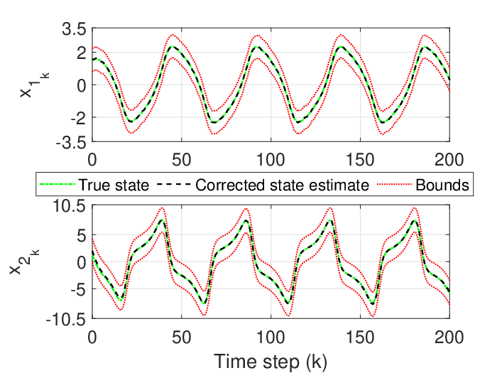
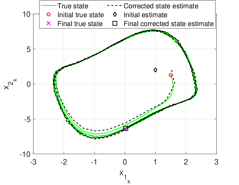
In this example, the initial condition is given by 𝑷0=𝑰2\bm{P}_{0}=\bm{I}_{2}, 𝒙0=[1.51.25]T\bm{x}_{0}=[1.5\quad 1.25]^{\text{T}}, and 𝒙^0=[12]T\hat{\bm{x}}_{0}=[1\quad 2]^{\text{T}}. For Assumption 3.1, we can consider 𝔻0=ℰ⁡(𝒙^0,𝑷0)\mathbb{D}_{0}=\mathcal{E}(\hat{\bm{x}}_{0},\bm{P}_{0}). In terms of Assumption 3.2, let us choose q=r=0.01q=r=0.01. Then, Assumption 3.2 is satisfied with (i) wkw_{k} and vkv_{k} randomly varying (uniform distribution) between -0.05 and 0.05; (ii) 𝑸k=0.01​𝑰2\bm{Q}_{k}=0.01\bm{I}_{2}, 𝑹k=0.01\bm{R}_{k}=0.01. The true state components along with the corresponding corrected state estimates and bounds are shown in Fig. 1 as functions of time steps. Clearly, x1kx_{1_{k}}, x2kx_{2_{k}} remain within the bounds for the entire time-horizon considered which mean that the true state is successfully contained in the correction ellipsoids. Fig. 2 depicts the true state trajectory and the corrected state estimate trajectory in the phase plane. Note that, at k=0k=0, the correction step brings the corrected state estimate close to the initial true state. Also, it is obvious that the corrected state estimate trajectory converges to and remains in a neighborhood of the true state trajectory after a few recursions of the filter.

TABLE I: Mean trace and estimation error comparisons over 200 time steps
Item SDC-SMF Wang et al. [13]
Mean trace 5.5007 6.2616
MAE 0.1142 0.1761
MSE 0.0277 0.0643
Refer to caption
Fig. 3: Estimation error norms for the SDC-SMF and the SMF in [13] (Wang et al.).
Refer to caption
Fig. 4: Trace of correction ellipsoid shape matrices for the SDC-SMF and state estimation ellipsoid shape matrices for the SMF in [13] (Wang et al.).

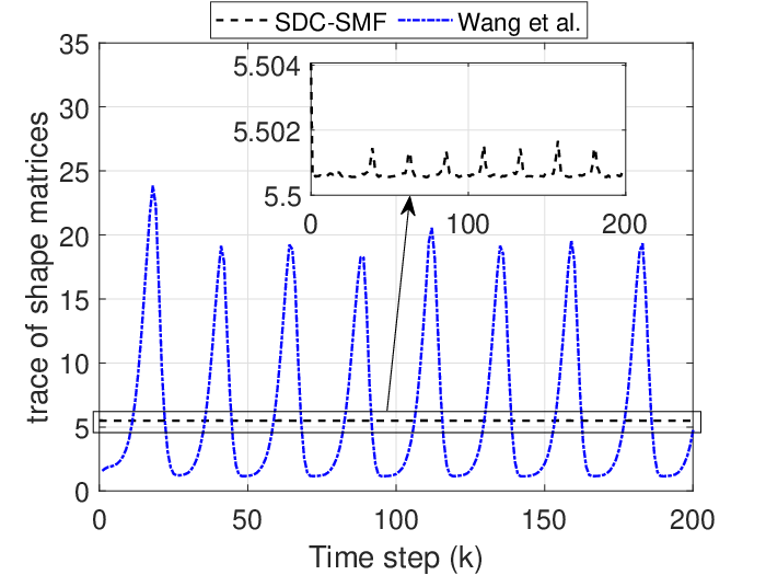
Next, for comparison, we implement the SMF in [13] for the above example with the remainder bounding ellipsoids synthesized using 50 constraints. Let us consider the estimation errors at the correction steps for the SDC-SMF and at the measurement update steps for the SMF in [13]. The comparison in these estimation error norms is shown in Fig. 3 where ‖𝒆0‖=‖𝒙0−𝒙^0‖||\bm{e}_{0}||=||\bm{x}_{0}-\hat{\bm{x}}_{0}|| is the initial error norm and the comparison in trace of the corresponding ellipsoid shape matrices is shown in Fig. 4. The results in Figs. 3, 4 demonstrate that the SDC-SMF outperforms the SMF in [13]. This is further illustrated in the results given in Table I where MAE and MSE stand for mean absolute error and mean squared error, respectively. The SDC-SMF performs much better in terms of these two metrics, as shown in Table I. Also, the mean trace value for the SDC-SMF correction ellipsoid shape matrices is smaller compared to that of the state estimation ellipsoid shape matrices for the SMF in [13]. In summary, the SDC-SMF results in lower estimation errors with lower error bounds for this example.
Refer to caption
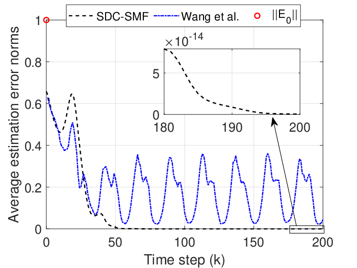
Fig. 5: Average estimation error norms with wk=vk=0w_{k}=v_{k}=0 and nr=10n_{r}=10.

Finally, to demonstrate that the SDC-SMF is asymptotically convergent if there are no process and measurement noises (cf., Section IV), we implement the SDC-SMF for the above example with the initial state randomly chosen from the boundary of the initial ellipsoid ℰ⁡(𝒙^0,𝑷0)\mathcal{E}(\hat{\bm{x}}_{0},\bm{P}_{0}) and with wk=vk=0w_{k}=v_{k}=0. We repeat this process nrn_{r} times. The same is done for the SMF in [13] as well. The average estimation error norms of these runs with the random initializations are shown in Fig. 5 where 𝑬0\bm{E}_{0} is the Cholesky factorization of 𝑷0\bm{P}_{0}. Note that the upper bound of the initial error norm for the random initializations is ‖𝑬0‖||\bm{E}_{0}||, which is shown in Fig. 5. The results in Fig. 5 show that the SDC-SMF is asymptotically convergent with the estimation error tending to zero. However, the SMF in [13] does not exhibit this property, as shown in Fig. 5.

VI Conclusion

A recursive set-membership filtering algorithm for discrete-time nonlinear dynamical systems subject to unknown but bounded process and measurement noise has been derived utilizing the state dependent coefficient (SDC) parameterization. At each time step, the filtering problem has been transformed into two semi-definite programs (SDPs) using the S-procedure and Schur complement. Optimal (minimum trace) ellipsoids have been constructed that contain the true state of the system at the correction and prediction steps. Finally, a simulation example is provided which demonstrates that the proposed filter performs better compared to an existing set-membership filter for discrete-time nonlinear systems. Our future research would involve assessing theoretical properties of the SDC-SMF for systems with control inputs acting through a possibly non-square state-dependent matrix.

Acknowledgment

This research was supported by the Office of Naval Research under Grant No. N00014-18-1-2215. The authors would like to thank the anonymous reviewers for their suggestions which lead to improved quality and presentation of the technical note.

References

  • [1] B. D. Anderson and J. B. Moore, Optimal filtering. Prentice Hall, Inc., 1979.
  • [2] B. T. Polyak, S. A. Nazin, C. Durieu, and E. Walter, “Ellipsoidal parameter or state estimation under model uncertainty,” Automatica, vol. 40, no. 7, pp. 1171–1179, 2004.
  • [3] Y. Becis-Aubry, M. Boutayeb, and M. Darouach, “State estimation in the presence of bounded disturbances,” Automatica, vol. 44, no. 7, pp. 1867–1873, 2008.
  • [4] D. Maksarov and J. Norton, “State bounding with ellipsoidal set description of the uncertainty,” International Journal of Control, vol. 65, no. 5, pp. 847–866, 1996.
  • [5] L. El Ghaoui and G. Calafiore, “Robust filtering for discrete-time systems with bounded noise and parametric uncertainty,” IEEE Transactions on Automatic Control, vol. 46, no. 7, pp. 1084–1089, 2001.
  • [6] F. Yang and Y. Li, “Set-membership filtering for discrete-time systems with nonlinear equality constraints,” IEEE Transactions on Automatic Control, vol. 54, no. 10, pp. 2480–2486, 2009.
  • [7] J. S. Shamma and K.-Y. Tu, “Approximate set-valued observers for nonlinear systems,” IEEE Transactions on Automatic Control, vol. 42, no. 5, pp. 648–658, 1997.
  • [8] G. Calafiore, “Reliable localization using set-valued nonlinear filters,” IEEE Transactions on systems, man, and cybernetics-part A: systems and humans, vol. 35, no. 2, pp. 189–197, 2005.
  • [9] H. Witsenhausen, “Sets of possible states of linear systems given perturbed observations,” IEEE Transactions on Automatic Control, vol. 13, no. 5, pp. 556–558, 1968.
  • [10] F. Schweppe, “Recursive state estimation: unknown but bounded errors and system inputs,” IEEE Transactions on Automatic Control, vol. 13, no. 1, pp. 22–28, 1968.
  • [11] D. Bertsekas and I. Rhodes, “Recursive state estimation for a set-membership description of uncertainty,” IEEE Transactions on Automatic Control, vol. 16, no. 2, pp. 117–128, 1971.
  • [12] G. Wei, S. Liu, Y. Song, and Y. Liu, “Probability-guaranteed set-membership filtering for systems with incomplete measurements,” Automatica, vol. 60, pp. 12–16, 2015.
  • [13] Z. Wang, X. Shen, Y. Zhu, and J. Pan, “A tighter set-membership filter for some nonlinear dynamic systems,” IEEE Access, vol. 6, pp. 25 351–25 362, 2018.
  • [14] Z. Wang, X. Shen, and Y. Zhu, “Ellipsoidal fusion estimation for multisensor dynamic systems with bounded noises,” IEEE Transactions on Automatic Control, vol. 64, no. 11, pp. 4725–4732, 2019.
  • [15] E. Scholte and M. E. Campbell, “A nonlinear set-membership filter for on-line applications,” International Journal of Robust and Nonlinear Control, vol. 13, no. 15, pp. 1337–1358, 2003.
  • [16] B. Zhou, J. Han, and G. Liu, “A ud factorization-based nonlinear adaptive set-membership filter for ellipsoidal estimation,” International Journal of Robust and Nonlinear Control, vol. 18, no. 16, pp. 1513–1531, 2008.
  • [17] C. P. Mracek and J. R. Cloutier, “Control designs for the nonlinear benchmark problem via the state-dependent riccati equation method,” International Journal of robust and nonlinear control, vol. 8, no. 4-5, pp. 401–433, 1998.
  • [18] T. Cimen, “Survey of state-dependent riccati equation in nonlinear optimal feedback control synthesis,” Journal of Guidance, Control, and Dynamics, vol. 35, no. 4, pp. 1025–1047, 2012.
  • [19] A. P. Dani, S.-J. Chung, and S. Hutchinson, “Observer design for stochastic nonlinear systems via contraction-based incremental stability,” IEEE Transactions on Automatic Control, vol. 60, no. 3, pp. 700–714, 2014.
  • [20] C. Jaganath, A. Ridley, and D. S. Bernstein, “A sdre-based asymptotic observer for nonlinear discrete-time systems,” in Proceedings of the American Control Conference, 2005, pp. 3630–3635.
  • [21] I. Chang and J. Bentsman, “High-fidelity discrete-time state-dependent riccati equation filters for stochastic nonlinear systems with gaussian/non-gaussian noises,” in Proceedings of the American Control Conference, 2018, pp. 1132–1137.
  • [22] W. J. Vetter, “Matrix calculus operations and taylor expansions,” SIAM Review, vol. 15, no. 2, pp. 352–369, 1973.
  • [23] M. Vidyasagar, “Nonlinear systems analysis.” SIAM, 2002, ch. 2, pp. 51–52.
  • [24] Y. Song and J. W. Grizzle, “The extended kalman filter as a local asymptotic observer for nonlinear discrete-time systems,” Journal of Mathematical Systems Estimation and Control, vol. 5, no. 1, pp. 59–78, 1995.
  • [25] D. P. Bertsekas, “Convexification procedures and decomposition methods for nonconvex optimization problems,” Journal of Optimization Theory and Applications, vol. 29, no. 2, pp. 169–197, 1979.
  • [26] R. Tempo, G. Calafiore, and F. Dabbene, Randomized algorithms for analysis and control of uncertain systems: with applications. Springer Science & Business Media, 2005.
  • [27] S. H. Brooks, “A discussion of random methods for seeking maxima,” Operations research, vol. 6, no. 2, pp. 244–251, 1958.
  • [28] S. Boyd, L. El Ghaoui, E. Feron, and V. Balakrishnan, Linear matrix inequalities in system and control theory. Siam, 1994, vol. 15.
  • [29] L. Vandenberghe and S. Boyd, “Semidefinite programming,” SIAM review, vol. 38, no. 1, pp. 49–95, 1996.
  • [30] J. Löfberg, “Yalmip: A toolbox for modeling and optimization in matlab,” in Proceedings of the CACSD Conference, vol. 3. Taipei, Taiwan, 2004.