Sideways: Depth-Parallel Training of Video Models

We consider the following general setting:

• •

  a finite input time-series $\bm{x}=(\bm{x}^{t})_{t=1}^{K},\bm{x}^{t}\in\mathbb{R}^{d}$, e.g., a video clip with $d=\text{height}\times\text{width}\times 3$,

• •

  a finite output time-series $\bm{y}=(\bm{y}^{t})_{t=1}^{K},\bm{y}^{t}\in\mathbb{R}^{d_{y}}$, e.g., an action label; in the action recognition task, in our work, we use the same label over the whole video clip, i.e., $\bm{y}^{t}=\bm{y}^{t+1}$ for all $t$,

• •

  a frame-based neural network $\mathcal{M}_{\theta}:\mathbb{R}^{d}\rightarrow\mathbb{R}^{d_{y}}$ that transforms the input signal $\bm{x}^{t}$ into logits $\bm{h}_{D}^{t}=\mathcal{M}_{\theta}(\bm{x}^{t})$, and is defined by a composition of modules

  $$\mathcal{M}_{\theta}(\bm{x}^{t})=H_{D}(\cdot,\theta_{D})\circ H_{D-1}(\cdot,\theta_{D-1})\circ\ldots\circ H_{1}(\bm{x}^{t},\theta_{1})$$

  where:

  • –

    each module, or layer, $H_{i}(\cdot,\cdot)$ is a function $H_{i}:\mathbb{R}^{d_{i-1}}\times\mathbb{R}^{p_{i}}\rightarrow\mathbb{R}^{d_{i}}$, $i=1,\ldots D$,

  • –

    $\theta_{i}\in\mathbb{R}^{p_{i}}$, $i=1,\ldots,D$ are the (trainable) parameters, and we use $\theta$ for all the parameters,

  • –

    $\circ$ is a composition, i.e., $G\circ F(\bm{x})=G(F(\bm{x}))$

  and

• •

  a loss function $\mathcal{L}:\mathbb{R}^{d_{y}}\times\mathbb{R}^{d_{y}}\rightarrow\mathbb{R}$, e.g., $\mathcal{L}(\bm{h},\bm{y})=||\bm{h}-\bm{y}||^{2}$, or $\mathcal{L}(\bm{h},\bm{y})=-\sum_{i}p((\bm{h})_{i})\log q(\bm{y}_{i})$.

We extend the notation above to $\bm{h}_{i}^{t}=H_{i}(\cdot,\theta_{i})\circ H_{i-1}(\cdot,\theta_{i-1})\circ\ldots\circ H_{1}(\bm{x}^{t},\theta_{1})$.

To avoid the common confusion coming from using the same letters to denote both the function formal arguments and actual values of the variables, we will use bold font for the latter, e.g., $x$ to denote a formal argument and $\bm{x}$ for its actual value. We also use the following notation for the derivatives of the functions $H_{i}$. Let $\mathcal{J}_{h}H(\bm{h},\bm{\theta})=\left.\frac{\partial H(h,\bm{\theta})}{\partial h}\right|_{h=\bm{h}}$ be the Jacobian matrix of $H(h,\theta)$ with respect to the variable $h$ evaluated at $h=\bm{h}$, $\theta=\bm{\theta}$. Similarly, $\mathcal{J}_{\theta}H(\bm{h},\bm{\theta})=\left.\frac{\partial H(\bm{h},\theta)}{\partial\theta}\right|_{\theta=\bm{\theta}}$ denote the Jacobian matrix of $H(h,\theta)$ with respect to the variable $\theta$ evaluated at $h=\bm{h}$, $\theta=\bm{\theta}$. We will use the same notation for the gradient $\nabla$.

Finally, to train neural networks, we base our computations on the empirical risk minimization framework, i.e.  $\mathcal{R}(\mathcal{M}_{\theta})=E_{x,y}[\mathcal{L}(\mathcal{M}_{\theta}(x),y)]\approx\sum_{\bm{x},\bm{y}\sim\mathcal{D}}\frac{1}{K}\sum_{t=1}^{K}\mathcal{L}(\bm{h}_{D}^{t},\bm{y}^{t})$, where $\mathcal{D}$ is a training set.

For simplicity, we assume in our modelling a constant time for a layer (or some set of layers organized into a module) to fully process its inputs, both in the forward or backward pass and call this a computation step. We define the update cycle as the sequence of computation steps that a given data frame is used to update all the layers, and the cycle length as the number of computation steps in the update cycle. Hence, the cycle length depends only on the depth of the network $D$ and is equal to $2D-1$ computation steps. Figure 2 illustrates a single update cycle with nine computation steps for both models.

The BP algorithm refers to regular training of neural networks. Here, due to the synchronization between the passes, computations are blocked each time a data frame is processed. This is illustrated in Figure 2 (left). Whenever the first frame is processed, here indicated by the blue square, the computations are blocked in both forward and backward passes over the whole update cycle.

With our notation, the standard backpropagation formula becomes

with the update rule $\theta_{i}:=\theta_{i}-\alpha\frac{1}{K}\sum_{t=1}^{K}\nabla_{\theta_{i}}^{t}\mathcal{L}$, where $\alpha$ is the learning rate, and $K$ is the length of the input sequence.

We can compactly describe the algorithm above with the following recursive rules

where $\bm{h}^{t}_{0}=\bm{x}^{t}$. However, we do not compute Jacobian matrices explicitly; instead efficient vector matrix multiplications are used to backpropagate errors from the loss layer towards the input [1].

We aim at pipelining computations for the whole update cycle during training and inference. Sideways removes synchronization by continuously processing information, either in the forward or backward pass. This is illustrated in Figure 2 (right). Once a data frame is available, it is immediately processed and sent to the next layer, ‘freeing’ the current layer so it can process the next data frame. Hence, in the first computation step of the update cycle, a data frame $\bm{x}^{t}$ is processed by the first Sideways module, freeing resources and ‘sending’ $\bm{h}^{t}_{1}$ to the second Sideways module at computation step $t+1$. At computation step $t+1$, the first module can now take the next data frame $\bm{x}^{t+1}$ for processing, and, simultaneously, the second module processes $\bm{h}_{1}^{t}$; this step results in two representations $\bm{h}_{2}^{t}$ and $\bm{h}_{1}^{t+1}$. Please note that our notation $\bm{h}_{2}^{t}$ does not indicate the current computation step but instead that the representation has originated at $\bm{x}^{t}$. We continue the same process further during the training. This is illustrated in Figure 2, where we use color-encoding to track where the information being processed has originated from. Dotted arrows represents the forward pass.

For simplicity, we assume that the computation of the loss takes no time and does not require an extra computation cycle. In such setting the activation arriving at the loss function computing module at timestep $t$ is $\bm{h}_{D}^{t-D+1}$, an activation spawned by the frame $\bm{x}^{t-D+1}$. Once this final representation $\bm{h}_{D}^{t-D+1}$ is computed at computation step $t$, we calculate its ‘correct’ gradient $\nabla_{h_{D}}^{t}\mathcal{L}(\bm{h}_{D}^{t-D+1},\bm{y}^{t})$, and we backpropagate this information down towards the lower layers of the neural network. This computational process is illustrated in Figure 2 (right) by the solid arrows.

Let us formalize this algorithm in a similar manner to the ‘regular’ backpropagation. In the Sideways algorithm the gradient $\nabla_{\theta_{i}}\mathcal{L}|_{(\bm{x}^{t},\bm{\theta}_{i})}$ is replaced with a pseudo-gradient $\widetilde{\nabla}_{\theta_{i}}\mathcal{L}|_{(\bm{x}^{t},\bm{\theta}_{i})}$, defined as follows

where $t_{i}=t+i-D$.

The equations above can next be written succinctly and recursively as the Sideways backpropagation rules

where $\widetilde{\nabla}^{t-1}_{h_{D}}\mathcal{L}=\nabla_{h_{D}}\mathcal{L}(\bm{h}_{D}^{t-D+1},\bm{y}^{t})$, and $\bm{h}^{t}_{0}=\bm{x}^{t}$.

In the equations above, we use a color-encoding similar to Figure 2 (right) to indicate that we combine information originated from different time steps. For instance, information originated in ‘blue’ and ‘yellow’ input frames is combined (6-th computation step and second-last unit) as indicated by the red circle in Figure 2 (right)). By following the arrows we can track the origins of the combined information.

Due to the nature of these computations, we do not compute proper gradients as the BP algorithm does, but instead we compute their more noisy versions, $\widetilde{\nabla}_{\bm{h}_{i}}\mathcal{L}=\nabla_{\bm{h}_{i}}\mathcal{L}+\epsilon_{i}(\bm{x})$, which we call pseudo-gradients. The amount of noise varies with respect to the smoothness of the input $\bm{x}$, and the number of the layer $i$. That is, deeper layers have less noisy pseudo-gradients, and e.g., the pseudo-gradient of the final layer is exact.

We organize training as a sequence of episodes. Each episode consists of one or more update cycles, runs over the whole sampled video clip $\bm{x}$ or its subsequence, and ends with the weights update. We assume the input $\bm{x}$ is smooth within the episode, e.g., $\bm{x}$ is a video of an action being performed with a reasonable frame-rate. We ‘restart’ Sideways by setting up all the activations and pseudo-gradients to zero whenever we sample a new video to avoid aliasing with a pseudo-gradient originated from a data frame from another video clip, and thus breaking our assumptions about the smoothness of the input sequence. Mini-batching can optionally be applied in the usual way.

We average gradients computed at each layer over all computation steps within the episode, i.e.,

where $L$ is the length of the episode. In our experiments we consider two cases. In the classification task, the episode is the same as the sampled sequence, i.e., $L=K$. In the auto-encoding task, the episode is a single data frame, i.e., $L=1$. We use pseudo-gradients $\widetilde{\nabla}_{\theta_{i}}\mathcal{L}$ for the weight updates, i.e., $\theta_{i}:=\theta_{i}-\alpha\widetilde{\nabla}_{\theta_{i}}\mathcal{L}$.

Figure 3(right) illustrates the situation when the pipeline is full and suggests, the information flow is tilted sideways. Therefore, there is no information available in the upper layers at the beginning of the sequence (empty circles in the figure). For that reason, we modify Equation 5 by including a binary mask, i.e., $\widetilde{\nabla}_{\theta_{i}}\mathcal{L}=\frac{1}{\gamma_{i}}\sum_{t=1}^{L}\gamma_{i}^{t}\widetilde{\nabla}_{\theta_{i}}^{t}\mathcal{L}$, where $\gamma_{i}=\sum_{t}\gamma_{i}^{t}$. The mask is zero for unavailable gradients. For similar reasons, to avoid gradient computations whenever suitable information is unavailable, we modify Equation 4 with $\widetilde{\nabla}_{\bm{h}_{i}}^{t}\mathcal{L}=\gamma_{i}^{t}\widetilde{\nabla}_{h_{i}}^{t-1}\mathcal{L}\cdot\mathcal{J}_{h_{i-1}}H_{i}(\bm{h}_{i-1}^{t-i+1},\bm{\theta}_{i})$. Without masking, we have observed more unstable training in practice.

We benchmark our algorithms on two different tasks and three datasets.

We choose to benchmark our models of computations on the following video datasets. On one hand, first two datasets have enough complexity and realism. On the other hand, we can easily train frame-based video models on all the following datasets.

UCF101 is another popular dataset for action recognition [48]. It has 13320 videos clips and 101 human actions. Actions include pizza tossing, typing, playing cello, skiing, etc. Default frame-rate is $25$fps, with the duration of $7.21$sec on average. Each frame has resolution $320$-by-$240$. We use train and test splits in our studies. In our experiments, we find this dataset to be of particular interest due to its size, complexity, and realism.

CATER dataset [15] provides synthetically generated videos of moving simple 3D objects. We use only the video frames and we set up an unsupervised auto-encoding task. These videos have two desired properties – i) they are visually simple, and ii) they have diverse motion patterns of various objects – making it an excellent benchmark for Sideways. We use the pre-generated video sequences provided by the authors in the all_actions subset, consisting of 3861 training video sequences and 1639 test sequences, each with 300 frames, having $320$-by-$240$ pixels resolution at $24$fps.

For the purposes of our study we have experimented with two standard convolutional network architectures. The first one is organized into 6 Sideways modules, another one with 8 Sideways modules. Note, however, that we can use more than one trainable layers inside a single Sideways module.

For the auto-encoding experiments, we train a simple encoder-decoder architecture having the same five convolutional blocks followed by symmetrical five deconvolutional blocks. We use Sideways blocks only for the convolutional encoder; the decoder layers are connected all in a single sequential block, and hence the decoder-block is trained with a regular BP with ‘correct’ gradients. For simplicity, we also assume the whole decoder takes just a single computation step. We use this setting to better investigate the quality of the features extracted by the Sideways encoder.

VGG-net refers to VGG-8, which is a direct re-implementation of the RGB network in the original two-stream model [47] with the addition of batchnorm in every VGG-block (in between the convolution and the ReLU).

In some experiments we use batchnorm [23] and dropout [49] in linear layers ($0.9$ as [46]). In most training experiments, we use a single GPU (V100) – but measure parallelization speedup later in the section using multiple GPUs. We decouple the weight decay term from the loss [33] and find that some amount of weight decay is beneficial for generalization of the VGG-net models. We do a hyper-parameter search over the weight decay coefficient (possible values are: $0.0,10^{-4},10^{-3},10^{-2}$), and over the initial learning rate (either $10^{-4}$ or $10^{-5}$), fairly for both types of training.

We train on videos with the per-frame resolution $112$-by-$112$ and a sequence length $64$ randomly cropped from the whole video clip as a contiguous subsequence. We also use random flipping during training, and this augmentation is performed consistently over all the frames in every clip. At test time we simply take a center crop of a video frame. In all cases, we use torus-padding (video frames are repeated) whenever a sampled video clip is shorter than $64$ and at test time we evaluate over the whole video sequence. In practice we use a fixed batch size of 8 videos for training.

For the auto-encoding experiments with CATER, we use square crops of 240$\times$240 pixels, extracted randomly during training and central crops of the same size during testing.

We have evaluated networks trained with Sideways and BP according to the regular accuracy metric. Moreover, to gain a better understanding, and to show how general the Sideways training is, we have conducted several different experiments measuring not only accuracy but also training dynamics and robustness of the method.

Results presented in Table 1 suggest that the Sideways training achieves competitive accuracy to BP, and the introduced noise due to i) the sampling error, the same as SGD updates, and ii) the pseudo-gradients computations, does not seem to harm the overall performance. Quite the opposite, under certain conditions, we observe Sideways generalizes better than BP. Since such behavior occurs during training larger models on relatively small video datasets, e.g., training VGG-8 on UCF-101, which often results in overfitting [46], we hypothesize Sideways acts as an implicit regularizer for video processing [38, 55].

We evaluate both algorithms using mean squared error, between pixels, between the predicted and the ground truth sequences, under the same conditions, in particular, under the same frame rate.

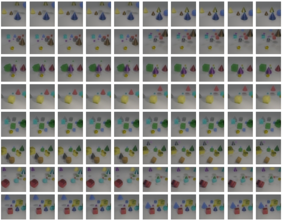
Qualitative results. We show qualitative results of the BP outputs in Figure 7 and Sideways outputs in Figure 8. Shapes, colors, as well as many fine-grained attributes such as metallic materials are properly decoded. We have found that the model trained with BP is successful at decoding coarser objects attributes, but is slightly less accurate with metallic materials. As mentioned above, because of the blocking mechanism of the BP algorithm and the high frame rate of the input, the method needs to discard input frames to not accumulate latency. In these cases, the last produced output is copied to compensate for the low output rate, resulting in identical output frames at different time steps over some time interval – and different ones at the beginning of the next update cycle (this is best visible in the 1st row of Figure 7).

Quantitative results. Table 3 shows mean squared error (the lower, the better) between predicted frames and ground truth (input frames). We compare the same architecture trained with Sideways and the regular BP. Because of the synchronization, the method trained with BP cannot output at a fast enough pace to keep up with the input frame rate, which yields a significant error.

These results show that the proposed training scheme can be successfully applied also to tasks where both input and output are continuously evolving, reducing considerably the latency of the system during training. Together with the results on the classification task, we conclude that this training scheme is general enough to be applied for a wide range of video tasks.

References

- Abadi et al. [2016] M. Abadi, A. Agarwal, P. Barham, E. Brevdo, Z. Chen, C. Citro, G. S. Corrado, A. Davis, J. Dean, M. Devin, et al. Tensorflow: Large-scale machine learning on heterogeneous distributed systems. arXiv preprint arXiv:1603.04467, 2016.
- Balduzzi et al. [2015] D. Balduzzi, H. Vanchinathan, and J. Buhmann. Kickback cuts backprop’s red-tape: Biologically plausible credit assignment in neural networks. In AAAI Conference on Artificial Intelligence, 2015.
- Belilovsky et al. [2019] E. Belilovsky, M. Eickenberg, and E. Oyallon. Decoupled greedy learning of cnns. arXiv preprint arXiv:1901.08164, 2019.
- Bengio et al. [2015a] E. Bengio, P.-L. Bacon, J. Pineau, and D. Precup. Conditional computation in neural networks for faster models. In 2nd Multidisciplinary Conference on Reinforcement Learning and Decision Making (RLDM), 2015a.
- Bengio et al. [2015b] Y. Bengio, D.-H. Lee, J. Bornschein, T. Mesnard, and Z. Lin. Towards biologically plausible deep learning. arXiv preprint arXiv:1502.04156, 2015b.
- Betti and Gori [2019] A. Betti and M. Gori. Backprop diffusion is biologically plausible. arXiv preprint arXiv:1912.04635, 2019.
- Bottou and Cun [2004] L. Bottou and Y. L. Cun. Large scale online learning. In Advances in Neural Information Processing Systems (NeurIPS), 2004.
- Carreira and Zisserman [2017] J. Carreira and A. Zisserman. Quo vadis, action recognition? a new model and the kinetics dataset. In Conference on Computer Vision and Pattern Recognition (CVPR), 2017.
- Carreira et al. [2018] J. Carreira, V. Patraucean, L. Mazare, A. Zisserman, and S. Osindero. Massively parallel video networks. In European Conference on Computer Vision (ECCV), 2018.
- Choromanska et al. [2015] A. Choromanska, M. Henaff, M. Mathieu, G. B. Arous, and Y. LeCun. The loss surfaces of multilayer networks. In Artificial Intelligence and Statistics, 2015.
- Choromanska et al. [2019] A. Choromanska, B. Cowen, S. Kumaravel, R. Luss, M. Rigotti, I. Rish, B. Kingsbury, P. DiAchille, V. Gurev, R. Tejwani, et al. Beyond backprop: Online alternating minimization with auxiliary variables. In International Conference on Machine Learning (ICML), 2019.
- Czarnecki et al. [2017] W. Czarnecki, G. Świrszcz, M. Jaderberg, S. Osindero, O. Vinyals, and K. Kavukcuoglu. Understanding synthetic gradients and decoupled neural interfaces. In International Conference on Machine Learning (ICML), 2017.
- Diba et al. [2019] A. Diba, V. Sharma, L. Van Gool, and R. Stiefelhagen. Dynamonet: Dynamic action and motion network. In IEEE International Conference on Computer Vision (ICCV), 2019.
- Duchi et al. [2011] J. Duchi, E. Hazan, and Y. Singer. Adaptive subgradient methods for online learning and stochastic optimization. Journal of Machine Learning Research (JMLR), 2011. ISSN 1532-4435.
- Girdhar and Ramanan [2020] R. Girdhar and D. Ramanan. Cater: A diagnostic dataset for compositional actions and temporal reasoning. International Conference on Learning Representations (ICLR), 2020.
- Goyal et al. [2017] P. Goyal, P. Dollár, R. Girshick, P. Noordhuis, L. Wesolowski, A. Kyrola, A. Tulloch, Y. Jia, and K. He. Accurate, large minibatch sgd: Training imagenet in 1 hour. arXiv preprint arXiv:1706.02677, 2017.
- Hara et al. [2018] K. Hara, H. Kataoka, and Y. Satoh. Can spatiotemporal 3d cnns retrace the history of 2d cnns and imagenet? In Computer Vision and Pattern Recognition (CVPR), 2018.
- He et al. [2019] K. He, R. Girshick, and P. Dollár. Rethinking imagenet pre-training. In International Conference on Computer Vision (ICCV), 2019.
- Hinton [1990] G. E. Hinton. Connectionist learning procedures. In Machine learning, pages 555–610. Elsevier, 1990.
- Huang et al. [2018] Y. Huang, Y. Cheng, D. Chen, H. Lee, J. Ngiam, Q. V. Le, and Z. Chen. Gpipe: Efficient training of giant neural networks using pipeline parallelism. In Advances in Neural Information Processing Systems (NeurIPS), 2018.
- Huo et al. [2018a] Z. Huo, B. Gu, and H. Huang. Training neural networks using features replay. In Advances in Neural Information Processing Systems, pages 6659–6668, 2018a.
- Huo et al. [2018b] Z. Huo, B. Gu, Q. Yang, and H. Huang. Decoupled parallel backpropagation with convergence guarantee. In International Conference on Machine Learning (ICML), volume 80, 2018b.
- Ioffe and Szegedy [2015] S. Ioffe and C. Szegedy. Batch normalization: Accelerating deep network training by reducing internal covariate shift. In International Conference on Machine Learning (ICML), 2015.
- Jaderberg et al. [2017] M. Jaderberg, W. M. Czarnecki, S. Osindero, O. Vinyals, A. Graves, D. Silver, and K. Kavukcuoglu. Decoupled neural interfaces using synthetic gradients. In International Conference on Machine Learning (ICML), 2017.
- Jing and Tian [2018] L. Jing and Y. Tian. Self-supervised spatiotemporal feature learning by video geometric transformations. arXiv preprint arXiv:1811.11387, 2018.
- Karpathy et al. [2014] A. Karpathy, G. Toderici, S. Shetty, T. Leung, R. Sukthankar, and L. Fei-Fei. Large-scale video classification with convolutional neural networks. In Computer Vision and Pattern Recognition (CVPR), 2014.
- Kingma and Ba [2014] D. Kingma and J. Ba. Adam: A method for stochastic optimization. International Conference on Learning Representations (ICLR), 12 2014.
- Korbar et al. [2019] B. Korbar, D. Tran, and L. Torresani. Scsampler: Sampling salient clips from video for efficient action recognition. In 2011 International Conference on Computer Vision (ICCV), 2019.
- Kubilius et al. [2018] J. Kubilius, M. Schrimpf, A. Nayebi, D. Bear, D. L. Yamins, and J. J. DiCarlo. Cornet: modeling the neural mechanisms of core object recognition. BioRxiv, 2018.
- Kuehne et al. [2011] H. Kuehne, H. Jhuang, E. Garrote, T. Poggio, and T. Serre. Hmdb: a large video database for human motion recognition. In 2011 International Conference on Computer Vision (ICCV), 2011.
- Larkum [2013] M. Larkum. A cellular mechanism for cortical associations: an organizing principle for the cerebral cortex. Trends in neurosciences, 36(3):141–151, 2013.
- Lillicrap et al. [2016] T. P. Lillicrap, D. Cownden, D. B. Tweed, and C. J. Akerman. Random synaptic feedback weights support error backpropagation for deep learning. Nature Communications, 2016.
- Loshchilov and Hutter [2019] I. Loshchilov and F. Hutter. Decoupled weight decay regularization. In International Conference on Learning Representations (ICLR), 2019.
- Löwe et al. [2019] S. Löwe, P. O’Connor, and B. Veeling. Putting an end to end-to-end: Gradient-isolated learning of representations. In Advances in Neural Information Processing Systems (NeurIPS), 2019.
- Malinowski et al. [2018] M. Malinowski, C. Doersch, A. Santoro, and P. Battaglia. Learning visual question answering by bootstrapping hard attention. In European Conference on Computer Vision (ECCV), 2018.
- Metz et al. [2019] L. Metz, N. Maheswaranathan, B. Cheung, and J. Sohl-Dickstein. Learning unsupervised learning rules. In International Conference on Learning Representations (ICLR), 2019.
- Mnih et al. [2014] V. Mnih, N. Heess, A. Graves, et al. Recurrent models of visual attention. In Advances in Neural Information Processing Systems (NeurIPS), 2014.
- Neyshabur [2017] B. Neyshabur. Implicit regularization in deep learning. arXiv preprint arXiv:1709.01953, 2017.
- Nøkland [2016] A. Nøkland. Direct feedback alignment provides learning in deep neural networks. In Advances in Neural Information Processing Systems (NeurIPS), 2016.
- Nøkland and Eidnes [2019] A. Nøkland and L. H. Eidnes. Training neural networks with local error signals. arXiv preprint arXiv:1901.06656, 2019.
- Oord et al. [2018] A. v. d. Oord, Y. Li, and O. Vinyals. Representation learning with contrastive predictive coding. arXiv preprint arXiv:1807.03748, 2018.
- Real et al. [2019] E. Real, A. Aggarwal, Y. Huang, and Q. V. Le. Regularized evolution for image classifier architecture search. In AAAI Conference on Artificial Intelligence (AAAI), 2019.
- Recht et al. [2011] B. Recht, C. Re, S. Wright, and F. Niu. Hogwild: A lock-free approach to parallelizing stochastic gradient descent. In Advances in neural information processing systems, 2011.
- Robbins and Monro [1951] H. Robbins and S. Monro. A stochastic approximation method. The annals of mathematical statistics, 1951.
- Shen et al. [2019] Z. Shen, Z. Liu, J. Li, Y.-G. Jiang, Y. Chen, and X. Xue. Object detection from scratch with deep supervision. IEEE Transactions on Pattern Analysis and Machine Intelligence (TPAMI), 2019.
- Simonyan and Zisserman [2014] K. Simonyan and A. Zisserman. Two-stream convolutional networks for action recognition in videos. In Advances in Neural Information Processing Systems (NeurIPS), 2014.
- Simonyan and Zisserman [2015] K. Simonyan and A. Zisserman. Very deep convolutional networks for large-scale image recognition. International Conference on Learning Representations (ICLR), 2015.
- Soomro et al. [2012] K. Soomro, A. R. Zamir, and M. Shah. Ucf101: A dataset of 101 human actions classes from videos in the wild. arXiv preprint arXiv:1212.0402, 2012.
- Srivastava et al. [2014] N. Srivastava, G. Hinton, A. Krizhevsky, I. Sutskever, and R. Salakhutdinov. Dropout: a simple way to prevent neural networks from overfitting. The journal of machine learning research (JMLR), 15(1):1929–1958, 2014.
- Sutskever et al. [2013] I. Sutskever, J. Martens, G. Dahl, and G. Hinton. On the importance of initialization and momentum in deep learning. In International Conference on International Conference on Machine Learning (ICML), 2013.
- Tomita et al. [1999] H. Tomita, M. Ohbayashi, K. Nakahara, I. Hasegawa, and Y. Miyashita. Top-down signal from prefrontal cortex in executive control of memory retrieval. Nature, 401(6754), 1999.
- Vaswani et al. [2017] A. Vaswani, N. Shazeer, N. Parmar, J. Uszkoreit, L. Jones, A. N. Gomez, Ł. Kaiser, and I. Polosukhin. Attention is all you need. In Advances in Neural Information Processing Systems (NeurIPS), 2017.
- Wiskott and Sejnowski [2002] L. Wiskott and T. J. Sejnowski. Slow feature analysis: Unsupervised learning of invariances. Neural computation, 14(4):715–770, 2002.
- Wu et al. [2019] W. Wu, D. He, X. Tan, S. Chen, and S. Wen. Multi-agent reinforcement learning based frame sampling for effective untrimmed video recognition. CoRR, abs/1907.13369, 2019.
- Zhang et al. [2017] C. Zhang, S. Bengio, M. Hardt, B. Recht, and O. Vinyals. Understanding deep learning requires rethinking generalization. International Conference on Learning Representations (ICLR), 2017.
- Zhang [2004] T. Zhang. Solving large scale linear prediction problems using stochastic gradient descent algorithms. In International Conference on Machine learning (ICML). ACM, 2004.
Acknowledgements
We thank Jean-Baptiste Alayrac, Carl Doersch, Tamara Norman, Simon Osindero, and Andrew Zisserman for their critical feedback, and their help during the duration of this project.