A Derivative-Free Method for Solving Elliptic Partial Differential Equations with Deep Neural NetworksJournal: the arXiv

There is an equivalence between the solutions of quasilinear elliptic PDEs and stochastic processes with the martingale property, which we briefly review here. We are interested in the quasilinear elliptic PDE,

in which $F=F(x,u(x),\nabla u(x),\ldots)\in\mathbb{R}^{d}$ and $G=G(x,u(x),\nabla u(x),\ldots)\in\mathbb{R}$ may depend locally on the unknown function $u$. For ease of notation we will write $F(x,u(x))$, $G(x,u(x))$ and suppress the possible dependence on higher derivatives. Define the stochastic process $X_{t}\in\mathbb{R}^{d}$ as a solution to the stochastic differential equation

in which $B_{t}\in\mathbb{R}^{d}$ is an ordinary Brownian motion on $\mathbb{R}^{d}$, $F$ is the function from the PDE, Eq. (1), and $u:\Omega\to\mathbb{R}$ is arbitrary.

Define the stochastic process $f(t,X_{t})\in\mathbb{R}$ by

for arbitrary $u:\Omega\to\mathbb{R}$. Note that $f(t,X_{t})$ actually depends on the entire history $\{X_{s}\}_{s\leq t}$ but we write it $f(t,X_{t})$ for convenience of notation.

With these definitions, the following two statements are equivalent:

• 1.

  $u:\Omega\to\mathbb{R}$ is a solution to the PDE in Eq. (1): $\mathcal{Q}(u)(x)=0$ for all $x\in\Omega$;

• 2.

  the stochastic process $f(t,X_{t})$ satisfies the martingale property

  $$\mathbf{E}\left[f(t,X_{t})\left|X\right._{0}=x\right]-f(0,x)=0\textrm{~for all~}x\in\Omega,t>0.$$

  (4)

This equivalence is a standard application of Itô’s lemma (see e.g. KS), Moreover, Itô’s lemma shows that the infinitesimal drift of the stochastic process $f(t,X_{t})$ is precisely $\mathcal{Q}(u)$ in the sense that

which holds as $\Delta t\to 0$. This drift is identically zero on $\Omega$ precisely when $u$ satisfies the PDE. Having zero drift everywhere in the domain is equivalent to $f(t,X_{t})$ satisfying the martingale property. Both Eqs. (4) and (5) exchange solving a PDE $\mathcal{Q}(u)=0$ into finding a martingale $f$.

In order to impose a boundary condition, for example of the form

we required that $f(0,x)=h(x)$ for $x\in\partial\Omega$. This follows from Eq. (3), since $f(0,x)=u(x)$ for all $x$. In contrast, homogeneous Neumann conditions of the form

can be imposed by reflecting $X_{t}$ in the normal direction on the boundary $\partial\Omega$. Mixtures between these two boundary conditions, with Dirichlet on part of $\partial\Omega$ and Neumann on another part of $\partial\Omega$, requires a straightforward modification.

In the previous section, we transformed the search for a function $u$ that satisfies the PDE Eq. (1) into a search for the function $f$ that has the martingale property, Eq. (4). As a motivating case, consider the linear elliptic boundary value problem,

Using the equivalence from the previous section, $u$ is the solution of Eq. (8) if and only if the stochastic process $f(t,X_{t})$ is a martingale satisfying $f(0,x)=h(x)$, where $f(t,X_{t})$ is defined as

and $X_{t}$ is the stochastic process which satisfies the stochastic differential equation,

In particular, by using the martingale property for $f$, the solution $u$ satisfies the following relation for any $t>0$ and any $X_{0}\in\Omega$,

Note that Eq. (11) is also true when $t$ is a stopping time by application of the Doob’s optional stopping time theorem (see e.g. KS). By using the stopping time $t=\inf\{s:X_{s}\not\in\Omega\}$, one obtains the well known Feynman-Kac formula for this PDE, the basis of many Monte Carlo algorithms.

Equation (11) also appears in the context of Markov reward processes where it is known as the Bellman equation and the unknown function $u$ is known as the value function. Reinforcement learning SUTTON is a subfield of machine learning that has developed very powerful tools for numerically computing the value function in situations of this form. Algorithms such as temporal difference learning SUTTON or the deep Q-learning method DEEPQ have been developed that apply very generally to this situation. Reinforcement learning techniques are usually applied to the even more complicated Markov decision process, where not only is the value function unknown, but the optimal action is also unknown. Our situation is simpler because there is no unknown action policy to be learned.

In our numerical method, we will consider a class of parametrized functions $u_{\theta}(x)=u(x;\theta)$, and search for parameters $\theta$ such that Eq. (11) holds. We choose to use neural networks as our class of parametrized functions $u_{\theta}$, as will be described in Section 3. Our method is not limited to this choice - any collection of arbitrary function approximators may be used.

Our search method to find the parameters $\theta$ is inspired by techniques from reinforcement learning. We fix a timestep $\Delta t$, and construct an objective function which measures how well Eq. (11) is satisfied as a function of parameters $\theta$,

In Eq. (12), the inner expectation is over the trajectory and the outer expectation is over the initial locations $x$. Essentially, our algorithm performs gradient descent on this function to obtain a sequence of parameters $\theta_{1},\theta_{2},\ldots$ that successively reduces $\mathcal{L}(\theta)$ making $u$ closer to solving Eq. (8). Section 3.2 provides the exact details on how this gradient descent is implemented in our method.

Since $\Delta t$ is small, one can think of the objective function Eq. (12) as approximating the value of the PDE $\mathcal{Q}(u)$ as described in Eq. (5). We emphasize that many other more involved methods from reinforcement learning can be applied to solve the Bellman equation Eq. (11); the simple $L_{2}$ objective function we use here has this added interpretation of directly approximating the PDE.

The stochastic process $X_{t}$ explores the domain and contributes to learning the solution of the PDE at its location. The stochastic processes defined above in Eq. (2) or Eq. (10) might have a nontrivial drift that causes the stochastic process to be driven away from an important area of the domain. It may also have a small volatility that causes slow movement and therefore slow learning or a data imbalance in sampling and therefore an inaccurate solution. Both of these issues are discussed with respect to the example in Section 4.2.

To avoid these issues, we use an alternative martingale process $f(t,X_{t})$ with $X_{t}$ an ordinary Brownian motion, denoted $B_{t}$. Being able to transformation from a possibly complicated process $X_{t}$ to a Brownian motion $B_{t}$ is a result of the Cameron-Martin-Girsanov theorem (see e.g. KS). Applying this theorem, we find that the function $u:\Omega\to\mathbb{R}$ satisfies the PDE Eq. (1) if and only if the stochastic process

is a martingale. In Eq. (13), $B_{t}\in\Omega\subset\mathbb{R}^{d}$ is a Brownian motion on the time interval $t\in[0,\infty)$ starting from an arbitrary initial condition $B_{0}\in\Omega$. In order to remove the drift from the stochastic process $X_{t}$, the martingale process Eq. (13) now contains an additional exponential factor, which can be thought of as discounting rewards obtained when $B_{t}$ happens to move in the upwind direction of the drift in $X_{t}$. Using the Cameron-Martin-Girsanov theorem allows the Brownian walkers to explore the domain unimpeded regardless of the PDE being solved.

From the martingale property for $f$ in Eq. (13), the solution $u$ of the Eq. (1) satisfies the following relation for any $0<t$,

We search for the parametrized function $u(x;\theta)$ to minimize the residual in Eq. (14) by minimizing the following objective function

where $f_{\theta}$ is given by as Eq. (13) with the parameterized function $u(x;\theta)$.

Neural networks are widely used in many applications including computer vision BISHOPPATTERN, natural language processing NATURALNEURAL, forecasting, and speech recognition NEURALSPEECH. The structures of neural networks are designed to extract the valuable features from data. For instance, a convolutional neural network (CNN) is suitable for image data while a recurrent neural network (RNN) is well-suited for capturing sequential information from data.

In this work, we consider the multilayer perceptron (MLP) GOODFELLOW and a simple variant of the residual neural network (ResNet) RESNET as the parameterized approximation $u(x;\theta)$ of the solution. Other architectures are compatible with our method but not explored here. In particular, the accuracy of the neural network could be improved by including problem-specific information, but we do not focus on network architecture engineering in this study.

The core of the method is computing and minimizing, with gradient descent, the residual of the Bellman equation for the stochastic process $f(t,B_{t})$ in Eq. (13) (or Eq. (3) if the Cameron-Martin-Girsanov theorem is not being used). The psuedocode for our method is shown in Algorithm 1. Evaluating Eq. (13) with $t=\Delta t$, we see that a function $u$ is a solution if and only if $u$ satisfies

in which $\mathcal{D}$ and $\mathcal{R}$ are discounts and rewards defined as

The goal is to find parameters $\theta$ such that the neural network $u_{\theta}(x):=u(x;\theta)$ satisfies Eq. (19). To achieve this, the training methodology is to create a sequence of parameters $\theta_{1},\theta_{2},\ldots$, where each set of parameters $\theta_{n}$ is determined from $\theta_{n-1}$ by a stochastic gradient descent update of a loss function $\mathcal{L}_{n}(\theta)$. The loss function $\mathcal{L}_{n}$ combines information from the interior of $\Omega$ obtained from a random sample of the expression in Eq. (15) and a contribution from the boundary $\partial\Omega$.

We simulate discrete Brownian motions $B_{t}^{(i)}$, $i=1,\cdots,N$, which run in the interior of $\Omega$ independently and simultaneously. The interior loss function is defined as

The target values are

in which $D(F,u)$ and $R(G,u)$ are the discretizations of $\mathcal{D}(F,u)$ and $\mathcal{R}(G,u)$ respectively, given as

It is important to note that the discretizations $D$ and $R$ above result in a discrete-time stochastic process $u(B_{n\Delta t})D-R$ that has the martingale property like the continuous-time process $u(B_{t})\mathcal{D}-\mathcal{R}$. Also note that the target values in Eq. (23) depend on the previous parameters $\theta_{n-1}$ and not the argument $\theta$ to the loss function.

It is possible that a Brownian walker will exit the domain between time 0 and $\Delta t$. We detect this by $B_{\Delta t}\not\in\Omega$, which is an admittedly biased sampling of the exit since an exit may have occurred when $B_{\Delta t}\in\Omega$. If a Brownian walker exits the domain, we approximate the exit position on the boundary $\partial\Omega$ by the intersection of line segment between $B_{0}$ and $B_{\Delta t}$ and the boundary $\partial\Omega$. We also approximate the exit time by linearly interpolating in time according to the approximated exit position in the line segment between $B_{0}$ and $B_{\Delta t}$. The approximation of the exit position and time is used in calculating the target value in Eq. (23) instead of the value of $u$ from the neural network. This target value is rich in the information of the exact solution since the exact value of function is given from the boundary condition. To enhance the information available on the boundary, we included an additional term in our loss function,

We train the neural network by minimizing the loss function,

by sequentially updating the parameters with stochastic gradient descent,

The learning rate $\alpha$ may be adjusted on each step. In practice, this gradient descent step can be optimized to take previous steps into account, for example by using the ADAM optimization method ADAM.

As a representative example of a problem in elliptic PDEs, we apply our method to solve Laplace’s equation with a Dirichlet boundary condition,

The domain $\Omega\in\mathbb{R}^{2}$ is a circular sector $\Omega=\{(r,\theta):0\leq r\leq 1,~0\leq\theta\leq\frac{\pi}{6}\}$ and $h$ is the given boundary values. We choose this boundary data by evaluating a harmonic function in $\Omega$ on $\partial\Omega$. This provides us with an exact solution to the problem. We use two different harmonic functions $u_{1}(x_{1},x_{2})=x_{1}^{2}-x_{2}^{2}-\frac{1}{4}x_{1}x_{2}$ and $u_{2}(r,\theta)=r^{\frac{2}{3}}\sin\left(\frac{2}{3}\theta\right)$. Note that $u_{1}$ is smooth on $\Omega\cup\partial\Omega$, but the derivatives of $u_{2}$, $\partial_{r}u_{2}$ and $\partial^{2}_{r}u_{2}$, have a singularity at the origin. The elliptic problem with $u_{2}$ as the solution is known as a corner singularity problem CORNERSINGULARITY, which is a benchmark for testing new numerical algorithms.

The Bellman equation corresponding to Eq. (29) is, for any $t_{0}<t$,

Our method is to find $\theta$ that minimizes the residual of Eq. (30).

For these test problems, we compare our method with another method DGM, PINN, raissi2018forward, raissi2018deep that uses a deep neural network that is explicitly differentiated with respect to its input neurons. We refer to this method as the derivative-based loss method (DBLM), which essentially finds $\theta$ that minimizes the residual of

Note that $\partial^{2}_{x_{i}}u(x;\theta)$, $i=1,2$ are derivatives of the neural network which can be computed using automatic differentiation, i.e backpropagation. The parameters $\theta$ are founded by stochastic gradient method using the loss function at each iteration,

where $x_{i}$, $i=1,2,\cdots,N$ are mini-batch samples in $\Omega$ and $z_{k}$, $k=1,2,\cdots,S$ are mini-batch samples on $\partial\Omega$. The DFLM uses the positions of $N$ independent Brownian motions at each discrete time $n\Delta t$ as minibatch samples in $\Omega$. In the DBLM, uniform minibatch sampling on $\Omega$ at each iteration is used since it yields faster training speed than using Brownian walker sampling.

In order to compare the two methods, we use the multilayer perceptron and a variant of ResNet (defined in Section 3.1) with 4 different activation functions, LReLU, ELU, $\tanh$, and SWISH SWISH. All hyperparameters are identical between the two methods. The MLP has the dimension $[2,20,20,20,20,1]$ and the ResNet is constructed as the stacks of 3 identical residual blocks with the dimension $[20,20,20]$. The hyperparameters, $N=1500$ (the number of Brownian walkers in the DFLM and mini-batch samples in $\Omega$ for the DBLM), $S=300$ (the number of mini-batch samples on $\partial\Omega$ for both methods), $M=200$ (the number of samples for the estimation of the targets in the DFLM) and $\Delta t=$5.0e-4 (the discrete timestep of Brownian motion in the DFLM) are chosen, and the ADAM optimization method with an exponentially decaying learning rate is used to train the neural networks. The relative $\mathcal{L}_{2}$-errors of the numerical solutions after $10^{5}$ iterations is presented in Table 1. The table also shows the error when the network is trained directly using samples of the exact solution. More detailed results are presented in Fig. 1.

The ResNet is more effective than MLP for both methods, and when using the DFLM, the ResNet with SWISH activation approximates the solutions $u_{1}$ and $u_{2}$ with the highest accuracy. The convergence of the DFLM is relatively insensitive to the choice of activation function as can be seen in Fig. 1 (a) and (b)). Also, in this example, the training of our DFLM converges in less (wall-)time than the DBLM.

Interface problems arise when modeling diverse physical and biological phenomena such as electrostatics in composite materials, multiphase flow in fluid dynamics, heat conduction, and the electrical activity of biological cells. In this section, we solve the elliptic equation governing the electric potential on a domain with a single interface. Our method requires a small modification to account of the interface conditions. Although our example has only a single simple interface, our method is easily applied to problems with multiple, possible intricate, interfaces.

Let $\Omega$ be the bounded domain in $\mathbb{R}^{2}$, which consists of two subdomains $\Omega_{0}=\{(r,\theta):0\leq r<1\}$ and $\Omega_{1}=\{(r,\theta):1<r<2\}$ with the interface $\Gamma=\{(r,\theta):r=1\}$. The conductivity $\sigma$ on each $\Omega_{i}$ has constant value $\sigma_{i}$ for $i=0,1$ and the potential difference $\Delta V$ is given across the interface $\Gamma$. The electric potential function $u(x)$ satisfies

The function $g$ in Eq. (33) is the given source distribution over $\Omega$ and the function $h$ in Eq. (34) is the potential on the boundary $\partial\Omega$. Equation (35) is the jump condition resulting from a voltage difference across $\Gamma$. Equation. (36) is the flux continuity condition across the interface $\Gamma$. Here $[q]$ is defined as $[q(x_{0})]=q^{+}(x_{0})-q^{-}(x_{0})$ where $q^{+}(x_{0})$ is the limit of $q(x)$ as $x\rightarrow x_{0}$ from $\Omega_{1}$ and $q^{-}$ is from $\Omega_{0}$.

To appreciate the idea of the modification we make to our method to satisfy the conditions Eq. (35) and Eq. (36), consider the Bellman equation corresponding to Eq. (33) without applying the Cameron-Martin-Girsanov theorem, as discussed in Eq. (10) and (11),

The Brownian walkers take steps from $X_{0}$ and $X_{\Delta t}$ according to

for a time step $\Delta t$. For $X_{0}$ in $\Omega_{0}$ ($\Omega_{1}$) near the interface $\Gamma$, if $X_{\Delta t}$ is in $\Omega_{1}$ ($\Omega_{0}$), the value $u(X_{\Delta t})$ is approximately equal to $u(X_{0})+\Delta V$ ($u(X_{0})-\Delta V$) by the jump condition Eq. (35). Thus, we modify the Bellman equation Eq. (37) to

Next, in order to address the continuity condition Eq. (36), let’s assume $X_{0}$ in $\Omega_{0}$ near the interface $\Gamma$. Since $\sigma$ is constant on $\Omega_{0}$ as $\sigma_{0}$,

in which the distribution of $X_{\Delta t}$ is symmetric with respect to $X_{0}$ and only depends on the conductivity $\sigma_{0}$ of $\Omega_{0}$ in which $X_{0}$ lies. However, this is not the case for the continuous stochastic process. During the continuous time $\Delta t$, once a Brownian walker crosses the interface to $\Omega_{1}$, it moves according to the conductivity $\Omega_{1}$. For instance, if $\sigma_{1}>\sigma_{0}$, the walker moves faster in $\Omega_{1}$ than in $\Omega_{0}$ and, approximately, the distribution of $X_{\Delta t}$ has a longer tail in $\Omega_{1}$ than in $\Omega_{0}$. Moreover, the distribution of $X_{\Delta t}$ depends on the distance between $X_{0}$ and the interface $\Gamma$ but the distribution from the Eq. (40) only depends on whether $X_{0}$ is $\Omega_{0}$ or in $\Omega_{1}$. To capture this property of the continuous stochastic process, we regularize the discontinuity of the conductivity function on the interface $\Gamma$. We define a regularized conductivity function $\sigma^{\epsilon}$ that converges to $\sigma$ as $\epsilon\rightarrow 0$ using the sigmoid function,

We therefore move the walkers according to

There is a strong drift $\nabla\sigma^{\epsilon}$ near the interface toward the region with higher conductivity and the drift is increasing closer to the interface. The solution $u^{\epsilon}$ of Eq. (33), Eq. (34), and Eq. (35) with the regularized conductivity $\sigma^{\epsilon}$ automatically satisfies the continuity condition $\left[\sigma^{\epsilon}\frac{\partial u^{\epsilon}}{\partial n}\right]$ and $u^{\epsilon}$ is an approximation of the exact solution $u$.

The parameter $\epsilon$ should be selected so that, with high probability, the walkers sample the region where the drift $\nabla\sigma^{\epsilon}(x)$ is large. If $\epsilon$ is too small relative to the typical distance travelled by the walkers, $\sqrt{2\sigma^{\epsilon}(X_{0})\Delta t}$, the information about the regularized function near the interface goes unnoticed.

This example illustrates an advantage of using the Cameron-Martin-Girsanov theorem particularly well. Without writing the problem in terms of ordinary Brownian motion, the walkers move as Eq. (42) and their movement depends on the conductivity of their current positions. This dependence is problematic. If the conductivity is too small, the walkers move very slowly on that subdomain and no longer efficiently explore it. Moreover, if one conductivity is very large relative to the other conductivity, the walkers are effectively ‘absorbed’ into the subdomain with small conductivity causing an imbalance of sampling between the two subdomains. Furthermore, the walkers near the interface tend to move toward the direction of drift pushing them away from the interface, which slows the neural network from learning the information about the interface. The Cameron-Martin-Girsanov theorem simplifies the walkers’ motion to that of ordinary Brownian motion which is able to explore the domain without interference from the PDE. All of the information from PDE is encoded in the discounts and rewards in the Bellman equation. This is akin to the method of importance sampling in Monte Carlo methods.

In summary, we apply our method to solve the interface problem with the following modified Bellman equation, which includes a term for the jump $\Delta V$,

Considering that the solution is not continuous or differentiable across the interface, we construct the parameterized approximation of the solution separately on each subdomain $\Omega_{0}$ and $\Omega_{1}$. This is implemented simply in a neural network by adding a categorical variable of subdomains in the input layer. We encode the categorical variable by a one-hot vector. The input layer is 4 dimensional vector in which the first 2 coordinates represent $x$, and last 2 coordinates are the one-hot vector. In particular, $x=(x_{1},x_{2})$ in $\Omega_{0}$ is represented by $(x_{1},x_{2},1,0)$ and $x=(x_{1},x_{2})$ in $\Omega_{1}$ by $(x_{1},x_{2},0,1)$. This is efficient in that a single neural network can represent multiple functions on multiple subdomains. Since a neural network could approximate discontinuous or non-differentiable functions, since it is a universal approximator, this variation of input layer is not crucial in our methodology. However, as more information about the solution is reflected in the neural network, it is more accurate and trains faster.

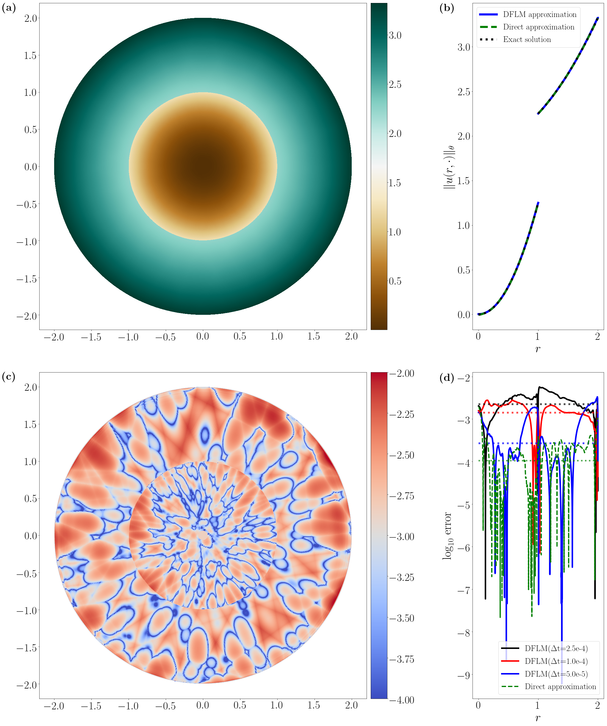
We test our method with $g=1$, $h=1+\frac{1}{4\sigma_{0}}+\frac{3}{4\sigma_{1}}$, $\Delta V=1$, $\sigma_{0}=0.2$, $\sigma_{1}=0.7$, for which the analytic solution is

Note that we do not use the knowledge about the exact function being a radial function and the Cartesian coordinates are used in the input layer. Based on our experiment, the variant of ResNet outperform the MLP and the structure of ResNet with LReLU activation in the first layer activation ($\sigma^{\text{in}}$ defined in Eq. (17)) and SWISH ($\beta=1$) activation in the residual blocks is suitable for this example. In particular, we suspect that the choice of LReLU activation in the first layer is effective for the neural network to represent the multiple functions based on the categorical input variable. The simulation results are presented in Fig. 2. The ResNet described above with 3 identical residual blocks with dimension $[60,60,60,60]$ is trained with $N=2000$ (the number of Brownian walkers), $S=200$ (the number of mini-batch samples on the boundary $\partial\Omega$), $M=200$ (the number of samples for the estimation of the target) by the ADAM optimization method. We measured the accuracy of the neural network approximation using a radial average with $T=10^{4}$ angular samples, $u_{\theta}(r):=\frac{1}{T}\sum\limits_{k=1}^{T}u\left(r\cos\frac{2\pi}{T}k,r\sin\frac{2\pi}{T}k;\theta\right)$, $r\in[0,2]$. We trained the neural network with different time steps $\Delta t$ of the Brownian motion. The neural network approximates the radial dependency of the solution, the jump condition, and the flux continuity condition on the interface, in total, with relative $\mathcal{L}_{2}$-error 2.6975e-4. The details are presented in Fig. 2.

In this section, we consider a quasi-linear elliptic equation used in the modeling of taxis, which is the movement of living systems in response to external stimulus. For example, phototaxis refers to the movement of motile organism toward or away from the source of light, and chemotaxis is the migration of motile cell or organism in a direction affected by the gradient of diffusible substance. The phenomenological equation that describes the steady-state population density $u(x)$ with taxis stimulus $c(x)$ is

in which $D$ is the diffusion coefficient, $G(u,c)$ is the taxis flux, and $H(u)$ is the kinetics of the population. In particular, we choose the taxis flux $G(u,c)$ as $G(u,c)=-\chi u\nabla c$, the diffusive flux of stimulus concentration with a coefficient proportional to the population. This choice of taxis flux is motivated from the model of chemotaxis, known as the Keller-Segel model KSMODEL, KSMODEL2. For given $c(x)$ and $H(x)$, the Bellman equation corresponding to Eq. (45) is

References

- [1] K. Hornik, M. Stinchcombe, H. White, Multilayer feedforward networks are universal approximators, Neural Netw. 2 (5) (1989) 359–366.
- [2] I. E. Lagaris, A. Likas, D. I. Fotiadis, Artificial neural networks for solving ordinary and partial differential equations, IEEE Trans. Neural Netw. 9 (5) (1998) 987–1000.
- [3] E. Weinan, J. Han, A. Jentzen, Deep learning-based numerical methods for high-dimensional parabolic partial differential equations and backward stochastic differential equations, Commun. Math. Stat. 5 (2017) 349–380.
- [4] J. Han, A. Jentzen, E. Weinan, Solving high-dimensional partial differential equations using deep learning, Proc. Natl. Acad. Sci. USA 34 (2018) 8505–8510.
- [5] J. Sirignano, K. Spiliopoulos, DGM: a deep learning algorithm for solving partial differential equations, J. Comput. Phys. 375 (2018) 1339–1364.
- [6] M. Raissi, P. Perdikaris, G. E. Karniadakis, Physics-informed neural networks: a deep learning framework for solving forward and inverse problems involving nonlinear partial differential equations, J. Comput. Phys. 378 (2019) 686–707.
- [7] S. Karumuri, R. Tripathy, I. Bilionis, J. Panchal, Simulator-free solution of high-dimensional stochastic elliptic partial differential equations using deep neural networks, J. Comput. Phys. 404 (2020) 109120.
- [8] M. Raissi, Forward-backward stochastic neural networks: Deep learning of high-dimensional partial differential equations, arXiv:1804.07010.
- [9] M. Raissi, G. E. Karniadakis, Hidden physics models: machine learning of nonlinear partial differential equations, J. Comput. Phys. 357 (2018) 125–141.
- [10] M. Raissi, A. Yazdani, G. E. Karniadakis, Hidden fluid mechanics: A Navier-Stokes informed deep learning framework for assimilating flow visualization data, arXiv:1808.04327.
- [11] M. Raissi, Deep hidden physics models: deep learning of nonlinear partial differential equations, J. Mach. Learn. Res. 19 (1) (2018) 932–955.
- [12] E. Weinan, B. Yu, The deep Ritz method: a deep learning-based numerical algorithm for solving variational problems, Commun. Math. Stat. 6 (1) (2018) 1–12.
- [13] Y. Zhu, N. Zabaras, P.-S. Koutsourelakis, P. Perdikaris, Physics-constrained deep learning for high-dimensional surrogate modeling and uncertainty quantification without labeled data, J. Comput. Phys. 394 (2019) 56–81.
- [14] M. A. Nabian, H. Meidani, A deep learning solution approach for high-dimensional random differential equations, Probabilistic Eng. Mech. 57 (2019) 14–25.
- [15] H. Pham, Continuous-time Stochastic Control and Optimization with Financial Applications, Vol. 61, Springer Science & Business Media, 2009.
- [16] R. S. Sutton, A. G. Barto, Reinforcement Learning: An Introduction, 2nd Edition, The MIT Press, 2018.
- [17] V. Mnih, K. Kavukcuoglu, D. Silver, A. Graves, I. Antonoglou, D. Wierstra, M. Riedmiller, Playing Atari with deep reinforcement learning, arXiv: 1312.5602.
- [18] T. E. Booth, Exact Monte Carlo solution of elliptic partial differential equations, J. Comput. Phys. 39 (2) (1981) 396–404.
- [19] T. E. Booth, Regional Monte Carlo solution of elliptic partial differential equations, J. Comput. Phys. 47 (2) (1982) 281–290.
- [20] J. Delaurentis, L. Romero, A Monte Carlo method for Poisson’s equation, J. Comput. Phys. 90 (1) (1990) 123–140.
- [21] C.-O. Hwang, M. Mascagni, J. A. Given, A Feynman-Kac path-integral implementation for poisson’s equation using an h-conditioned Green’s function, Math. Comput. Simulat. 62 (3-6) (2003) 347–355.
- [22] S. Pauli, R. N. Gantner, P. Arbenz, A. Adelmann, Multilevel Monte Carlo for the Feynman-Kac formula for the Laplace equation, Bit Numer. Math. 55 (2015) 1125–1143.
- [23] I. Karatzas, S. Shreve, Brownian Motion and Stochastic Calculus, 2nd Edition, Springer, 1998.
- [24] C. M. Bishop, Pattern Recognition and Machine Learning, Springer, 2006.
- [25] Y. Goldberg, Neural network methods for natural language processing, Synthesis Lectures on Human Language Technologies 10 (1) (2017) 1–309.
- [26] A. Graves, A.-r. Mohamed, G. Hinton, Speech recognition with deep recurrent neural networks, in: 2013 IEEE international conference on acoustics, speech and signal processing, IEEE, 2013, pp. 6645–6649.
- [27] I. Goodfellow, Y. Bengio, A. Courville, Deep Learning, 2nd Edition, The MIT Press, 2016.
- [28] K. He, X. Zhang, S. Ren, J. Sun, Deep residual learning for image recognition, in: Proceedings of the IEEE conference on computer vision and pattern recognition, 2016, pp. 770–778.
- [29] B. Chang, L. Meng, E. Haber, F. Tung, D. Begert, Multi-level residual networks from dynamical systems view, in: International Conference on Learning Representations, 2018.
- [30] K. Greff, R. K. Srivastava, J. Schmidhuber, Highway and residual networks learn unrolled iterative estimation, in: International Conference on Learning Representations, 2017.
- [31] E. Haber, L. Ruthotto, E. Holtham, S.-H. Jun, Learning across scales - multiscale methods for convolution neural networks, arXiv:1703.02009.
- [32] D. P. Kingma, J. L. Ba, ADAM: a method for stochastic optimization, International Conference on Learning Representations.
- [33] M. Abadi, A. Agarwal, P. Barham, E. Brevdo, Z. Chen, C. Citro, G. S. Corrado, A. Davis, J. Dean, M. Devin, S. Ghemawat, I. Goodfellow, et al., Tensorflow: large-scale machine learning on heterogeneous distributed systems, arXiv:1603.04467.
- [34] W. F. Mitchell, A collection of 2D elliptic problems for testing adaptive algorithms, Appl. Math. Comput. 220 (1) (2013) 350–364.
- [35] P. Ramachandran, B. Zoph, Q. V. Le, Searching for activation functions, arXiv:1710.05941.
- [36] E. F. Keller, L. A. Segel, Initiation of slime mold aggregation viewed as an instability, J. Theor. Biol. 26 (3) (1970) 399–415.
- [37] T. Hillen, K. J. Painter, A user’s guide to PDE models for chemotaxis, J. Math. Biol. (2009) 58–183.
- [38] MATLAB partial differential equation toolbox release 2019b, the MathWorks, Inc., Natick, MA, USA.