跳到论文正文
W Papers独立论文阅读器 arXiv:2001.06128 论文正文 计算阅读时间 · 0%
引用这篇论文根据当前论文元数据生成,正式投稿前建议核对。


License: arXiv.org perpetual non-exclusive license
arXiv:2001.06128v3 [math-ph] 20 May 2021

Coupling constant dependence
for the Schrödinger equation
with an inverse-square potential

A.G. Smirnov Address: I. E. Tamm Theory Department, P. N. Lebedev Physical Institute, Leninsky prospect 53, Moscow 119991, Russia Email address: smirnov@lpi.ru
Abstract.

We consider the one-dimensional Schrödinger equation −f′′+qα​f=E​f-f^{\prime\prime}+q_{\alpha}f=Ef on the positive half-axis with the potential qα​(r)=(α−1/4)​r−2q_{\alpha}(r)=(\alpha-1/4)r^{-2}. It is known that the value α=0\alpha=0 plays a special role in this problem: all self-adjoint realizations of the formal differential expression −∂r2+qα(r)-\partial^{2}_{r}+q_{\alpha}(r) for the Hamiltonian have infinitely many eigenvalues for α<0\alpha<0 and at most one eigenvalue for α≥0\alpha\geq 0. We find a parametrization of self-adjoint boundary conditions and eigenfunction expansions that is analytic in α\alpha and, in particular, is not singular at α=0\alpha=0. Employing suitable singular Titchmarsh–Weyl mm-functions, we explicitly find the spectral measures for all self-adjoint Hamiltonians and prove their smooth dependence on α\alpha and the boundary condition. Using the formulas for the spectral measures, we analyse in detail how the “phase transition” through the point α=0\alpha=0 occurs for both the eigenvalues and the continuous spectrum of the Hamiltonians.

Key words and phrases: 
Schrödinger equation, inverse-square potential, self-adjoint extension, eigenfunction expansion, Titchmarsh-Weyl mm-function

1. Introduction

This paper is devoted to eigenfunction expansions connected with the one-dimensional Schrödinger equation 11 1 The shift of the coupling constant by 1/41/4 in the potential term is a matter of technical convenience: it allows us to get simpler expressions for the solutions of (1.1).

(1.1) −∂r2f(r)+α−1/4r2f(r)=Ef(r),r∈ℝ+,-\partial^{2}_{r}f(r)+\frac{\alpha-1/4}{r^{2}}f(r)=Ef(r),\quad r\in{\mathbb{R}}_{+},

where α\alpha and EE are real parameters and ℝ+{\mathbb{R}}_{+} denotes the positive half-axis (0,∞)(0,\infty).

There are two special values of the coupling constant α\alpha at which this problem undergoes a structural change. One of them is α=1\alpha=1. For α<1\alpha<1, all solutions of (1.1) are square-integrable on the interval (0,a)(0,a) for every a>0a>0. At the same time, only one solution (up to a constant factor) for each EE possesses this property for α≥1\alpha\geq 1. In terms of the well-known Weyl alternative, this means that the differential expression

(1.2) −∂2r+α−1/4r2-\partial^{2}_{r}+\frac{\alpha-1/4}{r^{2}}

corresponds at r=0r=0 to the limit point case for α≥1\alpha\geq 1 and to the limit circle case for α<1\alpha<1. As a consequence, (1.2) has a unique self-adjoint realization in L2​(ℝ+)L_{2}({\mathbb{R}}_{+})22 2 Here and subsequently, we let L2​(ℝ+)L_{2}({\mathbb{R}}_{+}) denote the Hilbert space of (equivalence classes of) square-integrable complex functions on ℝ+{\mathbb{R}}_{+}. for α≥1\alpha\geq 1 and infinitely many self-adjoint realizations in L2​(ℝ+)L_{2}({\mathbb{R}}_{+}) for α<1\alpha<1. The latter correspond to various self-adjoint boundary conditions at r=0r=0.

Another special value of α\alpha is α=0\alpha=0. It has long been known [4, 17] that the spectrum of all self-adjoint realizations of (1.2) is not bounded from below and contains infinitely many negative eigenvalues for α<0\alpha<0. On the other hand, every self-adjoint realization of (1.2) has at most one eigenvalue for α≥0\alpha\geq 0 (the continuous spectrum is [0,∞)[0,\infty) for all real α\alpha).

If κ∈ℝ\kappa\in{\mathbb{R}} and α=κ2\alpha=\kappa^{2}, then the function33 3 In this paper, we use the symbol x\sqrt{x} only for nonnegative xx; the notation z1/2z^{1/2} will be used for a suitable branch of the square root in the complex plane. f⁡(r)=r​Jκ​(E​r)f(r)=\sqrt{r}J_{\kappa}(\sqrt{E}r), where JκJ_{\kappa} is the Bessel function of the first kind of order κ\kappa, is a solution of (1.1) for every E>0E>0 (this follows immediately from the fact that JκJ_{\kappa} satisfies the Bessel equation). These solutions can be used to expand square-integrable functions on ℝ+{\mathbb{R}}_{+}. More precisely, given κ≥0\kappa\geq 0 and a square-integrable complex function ψ\psi on ℝ+{\mathbb{R}}_{+} that vanishes for large rr, we can define the function ψ^\hat{\psi} on ℝ+{\mathbb{R}}_{+} by setting

(1.3) ψ^​(E)=12​∫0∞r​Jκ​(E​r)​ψ​(r)​𝑑r,E>0.\hat{\psi}(E)=\frac{1}{\sqrt{2}}\int_{0}^{\infty}\sqrt{r}J_{\kappa}(\sqrt{E}r)\psi(r)\,dr,\quad E>0.

The map ψ→ψ^\psi\to\hat{\psi} then coincides up to a change of variables with the well-known Hankel transformation [13] and induces a uniquely determined unitary operator in L2​(ℝ+)L_{2}({\mathbb{R}}_{+}). Since the development of a general theory of singular Sturm–Liouville operators by Weyl [27], this transformation has been used by many authors to illustrate various approaches to eigenfunction expansions for problems of this type [28, 24, 18, 10, 9, 16].

For α≥1\alpha\geq 1, transformation (1.3) with κ=α\kappa=\sqrt{\alpha} provides an eigenfunction expansion (i.e., a diagonalizing unitary operator) for the unique self-adjoint realization of (1.2). If 0≤α<10\leq\alpha<1, then it is an eigenfunction expansion for one of infinitely many self-adjoint realizations of (1.2), namely, for the Friedrichs extension of the minimal operator hαh_{\alpha} associated with (1.2) (see [8]; the precise definition of hαh_{\alpha} will be given later in this section). As we shall see, the latter is not bounded from below and, therefore, has no Friedrichs extension for α<0\alpha<0. Accordingly, the right-hand side of (1.3) as a function of α\alpha has a branch point at α=0\alpha=0 and cannot be analytically continued to the region α<0\alpha<0.

For α≥0\alpha\geq 0, eigenfunction expansions corresponding to all self-adjoint realizations of (1.2) were found in [24] (however, without explicitly using the language of operators in Hilbert space). In [17], all self-adjoint Hamiltonians associated with (1.2) and corresponding eigenfunction expansions were constructed for every real α\alpha using the theory of self-adjoint extensions of symmetric operators (a somewhat different treatment of this problem in the framework of self-adjoint extensions can be found in [11, 12]).

The generalized eigenfunctions used in [24, 17, 11, 12] had the same type of branch point singularity at α=0\alpha=0 as that appearing in Hankel transformation (1.3). As a result, the cases 0<α<10<\alpha<1, α=0\alpha=0, and α<0\alpha<0 were treated separately and eigenfunction expansions for α=0\alpha=0 could not be obtained from those for 0<α<10<\alpha<1 and α<0\alpha<0 by taking the limit α→0\alpha\to 0. In [21], we considered problem (1.1) with α=κ2\alpha=\kappa^{2} and constructed a parametrization of self-adjoint realizations of (1.2) and corresponding eigenfunction expansions that is continuous in κ\kappa on the interval (−1,1)(-1,1) (and, in particular, at κ=0\kappa=0). This work was motivated by our previous research [20] of the Aharonov–Bohm model, where zero and nonzero κ\kappa correspond to integer and noninteger values of the dimensionless magnetic flux through the solenoid. In terms of α\alpha, the results of [21] give a continuous transition from the region 0<α<10<\alpha<1 to α=0\alpha=0.

In this paper, we extend the treatment in [21] to also cover the region α<0\alpha<0. We parametrize all eigenfunction expansions associated with (1.2) in such a way that the generalized eigenfunctions turn out to be analytic in α\alpha for α<1\alpha<1, while the corresponding spectral measures are infinitely differentiable in α\alpha on the same interval. Using explicit formulas for the spectral measures, we analyse in detail how the transition through the point α=0\alpha=0 occurs for both the eigenvalues and the continuous spectrum of self-adjoint realizations of (1.2) in this parametrization.

We now give a brief structural description of our results.

For every α∈ℂ\alpha\in{\mathbb{C}}, we define the function qαq_{\alpha} on ℝ+{\mathbb{R}}_{+} by setting

(1.4) qα​(r)=α−1/4r2,r>0.q_{\alpha}(r)=\frac{\alpha-1/4}{r^{2}},\quad r>0.

For real α\alpha, qαq_{\alpha} is the potential term in (1.2).

Let λ+\lambda_{+} be the restriction to ℝ+{\mathbb{R}}_{+} of the Lebesgue measure λ\lambda on ℝ{\mathbb{R}} and 𝒟\mathcal{D} be the space of all complex continuously differentiable functions on ℝ+{\mathbb{R}}_{+} whose derivative is absolutely continuous on ℝ+{\mathbb{R}}_{+} (i.e., absolutely continuous on every segment [a,b][a,b] with 0<a≤b<∞0<a\leq b<\infty). Given α,z∈ℂ\alpha,z\in{\mathbb{C}}, we let ℒα,z\mathscr{L}_{\alpha,z} denote the linear operator from 𝒟\mathcal{D} to the space of complex λ+\lambda_{+}-equivalence classes such that

(1.5) (ℒα,z​f)​(r)=−f′′​(r)+qα​(r)​f​(r)−z​f​(r)(\mathscr{L}_{\alpha,z}f)(r)=-f^{\prime\prime}(r)+q_{\alpha}(r)f(r)-zf(r)

for λ\lambda-a.e.44 4 Throughout the paper, a.e. means either “almost every” or “almost everywhere.” r∈ℝ+r\in{\mathbb{R}}_{+} and set

(1.6) ℒα=ℒα,0.\mathscr{L}_{\alpha}=\mathscr{L}_{\alpha,0}.

Let α∈ℝ\alpha\in{\mathbb{R}}. We define the linear subspace Δα\Delta_{\alpha} of 𝒟\mathcal{D} by setting

(1.7) Δα={f∈𝒟:f​ and ​ℒα​f​ are both square-integrable on ​ℝ+}.\Delta_{\alpha}=\{f\in\mathcal{D}:f\mbox{ and }\mathscr{L}_{\alpha}f\mbox{ are both square-integrable on }{\mathbb{R}}_{+}\}.

For every linear subspace ZZ of Δα\Delta_{\alpha}, let Hα​(Z)H_{\alpha}(Z) be the linear operator in L2​(ℝ+)L_{2}({\mathbb{R}}_{+}) defined by the relations55 5 Here and subsequently, we let DFD_{F} denote the domain of definition of a map FF.

(1.8) DHα​(Z)={[f]:f∈Z},Hα(Z)[f]=ℒαf,f∈Z,\begin{split}&D_{H_{\alpha}(Z)}=\{[f]:f\in Z\},\\ &H_{\alpha}(Z)[f]=\mathscr{L}_{\alpha}f,\quad f\in Z,\end{split}

where [f]=[f]λ+[f]=[f]_{\lambda_{+}} denotes the λ+\lambda_{+}-equivalence class of ff. We clearly have C0∞​(ℝ+)⊂ΔαC_{0}^{\infty}({\mathbb{R}}_{+})\subset\Delta_{\alpha}, where C0∞​(ℝ+)C_{0}^{\infty}({\mathbb{R}}_{+}) is the space of all smooth functions on ℝ+{\mathbb{R}}_{+} with compact support. The operator

(1.9) hˇα=Hα​(C0∞​(ℝ+))\check{h}_{\alpha}=H_{\alpha}(C_{0}^{\infty}({\mathbb{R}}_{+}))

is obviously symmetric and, hence, closable. The closure of hˇα\check{h}_{\alpha} is denoted by hαh_{\alpha},

(1.10) hα=hˇα¯.h_{\alpha}=\overline{\check{h}_{\alpha}}.

We shall see that the adjoint hα∗h_{\alpha}^{*} of hαh_{\alpha} is given by

(1.11) hα∗=Hα​(Δα).h_{\alpha}^{*}=H_{\alpha}(\Delta_{\alpha}).

If TT is a symmetric extension of hαh_{\alpha}, then hα∗h^{*}_{\alpha} is an extension of T∗T^{*} and hence of TT. By (1.11), we conclude that TT is of the form Hα​(Z)H_{\alpha}(Z) for some subspace ZZ of Δα\Delta_{\alpha}.

Self-adjoint operators of the form Hα​(Z)H_{\alpha}(Z) can be naturally viewed as self-adjoint realizations of differential expression (1.2). If Hα​(Z)H_{\alpha}(Z) is self-adjoint, then equality (1.11) and the closedness of hαh_{\alpha} imply that Hα​(Z)H_{\alpha}(Z) is an extension of hαh_{\alpha} because Hα​(Δα)H_{\alpha}(\Delta_{\alpha}) is an extension of Hα​(Z)H_{\alpha}(Z). Therefore, the self-adjoint realizations of (1.2) are precisely the self-adjoint extensions of hαh_{\alpha} (or, equivalently, of hˇα\check{h}_{\alpha}).

For every α,z∈ℂ\alpha,z\in{\mathbb{C}}, we shall construct real-analytic functions 𝒜α​(z)\mathcal{A}^{\alpha}(z) and ℬα​(z)\mathcal{B}^{\alpha}(z) on ℝ+{\mathbb{R}}_{+} such that

(1.12) ℒα,z​𝒜α​(z)=ℒα,z​ℬα​(z)=0,α,z∈ℂ.\mathscr{L}_{\alpha,z}\mathcal{A}^{\alpha}(z)=\mathscr{L}_{\alpha,z}\mathcal{B}^{\alpha}(z)=0,\quad\alpha,z\in{\mathbb{C}}.

The functions 𝒜α​(z)\mathcal{A}^{\alpha}(z) and ℬα​(z)\mathcal{B}^{\alpha}(z) are real for real α\alpha and zz. Moreover, the quantities66 6 Given a map FF whose values are also maps, we let F⁡(x|y)F(x|y) denote the value of F⁡(x)F(x) at a point yy: F​(x|y)=(F​(x))​(y)F(x|y)=(F(x))(y). 𝒜α​(z|r)\mathcal{A}^{\alpha}(z|r) and ℬα​(z|r)\mathcal{B}^{\alpha}(z|r) are entire analytic in α\alpha and zz for every fixed r>0r>0 and, in particular, are not singular at α=0\alpha=0. If α<1\alpha<1 and z∈ℂz\in{\mathbb{C}}, then 𝒜α​(z)\mathcal{A}^{\alpha}(z) and ℬα​(z)\mathcal{B}^{\alpha}(z) are linear independent and are both square-integrable on the interval (0,a)(0,a) for every a>0a>0 (as mentioned above, we have the limit circle case for α<1\alpha<1).

Given f,g∈𝒟f,g\in\mathcal{D}, we let Wr​(f,g)W_{r}(f,g) denote the Wronskian of ff and gg at a point r>0r>0,

(1.13) Wr​(f,g)=f⁡(r)​g′​(r)−f′​(r)​g​(r).W_{r}(f,g)=f(r)g^{\prime}(r)-f^{\prime}(r)g(r).

Clearly, r→Wr​(f,g)r\to W_{r}(f,g) is an absolutely continuous function on ℝ+{\mathbb{R}}_{+}.

For every α,ϑ,z∈ℂ\alpha,\vartheta,z\in{\mathbb{C}}, we define the function 𝒰ϑα​(z)\mathcal{U}^{\alpha}_{\vartheta}(z) on ℝ+{\mathbb{R}}_{+} by the relation

(1.14) 𝒰ϑα​(z)=𝒜α​(z)​cos⁡ϑ+ℬα​(z)​sin⁡ϑ.\mathcal{U}^{\alpha}_{\vartheta}(z)=\mathcal{A}^{\alpha}(z)\cos\vartheta+\mathcal{B}^{\alpha}(z)\sin\vartheta.

By (1.12), we obviously have

(1.15) ℒα,z​𝒰ϑα​(z)=0,α,ϑ,z∈ℂ.\mathscr{L}_{\alpha,z}\mathcal{U}^{\alpha}_{\vartheta}(z)=0,\quad\alpha,\vartheta,z\in{\mathbb{C}}.

The properties of 𝒜α​(z)\mathcal{A}^{\alpha}(z) and ℬα​(z)\mathcal{B}^{\alpha}(z) imply that 𝒰ϑα​(z)\mathcal{U}^{\alpha}_{\vartheta}(z) is real for real α,ϑ\alpha,\vartheta, and zz and the quantity 𝒰ϑα​(z|r)\mathcal{U}^{\alpha}_{\vartheta}(z|r) is entire analytic in α,ϑ\alpha,\vartheta, and zz for every fixed r>0r>0. If α<1\alpha<1, then 𝒰ϑα​(z)\mathcal{U}^{\alpha}_{\vartheta}(z) is nontrivial for every ϑ,z∈ℂ\vartheta,z\in{\mathbb{C}}. We shall show that limr↓0Wr​(𝒰ϑα​(z),𝒰ϑα​(z′))=0\lim_{r\downarrow 0}W_{r}(\mathcal{U}^{\alpha}_{\vartheta}(z),\mathcal{U}^{\alpha}_{\vartheta}(z^{\prime}))=0 for all α<1\alpha<1, ϑ∈ℝ\vartheta\in{\mathbb{R}}, and z,z′∈ℂz,z^{\prime}\in{\mathbb{C}}. This condition means that 𝒰ϑα​(z|r)\mathcal{U}^{\alpha}_{\vartheta}(z|r) for various zz have the same asymptotics as r↓0r\downarrow 0.

Let f∈𝒟f\in\mathcal{D} and α,ϑ,z∈ℂ\alpha,\vartheta,z\in{\mathbb{C}}. In view of (1.15), integration by parts yields

∫ra(ℒα,z​f)​(r′)​𝒰ϑα​(z|r′)​d​r′=Wr​(𝒰ϑα​(z),f)−Wa​(𝒰ϑα​(z),f)\int_{r}^{a}(\mathscr{L}_{\alpha,z}f)(r^{\prime})\mathcal{U}^{\alpha}_{\vartheta}(z|r^{\prime})\,dr^{\prime}=W_{r}(\mathcal{U}^{\alpha}_{\vartheta}(z),f)-W_{a}(\mathcal{U}^{\alpha}_{\vartheta}(z),f)

for every a,r>0a,r>0. If α<1\alpha<1, then 𝒰ϑα​(z)\mathcal{U}^{\alpha}_{\vartheta}(z) is square-integrable on (0,a)(0,a) for every a>0a>0 and this equality implies that Wr​(𝒰ϑα​(z),f)W_{r}(\mathcal{U}^{\alpha}_{\vartheta}(z),f) has a limit as r↓0r\downarrow 0 for every ϑ,z∈ℂ\vartheta,z\in{\mathbb{C}} and f∈Δαf\in\Delta_{\alpha}. Given α<1\alpha<1 and ϑ∈ℝ\vartheta\in{\mathbb{R}}, we define the operator hα,ϑh_{\alpha,\vartheta} in L2​(ℝ+)L_{2}({\mathbb{R}}_{+}) by the relation

(1.16) hα,ϑ=Hα​(Zα,ϑ),h_{\alpha,\vartheta}=H_{\alpha}(Z_{\alpha,\vartheta}),

where the linear subspace Zα,ϑZ_{\alpha,\vartheta} of Δα\Delta_{\alpha} is given by

(1.17) Zα,ϑ={f∈Δα:limr↓0Wr​(𝒰ϑα​(0),f)=0}.Z_{\alpha,\vartheta}=\{f\in\Delta_{\alpha}:\lim_{r\downarrow 0}W_{r}(\mathcal{U}^{\alpha}_{\vartheta}(0),f)=0\}.

By (1.14) and the definition of hα,ϑh_{\alpha,\vartheta}, we have

(1.18) hα,ϑ+π=hα,ϑ,α<1,ϑ∈ℝ.h_{\alpha,\vartheta+\pi}=h_{\alpha,\vartheta},\quad\alpha<1,\,\vartheta\in{\mathbb{R}}.

The next statement gives a complete description of the self-adjoint extensions of hαh_{\alpha} for every α∈ℝ\alpha\in{\mathbb{R}}.

Theorem 1.1.

For α≥1\alpha\geq 1, the operator hαh_{\alpha} is self-adjoint. If α<1\alpha<1, then hα,ϑh_{\alpha,\vartheta} is a self-adjoint extension of hαh_{\alpha} for every ϑ∈ℝ\vartheta\in{\mathbb{R}} and, conversely, every self-adjoint extension of hαh_{\alpha} is equal to hα,ϑh_{\alpha,\vartheta} for some ϑ∈ℝ\vartheta\in{\mathbb{R}}. Given ϑ,ϑ′∈ℝ\vartheta,\vartheta^{\prime}\in{\mathbb{R}}, we have hα,ϑ=hα,ϑ′h_{\alpha,\vartheta}=h_{\alpha,\vartheta^{\prime}} if and only if ϑ−ϑ′∈π​ℤ\vartheta-\vartheta^{\prime}\in\pi{\mathbb{Z}}.

As will be obvious from the explicit definitions of 𝒜α​(z)\mathcal{A}^{\alpha}(z) and ℬα​(z)\mathcal{B}^{\alpha}(z) in Sec. 2, these functions are actually square integrable on intervals (0,a)(0,a) with a>0a>0 for all α\alpha belonging to the domain

Π={α∈ℂ:α=κ2​ for some κ∈ℂ such that ​|Re​κ|<1}.\Pi=\{\alpha\in{\mathbb{C}}:\alpha=\kappa^{2}\mbox{ for some $\kappa\in{\mathbb{C}}$ such that }|\mathrm{Re}\,\kappa|<1\}.\

and all z∈ℂz\in{\mathbb{C}}. Hence, the above definition of hα,ϑh_{\alpha,\vartheta} can be naturally extended to all α∈Π\alpha\in\Pi and ϑ∈ℂ\vartheta\in{\mathbb{C}}. Moreover, it is possible to show that such an extended family of operators is holomorphic on Π×ℂ\Pi\times{\mathbb{C}} in the sense of Kato (see Ch. 7 in [14]) and, therefore, hα,ϑh_{\alpha,\vartheta} with α<1\alpha<1 and ϑ∈ℝ\vartheta\in{\mathbb{R}} constitute a real-analytic family of operators. This can be proved using a technique similar to that employed in [3] for the case of extensions of hαh_{\alpha} homogeneous with respect to dilations of ℝ+{\mathbb{R}}_{+}. The spectral analysis of a holomorphic family similar to hα,ϑh_{\alpha,\vartheta} can be found in [6], where, however, κ\kappa rather than α\alpha was used as a parameter and the case α=0\alpha=0 was treated separately (see also [5] for an analogous treatment of the Coulomb potential; a possibility of removing the singularity at κ=0\kappa=0 was indicated in Remark 2.5 in [6]). However, the analysis of hα,ϑh_{\alpha,\vartheta} for complex α\alpha and ϑ\vartheta is beyond the scope of this paper. In the sequel, we confine ourselves to the self-adjoint case α<1\alpha<1, ϑ∈ℝ\vartheta\in{\mathbb{R}}.

Given a positive Borel measure ν\nu on ℝ{\mathbb{R}} and a ν\nu-measurable complex function gg, we let 𝒯gν\mathcal{T}^{\nu}_{g} denote the operator of multiplication by gg in the Hilbert space L2​(ℝ,ν)L_{2}({\mathbb{R}},\nu) of ν\nu-square-integrable complex functions on ℝ{\mathbb{R}}.77 7 More precisely, 𝒯gν\mathcal{T}^{\nu}_{g} is the operator in L2​(ℝ,ν)L_{2}({\mathbb{R}},\nu) whose graph consists of all pairs (φ1,φ2)(\varphi_{1},\varphi_{2}) such that φ1,φ2∈L2​(ℝ,ν)\varphi_{1},\varphi_{2}\in L_{2}({\mathbb{R}},\nu) and φ2​(E)=g⁡(E)​φ1​(E)\varphi_{2}(E)=g(E)\varphi_{1}(E) for ν\nu-a.e. EE. If gg is real, then 𝒯gν\mathcal{T}^{\nu}_{g} is self-adjoint. We let L2c​(ℝ+)L_{2}^{c}({\mathbb{R}}_{+}) denote the subspace of L2​(ℝ+)L_{2}({\mathbb{R}}_{+}) consisting of all its elements vanishing λ\lambda-a.e. outside some compact subset of ℝ+{\mathbb{R}}_{+}.

It turns out that the functions 𝒰ϑα​(E)\mathcal{U}^{\alpha}_{\vartheta}(E) with real EE can be used as generalized eigenfunctions for constructing eigenfunction expansions for hα,ϑh_{\alpha,\vartheta}. More precisely, for every α<1\alpha<1 and ϑ∈ℝ\vartheta\in{\mathbb{R}}, we shall construct a positive Radon measure88 8 We recall that a Borel measure ν\nu on ℝ{\mathbb{R}} is called a Radon measure on ℝ{\mathbb{R}} if ν⁡(K)<∞\nu(K)<\infty for every compact set K⊂ℝK\subset{\mathbb{R}}. 𝒱α,ϑ\mathcal{V}_{\alpha,\vartheta} on ℝ{\mathbb{R}} such that

(1.19) ∫ℝd​𝒱α,ϑ​(E)E2+1<∞\int_{\mathbb{R}}\frac{d\mathcal{V}_{\alpha,\vartheta}(E)}{E^{2}+1}<\infty

and the following statement holds.

Theorem 1.2.

Let α<1\alpha<1 and ϑ∈ℝ\vartheta\in{\mathbb{R}}. Then there is a unique unitary operator Uα,ϑ:L2​(ℝ+)→L2​(ℝ,𝒱α,ϑ)U_{\alpha,\vartheta}\colon L_{2}({\mathbb{R}}_{+})\to L_{2}({\mathbb{R}},\mathcal{V}_{\alpha,\vartheta}) such that

(Uα,ϑ​ψ)​(E)=∫0∞𝒰ϑα​(E|r)​ψ​(r)​𝑑r,ψ∈L2c​(ℝ+),(U_{\alpha,\vartheta}\psi)(E)=\int_{0}^{\infty}\mathcal{U}^{\alpha}_{\vartheta}(E|r)\psi(r)\,dr,\quad\psi\in L_{2}^{c}({\mathbb{R}}_{+}),

for 𝒱α,ϑ\mathcal{V}_{\alpha,\vartheta}-a.e. EE, and we have

(1.20) hα,ϑ=Uα,ϑ−1​𝒯ι𝒱α,ϑ​Uα,ϑ,h_{\alpha,\vartheta}=U_{\alpha,\vartheta}^{-1}\mathcal{T}^{\mathcal{V}_{\alpha,\vartheta}}_{\iota}U_{\alpha,\vartheta},

where ι\iota is the identity function on ℝ{\mathbb{R}} (i.e., ι⁡(E)=E\iota(E)=E for all E∈ℝE\in{\mathbb{R}}).

Clearly, the measures 𝒱α,ϑ\mathcal{V}_{\alpha,\vartheta} (which will be referred to as the spectral measures) contain all information about the spectral properties of the operators hα,ϑh_{\alpha,\vartheta}. In particular, E∈ℝE\in{\mathbb{R}} is an eigenvalue of hα,ϑh_{\alpha,\vartheta} if and only if the measure 𝒱α,ϑ\mathcal{V}_{\alpha,\vartheta} of the one-point set {E}\{E\} is strictly positive. In agreement with (1.14) and (1.18), 𝒱α,ϑ\mathcal{V}_{\alpha,\vartheta} is π\pi-periodic in ϑ\vartheta,

(1.21) 𝒱α,ϑ+π=𝒱α,ϑ,α<1,ϑ∈ℝ.\mathcal{V}_{\alpha,\vartheta+\pi}=\mathcal{V}_{\alpha,\vartheta},\quad\alpha<1,\,\vartheta\in{\mathbb{R}}.

Let ω\omega be the π\pi-periodic function on ℝ{\mathbb{R}} such that

(1.22) ω⁡(ϑ)=(1−2​|ϑ|π)2,−π2≤ϑ≤π2.\omega(\vartheta)=\left(1-\frac{2|\vartheta|}{\pi}\right)^{2},\quad-\frac{\pi}{2}\leq\vartheta\leq\frac{\pi}{2}.

Clearly, we have 0≤ω⁡(ϑ)≤10\leq\omega(\vartheta)\leq 1 for all ϑ∈ℝ\vartheta\in{\mathbb{R}}. We define the subsets Q0Q_{0}, Q1Q_{1}, and Q∞Q_{\infty} of ℝ2{\mathbb{R}}^{2} by the relations (see Fig. 1)

(1.23) Q0={(α,ϑ)∈ℝ2:ω⁡(ϑ)≤α<1},\displaystyle Q_{0}=\{(\alpha,\vartheta)\in{\mathbb{R}}^{2}:\omega(\vartheta)\leq\alpha<1\},
(1.24) Q1={(α,ϑ)∈ℝ2:0≤α<ω⁡(ϑ)},\displaystyle Q_{1}=\{(\alpha,\vartheta)\in{\mathbb{R}}^{2}:0\leq\alpha<\omega(\vartheta)\},
(1.25) Q∞={(α,ϑ)∈ℝ2:α<0}.\displaystyle Q_{\infty}=\{(\alpha,\vartheta)\in{\mathbb{R}}^{2}:\alpha<0\}.

The analysis of the measures 𝒱α,ϑ\mathcal{V}_{\alpha,\vartheta} shows that hα,ϑh_{\alpha,\vartheta} has no eigenvalues for (α,ϑ)∈Q0(\alpha,\vartheta)\in Q_{0}, one eigenvalue for (α,ϑ)∈Q1(\alpha,\vartheta)\in Q_{1}, and infinitely many eigenvalues that are not bounded from below for (α,ϑ)∈Q∞(\alpha,\vartheta)\in Q_{\infty}. Using a parametrization of generalized eigenfunctions that is analytic on the entire domain

(1.26) Q=Q0∪Q1∪Q∞={(α,ϑ)∈ℝ2:α<1}Q=Q_{0}\cup Q_{1}\cup Q_{\infty}=\{(\alpha,\vartheta)\in{\mathbb{R}}^{2}:\alpha<1\}

allows us to understand in detail what happens to eigenvalues as we pass from Q∞Q_{\infty} to Q1Q_{1} through the line α=0\alpha=0. It turns out that there is one eigenvalue that crosses this line in an analytic manner, while the rest infinitely many eigenvalues tend either to −∞-\infty or to zero as α↑0\alpha\uparrow 0 and die away there. Moreover, the density of 𝒱α,ϑ\mathcal{V}_{\alpha,\vartheta} corresponding to the continuous part of the spectrum turns out to be real-analytic on QQ.

If α<0\alpha<0, then the operator hαh_{\alpha} is not bounded from below because otherwise it would have self-adjoint extensions (e.g., its Friedrichs extension) that are bounded from below, in contradiction to Theorem 1.1 and the described properties of eigenvalues of hα,ϑh_{\alpha,\vartheta} for (α,ϑ)∈Q∞(\alpha,\vartheta)\in Q_{\infty}. On the other hand, it is easy to see that hαh_{\alpha} is positive for α≥0\alpha\geq 0. Indeed, let f∈C0∞​(ℝ+)f\in C_{0}^{\infty}({\mathbb{R}}_{+}), ψ=[f]\psi=[f], and ϱ\varrho be a real number. Using the integration by parts, we easily derive from (1.9) that

⟨ψ,hˇα​ψ⟩=∫0∞r2​ϱ​(|∂rf~​(r)|2+α−1/4−ϱ2+ϱr2​|f~​(r)|2)​𝑑r,\langle\psi,\check{h}_{\alpha}\psi\rangle=\int_{0}^{\infty}r^{2\varrho}\left(|\partial_{r}\tilde{f}(r)|^{2}+\frac{\alpha-1/4-\varrho^{2}+\varrho}{r^{2}}|\tilde{f}(r)|^{2}\right)dr,

where ⟨⋅,⋅⟩\langle\cdot,\cdot\rangle is the scalar product in L2​(ℝ+)L_{2}({\mathbb{R}}_{+}) and the function f~\tilde{f} on ℝ+{\mathbb{R}}_{+} is given by f~​(r)=r−ϱ​f​(r)\tilde{f}(r)=r^{-\varrho}f(r), r>0r>0. The maximum of −ϱ2+ϱ-\varrho^{2}+\varrho is attained at ϱ=1/2\varrho=1/2 and is equal to 1/41/4. Substituting this value to the above equality, we deduce that ⟨ψ,hˇα​ψ⟩≥0\langle\psi,\check{h}_{\alpha}\psi\rangle\geq 0 for all α≥0\alpha\geq 0 and ψ∈Dhˇα\psi\in D_{\check{h}_{\alpha}}. The positivity of hαh_{\alpha} for α≥0\alpha\geq 0 now follows from (1.10).

Refer to caption
Figure 1. The sets Q0Q_{0}, Q1Q_{1}, and Q∞Q_{\infty} are represented by white, dark gray, and light gray regions respectively.

It seems probable that the dependence of 𝒱α,ϑ\mathcal{V}_{\alpha,\vartheta} on α\alpha and ϑ\vartheta is not analytic at the boundaries between the regions Q0Q_{0}, Q1Q_{1}, and Q∞Q_{\infty}, where eigenvalues arise and disappear (however, we do not prove this claim in this paper). At the same time, we shall show that this dependence is smooth on QQ in a suitable sense. To formulate this result precisely, we make use of the Schwartz space 𝒮\mathscr{S} of rapidly decreasing smooth functions. More specifically, 𝒮\mathscr{S} consists of all infinitely differentiable functions φ\varphi on ℝ{\mathbb{R}} such that

supE∈ℝ,k∈{0,…,n}|φ(k)​(E)|​(1+|E|)n<∞\sup_{E\in{\mathbb{R}},\,k\in\{0,\ldots,n\}}|\varphi^{(k)}(E)|(1+|E|)^{n}<\infty

for every nonnegative integer nn, where φ(k)\varphi^{(k)} stands for the kkth derivative of φ\varphi. The space 𝒮\mathscr{S} is widely used in the theory of generalized functions as the test function space for tempered distributions. In view of (1.19), every φ∈𝒮\varphi\in\mathscr{S} is 𝒱α,ϑ\mathcal{V}_{\alpha,\vartheta}-integrable for all α<1\alpha<1 and ϑ∈ℝ\vartheta\in{\mathbb{R}}.

Theorem 1.3.

For every φ∈𝒮\varphi\in\mathscr{S}, the function (α,ϑ)→∫φ⁡(E)​d​𝒱α,ϑ​(E)(\alpha,\vartheta)\to\int\varphi(E)\,d\mathcal{V}_{\alpha,\vartheta}(E) is infinitely differentiable on the domain QQ given by (1.26)(\ref{domain}).

Thus, our construction of eigenfunction expansions is, as a whole, at least infinitely differentiable.

When considering equation (1.1), it is convenient to set α=κ2\alpha=\kappa^{2} and find its solutions as functions of κ\kappa (we have actually done so in the case of Hankel transformation (1.3)). To return to the initial variable α\alpha, it is then necessary to replace κ\kappa with the square root of α\alpha. As was discussed above, this may lead to the appearance of branch points and the loss of analyticity. This does not happen, however, if the solution in question is an even holomorphic function of κ\kappa. Indeed, suppose we have an even holomorphic function gg, which will be assumed for simplicity to be entire. Then gg has the power series expansion of the form g⁡(w)=∑k=0∞ck​w2​kg(w)=\sum_{k=0}^{\infty}c_{k}w^{2k} for every w∈ℂw\in{\mathbb{C}}. If we define the entire analytic function GG by the formula G⁡(ζ)=∑k=0∞ck​ζkG(\zeta)=\sum_{k=0}^{\infty}c_{k}\zeta^{k}, ζ∈ℂ\zeta\in{\mathbb{C}}, then we have

(1.27) G⁡(w2)=g⁡(w)G(w^{2})=g(w)

for all w∈ℂw\in{\mathbb{C}} and, hence, G⁡(ζ)G(\zeta) can be viewed as a result of “substituting the square root of ζ\zeta” in gg. More generally, representations of type (1.27) can be obtained for even holomorphic functions on arbitrary reflection-symmetric domains and for the case of several complex variables (see Appendix A). Our construction of the solutions 𝒜α​(z)\mathcal{A}^{\alpha}(z) and ℬα​(z)\mathcal{B}^{\alpha}(z) is based on the described technique. We shall first find functions 𝔞κ​(z)\mathfrak{a}^{\kappa}(z) and 𝔟κ​(z)\mathfrak{b}^{\kappa}(z) that are even in κ\kappa and satisfy (1.1) with α\alpha and EE replaced with κ2\kappa^{2} and zz respectively and then define 𝒜α​(z)\mathcal{A}^{\alpha}(z) and ℬα​(z)\mathcal{B}^{\alpha}(z) by requiring that 𝒜κ2​(z)=𝔞κ​(z)\mathcal{A}^{\kappa^{2}}(z)=\mathfrak{a}^{\kappa}(z) and ℬκ2​(z)=𝔟κ​(z)\mathcal{B}^{\kappa^{2}}(z)=\mathfrak{b}^{\kappa}(z) for every κ,z∈ℂ\kappa,z\in{\mathbb{C}}.

Simple examples of representations of type (1.27), which will be important for us, are obtained if we choose gg to be equal either to the cosine or the entire function sinc\sinc that is defined by the formula

sincw={w−1​sin⁡w,w∈ℂ∖{0},1,w=0.\sinc w=\left\{\begin{matrix}w^{-1}\sin w,&w\in{\mathbb{C}}\setminus\{0\},\\ 1,&w=0.\end{matrix}\right.

Proceeding as above, we find that

(1.28) cos⁡w=Cos⁡(w2),sinc⁡w=Sinc⁡(w2)\cos w=\Cos(w^{2}),\quad\sinc w=\Sinc(w^{2})

for every w∈ℂw\in{\mathbb{C}}, where the entire functions Cos\Cos and Sinc\Sinc are given by

(1.29) Cos⁡ζ=∑k=0∞(−ζ)k(2​k)!,Sinc⁡ζ=∑k=0∞(−ζ)k(2​k+1)!,ζ∈ℂ.\Cos\zeta=\sum_{k=0}^{\infty}\frac{(-\zeta)^{k}}{(2k)!},\quad\Sinc\zeta=\sum_{k=0}^{\infty}\frac{(-\zeta)^{k}}{(2k+1)!},\quad\zeta\in{\mathbb{C}}.

It follows from (1.28) that

(1.30) Cos⁡(−w2)=cos⁡(i​w)=ch⁡w,w​Sinc⁡(−w2)=w​sinc⁡(i​w)=sh⁡w\Cos(-w^{2})=\cos(iw)=\ch w,\quad w\Sinc(-w^{2})=w\sinc(iw)=\sh w

for every w∈ℂw\in{\mathbb{C}}. In particular, we have

(1.31) Cos⁡ξ=cos⁡(ξ),Sinc⁡ξ=sinc⁡(ξ),ξ≥0,\displaystyle\Cos\xi=\cos(\sqrt{\xi}),\quad\Sinc\xi=\sinc(\sqrt{\xi}),\quad\xi\geq 0,
(1.32) Cosξ=ch(|ξ|),Sincξ=|ξ|−1/2sh(|ξ|),ξ<0.\displaystyle\Cos\xi=\ch(\sqrt{|\xi|}),\quad\Sinc\xi=|\xi|^{-1/2}\sh(\sqrt{|\xi|}),\quad\xi<0.

The graphs of Cos⁡ξ\Cos\xi and Sinc⁡ξ\Sinc\xi are shown in Fig. 2.

Refer to caption
Figure 2. Solid and dashed lines correspond to the functions Cos\Cos and Sinc\Sinc respectively.

Formulas (1.31) and (1.32) show that, in spite of being analytic, the functions Cos\Cos and Sinc\Sinc are expressed in a piecewise way in terms of the standard trigonometric and hyperbolic functions. We shall see that various quantities related to the spectral measures (such as eigenvalues and the density of the absolutely continuous part of 𝒱α,ϑ\mathcal{V}_{\alpha,\vartheta}) can be conveniently expressed through Cos\Cos and Sinc\Sinc. Accordingly, the formulas for these quantities in terms of the ordinary elementary functions are of a piecewise nature. This suggests that Cos\Cos and Sinc\Sinc are more suitable as “elementary functions” for our problem. Some properties of these functions that will be necessary for us are summarized in Appendix B.

The paper is organized as follows. In Sec. 2, we define the solutions 𝒜α​(z)\mathcal{A}^{\alpha}(z) and ℬα​(z)\mathcal{B}^{\alpha}(z) and the spectral measures 𝒱α,ϑ\mathcal{V}_{\alpha,\vartheta}, thus completing the formulation of our results. The definition of the measures 𝒱α,ϑ\mathcal{V}_{\alpha,\vartheta} in Sec. 2 is given via Herglotz representations (see Appendix C) of suitable holomorphic functions in the upper complex half-plane and is not quite explicit. In Sec. 3, we obtain concrete formulas for the point and absolutely continuous parts of 𝒱α,ϑ\mathcal{V}_{\alpha,\vartheta}. In particular, this allows us to justify the “phase diagram” in Fig. 1 and analyze the dependence of eigenvalues of hα,ϑh_{\alpha,\vartheta} on α\alpha and ϑ\vartheta. In Sec. 4, we recall the general theory concerning self-adjoint extensions of one-dimensional Schrödinger operators and apply it to the proof of Theorem 1.1. Our treatment of eigenfunction expansions relies on the method of singular Titchmarsh–Weyl mm-functions [16]. In Sec. 5, we briefly describe this method and then use it to prove Theorem 1.2. Sec. 6 is devoted to the proof of Theorem 1.3.

2. Definition of generalized eigenfunctions and spectral measures

2.1. Definition of 𝒜α​(z)\mathcal{A}^{\alpha}(z) and ℬα​(z)\mathcal{B}^{\alpha}(z).

For any z,κ∈ℂz,\kappa\in{\mathbb{C}}, we define the function 𝔲κ​(z)\mathfrak{u}^{\kappa}(z) on ℝ+{\mathbb{R}}_{+} by the relation

(2.1) 𝔲κ​(z|r)=r1/2+κ​𝒳κ​(r2​z),r>0,\mathfrak{u}^{\kappa}(z|r)=r^{1/2+\kappa}\mathcal{X}_{\kappa}(r^{2}z),\quad r>0,

where the entire function 𝒳κ\mathcal{X}_{\kappa} is given by

(2.2) 𝒳κ​(ζ)=12κ​∑n=0∞(−1)n​ζnΓ⁡(κ+n+1)​n!​22​n,ζ∈ℂ.\mathcal{X}_{\kappa}(\zeta)=\frac{1}{2^{\kappa}}\sum_{n=0}^{\infty}\frac{(-1)^{n}\zeta^{n}}{\Gamma(\kappa+n+1)n!2^{2n}},\quad\zeta\in{\mathbb{C}}.

The function 𝒳κ\mathcal{X}_{\kappa} is closely related to Bessel functions: for ζ≠0\zeta\neq 0, we have

(2.3) 𝒳κ(ζ)=ζ−κ/2Jκ(ζ1/2).\mathcal{X}_{\kappa}(\zeta)=\zeta^{-\kappa/2}J_{\kappa}(\zeta^{1/2}).

Because JκJ_{\kappa} satisfies the Bessel equation, it follows that

(2.4) −∂r2𝔲±κ(z|r)+κ2−1/4r2𝔲±κ(z|r)=z𝔲±κ(z|r),r>0,-\partial^{2}_{r}\mathfrak{u}^{\pm\kappa}(z|r)+\frac{\kappa^{2}-1/4}{r^{2}}\mathfrak{u}^{\pm\kappa}(z|r)=z\mathfrak{u}^{\pm\kappa}(z|r),\quad r>0,

for every κ∈ℂ\kappa\in{\mathbb{C}} and z≠0z\neq 0. By continuity, this is also true for z=0z=0. We therefore have

(2.5) ℒκ2,z​𝔲±κ​(z)=0,κ,z∈ℂ.\mathscr{L}_{\kappa^{2},z}\mathfrak{u}^{\pm\kappa}(z)=0,\quad\kappa,z\in{\mathbb{C}}.

For every κ,z∈ℂ\kappa,z\in{\mathbb{C}}, we define the function 𝔞κ​(z)\mathfrak{a}^{\kappa}(z) on ℝ+{\mathbb{R}}_{+} by setting

(2.6) 𝔞κ(z)=𝔲κ​(z)−𝔲−κ​(z)κcosϑκ,κ∈ℂ∖{0},\mathfrak{a}^{\kappa}(z)=\frac{\mathfrak{u}^{\kappa}(z)-\mathfrak{u}^{-\kappa}(z)}{\kappa}\cos\vartheta_{\kappa},\quad\kappa\in{\mathbb{C}}\setminus\{0\},

and

(2.7) 𝔞0​(z|r)=limκ→0𝔞κ​(z|r)=2​[(ln⁡r2+γ)​𝔲0​(z|r)−r​𝒴​(r2​z)],r>0,\mathfrak{a}^{0}(z|r)=\lim_{\kappa\to 0}\mathfrak{a}^{\kappa}(z|r)=2\left[\left(\ln\frac{r}{2}+\gamma\right)\mathfrak{u}^{0}(z|r)-\sqrt{r}\,\mathcal{Y}(r^{2}z)\right],\quad r>0,

where

(2.8) ϑκ=π​κ2,\vartheta_{\kappa}=\frac{\pi\kappa}{2},

the entire function 𝒴\mathcal{Y} is given by

𝒴⁡(ζ)=∑n=1∞(−1)n​cn(n!)2​22​n​ζn,cn=∑j=1n1j,\mathcal{Y}(\zeta)=\sum_{n=1}^{\infty}\frac{(-1)^{n}c_{n}}{(n!)^{2}2^{2n}}\zeta^{n},\quad c_{n}=\sum_{j=1}^{n}\frac{1}{j},

and γ=limn→∞(cn−ln⁡n)=0,577​…\gamma=\lim_{n\to\infty}(c_{n}-\ln n)=0,577\ldots is the Euler constant.99 9 To compute the limit of 𝔞κ​(z|r)\mathfrak{a}^{\kappa}(z|r) as κ→0\kappa\to 0, we can apply L’Hôpital’s rule and use the equality Γ′​(1+n)/Γ⁡(1+n)=cn−γ\Gamma^{\prime}(1+n)/\Gamma(1+n)=c_{n}-\gamma (see formula (9) in Sec. 1.7.1 in [7]).

Further, for every κ,z∈ℂ\kappa,z\in{\mathbb{C}}, we define the function 𝔟κ​(z)\mathfrak{b}^{\kappa}(z) on ℝ+{\mathbb{R}}_{+} by the formula

(2.9) 𝔟κ​(z)=π2​(𝔲κ​(z)+𝔲−κ​(z))​sinc⁡ϑκ,\mathfrak{b}^{\kappa}(z)=\frac{\pi}{2}(\mathfrak{u}^{\kappa}(z)+\mathfrak{u}^{-\kappa}(z))\sinc\vartheta_{\kappa},

where ϑκ\vartheta_{\kappa} is given by (2.8).

Given φ∈ℝ\varphi\in{\mathbb{R}}, we set Rφ={z∈ℂ:z=r​ei​φ​ for some ​r≥0}R_{\varphi}=\{z\in{\mathbb{C}}:z=re^{i\varphi}\mbox{ for some }r\geq 0\} and

ℂφ=ℂ∖Rφ.{\mathbb{C}}_{\varphi}={\mathbb{C}}\setminus R_{\varphi}.

Hence, ℂφ{\mathbb{C}}_{\varphi} is the complex plane with a cut along the ray RφR_{\varphi}.

The next statement shows that, notwithstanding a piecewise definition of 𝔞κ​(z)\mathfrak{a}^{\kappa}(z), both quantities 𝔞κ​(z|r)\mathfrak{a}^{\kappa}(z|r) and 𝔟κ​(z|r)\mathfrak{b}^{\kappa}(z|r) are actually analytic in all their arguments.

Lemma 2.1.

There are unique holomorphic functions F1F_{1} and F2F_{2} on ℂ×ℂ×ℂπ{\mathbb{C}}\times{\mathbb{C}}\times{\mathbb{C}}_{\pi} such that

(2.10) F1(κ,z,r)=𝔞κ(z|r),F2(κ,z,r)=𝔟κ(z|r),κ,z∈ℂ,r>0.F_{1}(\kappa,z,r)=\mathfrak{a}^{\kappa}(z|r),\quad F_{2}(\kappa,z,r)=\mathfrak{b}^{\kappa}(z|r),\quad\kappa,z\in{\mathbb{C}},\,r>0.

The proof of Lemma 2.1 is given in Appendix D.

By (2.6) and (2.9), we have

(2.11) 𝔞κ(z)=𝔞−κ(z),𝔟κ(z)=𝔟−κ(z),κ,z∈ℂ.\mathfrak{a}^{\kappa}(z)=\mathfrak{a}^{-\kappa}(z),\quad\mathfrak{b}^{\kappa}(z)=\mathfrak{b}^{-\kappa}(z),\quad\kappa,z\in{\mathbb{C}}.

For every α,z∈ℂ\alpha,z\in{\mathbb{C}}, we define the functions 𝒜α​(z)\mathcal{A}^{\alpha}(z) and ℬα​(z)\mathcal{B}^{\alpha}(z) on ℝ+{\mathbb{R}}_{+} by the relations 𝒜α​(z)=𝔞κ​(z)\mathcal{A}^{\alpha}(z)=\mathfrak{a}^{\kappa}(z) and ℬα​(z)=𝔟κ​(z)\mathcal{B}^{\alpha}(z)=\mathfrak{b}^{\kappa}(z), where κ∈ℂ\kappa\in{\mathbb{C}} is such that κ2=α\kappa^{2}=\alpha (by (2.11), this definition does not depend on the choice of κ\kappa). We therefore have

(2.12) 𝒜κ2(z)=𝔞κ(z),ℬκ2(z)=𝔟κ(z),κ,z∈ℂ.\mathcal{A}^{\kappa^{2}}(z)=\mathfrak{a}^{\kappa}(z),\quad\mathcal{B}^{\kappa^{2}}(z)=\mathfrak{b}^{\kappa}(z),\quad\kappa,z\in{\mathbb{C}}.

Equalities (2.4) and (2.6) imply that

(2.13) −∂r2𝔞κ(z|r)+κ2−1/4r2𝔞κ(z|r)=z𝔞κ(z|r),r>0,-\partial^{2}_{r}\mathfrak{a}^{\kappa}(z|r)+\frac{\kappa^{2}-1/4}{r^{2}}\mathfrak{a}^{\kappa}(z|r)=z\,\mathfrak{a}^{\kappa}(z|r),\quad r>0,

for every κ∈ℂ∖{0}\kappa\in{\mathbb{C}}\setminus\{0\} and z∈ℂz\in{\mathbb{C}}. By Lemma 2.1, we can take the limit κ→0\kappa\to 0 and conclude that (2.13) also holds for κ=0\kappa=0. We hence have ℒκ2,z​𝔞κ​(z)=0\mathscr{L}_{\kappa^{2},z}\mathfrak{a}^{\kappa}(z)=0 for all κ,z∈ℂ\kappa,z\in{\mathbb{C}}. Since ℒκ2,z​𝔟κ​(z)=0\mathscr{L}_{\kappa^{2},z}\mathfrak{b}^{\kappa}(z)=0 for every κ,z∈ℂ\kappa,z\in{\mathbb{C}} by (2.5) and (2.9), it follows from (2.12) that (1.12) is valid for all α,z∈ℂ\alpha,z\in{\mathbb{C}}.

We now use Lemma 2.1 to prove that the quantities 𝒜α​(z|r)\mathcal{A}^{\alpha}(z|r) and ℬα​(z|r)\mathcal{B}^{\alpha}(z|r) enjoy the same analyticity properties as 𝔞κ​(z|r)\mathfrak{a}^{\kappa}(z|r) and 𝔟κ​(z|r)\mathfrak{b}^{\kappa}(z|r).

Lemma 2.2.

There are unique holomorphic functions G1G_{1} and G2G_{2} on ℂ×ℂ×ℂπ{\mathbb{C}}\times{\mathbb{C}}\times{\mathbb{C}}_{\pi} such that G1​(α,z,r)=𝒜α​(z|r)G_{1}(\alpha,z,r)=\mathcal{A}^{\alpha}(z|r) and G2​(α,z,r)=ℬα​(z|r)G_{2}(\alpha,z,r)=\mathcal{B}^{\alpha}(z|r) for every α,z∈ℂ\alpha,z\in{\mathbb{C}} and r>0r>0.

Proof.

Let F1F_{1} and F2F_{2} be as in Lemma 2.1. It follows from (2.10), (2.11), and the uniqueness theorem for holomorphic functions that F1,2​(κ,z,ζ)=F1,2​(−κ,z,ζ)F_{1,2}(\kappa,z,\zeta)=F_{1,2}(-\kappa,z,\zeta) for all κ,z∈ℂ\kappa,z\in{\mathbb{C}} and ζ∈ℂπ\zeta\in{\mathbb{C}}_{\pi}. The existence of G1G_{1} and G2G_{2} with the required properties is therefore ensured by Lemma A.3, (2.10), and (2.12). The uniqueness of G1G_{1} and G2G_{2} follows from the uniqueness theorem for holomorphic functions. ∎

It follows from (1.14), (2.6), (2.9), and (2.12) that

(2.14) 𝒰ϑκ2​(z)=𝔲κ​(z)​cos⁡(ϑ−ϑκ)−𝔲−κ​(z)​cos⁡(ϑ+ϑκ)κ\mathcal{U}^{\kappa^{2}}_{\vartheta}(z)=\frac{\mathfrak{u}^{\kappa}(z)\cos(\vartheta-\vartheta_{\kappa})-\mathfrak{u}^{-\kappa}(z)\cos(\vartheta+\vartheta_{\kappa})}{\kappa}

for every z,ϑ∈ℂz,\vartheta\in{\mathbb{C}} and κ∈ℂ∖{0}\kappa\in{\mathbb{C}}\setminus\{0\}, where ϑκ\vartheta_{\kappa} is given by (2.8).

By (2.1) and (2.2), we have

𝔲κ​(z)¯=𝔲κ¯​(z¯),z,κ∈ℂ,\overline{\mathfrak{u}^{\kappa}(z)}=\mathfrak{u}^{\bar{\kappa}}(\bar{z}),\quad z,\kappa\in{\mathbb{C}},

where the bar means complex conjugation. In view of (2.6), (2.7), and (2.9), this implies that 𝔞κ​(z)\mathfrak{a}^{\kappa}(z) and 𝔟κ​(z)\mathfrak{b}^{\kappa}(z) are real if zz is real and κ\kappa is either real or purely imaginary. Since every α∈ℝ\alpha\in{\mathbb{R}} is equal to κ2\kappa^{2} for some κ\kappa that is either real or purely imaginary, it follows from (2.12) that 𝒜α​(z)\mathcal{A}^{\alpha}(z) and ℬα​(z)\mathcal{B}^{\alpha}(z) are real for every α,z∈ℝ\alpha,z\in{\mathbb{R}}.

If f,g∈𝒟f,g\in\mathcal{D} are such that r→Wr​(f,g)r\to W_{r}(f,g) is a constant function on ℝ+{\mathbb{R}}_{+} (in particular, this is the case when ff and gg are solutions of ℒα,z​f=ℒα,z​g=0\mathscr{L}_{\alpha,z}f=\mathscr{L}_{\alpha,z}g=0 for some α,z∈ℂ\alpha,z\in{\mathbb{C}}), then its value will be denoted by W⁡(f,g)W(f,g). Equality (2.5) implies that Wr​(𝔲κ​(z),𝔲−κ​(z))W_{r}(\mathfrak{u}^{\kappa}(z),\mathfrak{u}^{-\kappa}(z)) does not depend on rr, and we derive from (2.1) and (2.2) that

(2.15) W⁡(𝔲κ​(z),𝔲−κ​(z))=limr↓0Wr​(𝔲κ​(z),𝔲−κ​(z))=−2π​sin⁡π​κ,κ,z∈ℂ.W(\mathfrak{u}^{\kappa}(z),\mathfrak{u}^{-\kappa}(z))=\lim_{r\downarrow 0}W_{r}(\mathfrak{u}^{\kappa}(z),\mathfrak{u}^{-\kappa}(z))=-\frac{2}{\pi}\sin\pi\kappa,\quad\kappa,z\in{\mathbb{C}}.

It follows from (2.6), (2.9), and (2.15) that W⁡(𝔞κ​(z),𝔟κ​(z))=−2​π​sinc2​π​κW(\mathfrak{a}^{\kappa}(z),\mathfrak{b}^{\kappa}(z))=-2\pi\sinc^{2}\pi\kappa for all κ∈ℂ∖{0}\kappa\in{\mathbb{C}}\setminus\{0\} and z∈ℂz\in{\mathbb{C}}. By Lemma 2.1, W⁡(𝔞κ​(z),𝔟κ​(z))W(\mathfrak{a}^{\kappa}(z),\mathfrak{b}^{\kappa}(z)) is continuous in κ\kappa at κ=0\kappa=0 and, therefore, this equality holds for all κ,z∈ℂ\kappa,z\in{\mathbb{C}}. In view of (2.12), this yields

(2.16) W⁡(𝒜α​(z),ℬα​(z))=−2​π​Sinc2⁡(π2​α),α,z∈ℂ.W(\mathcal{A}^{\alpha}(z),\mathcal{B}^{\alpha}(z))=-2\pi\Sinc^{2}(\pi^{2}\alpha),\quad\alpha,z\in{\mathbb{C}}.

Hence, 𝒜α​(z)\mathcal{A}^{\alpha}(z) and ℬα​(z)\mathcal{B}^{\alpha}(z) are linearly independent for all α,z∈ℂ\alpha,z\in{\mathbb{C}} such that α\alpha is not a square of a nonzero integer number and, in particular, for all α<1\alpha<1 and z∈ℂz\in{\mathbb{C}}.

2.2. Definition of 𝒱α,ϑ\mathcal{V}_{\alpha,\vartheta}.

We now turn to the definition of the spectral measures 𝒱α,ϑ\mathcal{V}_{\alpha,\vartheta}. In what follows, we let ln\ln denote the branch of the logarithm on ℂ3​π/2{\mathbb{C}}_{3\pi/2} satisfying the condition ln⁡1=0\ln 1=0 and set zρ=eρ​ln⁡zz^{\rho}=e^{\rho\ln z} for all z∈ℂ3​π/2z\in{\mathbb{C}}_{3\pi/2} and ρ∈ℂ\rho\in{\mathbb{C}}.

Lemma 2.3.

There is a unique holomorphic function RR on ℂ×ℂ×ℂ3​π/2{\mathbb{C}}\times{\mathbb{C}}\times{\mathbb{C}}_{3\pi/2} such that

(2.17) R⁡(κ2,ϑ,z)=z−κ/2ei​π​κ/2cos(ϑ−ϑκ)−zκ/2e−iπκ/2cos(ϑ+ϑκ)κR(\kappa^{2},\vartheta,z)=\frac{z^{-\kappa/2}e^{i\pi\kappa/2}\cos(\vartheta-\vartheta_{\kappa})-z^{\kappa/2}e^{-i\pi\kappa/2}\cos(\vartheta+\vartheta_{\kappa})}{\kappa}

for every κ∈ℂ∖{0}\kappa\in{\mathbb{C}}\setminus\{0\}, ϑ∈ℂ\vartheta\in{\mathbb{C}} and z∈ℂ3​π/2z\in{\mathbb{C}}_{3\pi/2}, where ϑκ\vartheta_{\kappa} is given by (2.8)(\ref{varthetakappa}). The function RR satisfies the equality

(2.18) R⁡(0,ϑ,z)=(π​i−ln⁡z)​cos⁡ϑ+π​sin⁡ϑR(0,\vartheta,z)=(\pi i-\ln z)\cos\vartheta+\pi\sin\vartheta

for every ϑ∈ℂ\vartheta\in{\mathbb{C}} and z∈ℂ3​π/2z\in{\mathbb{C}}_{3\pi/2}.

Proof.

Let the function R~\tilde{R} on ℂ×ℂ×ℂ3​π/2{\mathbb{C}}\times{\mathbb{C}}\times{\mathbb{C}}_{3\pi/2} be such that R~​(κ,ϑ,z)\tilde{R}(\kappa,\vartheta,z) is equal to the right-hand side of (2.17) for nonzero κ\kappa and R~​(0,ϑ,z)\tilde{R}(0,\vartheta,z) is equal to the right-hand side of (2.18). For every ϑ∈ℂ\vartheta\in{\mathbb{C}} and z∈ℂ3​π/2z\in{\mathbb{C}}_{3\pi/2}, the function κ→R~​(κ,ϑ,z)\kappa\to\tilde{R}(\kappa,\vartheta,z) is holomorphic on ℂ∖{0}{\mathbb{C}}\setminus\{0\} and is continuous at κ=0\kappa=0 (the calculation of the limit of the right-hand side of (2.17) shows that limκ→0R~​(κ,ϑ,z)=R~​(0,ϑ,z)\lim_{\kappa\to 0}\tilde{R}(\kappa,\vartheta,z)=\tilde{R}(0,\vartheta,z)). This implies that the function κ→R~​(κ,ϑ,z)\kappa\to\tilde{R}(\kappa,\vartheta,z) is holomorphic on ℂ{\mathbb{C}} for every ϑ∈ℂ\vartheta\in{\mathbb{C}} and z∈ℂ3​π/2z\in{\mathbb{C}}_{3\pi/2}. On the other hand, the function (ϑ,z)→R~​(κ,ϑ,z)(\vartheta,z)\to\tilde{R}(\kappa,\vartheta,z) is obviously holomorphic on ℂ×ℂ3​π/2{\mathbb{C}}\times{\mathbb{C}}_{3\pi/2} for every κ∈ℂ\kappa\in{\mathbb{C}}. By the Hartogs theorem, we conclude that R~\tilde{R} is holomorphic on its domain. Moreover, we have R~​(−κ,ϑ,z)=R~​(κ,ϑ,z)\tilde{R}(-\kappa,\vartheta,z)=\tilde{R}(\kappa,\vartheta,z) for every κ,ϑ∈ℂ\kappa,\vartheta\in{\mathbb{C}} and z∈ℂ3​π/2z\in{\mathbb{C}}_{3\pi/2}. Hence, the existence of RR follows from Lemma A.3. The uniqueness of RR is ensured by the uniqueness theorem for holomorphic functions. Formula (2.18) is obvious from the above. ∎

It follows from (2.17) and (2.18) that

(2.19) R⁡(α,ϑ+π,z)=−R⁡(α,ϑ,z)R(\alpha,\vartheta+\pi,z)=-R(\alpha,\vartheta,z)

for every α,ϑ∈ℂ\alpha,\vartheta\in{\mathbb{C}} and z∈ℂ3​π/2z\in{\mathbb{C}}_{3\pi/2}.

Given z∈ℂ3​π/2z\in{\mathbb{C}}_{3\pi/2}, there is a unique ϕ∈(−π/2,3π/2)\phi\in(-\pi/2,3\pi/2) such that z=|z|​ei​ϕz=|z|e^{i\phi}. We shall denote this ϕ\phi by ϕz\phi_{z}.

Lemma 2.4.

Let RR be as in Lemma 2.3. Then we have

(2.20) Im⁡(R⁡(α,ϑ+π/2,z)​R⁡(α,ϑ,z)¯)=π⁡(ϕz−π)​Sinc⁡((ϕz−π)2​α)​Sinc⁡(π2​α)\mathrm{Im}\,\left(R(\alpha,\vartheta+\pi/2,z)\overline{R(\alpha,\vartheta,z)}\right)=\pi(\phi_{z}-\pi)\Sinc((\phi_{z}-\pi)^{2}\alpha)\Sinc(\pi^{2}\alpha)

for every α,ϑ∈ℝ\alpha,\vartheta\in{\mathbb{R}} and z∈ℂ3​π/2z\in{\mathbb{C}}_{3\pi/2}.

Proof.

By (2.17), we have

(2.21) κ2​R​(κ2,ϑ+π/2,E​ei​ϕ)​R⁡(κ¯2,ϑ,E​ei​ϕ)¯=i​sin⁡(ϕ−π)​κ​sin⁡π​κ++cos⁡(ϕ−π)​κ​sin⁡2​ϑ−Eκ​cos⁡(ϑ+ϑκ)​sin⁡(ϑ+ϑκ)−E−κ​cos⁡(ϑ−ϑκ)​sin⁡(ϑ−ϑκ)\kappa^{2}R(\kappa^{2},\vartheta+\pi/2,Ee^{i\phi})\overline{R(\bar{\kappa}^{2},\vartheta,Ee^{i\phi})}=i\sin(\phi-\pi)\kappa\sin\pi\kappa+\\ +\cos(\phi-\pi)\kappa\sin 2\vartheta-E^{\kappa}\cos(\vartheta+\vartheta_{\kappa})\sin(\vartheta+\vartheta_{\kappa})-E^{-\kappa}\cos(\vartheta-\vartheta_{\kappa})\sin(\vartheta-\vartheta_{\kappa})

for all κ∈ℂ∖{0}\kappa\in{\mathbb{C}}\setminus\{0\}, ϑ∈ℝ\vartheta\in{\mathbb{R}}, E>0E>0, and −π/2<ϕ<3π/2-\pi/2<\phi<3\pi/2. If κ\kappa is real or purely imaginary, then κ¯2=κ2\bar{\kappa}^{2}=\kappa^{2} and the sum of the last three terms in the right-hand side is real. This implies (2.20) for nonzero α\alpha. By continuity, (2.20) remains valid for α=0\alpha=0. ∎

Let RR be as in Lemma 2.3. For every α,ϑ∈ℂ\alpha,\vartheta\in{\mathbb{C}}, we let 𝒪α,ϑ\mathcal{O}_{\alpha,\vartheta} denote the open subset of ℂ3​π/2{\mathbb{C}}_{3\pi/2}, where the function z→R⁡(α,ϑ,z)z\to R(\alpha,\vartheta,z) is nonzero,

(2.22) 𝒪α,ϑ={z∈ℂ3​π/2:R⁡(α,ϑ,z)≠0}.\mathcal{O}_{\alpha,\vartheta}=\{z\in{\mathbb{C}}_{3\pi/2}:R(\alpha,\vartheta,z)\neq 0\}.

Suppose now that α<1\alpha<1 and ϑ∈ℝ\vartheta\in{\mathbb{R}}. Then it follows from Lemma 2.4 that

(2.23) ℂ+∪ℝ+⊂𝒪α,ϑ,{\mathbb{C}}_{+}\cup{\mathbb{R}}_{+}\subset\mathcal{O}_{\alpha,\vartheta},

where ℂ+{\mathbb{C}}_{+} denotes the open upper half-plane of the complex plane, ℂ+={z∈ℂ:Im​z>0}{\mathbb{C}}_{+}=\{z\in{\mathbb{C}}:\mathrm{Im}\,z>0\}. Let the holomorphic function ℳα,ϑ\mathscr{M}_{\alpha,\vartheta} on 𝒪α,ϑ\mathcal{O}_{\alpha,\vartheta} be defined by the equality

(2.24) ℳα,ϑ​(z)=−R⁡(α,ϑ+π/2,z)2​π2​Sinc2⁡(π2​α)​R​(α,ϑ,z),z∈𝒪α,ϑ.\mathscr{M}_{\alpha,\vartheta}(z)=-\frac{R(\alpha,\vartheta+\pi/2,z)}{2\pi^{2}\Sinc^{2}(\pi^{2}\alpha)R(\alpha,\vartheta,z)},\quad z\in\mathcal{O}_{\alpha,\vartheta}.

Lemma 2.4 implies that

(2.25) Im​ℳα,ϑ​(z)=(π−ϕz)​Sinc⁡((π−ϕz)2​α)2​π​Sinc⁡(π2​α)​|R⁡(α,ϑ,z)|2,z∈𝒪α,ϑ.\mathrm{Im}\,\mathscr{M}_{\alpha,\vartheta}(z)=\frac{(\pi-\phi_{z})\Sinc((\pi-\phi_{z})^{2}\alpha)}{2\pi\Sinc(\pi^{2}\alpha)|R(\alpha,\vartheta,z)|^{2}},\quad z\in\mathcal{O}_{\alpha,\vartheta}.

By Lemma B.1 and (2.23), we conclude that Im​ℳα,ϑ​(z)>0\mathrm{Im}\,\mathscr{M}_{\alpha,\vartheta}(z)>0 for every z∈ℂ+z\in{\mathbb{C}}_{+} and, hence, ℳα,ϑ|ℂ+\mathscr{M}_{\alpha,\vartheta}|_{{\mathbb{C}}_{+}} is a Herglotz function (see Appendix C). We now define 𝒱α,ϑ\mathcal{V}_{\alpha,\vartheta} as the Herglotz (and, hence, Radon) measure associated with the function π​ℳα,ϑ|ℂ+\pi\mathscr{M}_{\alpha,\vartheta}|_{{\mathbb{C}}_{+}}. It follows from (C.2) and Lemma C.1 that (1.19) is valid and

(2.26) ∫φ⁡(E)​d​𝒱α,ϑ​(E)=limη↓0∫φ⁡(E)​Im​ℳα,ϑ​(E+i​η)​𝑑E\int\varphi(E)\,d\mathcal{V}_{\alpha,\vartheta}(E)=\lim_{\eta\downarrow 0}\int\varphi(E)\mathrm{Im}\,\mathscr{M}_{\alpha,\vartheta}(E+i\eta)\,dE

for every continuous complex function φ\varphi on ℝ{\mathbb{R}} satisfying the bound |φ⁡(E)|≤C​(1+E2)−2|\varphi(E)|\leq C(1+E^{2})^{-2}, E∈ℝE\in{\mathbb{R}}, for some C≥0C\geq 0. In particular, (2.26) holds for every continuous function φ\varphi on ℝ{\mathbb{R}} with compact support. In view of the Riesz representation theorem, this implies that 𝒱α,ϑ\mathcal{V}_{\alpha,\vartheta} is uniquely determined by equality (2.26). It follows from (2.19) and (2.24) that ℳα,ϑ+π=ℳα,ϑ\mathscr{M}_{\alpha,\vartheta+\pi}=\mathscr{M}_{\alpha,\vartheta} and, therefore, 𝒱α,ϑ\mathcal{V}_{\alpha,\vartheta} has π\pi-periodicity property (1.21).

3. Explicit formulas for the spectral measures

In this section, we assume that Theorems 1.1 and 1.2 are valid and obtain explicit expressions for both the point and absolutely continuous parts of the spectral measures 𝒱α,ϑ\mathcal{V}_{\alpha,\vartheta}. The proofs of Theorems 1.1 and 1.2 in Secs. 4 and 5 do not rely on the results of this section.

3.1. General structure of 𝒱α,ϑ\mathcal{V}_{\alpha,\vartheta}.

Given a positive Radon measure ν\nu on ℝ{\mathbb{R}}, we let L2c​(ℝ,ν)L_{2}^{c}({\mathbb{R}},\nu) denote the subspace of L2​(ℝ,ν)L_{2}({\mathbb{R}},\nu) consisting of all its elements vanishing ν\nu-a.e. outside some compact subset of ℝ{\mathbb{R}}.

Lemma 3.1.

Let α<1\alpha<1, ϑ∈ℝ\vartheta\in{\mathbb{R}}, and Uα,ϑU_{\alpha,\vartheta} be as in Theorem 1.2. Then we have

(3.1) (Uα,ϑ−1​φ)​(r)=∫𝒰ϑα​(E|r)​φ​(E)​d​𝒱α,ϑ​(E),φ∈L2c​(ℝ,𝒱α,ϑ),(U_{\alpha,\vartheta}^{-1}\varphi)(r)=\int\mathcal{U}^{\alpha}_{\vartheta}(E|r)\varphi(E)\,d\mathcal{V}_{\alpha,\vartheta}(E),\quad\varphi\in L_{2}^{c}({\mathbb{R}},\mathcal{V}_{\alpha,\vartheta}),

for λ\lambda-a.e. r∈ℝ+r\in{\mathbb{R}}_{+}. An E∈ℝE\in{\mathbb{R}} is an eigenvalue of hα,ϑh_{\alpha,\vartheta} if and only if 𝒱α,ϑ​({E})>0\mathcal{V}_{\alpha,\vartheta}(\{E\})>0. For every eigenvalue EE, the corresponding eigenspace is one-dimensional and is spanned by [𝒰ϑα​(E)][\mathcal{U}^{\alpha}_{\vartheta}(E)], and we have the equality ∥[𝒰ϑα(E)]∥=𝒱α,ϑ({E})−1/2\|[\mathcal{U}^{\alpha}_{\vartheta}(E)]\|=\mathcal{V}_{\alpha,\vartheta}(\{E\})^{-1/2}.

Proof.

For brevity, we set h=hα,ϑh=h_{\alpha,\vartheta}, U=Uα,ϑU=U_{\alpha,\vartheta}, 𝒱=𝒱α,ϑ\mathcal{V}=\mathcal{V}_{\alpha,\vartheta}, and 𝒰=𝒰ϑα\mathcal{U}=\mathcal{U}^{\alpha}_{\vartheta}. Given φ∈L2c​(ℝ,𝒱)\varphi\in L_{2}^{c}({\mathbb{R}},\mathcal{V}) and r>0r>0, let φˇ​(r)\check{\varphi}(r) denote the right-hand side of (3.1). By the unitarity of UU and the Fubini theorem, we have

(3.2) ⟨ψ,U−1​φ⟩L2​(ℝ+)=⟨U​ψ,φ⟩L2​(ℝ,𝒱)==∫ℝd​𝒱​(E)​φ​(E)​∫ℝ+ψ⁡(r)¯​𝒰​(E|r)​𝑑r=∫ℝ+ψ⁡(r)¯​φˇ​(r)​𝑑r\langle\psi,U^{-1}\varphi\rangle_{L_{2}({\mathbb{R}}_{+})}=\langle U\psi,\varphi\rangle_{L_{2}({\mathbb{R}},\mathcal{V})}=\\ =\int_{\mathbb{R}}d\mathcal{V}(E)\varphi(E)\int_{{\mathbb{R}}_{+}}\overline{\psi(r)}\mathcal{U}(E|r)\,dr=\int_{{\mathbb{R}}_{+}}\overline{\psi(r)}\check{\varphi}(r)\,dr

for any ψ∈L2c​(ℝ+)\psi\in L^{c}_{2}({\mathbb{R}}_{+}), where ⟨⋅,⋅⟩L2​(ℝ+)\langle\cdot,\cdot\rangle_{L_{2}({\mathbb{R}}_{+})} and ⟨⋅,⋅⟩L2​(ℝ,𝒱)\langle\cdot,\cdot\rangle_{L_{2}({\mathbb{R}},\mathcal{V})} are the scalar products in L2​(ℝ+)L_{2}({\mathbb{R}}_{+}) and L2​(ℝ,𝒱)L_{2}({\mathbb{R}},\mathcal{V}) respectively. This implies (3.1). Given E∈ℝE\in{\mathbb{R}}, let GEG_{E} be the subspace of L2​(ℝ+)L_{2}({\mathbb{R}}_{+}) composed of all ψ\psi in the domain of hh such that h​ψ=E​ψh\psi=E\psi and G~E\tilde{G}_{E} be the subspace of L2​(ℝ,𝒱)L_{2}({\mathbb{R}},\mathcal{V}) composed of all φ\varphi in the domain of 𝒯ι𝒱\mathcal{T}^{\mathcal{V}}_{\iota} such that 𝒯ι𝒱​φ=E​φ\mathcal{T}^{\mathcal{V}}_{\iota}\varphi=E\varphi, where ι\iota is the identity function on ℝ{\mathbb{R}}. By Theorem 1.2, UU induces an isomorphism between GEG_{E} and G~E\tilde{G}_{E} for every E∈ℝE\in{\mathbb{R}}. This means, in particular, that the operators hh and 𝒯ι𝒱\mathcal{T}^{\mathcal{V}}_{\iota} have the same eigenvalues. Hence, E∈ℝE\in{\mathbb{R}} is an eigenvalue of hh if and only if 𝒱⁡({E})>0\mathcal{V}(\{E\})>0. If 𝒱⁡({E})>0\mathcal{V}(\{E\})>0, then G~E\tilde{G}_{E} is one-dimensional and is spanned by [χE]𝒱[\chi_{E}]_{\mathcal{V}}, where χE\chi_{E} is the characteristic function of the one-point set {E}\{E\}. By (3.1), we have U−1​[χE]𝒱=𝒱⁡({E})​[𝒰ϑα​(E)]U^{-1}[\chi_{E}]_{\mathcal{V}}=\mathcal{V}(\{E\})[\mathcal{U}^{\alpha}_{\vartheta}(E)]. The space GEG_{E} is therefore one-dimensional and is spanned by [𝒰ϑα​(E)][\mathcal{U}^{\alpha}_{\vartheta}(E)]. Since the norm of [χE]𝒱[\chi_{E}]_{\mathcal{V}} in L2​(ℝ,𝒱)L_{2}({\mathbb{R}},\mathcal{V}) is equal to 𝒱​({E})1/2\mathcal{V}(\{E\})^{1/2}, the unitarity of UU implies that ∥[𝒰ϑα(E)]∥=𝒱α,ϑ({E})−1/2\|[\mathcal{U}^{\alpha}_{\vartheta}(E)]\|=\mathcal{V}_{\alpha,\vartheta}(\{E\})^{-1/2}. ∎

As in Sec. 1, let ω\omega be the π\pi-periodic function on ℝ{\mathbb{R}} satisfying (1.22) and let Q0Q_{0}, Q1Q_{1}, Q∞Q_{\infty}, and QQ be defined by (1.23), (1.24), (1.25), and (1.26) respectively. We set

(3.3) Q≥1=Q1∪Q∞={(α,ϑ)∈ℝ2:α<ω⁡(ϑ)}.Q_{\geq 1}=Q_{1}\cup Q_{\infty}=\{(\alpha,\vartheta)\in{\mathbb{R}}^{2}:\alpha<\omega(\vartheta)\}.

We obviously have

(3.4) Q0∩Q≥1=∅,Q0∪Q≥1=Q.Q_{0}\cap Q_{\geq 1}=\varnothing,\quad Q_{0}\cup Q_{\geq 1}=Q.

By (1.22), we have

(3.5) Cos⁡π2​ω​(ϑ)4=cos⁡(π2−|ϑ|)=|sin⁡ϑ|\Cos\frac{\pi^{2}\omega(\vartheta)}{4}=\cos\left(\frac{\pi}{2}-|\vartheta|\right)=|\sin\vartheta|

for every ϑ∈[−π/2,π/2]\vartheta\in[-\pi/2,\pi/2]. Since both sides of (3.5) are π\pi-periodic, (3.5) remains valid for all ϑ∈ℝ\vartheta\in{\mathbb{R}}. By Lemma B.1, the function α→Cos⁡(π2​α/4)\alpha\to\Cos(\pi^{2}\alpha/4) is nonnegative and strictly decreasing on (−∞,1](-\infty,1]. Hence, for every α<1\alpha<1 and ϑ∈ℝ\vartheta\in{\mathbb{R}}, we have the chain of equivalent conditions

α<ω⁡(ϑ)⇔Cos⁡π2​ω​(ϑ)4<Cos⁡π2​α4⇔|sin⁡ϑ|<Cos⁡π2​α4⇔sin2⁡ϑ<Cos2⁡π2​α4.\alpha<\omega(\vartheta)\Leftrightarrow\Cos\frac{\pi^{2}\omega(\vartheta)}{4}<\Cos\frac{\pi^{2}\alpha}{4}\Leftrightarrow|\sin\vartheta|<\Cos\frac{\pi^{2}\alpha}{4}\Leftrightarrow\sin^{2}\vartheta<\Cos^{2}\frac{\pi^{2}\alpha}{4}.

In view of (1.23) and (3.3), it follows that

(3.6) Q0={(α,ϑ)∈ℝ2:α<1​ and ​sin2⁡ϑ≥Cos2⁡(π2​α/4)},\displaystyle Q_{0}=\{(\alpha,\vartheta)\in{\mathbb{R}}^{2}:\alpha<1\mbox{ and }\sin^{2}\vartheta\geq\Cos^{2}(\pi^{2}\alpha/4)\},
(3.7) Q≥1={(α,ϑ)∈ℝ2:α<1​ and ​sin2⁡ϑ<Cos2⁡(π2​α/4)}.\displaystyle Q_{\geq 1}=\{(\alpha,\vartheta)\in{\mathbb{R}}^{2}:\alpha<1\mbox{ and }\sin^{2}\vartheta<\Cos^{2}(\pi^{2}\alpha/4)\}.

Given α,ϑ∈ℂ\alpha,\vartheta\in{\mathbb{C}}, we set

(3.8) Σα,ϑ={E<0:R⁡(α,ϑ,E)=0},\Sigma_{\alpha,\vartheta}=\{E<0:R(\alpha,\vartheta,E)=0\},

where RR is as in Lemma 2.3. By (2.17), we have

(3.9) E∈Σκ2,ϑ⟺E<0 and |E|−κ/2cos(ϑ−ϑκ)=|E|κ/2cos(ϑ+ϑκ)E\in\Sigma_{\kappa^{2},\vartheta}\Longleftrightarrow E<0\mbox{ and }|E|^{-\kappa/2}\cos(\vartheta-\vartheta_{\kappa})=|E|^{\kappa/2}\cos(\vartheta+\vartheta_{\kappa})

for every κ∈ℂ∖{0}\kappa\in{\mathbb{C}}\setminus\{0\} and ϑ∈ℂ\vartheta\in{\mathbb{C}}.

In view of (2.22) and (2.23), we have R⁡(α,ϑ,E)≠0R(\alpha,\vartheta,E)\neq 0 for every α<1\alpha<1, ϑ∈ℝ\vartheta\in{\mathbb{R}} and E>0E>0. For every α<1\alpha<1 and ϑ∈ℝ\vartheta\in{\mathbb{R}}, we define the function tα,ϑt_{\alpha,\vartheta} by the formula

(3.10) tα,ϑ(E)={12​|R⁡(α,ϑ,E)|2,E>0,0,E≤0.t_{\alpha,\vartheta}(E)=\left\{\begin{matrix}\frac{1}{2|R(\alpha,\vartheta,E)|^{2}},&E>0,\\ 0,&E\leq 0.\end{matrix}\right.

Given a positive Radon measure ν\nu on ℝ{\mathbb{R}}, we set

𝒫⁡(ν)={E∈ℝ:ν⁡({E})>0}.\mathcal{P}(\nu)=\{E\in{\mathbb{R}}:\nu(\{E\})>0\}.

Since ν\nu is σ\sigma-additive, the set 𝒫⁡(ν)\mathcal{P}(\nu) is at most countable. We define the continuous part νc\nu^{c} and the point part νp\nu^{p} of ν\nu by the relations

(3.11) νc=(1−χ𝒫⁡(ν))​ν,νp=χ𝒫⁡(ν)​ν,\nu^{c}=(1-\chi_{\mathcal{P}(\nu)})\,\nu,\quad\nu^{p}=\chi_{\mathcal{P}(\nu)}\,\nu,

where χ𝒫⁡(ν)\chi_{\mathcal{P}(\nu)} is the characteristic function of the set 𝒫⁡(ν)\mathcal{P}(\nu) (i.e., it is equal to unity on 𝒫⁡(ν)\mathcal{P}(\nu) and to zero on ℝ∖𝒫⁡(ν){\mathbb{R}}\setminus\mathcal{P}(\nu)). Clearly, νc​({E})=0\nu^{c}(\{E\})=0 for every E∈ℝE\in{\mathbb{R}} and

ν=νc+νp.\nu=\nu^{c}+\nu^{p}.

A function φ\varphi on ℝ{\mathbb{R}} is νp\nu^{p}-integrable if and only if {ν⁡({E})​φ​(E)}E∈𝒫⁡(ν)\{\nu(\{E\})\varphi(E)\}_{E\in\mathcal{P}(\nu)} is a summable family in ℂ{\mathbb{C}}, in which case we have

(3.12) ∫φ⁡(E)​d​νp​(E)=∑E∈𝒫⁡(ν)ν⁡({E})​φ​(E).\int\varphi(E)\,d\nu^{p}(E)=\sum_{E\in\mathcal{P}(\nu)}\nu(\{E\})\varphi(E).

Thus, to completely describe a positive Radon measure ν\nu on ℝ{\mathbb{R}}, it suffices to find 𝒫⁡(ν)\mathcal{P}(\nu) and νc\nu^{c} and specify ν⁡({E})\nu(\{E\}) for every E∈𝒫⁡(ν)E\in\mathcal{P}(\nu). The next theorem gives such a description for the measures 𝒱α,ϑ\mathcal{V}_{\alpha,\vartheta}. As in Sec. 1, we let λ\lambda denote the Lebesgue measure on ℝ{\mathbb{R}}.

Theorem 3.2.

For every α<1\alpha<1 and ϑ∈ℝ\vartheta\in{\mathbb{R}}, we have 𝒫⁡(𝒱α,ϑ)=Σα,ϑ\mathcal{P}(\mathcal{V}_{\alpha,\vartheta})=\Sigma_{\alpha,\vartheta} and 𝒱α,ϑc=tα,ϑ​λ\mathcal{V}^{c}_{\alpha,\vartheta}=t_{\alpha,\vartheta}\,\lambda, where tα,ϑt_{\alpha,\vartheta} is given by (3.10)(\ref{density}). If (α,ϑ)∈Q0(\alpha,\vartheta)\in Q_{0}, then Σα,ϑ=∅\Sigma_{\alpha,\vartheta}=\varnothing. If (α,ϑ)∈Q≥1(\alpha,\vartheta)\in Q_{\geq 1} and E∈Σα,ϑE\in\Sigma_{\alpha,\vartheta}, then

(3.13) 𝒱α,ϑ​({E})=|E|2​Sinc⁡(π2​α)​(Cos2⁡(π2​α/4)−sin2⁡ϑ).\mathcal{V}_{\alpha,\vartheta}(\{E\})=\frac{|E|}{2\Sinc(\pi^{2}\alpha)(\Cos^{2}(\pi^{2}\alpha/4)-\sin^{2}\vartheta)}.
Corollary 3.3.

Let α<1\alpha<1 and ϑ∈ℝ\vartheta\in{\mathbb{R}}. Then the set of eigenvalues of hα,ϑh_{\alpha,\vartheta} is precisely Σα,ϑ\Sigma_{\alpha,\vartheta}. For every E∈Σα,ϑE\in\Sigma_{\alpha,\vartheta}, the corresponding eigenspace is one-dimensional and is spanned by [𝒰ϑα​(E)][\mathcal{U}^{\alpha}_{\vartheta}(E)], and we have

∫0∞𝒰ϑα​(E|r)2​𝑑r=2​|E|−1​Sinc⁡(π2​α)​(Cos2⁡(π2​α/4)−sin2⁡ϑ).\int_{0}^{\infty}\mathcal{U}^{\alpha}_{\vartheta}(E|r)^{2}\,dr=2|E|^{-1}\Sinc(\pi^{2}\alpha)(\Cos^{2}(\pi^{2}\alpha/4)-\sin^{2}\vartheta).
Proof.

The statement follows directly from Lemma 3.1 and Theorem 3.2. ∎

To prove Theorem 3.2, we shall need several auxiliary lemmas.

Lemma 3.4.

Let κ∈ℂ\kappa\in{\mathbb{C}} be such that −1<|Re​κ|<1-1<|\mathrm{Re}\,\,\kappa|<1 and f∈𝒟f\in\mathcal{D} be a nontrivial solution of ℒκ2​f=0\mathscr{L}_{\kappa^{2}}f=0. Then ff is not square-integrable on ℝ+{\mathbb{R}}_{+}.

Proof.

If ℒ0​f=0\mathscr{L}_{0}f=0, then there exist c1,c2∈ℂc_{1},c_{2}\in{\mathbb{C}} such that f⁡(r)=c1​r1/2+c2​r1/2​ln⁡rf(r)=c_{1}r^{1/2}+c_{2}r^{1/2}\ln r for all r>0r>0. It is straightforward to verify that such a function is square-integrable on ℝ+{\mathbb{R}}_{+} if and only if c1=c2=0c_{1}=c_{2}=0. This proves our statement for κ=0\kappa=0. If κ=κ′+i​κ′′\kappa=\kappa^{\prime}+i\kappa^{\prime\prime} is nonzero and ℒκ2​f=0\mathscr{L}_{\kappa^{2}}f=0, then there exist c1,c2∈ℂc_{1},c_{2}\in{\mathbb{C}} such that f⁡(r)=c1​r1/2+κ+c2​r1/2−κf(r)=c_{1}r^{1/2+\kappa}+c_{2}r^{1/2-\kappa} for all r>0r>0. Since |κ′|<1|\kappa^{\prime}|<1, ff is square-integrable on (0,r](0,r] for every r>0r>0, and we have

(3.14) ∫0r|f⁡(r′)|2​d​r′=g⁡(r)2+Re​c1​c¯2​r2+2​i​κ′′1+i​κ′′\int_{0}^{r}|f(r^{\prime})|^{2}dr^{\prime}=\frac{g(r)}{2}+\mathrm{Re}\,\frac{c_{1}\bar{c}_{2}r^{2+2i\kappa^{\prime\prime}}}{1+i\kappa^{\prime\prime}}

for every r>0r>0, where the function gg on ℝ+{\mathbb{R}}_{+} is given by

(3.15) g⁡(r)=|c1|2​r2+2​κ′1+κ′+|c2|2​r2−2​κ′1−κ′,r>0.g(r)=\frac{|c_{1}|^{2}r^{2+2\kappa^{\prime}}}{1+\kappa^{\prime}}+\frac{|c_{2}|^{2}r^{2-2\kappa^{\prime}}}{1-\kappa^{\prime}},\quad r>0.

Applying the inequality 2​a​b≤a2+b22ab\leq a^{2}+b^{2} to g⁡(r)g(r), we obtain

g⁡(r)2≥|c1​c2|​r21−κ′2=1σ​|c1​c¯2​r2+2​i​κ′′1+i​κ′′|,r>0,\frac{g(r)}{2}\geq\frac{|c_{1}c_{2}|r^{2}}{\sqrt{1-\kappa^{\prime 2}}}=\frac{1}{\sigma}\left|\frac{c_{1}\bar{c}_{2}r^{2+2i\kappa^{\prime\prime}}}{1+i\kappa^{\prime\prime}}\right|,\quad r>0,

where σ=[(1+κ′′2)−1(1−κ′2)]1/2\sigma=[(1+\kappa^{\prime\prime 2})^{-1}(1-\kappa^{\prime 2})]^{1/2}. In view of (3.14), we conclude that

(3.16) ∫0r|f⁡(r′)|2​d​r′≥1−σ2​g​(r)\int_{0}^{r}|f(r^{\prime})|^{2}dr^{\prime}\geq\frac{1-\sigma}{2}g(r)

for every r>0r>0. Since κ≠0\kappa\neq 0, we have σ<1\sigma<1. If ff is nontrivial, then c1c_{1} and c2c_{2} are not both zero and it follows from (3.15) that g⁡(r)→∞g(r)\to\infty as r→∞r\to\infty. By (3.16), this implies that ∫0r|f⁡(r′)|2​d​r′→∞\int_{0}^{r}|f(r^{\prime})|^{2}dr^{\prime}\to\infty as r→∞r\to\infty and, hence, ff is not square-integrable on ℝ+{\mathbb{R}}_{+}. ∎

In what follows, we set ℝ−=(−∞,0){\mathbb{R}}_{-}=(-\infty,0).

Lemma 3.5.

Let α<1\alpha<1, ϑ∈ℝ\vartheta\in{\mathbb{R}}, and χ\chi be the characteristic function of Σα,ϑ\Sigma_{\alpha,\vartheta}. Then we have (1−χ)​𝒱α,ϑ=tα,ϑ​λ(1-\chi)\mathcal{V}_{\alpha,\vartheta}=t_{\alpha,\vartheta}\,\lambda.

Proof.

Let ν=(1−χ)​𝒱α,ϑ\nu=(1-\chi)\mathcal{V}_{\alpha,\vartheta} and ν′=tα,ϑ​λ\nu^{\prime}=t_{\alpha,\vartheta}\lambda. Let OO be the open subset of ℝ{\mathbb{R}} defined by the relation O=ℝ+∪(ℝ−∖Σα,ϑ)O={\mathbb{R}}_{+}\cup({\mathbb{R}}_{-}\setminus\Sigma_{\alpha,\vartheta}). As ℝ=O∪Σα,ϑ∪{0}{\mathbb{R}}=O\cup\Sigma_{\alpha,\vartheta}\cup\{0\}, it suffices to show that ν\nu and ν′\nu^{\prime} have the same restrictions to each of the sets OO, Σα,ϑ\Sigma_{\alpha,\vartheta}, and {0}\{0\}. Since the functions tα,ϑt_{\alpha,\vartheta} and 1−χ1-\chi are locally bounded on OO and 𝒱α,ϑ\mathcal{V}_{\alpha,\vartheta} and λ\lambda are Radon measures on ℝ{\mathbb{R}}, the restrictions of ν\nu and ν′\nu^{\prime} to OO are Radon measures on OO. By (2.22), (2.23), and (3.8), we have O⊂𝒪α,ϑO\subset\mathcal{O}_{\alpha,\vartheta}, and it follows from (2.25) and (3.10) that Im​ℳα,ϑ​(E)=tα,ϑ​(E)\mathrm{Im}\,\mathscr{M}_{\alpha,\vartheta}(E)=t_{\alpha,\vartheta}(E) for every E∈OE\in O. Since 1−χ1-\chi is equal to unity on OO, (2.26) and the dominated convergence theorem imply that

∫φ⁡(E)​𝑑ν​(E)=∫φ⁡(E)​d​𝒱α,ϑ​(E)=∫tα,ϑ​(E)​φ​(E)​𝑑E=∫φ⁡(E)​d​ν′​(E)\int\varphi(E)\,d\nu(E)=\int\varphi(E)\,d\mathcal{V}_{\alpha,\vartheta}(E)=\int t_{\alpha,\vartheta}(E)\varphi(E)\,dE=\int\varphi(E)\,d\nu^{\prime}(E)

for every continuous function φ\varphi on ℝ{\mathbb{R}} such that supp​φ\mathrm{supp}\,\varphi is a compact subset of OO. By the Riesz representation theorem, we conclude that ν|O=ν′|O\nu|_{O}=\nu^{\prime}|_{O}. Because 1−χ1-\chi and tα,ϑt_{\alpha,\vartheta} vanish on Σα,ϑ\Sigma_{\alpha,\vartheta}, both ν\nu and ν′\nu^{\prime} have zero restrictions to Σα,ϑ\Sigma_{\alpha,\vartheta}. We now note that 𝒱α,ϑ​({0})=0\mathcal{V}_{\alpha,\vartheta}(\{0\})=0 because otherwise 𝒰ϑα​(0)\mathcal{U}^{\alpha}_{\vartheta}(0) would be a nontrivial square-integrable function on ℝ+{\mathbb{R}}_{+} by Lemma 3.1, in contradiction to (1.15) and Lemma 3.4. Since ν′​({0})=0\nu^{\prime}(\{0\})=0 and ν⁡({0})=𝒱α,ϑ​({0})\nu(\{0\})=\mathcal{V}_{\alpha,\vartheta}(\{0\}), we conclude that ν⁡({0})=ν′​({0})\nu(\{0\})=\nu^{\prime}(\{0\}). ∎

Using elementary trigonometric transformations, we find that

(3.17) cos⁡(ϑ−ϑκ)​cos⁡(ϑ+ϑκ)=cos2⁡(π​κ/2)−sin2⁡ϑ=Cos2⁡(π2​κ2/4)−sin2⁡ϑ\cos(\vartheta-\vartheta_{\kappa})\cos(\vartheta+\vartheta_{\kappa})=\cos^{2}(\pi\kappa/2)-\sin^{2}\vartheta=\Cos^{2}(\pi^{2}\kappa^{2}/4)-\sin^{2}\vartheta

for all κ,ϑ∈ℂ\kappa,\vartheta\in{\mathbb{C}}, where ϑκ\vartheta_{\kappa} is given by (2.8). In view of (3.7), this equality implies that

(3.18) cos⁡(ϑ−ϑκ)​cos⁡(ϑ+ϑκ)>0\cos(\vartheta-\vartheta_{\kappa})\cos(\vartheta+\vartheta_{\kappa})>0

for all ϑ∈ℝ\vartheta\in{\mathbb{R}} and κ∈ℂ\kappa\in{\mathbb{C}} such that (κ2,ϑ)∈Q≥1(\kappa^{2},\vartheta)\in Q_{\geq 1}.

Lemma 3.6.

Σα,ϑ=∅\Sigma_{\alpha,\vartheta}=\varnothing for every (α,ϑ)∈Q0(\alpha,\vartheta)\in Q_{0}.

Proof.

Let (α,ϑ)∈Q0(\alpha,\vartheta)\in Q_{0}. Suppose first that α=0\alpha=0. By (3.6), we have ϑ=π/2+π​k\vartheta=\pi/2+\pi k for some k∈ℤk\in{\mathbb{Z}}. Equality (2.18) therefore implies that R⁡(α,ϑ,z)=(−1)k​πR(\alpha,\vartheta,z)=(-1)^{k}\pi for every z∈ℂ3​π/2z\in{\mathbb{C}}_{3\pi/2}. This means that Σα,ϑ=∅\Sigma_{\alpha,\vartheta}=\varnothing. Now let α≠0\alpha\neq 0. Since ω\omega is nonnegative, it follows from (1.23) that 0<α<10<\alpha<1 and, hence, α=κ2\alpha=\kappa^{2} for some 0<κ<10<\kappa<1. Suppose Σα,ϑ≠∅\Sigma_{\alpha,\vartheta}\neq\varnothing and E∈Σα,ϑE\in\Sigma_{\alpha,\vartheta}. By (3.9) and (3.17), it follows that

(3.19) Cos2⁡(π2​α/4)−sin2⁡ϑ=12​(|E|κ​cos2⁡(ϑ+ϑκ)+|E|−κ​cos2⁡(ϑ−ϑκ)).\Cos^{2}(\pi^{2}\alpha/4)-\sin^{2}\vartheta=\frac{1}{2}(|E|^{\kappa}\cos^{2}(\vartheta+\vartheta_{\kappa})+|E|^{-\kappa}\cos^{2}(\vartheta-\vartheta_{\kappa})).

Since κ\kappa is real, the right-hand side of (3.19) is nonnegative and can be zero only if cos⁡(ϑ−ϑκ)=cos⁡(ϑ+ϑκ)=0\cos(\vartheta-\vartheta_{\kappa})=\cos(\vartheta+\vartheta_{\kappa})=0 and, hence, only if κ∈ℤ\kappa\in{\mathbb{Z}}. The condition 0<κ<10<\kappa<1 therefore implies that the right-hand side of (3.19) is strictly positive. In view of (3.6), this contradicts the assumption that (α,ϑ)∈Q0(\alpha,\vartheta)\in Q_{0}. Hence, Σα,ϑ=∅\Sigma_{\alpha,\vartheta}=\varnothing. ∎

Lemma 3.7.

Let (α,ϑ)∈Q≥1(\alpha,\vartheta)\in Q_{\geq 1} and E∈Σα,ϑE\in\Sigma_{\alpha,\vartheta}. Then we have

limz→E(z−E)​ℳα,ϑ​(z)=−|E|2​π​Sinc⁡(π2​α)​(Cos2⁡(π2​α/4)−sin2⁡ϑ).\lim_{z\to E}(z-E)\mathscr{M}_{\alpha,\vartheta}(z)=-\frac{|E|}{2\pi\Sinc(\pi^{2}\alpha)(\Cos^{2}(\pi^{2}\alpha/4)-\sin^{2}\vartheta)}.
Proof.

We separately consider the cases α≠0\alpha\neq 0 and α=0\alpha=0.

1. Let α≠0\alpha\neq 0 and κ∈ℂ\kappa\in{\mathbb{C}} be such that κ2=α\kappa^{2}=\alpha. By (2.17) and (3.9), we have

(3.20) ∂zR⁡(α,ϑ,z)|z=E=|E|−κ/2cos(ϑ−ϑκ)+|E|κ/2cos(ϑ+ϑκ)2​|E|==|E|κ/2−1​cos⁡(ϑ+ϑκ).\partial_{z}R(\alpha,\vartheta,z)|_{z=E}=\frac{|E|^{-\kappa/2}\cos(\vartheta-\vartheta_{\kappa})+|E|^{\kappa/2}\cos(\vartheta+\vartheta_{\kappa})}{2|E|}=\\ =|E|^{\kappa/2-1}\cos(\vartheta+\vartheta_{\kappa}).

It follows from (3.18) that cos⁡(ϑ+ϑκ)≠0\cos(\vartheta+\vartheta_{\kappa})\neq 0 and, hence, ∂zR⁡(α,ϑ,z)|z=E≠0\partial_{z}R(\alpha,\vartheta,z)|_{z=E}\neq 0. By (2.17), we have

R⁡(α,ϑ+π/2,E)=|E|κ/2sin(ϑ+ϑκ)−|E|−κ/2sin(ϑ−ϑκ)κ.R(\alpha,\vartheta+\pi/2,E)=\frac{|E|^{\kappa/2}\sin(\vartheta+\vartheta_{\kappa})-|E|^{-\kappa/2}\sin(\vartheta-\vartheta_{\kappa})}{\kappa}.

Multiplying the numerator and denominator by cos⁡(ϑ−ϑκ)\cos(\vartheta-\vartheta_{\kappa}) (which is nonzero by (3.18)) and using (3.9), we obtain

(3.21) R⁡(α,ϑ+π/2,E)=π​|E|κ/2​sinc⁡π​κcos⁡(ϑ−ϑκ).R(\alpha,\vartheta+\pi/2,E)=\frac{\pi|E|^{\kappa/2}\sinc\pi\kappa}{\cos(\vartheta-\vartheta_{\kappa})}.

In view of (2.24), we have

limz→E(z−E)​ℳα,ϑ​(z)=−R⁡(α,ϑ+π/2,E)2​π2​Sinc2⁡(π2​α)​∂zR⁡(α,ϑ,z)|z=E.\lim_{z\to E}(z-E)\mathscr{M}_{\alpha,\vartheta}(z)=-\frac{R(\alpha,\vartheta+\pi/2,E)}{2\pi^{2}\Sinc^{2}(\pi^{2}\alpha)\partial_{z}R(\alpha,\vartheta,z)|_{z=E}}.

Combining this formula with (3.17), (3.20), and (3.21), we arrive at the required equality.

2. Let α=0\alpha=0. Since E∈Σ0,ϑE\in\Sigma_{0,\vartheta}, it follows from (2.18) that

(3.22) ln⁡|E|​cos⁡ϑ=π​sin⁡ϑ,\displaystyle\ln|E|\cos\vartheta=\pi\sin\vartheta,
(3.23) ∂zR⁡(0,ϑ,z)|z=E=cos⁡ϑ|E|.\displaystyle\partial_{z}R(0,\vartheta,z)|_{z=E}=\frac{\cos\vartheta}{|E|}.

Since (0,ϑ)∈Q≥1(0,\vartheta)\in Q_{\geq 1} and Cos⁡(0)=1\Cos(0)=1, (3.7) implies that cos⁡ϑ≠0\cos\vartheta\neq 0 and, hence, ∂zR⁡(0,ϑ,z)|z=E≠0\partial_{z}R(0,\vartheta,z)|_{z=E}\neq 0. By (2.18) and (3.22), we obtain

(3.24) R⁡(0,ϑ+π/2,E)=ln⁡|E|​sin⁡ϑ+π​cos⁡ϑ=πcos⁡ϑ.R(0,\vartheta+\pi/2,E)=\ln|E|\sin\vartheta+\pi\cos\vartheta=\frac{\pi}{\cos\vartheta}.

In view of (2.24) and the equality Sinc⁡(0)=1\Sinc(0)=1, we have

limz→E(z−E)​ℳ0,ϑ​(z)=−R⁡(0,ϑ+π/2,E)2​π2​∂zR⁡(0,ϑ,z)|z=E.\lim_{z\to E}(z-E)\mathscr{M}_{0,\vartheta}(z)=-\frac{R(0,\vartheta+\pi/2,E)}{2\pi^{2}\partial_{z}R(0,\vartheta,z)|_{z=E}}.

Combining this formula with (3.23) and (3.24) yields the required result. ∎

Proof of Theorem 3.2.

Let (α,ϑ)∈Q≥1(\alpha,\vartheta)\in Q_{\geq 1} and E∈Σα,ϑE\in\Sigma_{\alpha,\vartheta}. Let O=𝒪α,ϑ∪{E}O=\mathcal{O}_{\alpha,\vartheta}\cup\{E\}, where 𝒪α,ϑ\mathcal{O}_{\alpha,\vartheta} is given by (2.22). Clearly, OO is an open subset of ℂ{\mathbb{C}} containing EE. By Lemma 3.7, there exists a holomorphic function gg on OO such that

(3.25) ℳα,ϑ​(z)=−1π​Az−E+g⁡(z)\mathscr{M}_{\alpha,\vartheta}(z)=-\frac{1}{\pi}\frac{A}{z-E}+g(z)

for all z∈𝒪α,ϑz\in\mathcal{O}_{\alpha,\vartheta}, where AA denotes the right-hand side of (3.13). By (2.25), ℳα,ϑ\mathscr{M}_{\alpha,\vartheta} is real on 𝒪α,ϑ∩ℝ−\mathcal{O}_{\alpha,\vartheta}\cap{\mathbb{R}}_{-} and, therefore, gg is real on O∩ℝ−O\cap{\mathbb{R}}_{-}. By (2.26), (3.25) and the dominated convergence theorem, we conclude that ∫φ⁡(E′)​d​𝒱α,ϑ​(E′)\int\varphi(E^{\prime})\,d\mathcal{V}_{\alpha,\vartheta}(E^{\prime}) is equal to A​φ​(E)A\varphi(E) for every continuous function φ\varphi on ℝ{\mathbb{R}} such that supp​φ\mathrm{supp}\,\varphi is a compact subset of O∩ℝ−O\cap{\mathbb{R}}_{-}. Hence, 𝒱α,ϑ​({E})=A\mathcal{V}_{\alpha,\vartheta}(\{E\})=A. Thus, formula (3.13) holds for every (α,ϑ)∈Q≥1(\alpha,\vartheta)\in Q_{\geq 1} and E∈Σα,ϑE\in\Sigma_{\alpha,\vartheta}. This implies, in particular, that Σα,ϑ⊂𝒫⁡(𝒱α,ϑ)\Sigma_{\alpha,\vartheta}\subset\mathcal{P}(\mathcal{V}_{\alpha,\vartheta}) for all (α,ϑ)∈Q≥1(\alpha,\vartheta)\in Q_{\geq 1}. By Lemma 3.6, we have Σα,ϑ=∅\Sigma_{\alpha,\vartheta}=\varnothing for all (α,ϑ)∈Q0(\alpha,\vartheta)\in Q_{0}. It follows that Σα,ϑ⊂𝒫⁡(𝒱α,ϑ)\Sigma_{\alpha,\vartheta}\subset\mathcal{P}(\mathcal{V}_{\alpha,\vartheta}) for all α<1\alpha<1 and ϑ∈ℝ\vartheta\in{\mathbb{R}}. Since the opposite inclusion also holds by Lemma 3.5, we conclude that Σα,ϑ=𝒫⁡(𝒱α,ϑ)\Sigma_{\alpha,\vartheta}=\mathcal{P}(\mathcal{V}_{\alpha,\vartheta}) for all α<1\alpha<1 and ϑ∈ℝ\vartheta\in{\mathbb{R}}. The equality 𝒱α,ϑc=tα,ϑ​λ\mathcal{V}^{c}_{\alpha,\vartheta}=t_{\alpha,\vartheta}\,\lambda now follows from (3.11) and Lemma 3.5. ∎

Theorem 3.2 implies, in particular, that tα,ϑt_{\alpha,\vartheta} is a locally integrable function on ℝ{\mathbb{R}} for every α<1\alpha<1 and ϑ∈ℝ\vartheta\in{\mathbb{R}}. It is noteworthy that we established this property of tα,ϑt_{\alpha,\vartheta} without explicitly estimating this function. Instead, we relied on the fact that 𝒱α,ϑ\mathcal{V}_{\alpha,\vartheta} is a Radon measure, which follows from its definition as a Herglotz measure. In Lemma 6.4 below, we shall obtain an explicit estimate for |R⁡(α,ϑ,E)|−1|R(\alpha,\vartheta,E)|^{-1} that, when substituted in (3.10), immediately implies the local integrability of tα,ϑt_{\alpha,\vartheta}.

3.2. Eigenvalues of hα,ϑh_{\alpha,\vartheta}.

We now turn to obtaining an explicit description of the set Σα,ϑ\Sigma_{\alpha,\vartheta} of eigenvalues of hα,ϑh_{\alpha,\vartheta} for every α<1\alpha<1 and ϑ∈ℝ\vartheta\in{\mathbb{R}}. To this end, it is convenient to use the logarithmic scale and pass from the set Σα,ϑ\Sigma_{\alpha,\vartheta} to its inverse image Nα,ϑN_{\alpha,\vartheta} under the map s→−ess\to-e^{s} from ℝ{\mathbb{R}} to itself,

(3.26) Nα,ϑ={s∈ℝ:−es∈Σα,ϑ}.N_{\alpha,\vartheta}=\{s\in{\mathbb{R}}:-e^{s}\in\Sigma_{\alpha,\vartheta}\}.

We thus have E∈Σα,ϑE\in\Sigma_{\alpha,\vartheta} if and only if E<0E<0 and ln⁡|E|∈Nα,ϑ\ln|E|\in N_{\alpha,\vartheta}. Further, we define the open subsets W0W_{0} and WW of ℝ2{\mathbb{R}}^{2} by the relations

(3.27) W0={(α,ϑ)∈Q1:α>0​ and −π/2<ϑ<π/2},\displaystyle W_{0}=\{(\alpha,\vartheta)\in Q_{1}:\alpha>0\mbox{ and }-\pi/2<\vartheta<\pi/2\},
(3.28) W={(α,ϑ)∈Q1:−π/2<ϑ<π/2}∪Q∞.\displaystyle W=\{(\alpha,\vartheta)\in Q_{1}:-\pi/2<\vartheta<\pi/2\}\cup Q_{\infty}.

Hence, W0W_{0} is the interior of the central dark gray curvilinear triangular region in Fig. 1. Let (α,ϑ)∈W0(\alpha,\vartheta)\in W_{0}. Since W0⊂Q≥1W_{0}\subset Q_{\geq 1}, inequality (3.18) for κ=α\kappa=\sqrt{\alpha} implies that cos⁡(ϑ+π​α/2)≠0\cos(\vartheta+\pi\sqrt{\alpha}/2)\neq 0 and

(3.29) cos⁡(ϑ−π​α/2)cos⁡(ϑ+π​α/2)>0.\frac{\cos(\vartheta-\pi\sqrt{\alpha}/2)}{\cos(\vartheta+\pi\sqrt{\alpha}/2)}>0.

Hence, we can define a real-valued function S0S_{0} on W0W_{0} by the formula

(3.30) S0​(α,ϑ)=1α​ln⁡cos⁡(ϑ−π​α/2)cos⁡(ϑ+π​α/2).S_{0}(\alpha,\vartheta)=\frac{1}{\sqrt{\alpha}}\ln\frac{\cos(\vartheta-\pi\sqrt{\alpha}/2)}{\cos(\vartheta+\pi\sqrt{\alpha}/2)}.

Applying (3.9) to κ=α\kappa=\sqrt{\alpha} and using (3.29), we conclude that −exp⁡(S0​(α,ϑ))-\exp(S_{0}(\alpha,\vartheta)) belongs to Σα,ϑ\Sigma_{\alpha,\vartheta} for every (α,ϑ)∈W0(\alpha,\vartheta)\in W_{0}. In view of (3.26), this means that

(3.31) S0​(α,ϑ)∈Nα,ϑ,(α,ϑ)∈W0.S_{0}(\alpha,\vartheta)\in N_{\alpha,\vartheta},\quad(\alpha,\vartheta)\in W_{0}.

We shall see that the set Nα,ϑN_{\alpha,\vartheta} for every (α,ϑ)∈Q≥1(\alpha,\vartheta)\in Q_{\geq 1} can actually be completely described in terms of the analytic continuation of S0S_{0} from W0W_{0} to WW. To construct such an analytic continuation, we calculate the derivative of S0​(α,ϑ)S_{0}(\alpha,\vartheta) with respect to ϑ\vartheta. In view of (3.17), we find that

(3.32) ∂ϑS0​(α,ϑ)=π​Sinc⁡(π2​α)Cos2⁡(π2​α/4)−sin2⁡ϑ,(α,ϑ)∈W0.\partial_{\vartheta}S_{0}(\alpha,\vartheta)=\frac{\pi\Sinc(\pi^{2}\alpha)}{\Cos^{2}(\pi^{2}\alpha/4)-\sin^{2}\vartheta},\quad(\alpha,\vartheta)\in W_{0}.

We now observe that the right-hand side of (3.32) is actually well-defined and real-analytic on the entire domain WW. The real-analytic continuation of S0S_{0} to WW can therefore be obtained by integrating the right-hand side of (3.32). This argument is central to the proof of the next result.

Lemma 3.8.

Let W0W_{0} and WW be given by (3.27)(\ref{W0}) and (3.28)(\ref{W}) respectively and the function S0S_{0} on W0W_{0} be defined by (3.30)(\ref{S0}). There is a unique real-analytic function SS on WW such that S|W0=S0S|_{W_{0}}=S_{0}. For every ϑ∈(−π/2,π/2)\vartheta\in(-\pi/2,\pi/2), we have

(3.33) S⁡(0,ϑ)=π​tg⁡ϑ,\displaystyle S(0,\vartheta)=\pi\tg\vartheta,
(3.34) S⁡(α,ϑ)=2|α|​arctg⁡(tg⁡ϑ​th⁡π​|α|2),α<0.\displaystyle S(\alpha,\vartheta)=\frac{2}{\sqrt{|\alpha|}}\arctg\left(\tg\vartheta\thyp\frac{\pi\sqrt{|\alpha|}}{2}\right),\quad\alpha<0.

For all ϑ∈ℝ\vartheta\in{\mathbb{R}} and α<0\alpha<0, we have

(3.35) S⁡(α,ϑ+π)=S⁡(α,ϑ)+2​π|α|.S(\alpha,\vartheta+\pi)=S(\alpha,\vartheta)+\frac{2\pi}{\sqrt{|\alpha|}}.

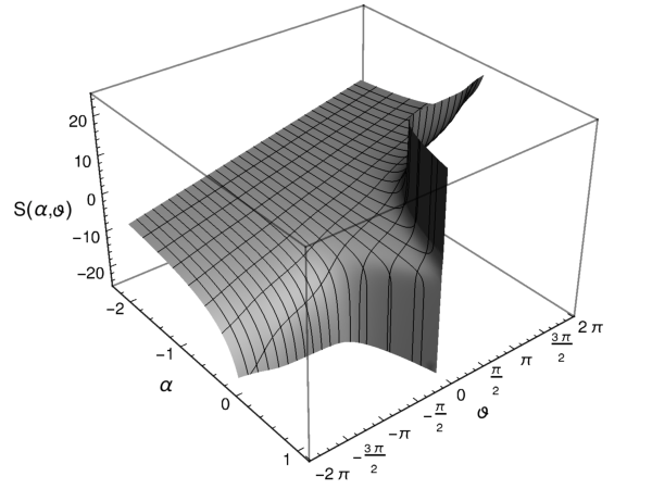
The graph of the function SS described by Lemma 3.8 is shown in Fig. 3.

Refer to caption
Figure 3. The function SS is plotted using formulas (3.30), (3.33), (3.34), and (3.35).

The proof of Lemma 3.8 relies on the next auxiliary statement.

Lemma 3.9.

Let x0,ξ0∈ℝx_{0},\xi_{0}\in{\mathbb{R}}, a,b>0a,b>0, and ff be a real-analytic function on the rectangle

Ra,b​(x0,ξ0)={(x,ξ)∈ℝ2:|x−x0|<a​ and ​|ξ−ξ0|<b}.R_{a,b}(x_{0},\xi_{0})=\{(x,\xi)\in{\mathbb{R}}^{2}:|x-x_{0}|<a\mbox{ and }|\xi-\xi_{0}|<b\}.

Then (x,ξ)→∫ξ0ξf⁡(x,ξ′)​d​ξ′(x,\xi)\to\int_{\xi_{0}}^{\xi}f(x,\xi^{\prime})\,d\xi^{\prime} is a real-analytic function on Ra,b​(x0,ξ0)R_{a,b}(x_{0},\xi_{0}).

Proof.

Since ff is real-analytic on Ra,b​(x0,ξ0)R_{a,b}(x_{0},\xi_{0}), there are an open set O⊂ℂ2O\subset{\mathbb{C}}^{2} and a holomorphic function f~\tilde{f} on OO such that Ra,b​(x0,ξ0)⊂OR_{a,b}(x_{0},\xi_{0})\subset O and ff is the restriction of f~\tilde{f} to Ra,b​(x0,ξ0)R_{a,b}(x_{0},\xi_{0}). Let FF denote the function (x,ξ)→∫ξ0ξf⁡(x,ξ′)​d​ξ′(x,\xi)\to\int_{\xi_{0}}^{\xi}f(x,\xi^{\prime})\,d\xi^{\prime} on Ra,b​(x0,ξ0)R_{a,b}(x_{0},\xi_{0}). Fix 0<a′<a0<a^{\prime}<a and 0<b′<b0<b^{\prime}<b. There exist open subsets O′O^{\prime} and O′′O^{\prime\prime} of ℂ{\mathbb{C}} such that Ra′,b′​(x0,ξ0)⊂O′×O′′⊂OR_{a^{\prime},b^{\prime}}(x_{0},\xi_{0})\subset O^{\prime}\times O^{\prime\prime}\subset O. Moreover, we can assume that O′′O^{\prime\prime} is convex. We define the function F~\tilde{F} on O′×O′′O^{\prime}\times O^{\prime\prime} by the formula

F~​(z,ζ)=∫01(ζ−ξ0)​f~​(z,ξ0+(ζ−ξ0)​t)​𝑑t,z∈O′,ζ∈O′′.\tilde{F}(z,\zeta)=\int_{0}^{1}(\zeta-\xi_{0})\tilde{f}(z,\xi_{0}+(\zeta-\xi_{0})t)\,dt,\quad z\in O^{\prime},\zeta\in O^{\prime\prime}.

Clearly, F~\tilde{F} is holomorphic on O′×O′′O^{\prime}\times O^{\prime\prime} and coincides with FF on Ra′,b′​(x0,ξ0)R_{a^{\prime},b^{\prime}}(x_{0},\xi_{0}). This means that FF is real-analytic on Ra′,b′​(x0,ξ0)R_{a^{\prime},b^{\prime}}(x_{0},\xi_{0}). Since a′a^{\prime} and b′b^{\prime} can be chosen arbitrarily close to aa and bb, we conclude that FF is real-analytic on Ra,b​(x0,ξ0)R_{a,b}(x_{0},\xi_{0}). ∎

Proof of Lemma 3.8.

We define the function SS on WW by the formula

(3.36) S⁡(α,ϑ)=π​Sinc⁡(π2​α)​∫0ϑd​ϑ′Cos2⁡(π2​α/4)−sin2⁡ϑ′,(α,ϑ)∈W.S(\alpha,\vartheta)=\pi\Sinc(\pi^{2}\alpha)\int_{0}^{\vartheta}\frac{d\vartheta^{\prime}}{\Cos^{2}(\pi^{2}\alpha/4)-\sin^{2}\vartheta^{\prime}},\quad(\alpha,\vartheta)\in W.

Since S0​(α,0)=0S_{0}(\alpha,0)=0 for all 0<α<10<\alpha<1 by (3.30), it follows from (3.32) and (3.36) that S0=S|W0S_{0}=S|_{W_{0}}. For every (α,ϑ)∈W(\alpha,\vartheta)\in W, there is ε>0\varepsilon>0 such that WW contains the rectangle

{(α′,ϑ′)∈ℝ2:|α′−α|<ε​ and ​|ϑ′|<|ϑ|+ε}.\{(\alpha^{\prime},\vartheta^{\prime})\in{\mathbb{R}}^{2}:|\alpha^{\prime}-\alpha|<\varepsilon\mbox{ and }|\vartheta^{\prime}|<|\vartheta|+\varepsilon\}.

It therefore follows from Lemma 3.9 and (3.36) that SS is real-analytic in a neighborhood of every point of WW. This means that SS is real-analytic on WW. Given α<0\alpha<0 and −π/2<ϑ<π/2-\pi/2<\vartheta<\pi/2, we let A⁡(α,ϑ)A(\alpha,\vartheta) denote the right-hand side of (3.34) and set σα=|α|\sigma_{\alpha}=\sqrt{|\alpha|}. Using (1.32), we find for every α<0\alpha<0 that

∂ϑA⁡(α,ϑ)=sh⁡(π​σα)σα​(ch2⁡(π​σα/2)−sin2⁡ϑ)=π​Sinc⁡(π2​α)Cos2⁡(π2​α/4)−sin2⁡ϑ,|ϑ|<π/2.\partial_{\vartheta}A(\alpha,\vartheta)=\frac{\sh(\pi\sigma_{\alpha})}{\sigma_{\alpha}(\ch^{2}(\pi\sigma_{\alpha}/2)-\sin^{2}\vartheta)}=\frac{\pi\Sinc(\pi^{2}\alpha)}{\Cos^{2}(\pi^{2}\alpha/4)-\sin^{2}\vartheta},\quad|\vartheta|<\pi/2.

In view of (3.36) and the equality A⁡(α,0)=0A(\alpha,0)=0, this implies that S⁡(α,ϑ)=A⁡(α,ϑ)S(\alpha,\vartheta)=A(\alpha,\vartheta) for all α<0\alpha<0 and −π/2<ϑ<π/2-\pi/2<\vartheta<\pi/2, i.e., (3.34) holds. Formula (3.33) follows immediately from (3.36) for α=0\alpha=0. Since ϑ→(Cos2⁡(π2​α/4)−sin2⁡ϑ)−1\vartheta\to(\Cos^{2}(\pi^{2}\alpha/4)-\sin^{2}\vartheta)^{-1} is a continuous π\pi-periodic function on ℝ{\mathbb{R}} for every α<0\alpha<0, it follows from (3.36) that

(3.37) S(α,ϑ+π)=S(α,ϑ)+πSinc(π2α)∫−π/2π/2d​ϑ′Cos2⁡(π2​α/4)−sin2⁡ϑ′==S(α,ϑ)+S(α,π/2)−S(α,−π/2)S(\alpha,\vartheta+\pi)=S(\alpha,\vartheta)+\pi\Sinc(\pi^{2}\alpha)\int_{-\pi/2}^{\pi/2}\frac{d\vartheta^{\prime}}{\Cos^{2}(\pi^{2}\alpha/4)-\sin^{2}\vartheta^{\prime}}=\\ =S(\alpha,\vartheta)+S(\alpha,\pi/2)-S(\alpha,-\pi/2)

for all α<0\alpha<0 and ϑ∈ℝ\vartheta\in{\mathbb{R}}. This implies (3.35) because S(α,±π/2)=±π/|α|S(\alpha,\pm\pi/2)=\pm\pi/\sqrt{|\alpha|} by (3.34) and the continuity of SS. The uniqueness of SS follows from the uniqueness theorem for holomorphic functions. ∎

Theorem 3.10.

Let the function SS on WW be as in Lemma 3.8. For every α<1\alpha<1 and ϑ∈ℝ\vartheta\in{\mathbb{R}}, Nα,ϑN_{\alpha,\vartheta} is equal to the set

(3.38) {s∈ℝ:s=S⁡(α,ϑ+π​k)​ for some ​k∈ℤ​ such that ​(α,ϑ+π​k)∈W}.\{s\in{\mathbb{R}}:s=S(\alpha,\vartheta+\pi k)\mbox{ for some }k\in{\mathbb{Z}}\mbox{ such that }(\alpha,\vartheta+\pi k)\in W\}.
Proof.

Given α<1\alpha<1 and ϑ∈ℝ\vartheta\in{\mathbb{R}}, we let N~α,ϑ\tilde{N}_{\alpha,\vartheta} denote the set (3.38). We have to prove that

(3.39) Nα,ϑ=N~α,ϑN_{\alpha,\vartheta}=\tilde{N}_{\alpha,\vartheta}

for all α<1\alpha<1 and ϑ∈ℝ\vartheta\in{\mathbb{R}}. By (3.26) and (3.31), the set Σα,ϑ\Sigma_{\alpha,\vartheta} contains −eS0​(α,ϑ)-e^{S_{0}(\alpha,\vartheta)} for every (α,ϑ)∈W0(\alpha,\vartheta)\in W_{0}. Since SS coincides with S0S_{0} on W0W_{0}, it follows from (3.8) that

(3.40) R⁡(α,ϑ,−eS⁡(α,ϑ))=0R(\alpha,\vartheta,-e^{S(\alpha,\vartheta)})=0

for all (α,ϑ)∈W0(\alpha,\vartheta)\in W_{0}. By Lemma 3.8, the left-hand side of (3.40) is a real-analytic function of (α,ϑ)(\alpha,\vartheta) on WW. In view of the uniqueness theorem for holomorphic functions, this implies that (3.40) remains valid for all (α,ϑ)∈W(\alpha,\vartheta)\in W. Let α<1\alpha<1, ϑ∈ℝ\vartheta\in{\mathbb{R}}, and s∈N~α,ϑs\in\tilde{N}_{\alpha,\vartheta}. Then there is k∈ℤk\in{\mathbb{Z}} such that (α,ϑ+π​k)∈W(\alpha,\vartheta+\pi k)\in W and s=S⁡(α,ϑ+π​k)s=S(\alpha,\vartheta+\pi k). By (3.40), we have R⁡(α,ϑ+π​k,−es)=0R(\alpha,\vartheta+\pi k,-e^{s})=0. By (2.19), it follows that R⁡(α,ϑ,−es)=0R(\alpha,\vartheta,-e^{s})=0, i.e., s∈Nα,ϑs\in N_{\alpha,\vartheta}. We therefore have the inclusion

(3.41) N~α,ϑ⊂Nα,ϑ,α<1,ϑ∈ℝ.\tilde{N}_{\alpha,\vartheta}\subset N_{\alpha,\vartheta},\quad\alpha<1,\,\vartheta\in{\mathbb{R}}.

If (α,ϑ)∈Q0(\alpha,\vartheta)\in Q_{0}, then Nα,ϑ=∅N_{\alpha,\vartheta}=\varnothing by Lemma 3.6 and (3.26) and, therefore, (3.41) implies (3.39). By (3.4), it remains to prove (3.39) for (α,ϑ)∈Q≥1(\alpha,\vartheta)\in Q_{\geq 1}. In this case, there is at least one k∈ℤk\in{\mathbb{Z}} such that (α,ϑ+π​k)∈W(\alpha,\vartheta+\pi k)\in W. We hence have

(3.42) N~α,ϑ≠∅,(α,ϑ)∈Q≥1.\tilde{N}_{\alpha,\vartheta}\neq\varnothing,\quad(\alpha,\vartheta)\in Q_{\geq 1}.

We now prove (3.39) for (α,ϑ)∈Q≥1(\alpha,\vartheta)\in Q_{\geq 1} by separately considering the cases α>0\alpha>0, α=0\alpha=0, and α<0\alpha<0.

1. Let α>0\alpha>0, κ=α\kappa=\sqrt{\alpha}, and E1,E2∈Σα,ϑE_{1},E_{2}\in\Sigma_{\alpha,\vartheta}. By (3.18), we have cos⁡(ϑ±ϑκ)≠0\cos(\vartheta\pm\vartheta_{\kappa})\neq 0 and it follows from (3.9) that |E1/E2|κ=1|E_{1}/E_{2}|^{\kappa}=1 and, hence, E1=E2E_{1}=E_{2}. This means that Σα,ϑ\Sigma_{\alpha,\vartheta} and, consequently, Nα,ϑN_{\alpha,\vartheta} contain at most one element. In view of (3.41) and (3.42), this implies (3.39).

2. Let α=0\alpha=0 and E1,E2∈Σ0,ϑE_{1},E_{2}\in\Sigma_{0,\vartheta}. By (2.18), we have

−ln⁡|E1,2|​cos⁡ϑ+π​sin⁡ϑ=0.-\ln|E_{1,2}|\cos\vartheta+\pi\sin\vartheta=0.

By (3.7), the condition (0,ϑ)∈Q≥1(0,\vartheta)\in Q_{\geq 1} ensures that cos⁡ϑ≠0\cos\vartheta\neq 0. It follows that ln⁡|E1/E2|=0\ln|E_{1}/E_{2}|=0 and, hence, E1=E2E_{1}=E_{2}. This means that Σ0,ϑ\Sigma_{0,\vartheta} and, consequently, N0,ϑN_{0,\vartheta} contain at most one element. In view of (3.41) and (3.42), this implies (3.39).

3. Let α<0\alpha<0 and s∈Nα,ϑs\in N_{\alpha,\vartheta}. Then we have (α,ϑ)∈W(\alpha,\vartheta)\in W and, hence, s′=S⁡(α,ϑ)s^{\prime}=S(\alpha,\vartheta) is an element of N~α,ϑ\tilde{N}_{\alpha,\vartheta}. Let E=−esE=-e^{s} and E′=−es′E^{\prime}=-e^{s^{\prime}}. Since s′∈Nα,ϑs^{\prime}\in N_{\alpha,\vartheta} by (3.41), we have E,E′∈Σα,ϑE,E^{\prime}\in\Sigma_{\alpha,\vartheta}. Let κ=i​|α|\kappa=i\sqrt{|\alpha|}. By (3.18), we have cos⁡(ϑ±ϑκ)≠0\cos(\vartheta\pm\vartheta_{\kappa})\neq 0 and it follows from (3.9) that |E/E′|κ=1|E/E^{\prime}|^{\kappa}=1. This implies that s=s′+2​π​k/|α|s=s^{\prime}+2\pi k/\sqrt{|\alpha|} for some k∈ℤk\in{\mathbb{Z}}. By Lemma 3.8, we conclude that s=S⁡(α,ϑ+π​k)s=S(\alpha,\vartheta+\pi k) and, therefore, s∈N~α,ϑs\in\tilde{N}_{\alpha,\vartheta}. This means that Nα,ϑ⊂N~α,ϑN_{\alpha,\vartheta}\subset\tilde{N}_{\alpha,\vartheta}, whence (3.39) follows by (3.41). ∎

By (1.23), (1.24), (1.25), (3.28), and Theorem 3.10, the set Nα,ϑN_{\alpha,\vartheta} is empty for (α,ϑ)∈Q0(\alpha,\vartheta)\in Q_{0}, contains precisely one element for (α,ϑ)∈Q1(\alpha,\vartheta)\in Q_{1}, and is countably infinite for (α,ϑ)∈Q∞(\alpha,\vartheta)\in Q_{\infty}. In view of (3.26), the same is true for Σα,ϑ\Sigma_{\alpha,\vartheta} (the emptiness of Σα,ϑ\Sigma_{\alpha,\vartheta} for (α,ϑ)∈Q0(\alpha,\vartheta)\in Q_{0} also follows from Theorem 3.2). Corollary 3.3 therefore implies that hα,ϑh_{\alpha,\vartheta} has no eigenvalues for (α,ϑ)∈Q0(\alpha,\vartheta)\in Q_{0}, has one eigenvalue for (α,ϑ)∈Q1(\alpha,\vartheta)\in Q_{1}, and has infinitely many eigenvalues for (α,ϑ)∈Q∞(\alpha,\vartheta)\in Q_{\infty}, in agreement with what was claimed in Sec. 1.

Refer to caption
Figure 4. Plots (a), (b), (c), and (d) represent the set NϑN_{\vartheta} for ϑ=±π/2\vartheta=\pm\pi/2, −π/3-\pi/3, 00, and π/6\pi/6 respectively. The horizontal and vertical axes correspond to the variables α\alpha and ss.

We now obtain a graphical representation for the sets Nα,ϑN_{\alpha,\vartheta}. Given ϑ∈ℝ\vartheta\in{\mathbb{R}}, we let NϑN_{\vartheta} denote the subset of (α,s)(\alpha,s)-plane whose sections by the lines α=const\alpha=\mathrm{const} are precisely the sets Nα,ϑN_{\alpha,\vartheta},

Nϑ={(α,s)∈ℝ2:α<1​ and ​s∈Nα,ϑ}.N_{\vartheta}=\{(\alpha,s)\in{\mathbb{R}}^{2}:\alpha<1\mbox{ and }s\in N_{\alpha,\vartheta}\}.

Further, for every ϑ∈ℝ\vartheta\in{\mathbb{R}}, we let SϑS_{\vartheta} denote the function α→S⁡(α,ϑ)\alpha\to S(\alpha,\vartheta) defined on the domain DSϑ={α∈ℝ:(α,ϑ)∈W}D_{S_{\vartheta}}=\{\alpha\in{\mathbb{R}}:(\alpha,\vartheta)\in W\} and set

Gϑ=graph of ​Sϑ={(α,s)∈ℝ2:(α,ϑ)∈W​ and ​s=S⁡(α,ϑ)}.G_{\vartheta}=\mbox{graph of }S_{\vartheta}=\{(\alpha,s)\in{\mathbb{R}}^{2}:(\alpha,\vartheta)\in W\mbox{ and }s=S(\alpha,\vartheta)\}.

By Theorem 3.10, we have

(3.43) Nϑ=⋃k∈ℤGϑ+π​k.N_{\vartheta}=\bigcup_{k\in{\mathbb{Z}}}G_{\vartheta+\pi k}.

It follows from (1.24), (1.25), and (3.28) that

DSϑ={(−∞,ω⁡(ϑ)),|ϑ|≤π/2,ℝ−,|ϑ|>π/2,D_{S_{\vartheta}}=\left\{\begin{matrix}(-\infty,\omega(\vartheta)),&|\vartheta|\leq\pi/2,\\ {\mathbb{R}}_{-},&|\vartheta|>\pi/2,\end{matrix}\right.

where ω\omega is given by (1.22). If |ϑ|<π/2|\vartheta|<\pi/2, then it follows from (3.30) and Lemma 3.8 that

(3.44) Sϑ(α)={1α​ln⁡cos⁡(ϑ−π​α/2)cos⁡(ϑ+π​α/2),0<α<ω⁡(ϑ),π​tg⁡ϑ,α=0,2|α|​arctg⁡(tg⁡ϑ​th⁡π​|α|2),α<0.S_{\vartheta}(\alpha)=\left\{\begin{matrix}\frac{1}{\sqrt{\alpha}}\ln\frac{\cos(\vartheta-\pi\sqrt{\alpha}/2)}{\cos(\vartheta+\pi\sqrt{\alpha}/2)},&0<\alpha<\omega(\vartheta),\\ \pi\tg\vartheta,&\alpha=0,\\ \frac{2}{\sqrt{|\alpha|}}\arctg\left(\tg\vartheta\thyp\frac{\pi\sqrt{|\alpha|}}{2}\right),&\alpha<0.\end{matrix}\right.

Since SS is continuous on WW, we can calculate S±π/2(α)S_{\pm\pi/2}(\alpha) for α<0\alpha<0 by passing to the limits ϑ↑π/2\vartheta\uparrow\pi/2 and ϑ↓−π/2\vartheta\downarrow-\pi/2 in Sϑ​(α)S_{\vartheta}(\alpha). In view of (3.34), we obtain

S±π/2(α)=±π|α|,α<0.S_{\pm\pi/2}(\alpha)=\pm\frac{\pi}{\sqrt{|\alpha|}},\quad\alpha<0.

By Lemma 3.8, we have

DSϑ+π​k=ℝ−,\displaystyle D_{S_{\vartheta+\pi k}}={\mathbb{R}}_{-},
(3.45) Sϑ+π​k​(α)=Sϑ​(α)+2​π​k|α|,α<0,\displaystyle S_{\vartheta+\pi k}(\alpha)=S_{\vartheta}(\alpha)+\frac{2\pi k}{\sqrt{|\alpha|}},\quad\alpha<0,

for every ϑ∈[−π/2,π/2]\vartheta\in[-\pi/2,\pi/2] and every nonzero k∈ℤk\in{\mathbb{Z}}. Formulas (3.43), (3.44), and (3.45) allow us to draw the set NϑN_{\vartheta}, for every ϑ∈ℝ\vartheta\in{\mathbb{R}}. In Fig. 4, this set, which represents the α\alpha-dependence of eigenvalues of hα,ϑh_{\alpha,\vartheta} in the logarithmic scale, is shown for ϑ=±π/2\vartheta=\pm\pi/2, −π/3-\pi/3, 00, and π/6\pi/6. For ϑ≠π/2+π​k\vartheta\neq\pi/2+\pi k, where k∈ℤk\in{\mathbb{Z}}, there is precisely one eigenvalue that crosses the line α=0\alpha=0 in an analytic way, while all other eigenvalues die away at zero or minus infinity as α↑0\alpha\uparrow 0. If ϑ=π/2+π​k\vartheta=\pi/2+\pi k for some k∈ℤk\in{\mathbb{Z}}, then there are no eigenvalues for α≥0\alpha\geq 0.

3.3. Continuous part of 𝒱α,ϑ\mathcal{V}_{\alpha,\vartheta}.

We now consider the absolutely continuous part of the spectral measure 𝒱α,ϑ\mathcal{V}_{\alpha,\vartheta}. By Theorem 3.2, its density tα,ϑt_{\alpha,\vartheta} is given by (3.10). Let the function TT on ℂ×ℂ×ℂ3​π/2{\mathbb{C}}\times{\mathbb{C}}\times{\mathbb{C}}_{3\pi/2} be defined by the formula

(3.46) T⁡(α,ϑ,z)=2​R​(α,ϑ,z)​R⁡(α¯,ϑ¯,z)¯,α,ϑ∈ℂ,z∈ℂ3​π/2.T(\alpha,\vartheta,z)=2R(\alpha,\vartheta,z)\overline{R(\bar{\alpha},\bar{\vartheta},z)},\quad\alpha,\vartheta\in{\mathbb{C}},\,z\in{\mathbb{C}}_{3\pi/2}.

Clearly, (α,ϑ)→T⁡(α,ϑ,z)(\alpha,\vartheta)\to T(\alpha,\vartheta,z) is a holomorphic function on ℂ×ℂ{\mathbb{C}}\times{\mathbb{C}} for every z∈ℂ3​π/2z\in{\mathbb{C}}_{3\pi/2}. If α\alpha and ϑ\vartheta are real, then we have

(3.47) T⁡(α,ϑ,z)=2​|R⁡(α,ϑ,z)|2,z∈ℂ3​π/2,T(\alpha,\vartheta,z)=2|R(\alpha,\vartheta,z)|^{2},\quad z\in{\mathbb{C}}_{3\pi/2},

and it follows from (3.10) that

(3.48) tα,ϑ​(E)=T​(α,ϑ,E)−1,E>0,t_{\alpha,\vartheta}(E)=T(\alpha,\vartheta,E)^{-1},\quad E>0,

for every α<1\alpha<1 and ϑ∈ℝ\vartheta\in{\mathbb{R}}. We shall explicitly express TT in terms of the functions Sinc\Sinc and Cos\Cos. In view of (3.48), this will also give us a formula for the density tα,ϑt_{\alpha,\vartheta}.

Refer to caption
Figure 5. Plots (a), (b), (c), and (d) represent the function 𝔱ϑ​(α,s)\mathfrak{t}_{\vartheta}(\alpha,s) for ϑ=±π/2\vartheta=\pm\pi/2, −π/3-\pi/3, 00, and π/6\pi/6 respectively. The horizontal and vertical axes correspond to the variables α\alpha and ss. The value of 𝔱ϑ\mathfrak{t}_{\vartheta} is encoded in the brightness of the plot: brighter regions correspond to greater values of the function.

By (2.17) and (3.46), we have

(3.49) T⁡(κ2,ϑ,E​ei​ϕ)=2κ2​(E−κ​cos2⁡(ϑ−ϑκ)−CLOSEOPEN−2​cos⁡((π−ϕ)​κ)​cos⁡(ϑ−ϑκ)​cos⁡(ϑ+ϑκ)+Eκ​cos2⁡(ϑ+ϑκ))T(\kappa^{2},\vartheta,Ee^{i\phi})=\frac{2}{\kappa^{2}}\left(E^{-\kappa}\cos^{2}(\vartheta-\vartheta_{\kappa})-\right.\\ \left.-2\cos((\pi-\phi)\kappa)\cos(\vartheta-\vartheta_{\kappa})\cos(\vartheta+\vartheta_{\kappa})+E^{\kappa}\cos^{2}(\vartheta+\vartheta_{\kappa})\right)

for all κ∈ℂ∖{0}\kappa\in{\mathbb{C}}\setminus\{0\}, ϑ∈ℂ\vartheta\in{\mathbb{C}}, E>0E>0, and −π/2<ϕ<3π/2-\pi/2<\phi<3\pi/2. In view of the equality

ln⁡E​Sinc⁡(−κ2​ln2​E)=1κ​sh⁡(κ​ln​E)=Eκ−E−κ2​κ,κ∈ℂ∖{0},E>0,\ln E\Sinc\left(-\kappa^{2}\ln^{2}E\right)=\frac{1}{\kappa}\sh(\kappa\ln E)=\frac{E^{\kappa}-E^{-\kappa}}{2\kappa},\quad\kappa\in{\mathbb{C}}\setminus\{0\},\,E>0,

which follows from (1.30), and the trigonometric identities

2​cos2⁡(ϑ±ϑκ)=1+cos⁡2​ϑ​cos⁡π​κ∓sin⁡2​ϑ​sin⁡π​κ,\displaystyle 2\cos^{2}(\vartheta\pm\vartheta_{\kappa})=1+\cos 2\vartheta\cos\pi\kappa\mp\sin 2\vartheta\sin\pi\kappa,
2​cos⁡(ϑ+ϑκ)​cos⁡(ϑ−ϑκ)=cos⁡2​ϑ+cos⁡π​κ,\displaystyle 2\cos(\vartheta+\vartheta_{\kappa})\cos(\vartheta-\vartheta_{\kappa})=\cos 2\vartheta+\cos\pi\kappa,

which hold for all ϑ,κ∈ℂ\vartheta,\kappa\in{\mathbb{C}}, we derive from (3.49) that

(3.50) T⁡(κ2,ϑ,E​ei​ϕ)=ln2⁡E​Sinc2⁡(−κ24​ln2​E)​(1+cos⁡2​ϑ​cos⁡π​κ)−−2​π​ln⁡E​Sinc⁡(−κ2​ln2​E)​sinc​π​κ​sin⁡2​ϑ+2​cos⁡π​κ−cos⁡(π−ϕ)​κκ2​cos⁡2​ϑ++2​1−cos⁡π​κ​cos⁡(π−ϕ)​κκ2T(\kappa^{2},\vartheta,Ee^{i\phi})=\ln^{2}E\Sinc^{2}\left(-\frac{\kappa^{2}}{4}\ln^{2}E\right)(1+\cos 2\vartheta\cos\pi\kappa)-\\ -2\pi\ln E\Sinc\left(-\kappa^{2}\ln^{2}E\right)\sinc\pi\kappa\sin 2\vartheta+2\frac{\cos\pi\kappa-\cos(\pi-\phi)\kappa}{\kappa^{2}}\cos 2\vartheta+\\ +2\frac{1-\cos\pi\kappa\cos(\pi-\phi)\kappa}{\kappa^{2}}

for every κ∈ℂ∖{0}\kappa\in{\mathbb{C}}\setminus\{0\}, ϑ∈ℂ\vartheta\in{\mathbb{C}}, E>0E>0, and −π/2<ϕ<3π/2-\pi/2<\phi<3\pi/2. Let the functions τ\tau and μ\mu on ℂ×ℂ{\mathbb{C}}\times{\mathbb{C}} be defined by the formulas

(3.51) τ⁡(α,ϕ)=(π−ϕ)2​Sinc2⁡((π−ϕ)2​α4)−π2​Sinc2⁡(π2​α4),\displaystyle\tau(\alpha,\phi)=(\pi-\phi)^{2}\Sinc^{2}\left(\frac{(\pi-\phi)^{2}\alpha}{4}\right)-\pi^{2}\Sinc^{2}\left(\frac{\pi^{2}\alpha}{4}\right),
(3.52) μ⁡(α,ϕ)=2​π2​Sinc2⁡(π2​α)+Cos⁡(π2​α)​τ​(α,ϕ)\displaystyle\mu(\alpha,\phi)=2\pi^{2}\Sinc^{2}(\pi^{2}\alpha)+\Cos(\pi^{2}\alpha)\tau(\alpha,\phi)

for every α,ϕ∈ℂ\alpha,\phi\in{\mathbb{C}}. Performing elementary trigonometric transformations, we obtain

(3.53) τ⁡(κ2,ϕ)=4κ2​(sin2⁡(π−ϕ)​κ2−sin2⁡π​κ2)=2​cos⁡π​κ−cos⁡(π−ϕ)​κκ2,\displaystyle\tau(\kappa^{2},\phi)=\frac{4}{\kappa^{2}}\left(\sin^{2}\frac{(\pi-\phi)\kappa}{2}-\sin^{2}\frac{\pi\kappa}{2}\right)=2\frac{\cos\pi\kappa-\cos(\pi-\phi)\kappa}{\kappa^{2}},
(3.54) μ⁡(κ2,ϕ)=2​sin2⁡π​κκ2+τ⁡(κ2,ϕ)​cos⁡π​κ=2​1−cos⁡π​κ​cos⁡(π−ϕ)​κκ2\displaystyle\mu(\kappa^{2},\phi)=2\frac{\sin^{2}\pi\kappa}{\kappa^{2}}+\tau(\kappa^{2},\phi)\cos\pi\kappa=2\frac{1-\cos\pi\kappa\,\cos(\pi-\phi)\kappa}{\kappa^{2}}

for all κ∈ℂ∖{0}\kappa\in{\mathbb{C}}\setminus\{0\} and ϕ∈ℂ\phi\in{\mathbb{C}}. In view of these formulas, (3.50) implies that

(3.55) T⁡(α,ϑ,E​ei​ϕ)=ln2⁡E​Sinc2⁡(−α4​ln2​E)​(1+cos⁡2​ϑ​Cos⁡(π2​α))−−2​π​ln⁡E​Sinc⁡(−α​ln2​E)​Sinc⁡(π2​α)​sin⁡2​ϑ+τ⁡(α,ϕ)​cos⁡2​ϑ+μ⁡(α,ϕ)T(\alpha,\vartheta,Ee^{i\phi})=\ln^{2}E\Sinc^{2}\left(-\frac{\alpha}{4}\ln^{2}E\right)(1+\cos 2\vartheta\Cos(\pi^{2}\alpha))-\\ -2\pi\ln E\Sinc\left(-\alpha\ln^{2}E\right)\Sinc(\pi^{2}\alpha)\sin 2\vartheta+\tau(\alpha,\phi)\cos 2\vartheta+\mu(\alpha,\phi)

for all α∈ℂ∖{0}\alpha\in{\mathbb{C}}\setminus\{0\}, ϑ∈ℂ\vartheta\in{\mathbb{C}}, E>0E>0, and −π/2<ϕ<3π/2-\pi/2<\phi<3\pi/2. By continuity, this equality remains valid for α=0\alpha=0. Thus, (3.55) holds for all α,ϑ∈ℂ\alpha,\vartheta\in{\mathbb{C}}, E>0E>0, and −π/2<ϕ<3π/2-\pi/2<\phi<3\pi/2.

Formulas (3.48) and (3.55) can be illustrated by drawing the graphs of the density tα,ϑ​(E)t_{\alpha,\vartheta}(E) as a function of α\alpha and EE for various values of ϑ\vartheta. For this, it is convenient to use the logarithmic scale for the energy variable and multiply the density tα,ϑt_{\alpha,\vartheta} by the factor μ⁡(α,0)=2​π2​Sinc2⁡(π2​α)\mu(\alpha,0)=2\pi^{2}\Sinc^{2}(\pi^{2}\alpha). More precisely, given ϑ∈ℝ\vartheta\in{\mathbb{R}}, we define the function 𝔱ϑ\mathfrak{t}_{\vartheta} on (−∞,1)×ℝ(-\infty,1)\times{\mathbb{R}} by setting

(3.56) 𝔱ϑ​(α,s)=2​π2​Sinc2⁡(π2​α)​tα,ϑ​(es),s∈ℝ,α<1.\mathfrak{t}_{\vartheta}(\alpha,s)=2\pi^{2}\Sinc^{2}(\pi^{2}\alpha)t_{\alpha,\vartheta}(e^{s}),\quad s\in{\mathbb{R}},\,\alpha<1.

By (3.48), (3.52), and (3.55), we have

(3.57) 𝔱ϑ​(α,s)−1=1+s2Sinc2(−αs2/4)2​π2​Sinc2⁡(π2​α)​(1+cos⁡2​ϑ​Cos⁡(π2​α))−s​Sinc⁡(−α​s2)π​Sinc⁡(π2​α)​sin⁡2​ϑ\mathfrak{t}_{\vartheta}(\alpha,s)^{-1}=1+\frac{s^{2}\Sinc^{2}\left(-\alpha s^{2}/4\right)}{2\pi^{2}\Sinc^{2}(\pi^{2}\alpha)}(1+\cos 2\vartheta\Cos(\pi^{2}\alpha))-\frac{s\Sinc\left(-\alpha s^{2}\right)}{\pi\Sinc(\pi^{2}\alpha)}\sin 2\vartheta

for every α<1\alpha<1 and ϑ,s∈ℝ\vartheta,s\in{\mathbb{R}}. In Fig. 5, the function 𝔱ϑ\mathfrak{t}_{\vartheta} is plotted using this formula for ϑ=±π/2\vartheta=\pm\pi/2, −π/3-\pi/3, 00, and π/6\pi/6.

Refer to caption
Figure 6. The function Jα,ϑ​(s,ϕ)J_{\alpha,\vartheta}(s,\phi) is plotted for α=−1/2\alpha=-1/2 and ϑ=π/6\vartheta=\pi/6. As in Fig. 5, brighter regions correspond to greater values of the function.

The comparison between Figs. 4 and 5 shows that the α\alpha-dependence of eigenvalues and the density of the continuous part of 𝒱α,ϑ\mathcal{V}_{\alpha,\vartheta} follows the same pattern. This phenomenon can be easily understood if we recall that the point and continuous parts of 𝒱α,ϑ\mathcal{V}_{\alpha,\vartheta} are both determined by the imaginary part of ℳα,ϑ\mathscr{M}_{\alpha,\vartheta} via (2.26) and consider its behaviour in the upper complex half-plane. As in the case of the density tα,ϑt_{\alpha,\vartheta}, to facilitate the visualization of Im​ℳα,ϑ​(z)\mathrm{Im}\,\mathscr{M}_{\alpha,\vartheta}(z), we multiply it by 2​π2​Sinc2⁡(π2​α)2\pi^{2}\Sinc^{2}(\pi^{2}\alpha) and pass to the logarithmic scale for |z||z|. Therefore, for every α<1\alpha<1 and ϑ∈ℝ\vartheta\in{\mathbb{R}}, we introduce the function Jα,ϑJ_{\alpha,\vartheta} on ℝ×[0,π){\mathbb{R}}\times[0,\pi) that is defined by the formula

(3.58) Jα,ϑ​(s,ϕ)=2​π2​Sinc2⁡(π2​α)​Im​ℳα,ϑ​(es+i​ϕ)==2π(π−ϕ)Sinc((π−ϕ)2α)Sinc(π2α)T(α,ϑ,es+i​ϕ)−1,s∈ℝ, 0≤ϕ<π,J_{\alpha,\vartheta}(s,\phi)=2\pi^{2}\Sinc^{2}(\pi^{2}\alpha)\,\mathrm{Im}\,\mathscr{M}_{\alpha,\vartheta}(e^{s+i\phi})=\\ =2\pi(\pi-\phi)\Sinc((\pi-\phi)^{2}\alpha)\Sinc(\pi^{2}\alpha)T(\alpha,\vartheta,e^{s+i\phi})^{-1},\quad s\in{\mathbb{R}},\,0\leq\phi<\pi,

where the second equality follows from (2.23), (2.25), and (3.47). In view of (3.48) and (3.56), we have Jα,ϑ​(s,0)=𝔱ϑ​(α,s)J_{\alpha,\vartheta}(s,0)=\mathfrak{t}_{\vartheta}(\alpha,s) for every α<1\alpha<1 and ϑ,s∈ℝ\vartheta,s\in{\mathbb{R}}. Using (3.55), we can explicitly express Jα,ϑJ_{\alpha,\vartheta} in terms of Sinc\Sinc and Cos\Cos. In Fig. 6, the function Jα,ϑJ_{\alpha,\vartheta} is plotted for α=−1/2\alpha=-1/2 and ϑ=π/6\vartheta=\pi/6. We see that the graph of Jα,ϑJ_{\alpha,\vartheta} contains equidistant vertical ridges that connect the points of Nα,ϑN_{\alpha,\vartheta} at their upper ends with the maxima of the function s→𝔱ϑ​(α,s)s\to\mathfrak{t}_{\vartheta}(\alpha,s) at their lower ends. This means that the graph of Im​ℳα,ϑ\mathrm{Im}\,\mathscr{M}_{\alpha,\vartheta} contains ridges along logarithmically equidistant semicircles in the upper half-plane that connect eigenvalues of hα,ϑh_{\alpha,\vartheta} on the negative half-axis with the maxima of the density tα,ϑt_{\alpha,\vartheta} on the positive half-axis. The values α=−1/2\alpha=-1/2 and ϑ=π/6\vartheta=\pi/6 chosen for Fig. 6 play no special role: the functions Jα,ϑJ_{\alpha,\vartheta} and Im​ℳα,ϑ\mathrm{Im}\,\mathscr{M}_{\alpha,\vartheta} behave in the same way for every α<0\alpha<0 and ϑ∈ℝ\vartheta\in{\mathbb{R}}.

4. Self-adjoint extensions

In this section, we recall basic facts concerning self-adjoint extensions of one-dimensional Schrödinger operators and then apply the general theory to proving Theorem 1.1. We refer the reader to [18, 23, 26] for a detailed treatment of one-dimensional Schrödinger operators.

4.1. General theory

As in Sec. 1, let λ+\lambda_{+} be the restriction to ℝ+{\mathbb{R}}_{+} of the Lebesgue measure λ\lambda on ℝ{\mathbb{R}} and 𝒟\mathcal{D} be the space of all complex continuously differentiable functions on ℝ+{\mathbb{R}}_{+} whose derivative is absolutely continuous on ℝ+{\mathbb{R}}_{+}. Let qq be a complex locally integrable function on ℝ+{\mathbb{R}}_{+}. Given z∈ℂz\in{\mathbb{C}}, we let lq,zl_{q,z} denote the linear operator from 𝒟\mathcal{D} to the space of complex λ+\lambda_{+}-equivalence classes such that

(4.1) (lq,z​f)​(r)=−f′′​(r)+q⁡(r)​f​(r)−z​f​(r)(l_{q,z}f)(r)=-f^{\prime\prime}(r)+q(r)f(r)-zf(r)

for λ\lambda-a.e. r∈ℝ+r\in{\mathbb{R}}_{+} and set

(4.2) lq=lq,0.l_{q}=l_{q,0}.

For every f∈𝒟f\in\mathcal{D} and z∈ℂz\in{\mathbb{C}}, we have lq,z​f=lq​f−z⁡[f]l_{q,z}f=l_{q}f-z[f], where, as in Sec. 1, [f]=[f]λ+[f]=[f]_{\lambda_{+}} denotes the λ+\lambda_{+}-equivalence class of ff. For every a>0a>0 and all complex numbers zz, ζ1\zeta_{1}, and ζ2\zeta_{2}, there is a unique solution ff of the equation lq,z​f=0l_{q,z}f=0 such that f⁡(a)=ζ1f(a)=\zeta_{1} and f′​(a)=ζ2f^{\prime}(a)=\zeta_{2}. This implies that solutions of lq,z​f=0l_{q,z}f=0 constitute a two-dimensional subspace of 𝒟\mathcal{D}. If f,g∈𝒟f,g\in\mathcal{D} are such that Wr​(f,g)W_{r}(f,g) has a limit as r↓0r\downarrow 0, then we set

(4.3) W↓​(f,g)=limr↓0Wr​(f,g).W^{\downarrow}(f,g)=\lim_{r\downarrow 0}W_{r}(f,g).

Similarly, if f,g∈𝒟f,g\in\mathcal{D} are such that Wr​(f,g)W_{r}(f,g) has a limit as r↑∞r\uparrow\infty, then we set

(4.4) W↑​(f,g)=limr↑∞Wr​(f,g).W^{\uparrow}(f,g)=\lim_{r\uparrow\infty}W_{r}(f,g).

In the rest of this subsection, we assume that qq is real. Let

(4.5) 𝒟q={f∈𝒟:f​ and ​lq​f​ are both square-integrable on ​ℝ+}.\mathcal{D}_{q}=\{f\in\mathcal{D}:f\mbox{ and }l_{q}f\mbox{ are both square-integrable on }{\mathbb{R}}_{+}\}.

A λ+\lambda_{+}-measurable complex function ff is said to be left or right square-integrable on ℝ+{\mathbb{R}}_{+} if respectively ∫0a|f⁡(r)|2​𝑑r<∞\int_{0}^{a}|f(r)|^{2}\,dr<\infty or ∫a∞|f⁡(r)|2​𝑑x<∞\int_{a}^{\infty}|f(r)|^{2}\,dx<\infty for any a>0a>0. The subspace of 𝒟\mathcal{D} consisting of left or right square-integrable on ℝ+{\mathbb{R}}_{+} functions ff such that lq​fl_{q}f is also respectively left or right square-integrable on ℝ+{\mathbb{R}}_{+} is denoted by 𝒟q↓\mathcal{D}_{q}^{\downarrow} or 𝒟q↑\mathcal{D}_{q}^{\uparrow}. We obviously have 𝒟q=𝒟q↓∩𝒟q↑\mathcal{D}_{q}=\mathcal{D}_{q}^{\downarrow}\cap\mathcal{D}_{q}^{\uparrow}. It follows from (4.1) by integrating by parts that

∫ab((lq,z​f)​(r)​g​(r)−f⁡(r)​(lq,z​g)​(r))​𝑑r=Wb​(f,g)−Wa​(f,g)\int_{a}^{b}((l_{q,z}f)(r)g(r)-f(r)(l_{q,z}g)(r))\,dr=W_{b}(f,g)-W_{a}(f,g)

for every f,g∈𝒟f,g\in\mathcal{D}, z∈ℂz\in{\mathbb{C}}, and a,b>0a,b>0. This implies the existence of limits in the right-hand sides of (4.3) and (4.4) respectively for every f,g∈𝒟q↓f,g\in\mathcal{D}_{q}^{\downarrow} and f,g∈𝒟q↑f,g\in\mathcal{D}_{q}^{\uparrow}. Hence, W↓​(f,g)W^{\downarrow}(f,g) is well-defined for every f,g∈𝒟q↓f,g\in\mathcal{D}_{q}^{\downarrow} and W↑​(f,g)W^{\uparrow}(f,g) is well-defined for every f,g∈𝒟q↑f,g\in\mathcal{D}_{q}^{\uparrow}. Moreover, it follows that

(4.6) ⟨lq​f,[g]⟩−⟨[f],lq​g⟩=W↑​(f¯,g)−W↓​(f¯,g)\langle l_{q}f,[g]\rangle-\langle[f],l_{q}g\rangle=W^{\uparrow}(\bar{f},g)-W^{\downarrow}(\bar{f},g)

for any f,g∈𝒟qf,g\in\mathcal{D}_{q}, where ⟨⋅,⋅⟩\langle\cdot,\cdot\rangle is the scalar product in L2​(ℝ+)L_{2}({\mathbb{R}}_{+}).

For any linear subspace ZZ of 𝒟q\mathcal{D}_{q}, let Lq​(Z)L_{q}(Z) be the linear operator in L2​(ℝ+)L_{2}({\mathbb{R}}_{+}) defined by the relations

(4.7) DLq​(Z)={[f]:f∈Z},Lq(Z)[f]=lqf,f∈Z.\begin{split}&D_{L_{q}(Z)}=\{[f]:f\in Z\},\\ &L_{q}(Z)[f]=l_{q}f,\quad f\in Z.\end{split}

We define the minimal operator LqL_{q} by setting

(4.8) Lq=Lq​(𝒟q0),L_{q}=L_{q}(\mathcal{D}_{q}^{0}),

where

(4.9) 𝒟q0={f∈𝒟q:W↓​(f,g)=W↑​(f,g)=0​ for every ​g∈𝒟q}.\mathcal{D}_{q}^{0}=\{f\in\mathcal{D}_{q}:W^{\downarrow}(f,g)=W^{\uparrow}(f,g)=0\mbox{ for every }g\in\mathcal{D}_{q}\}.

By (4.6), the operator Lq​(Z)L_{q}(Z) is symmetric if and only if W↓​(f¯,g)=W↑​(f¯,g)W^{\downarrow}(\bar{f},g)=W^{\uparrow}(\bar{f},g) for any f,g∈Zf,g\in Z. In particular, LqL_{q} is a symmetric operator. Moreover, LqL_{q} is closed and densely defined, and its adjoint Lq∗L_{q}^{*} is given by

(4.10) Lq∗=Lq​(𝒟q)L_{q}^{*}=L_{q}(\mathcal{D}_{q})

(see Lemma 9.4 in [23]).

If W↓​(f,g)=0W^{\downarrow}(f,g)=0 for any f,g∈𝒟q↓f,g\in\mathcal{D}_{q}^{\downarrow}, then qq is said to be in the limit point case (l.p.c.) on the left. Otherwise qq is said to be in the limit circle case (l.c.c.) on the left. Similarly, qq is said to be in the l.p.c. on the right if W↑​(f,g)=0W^{\uparrow}(f,g)=0 for any f,g∈𝒟q↑f,g\in\mathcal{D}_{q}^{\uparrow} and to be in the l.c.c. on the right otherwise. According to the well-known Weyl alternative (see, e.g., [23], Theorem 9.9), qq is in the l.c.c. on the left if and only if all solutions of lq​f=0l_{q}f=0 are left square-integrable on ℝ+{\mathbb{R}}_{+} (and, hence, belong to 𝒟q↓\mathcal{D}_{q}^{\downarrow}).

If qq is in the l.p.c. both on the left and on the right, then (4.10) implies that Lq∗L_{q}^{*} is symmetric and, therefore, LqL_{q} is self-adjoint.

If qq is in the l.c.c. on the left and in the l.p.c. on the right, then LqL_{q} has deficiency indices (1,1)(1,1) and the self-adjoint extensions of LqL_{q} are precisely the operators (see [26], Theorem 5.8)

(4.11) Lqf=Lq​(Zqf),L_{q}^{f}=L_{q}(Z_{q}^{f}),

where ff is a nontrivial real solution of lq​f=0l_{q}f=0 and the subspace ZqfZ_{q}^{f} of 𝒟q\mathcal{D}_{q} is given by

(4.12) Zqf={g∈𝒟q:W↓​(f,g)=0}.Z_{q}^{f}=\{g\in\mathcal{D}_{q}:W^{\downarrow}(f,g)=0\}.

The operator LqfL_{q}^{f} determines ff uniquely up to a nonzero real coefficient.

If qq is locally square-integrable on ℝ+{\mathbb{R}}_{+}, then formulas (4.8) and (4.9) imply that C0∞​(ℝ+)C_{0}^{\infty}({\mathbb{R}}_{+}) is contained in 𝒟q0\mathcal{D}_{q}^{0} and LqL_{q} is an extension of Lq​(C0∞​(ℝ+))L_{q}(C_{0}^{\infty}({\mathbb{R}}_{+})).

Lemma 4.1.

Let qq be a real locally square-integrable function on ℝ+{\mathbb{R}}_{+}. Then LqL_{q} is the closure of Lq​(C0∞​(ℝ+))L_{q}(C_{0}^{\infty}({\mathbb{R}}_{+})).

Proof.

See Lemma 17 in [21]. ∎

4.2. The case of the inverse-square potential

By (1.5) and (4.1), we have

(4.13) ℒα,z=lqα,z,α,z∈ℂ,\mathscr{L}_{\alpha,z}=l_{q_{\alpha},z},\quad\alpha,z\in{\mathbb{C}},

where the function qαq_{\alpha} on ℝ+{\mathbb{R}}_{+} is given by (1.4). In view of (1.6) and (4.2), this implies that

(4.14) ℒα=lqα,α∈ℂ.\mathscr{L}_{\alpha}=l_{q_{\alpha}},\quad\alpha\in{\mathbb{C}}.

By (1.15) and (4.13), we obtain

(4.15) lqα,z​𝒰ϑα​(z)=0,α,ϑ,z∈ℂ.l_{q_{\alpha},z}\mathcal{U}^{\alpha}_{\vartheta}(z)=0,\quad\alpha,\vartheta,z\in{\mathbb{C}}.

If α\alpha is real, then qαq_{\alpha} is real. It follows from (1.7), (1.8), (4.5), (4.7), and (4.14) that

(4.16) Δα=𝒟qα,\displaystyle\Delta_{\alpha}=\mathcal{D}_{q_{\alpha}},
(4.17) Hα​(Z)=Lqα​(Z)\displaystyle H_{\alpha}(Z)=L_{q_{\alpha}}(Z)

for every α∈ℝ\alpha\in{\mathbb{R}} and every linear subspace ZZ of Δα\Delta_{\alpha}. Hence, (1.9), (1.10), and Lemma 4.1 imply that

(4.18) hα=Lqα,α∈ℝ.h_{\alpha}=L_{q_{\alpha}},\quad\alpha\in{\mathbb{R}}.

By (4.10), (4.16), (4.17), and (4.18), equality (1.11) holds for all real α\alpha.

If α=κ2\alpha=\kappa^{2} for κ∈ℂ\kappa\in{\mathbb{C}}, then the equation lqα​f=0l_{q_{\alpha}}f=0 has linearly independent solutions r1/2±κr^{1/2\pm\kappa} for κ≠0\kappa\neq 0 and r1/2r^{1/2} and r1/2​ln⁡rr^{1/2}\ln r for κ=0\kappa=0. It follows that

  • (i)

    qαq_{\alpha} is in the l.p.c. both on the left and on the right for α≥1\alpha\geq 1 and

  • (ii)

    qαq_{\alpha} is in the l.p.c. on the right and in the l.c.c. on the left for α<1\alpha<1.

In view of (4.2) and (4.15), we have lqα​𝒰ϑα​(0)=0l_{q_{\alpha}}\mathcal{U}^{\alpha}_{\vartheta}(0)=0 for every α,ϑ∈ℂ\alpha,\vartheta\in{\mathbb{C}}. For α<1\alpha<1 and ϑ∈ℝ\vartheta\in{\mathbb{R}}, the function 𝒰ϑα​(0)\mathcal{U}^{\alpha}_{\vartheta}(0) is real and nontrivial, and it follows from (1.17), (4.12), and (4.16) that Zα,ϑ=Zqα𝒰ϑα​(0)Z_{\alpha,\vartheta}=Z_{q_{\alpha}}^{\mathcal{U}^{\alpha}_{\vartheta}(0)}. By (1.16), (4.11), and (4.17), we conclude that

(4.19) hα,ϑ=Lqα𝒰ϑα​(0),α<1,ϑ∈ℝ.h_{\alpha,\vartheta}=L^{\mathcal{U}^{\alpha}_{\vartheta}(0)}_{q_{\alpha}},\quad\alpha<1,\,\vartheta\in{\mathbb{R}}.
Proof of Theorem 1.1.

In view of (4.18) and condition (i), the operator hαh_{\alpha} is self-adjoint for α≥1\alpha\geq 1. Let α<1\alpha<1. By (4.18) and (4.19), hα,ϑh_{\alpha,\vartheta} a self-adjoint extension of hαh_{\alpha} for every ϑ∈ℝ\vartheta\in{\mathbb{R}}. Conversely, let HH be a self-adjoint extension of hαh_{\alpha}. Then H=LqαfH=L^{f}_{q_{\alpha}} for some nontrivial real f∈𝒟f\in\mathcal{D} satisfying lqα​f=0l_{q_{\alpha}}f=0. By (1.12), (4.2), and (4.13), we have lqα​𝒜α​(0)=lqα​ℬα​(0)=0l_{q_{\alpha}}\mathcal{A}^{\alpha}(0)=l_{q_{\alpha}}\mathcal{B}^{\alpha}(0)=0. Since 𝒜α​(0)\mathcal{A}^{\alpha}(0) and ℬα​(0)\mathcal{B}^{\alpha}(0) are real and linearly independent, it follows from (1.14) that f=c​𝒰ϑα​(0)f=c\,\mathcal{U}^{\alpha}_{\vartheta}(0) for some c,ϑ∈ℝc,\vartheta\in{\mathbb{R}} such that c≠0c\neq 0. In view of (4.19), this means that H=hα,ϑH=h_{\alpha,\vartheta}.

Suppose now that ϑ,ϑ′∈ℝ\vartheta,\vartheta^{\prime}\in{\mathbb{R}} and hα,ϑ=hα,ϑ′h_{\alpha,\vartheta}=h_{\alpha,\vartheta^{\prime}}. By (4.19), we have 𝒰ϑα​(0)=c​𝒰ϑ′α​(0)\mathcal{U}^{\alpha}_{\vartheta}(0)=c\,\mathcal{U}^{\alpha}_{\vartheta^{\prime}}(0) for some nonzero real cc. In view of (1.14), this implies that sinϑ=csinϑ′\sin\vartheta=c\sin\vartheta^{\prime} and cosϑ=ccosϑ′\cos\vartheta=c\cos\vartheta^{\prime} and, therefore, ei​ϑ=c​ei​ϑ′e^{i\vartheta}=ce^{i\vartheta^{\prime}}. It follows that ei⁡(ϑ−ϑ′)=ce^{i(\vartheta-\vartheta^{\prime})}=c, whence c=±1c=\pm 1 and ϑ−ϑ′∈π​ℤ\vartheta-\vartheta^{\prime}\in\pi{\mathbb{Z}}. ∎

5. Eigenfunction expansions

This section consists of two subsections. In the first one, we briefly describe the construction of eigenfunction expansions of one-dimensional Schrödinger operators developed in [10, 16]. This construction, which is adapted to the case of operators with a simple spectrum and relies on so-called singular Titchmarsh–Weyl mm-functions, can be viewed as a variant of Kodaira’s general approach [15] based on matrix-valued measures (see Remark 16 in [21]). In the second subsection, we prove Theorem 1.2 by applying the general theory to the case of the inverse-square potential.

5.1. General theory

Let qq be a real locally integrable function on ℝ+{\mathbb{R}}_{+}. We assume that qq is in the l.c.c. on the left and in the l.p.c. on the right.

Let O⊂ℂO\subset{\mathbb{C}} be an open set. We say that a map u:O→𝒟u\colon O\to\mathcal{D} is a qq-solution on OO if lq,z​u​(z)=0l_{q,z}u(z)=0 for every z∈Oz\in O. A qq-solution uu on OO is said to be holomorphic if the functions z→u⁡(z|r)z\to u(z|r) and z→∂ru⁡(z|r)z\to\partial_{r}u(z|r) are holomorphic on OO for any r∈ℝ+r\in{\mathbb{R}}_{+}. A qq-solution uu on OO is said to be nonvanishing if u⁡(z)≠0u(z)\neq 0 for every z∈Oz\in O. A qq-solution in ℂ{\mathbb{C}} is said to be real-entire if it is holomorphic on ℂ{\mathbb{C}} and u⁡(E)u(E) is real for every E∈ℝE\in{\mathbb{R}}.

Let uu be a real-entire qq-solution. Since qq is in l.c.c. on the left, we have u⁡(z)∈𝒟q↓u(z)\in\mathcal{D}_{q}^{\downarrow} for every z∈ℂz\in{\mathbb{C}}. Suppose that uu is nonvanishing and

(5.1) W↓​(u⁡(z),u⁡(z′))=0,z,z′∈ℂ.W^{\downarrow}(u(z),u(z^{\prime}))=0,\quad z,z^{\prime}\in{\mathbb{C}}.

Let vv be a nonvanishing holomorphic qq-solution on ℂ+{\mathbb{C}}_{+} such that v⁡(z)v(z) is right square-integrable for every z∈ℂ+z\in{\mathbb{C}}_{+} (such a vv always exists; see Lemma 9.8 in [23]). If W⁡(u⁡(z),v⁡(z))=0W(u(z),v(z))=0 for some z∈ℂ+z\in{\mathbb{C}}_{+},1010 10 We recall that W⁡(f,g)W(f,g) denotes the value of the function r→Wr​(f,g)r\to W_{r}(f,g) if f,g∈𝒟f,g\in\mathcal{D} are such that this function is constant (in particular, if lq,z​f=lq,z​g=0l_{q,z}f=l_{q,z}g=0 for some z∈ℂz\in{\mathbb{C}}). then u⁡(z)u(z) is proportional to v⁡(z)v(z) and, hence, u⁡(z)∈𝒟qu(z)\in\mathcal{D}_{q}. In view of (4.12) and (5.1), this means that u⁡(z)∈Zqu⁡(0)u(z)\in Z_{q}^{u(0)} and, therefore, [u⁡(z)][u(z)] is an eigenvector of the self-adjoint operator Lqu⁡(0)L_{q}^{u(0)} with the eigenvalue zz. But this cannot be the case because all eigenvalues of Lqu⁡(0)L_{q}^{u(0)} must be real. It follows that W⁡(u⁡(z),v⁡(z))≠0W(u(z),v(z))\neq 0 for all z∈ℂ+z\in{\mathbb{C}}_{+}.

Given a nonvanishing real-entire qq-solution uu, one can always find another real-entire qq-solution u~\tilde{u} such that W​(u​(z),u~​(z))≠0W(u(z),\tilde{u}(z))\neq 0 for all z∈ℂz\in{\mathbb{C}} (see Lemma 2.4 in [16]).

Let uu and u~\tilde{u} be real-entire qq-solutions such that (5.1) holds and W​(u​(z),u~​(z))≠0W(u(z),\tilde{u}(z))\neq 0 for all z∈ℂz\in{\mathbb{C}}. We define the holomorphic function ℳu,u~q\mathcal{M}^{q}_{u,\tilde{u}} on ℂ+{\mathbb{C}}_{+} by setting

(5.2) ℳu,u~q​(z)=1π​W​(v​(z),u~​(z))W⁡(v⁡(z),u⁡(z))​W​(u⁡(z),u~​(z)),\mathcal{M}^{q}_{u,\tilde{u}}(z)=\frac{1}{\pi}\frac{W(v(z),\tilde{u}(z))}{W(v(z),u(z))W(u(z),\tilde{u}(z))},

where vv is a nonvanishing holomorphic qq-solution on ℂ+{\mathbb{C}}_{+} such that v⁡(z)v(z) is right square-integrable for all z∈ℂ+z\in{\mathbb{C}}_{+} (since qq is in the l.p.c. on the right, this definition is independent of the choice of vv). Following [16], we call such functions singular Titchmarsh-Weyl mm-functions.

The proof of the next statement can be found in [16].

Proposition 5.1.

Let a locally integrable real function qq on ℝ+{\mathbb{R}}_{+} be in the l.c.c. on the left and in the l.p.c. on the right. Let uu be a nonvanishing real-entire qq solution such that (5.1)(\ref{bbb}) holds for all z∈ℂz\in{\mathbb{C}}. Then the following statements hold:

  • 1.1.

    There exists a unique positive Radon measure ν\nu on ℝ{\mathbb{R}} (called the spectral measure for qq and uu) such that

    ∫φ⁡(E)​Im​ℳu,u~q​(E+i​η)​𝑑E→∫φ⁡(E)​𝑑ν​(E)(η↓0)\int\varphi(E)\,\mathrm{Im}\,\mathcal{M}^{q}_{u,\tilde{u}}(E+i\eta)\,dE\to\int\varphi(E)\,d\nu(E)\quad(\eta\downarrow 0)

    for every continuous function φ\varphi on ℝ{\mathbb{R}} with compact support and every real-entire qq-solution u~\tilde{u} such that W​(u​(z),u~​(z))≠0W(u(z),\tilde{u}(z))\neq 0 for every z∈ℂz\in{\mathbb{C}}.

  • 2.2.

    Let ν\nu be the spectral measure for qq and uu. There is a unique unitary operator U:L2​(ℝ+)→L2​(ℝ,ν)U\colon L_{2}({\mathbb{R}}_{+})\to L_{2}({\mathbb{R}},\nu) (called the spectral transformation for qq and uu) such that

    (U​ψ)​(E)=∫ℝ+u⁡(E|r)​ψ​(r)​𝑑r,ψ∈L2c​(ℝ+),(U\psi)(E)=\int_{{\mathbb{R}}_{+}}u(E|r)\psi(r)\,dr,\quad\psi\in L_{2}^{c}({\mathbb{R}}_{+}),

    for ν\nu-a.e. EE.

  • 3.3.

    Let ν\nu and UU be the spectral measure and transformation for qq and uu. Then we have Lqu⁡(0)=U−1​𝒯ιν​UL_{q}^{u(0)}=U^{-1}\mathcal{T}^{\nu}_{\iota}U, where ι\iota is the identity function on ℝ{\mathbb{R}}.

In the next subsection, we shall verify that 𝒱α,ϑ\mathcal{V}_{\alpha,\vartheta} is actually the spectral measure for qαq_{\alpha} and 𝒰ϑα\mathcal{U}^{\alpha}_{\vartheta}. This justifies using the same term “spectral measure” for 𝒱α,ϑ\mathcal{V}_{\alpha,\vartheta} and for the measures described by Proposition 5.1.

5.2. The case of the inverse-square potential

For any κ∈ℂ\kappa\in{\mathbb{C}}, we define the map 𝔳κ:ℂ3​π/2→𝒟\mathfrak{v}^{\kappa}\colon{\mathbb{C}}_{3\pi/2}\to\mathcal{D} by the relation

(5.3) 𝔳κ​(z|r)=i​π2​ei​π​κ/2​r1/2​Hκ(1)​(r​z1/2),r∈ℝ+,z∈ℂ3​π/2,\mathfrak{v}^{\kappa}(z|r)=\frac{i\pi}{2}e^{i\pi\kappa/2}r^{1/2}H^{(1)}_{\kappa}(rz^{1/2}),\quad r\in{\mathbb{R}}_{+},\,z\in{\mathbb{C}}_{3\pi/2},

where Hκ(1)H^{(1)}_{\kappa} is the first Hankel function of order κ\kappa. Because Hκ(1)H^{(1)}_{\kappa} is a solution of the Bessel equation, we have

(5.4) ℒκ2,z​𝔳κ​(z)=0,κ∈ℂ,z∈ℂ3​π/2.\mathscr{L}_{\kappa^{2},z}\mathfrak{v}^{\kappa}(z)=0,\quad\kappa\in{\mathbb{C}},\,z\in{\mathbb{C}}_{3\pi/2}.

It follows from the relation H−κ(1)=ei​π​κ​Hκ(1)H^{(1)}_{-\kappa}=e^{i\pi\kappa}H^{(1)}_{\kappa} (formula (9) in Sec. 7.2.1 in [7]) that

(5.5) 𝔳−κ​(z)=𝔳κ​(z),κ∈ℂ,z∈ℂ3​π/2.\mathfrak{v}^{-\kappa}(z)=\mathfrak{v}^{\kappa}(z),\quad\kappa\in{\mathbb{C}},\,z\in{\mathbb{C}}_{3\pi/2}.

In view of (2.5) and (5.4), the Wronskian Wr​(𝔳κ​(z),𝔲±κ​(z))W_{r}(\mathfrak{v}^{\kappa}(z),\mathfrak{u}^{\pm\kappa}(z)) does not depend on rr. To find it explicitly, we can use the expression for the Wronskian of Bessel functions (formula (29) in Sec. 7.11 in [7]),

(5.6) Wz​(Jκ,Hκ(1))=2​iπ​z.W_{z}(J_{\kappa},H^{(1)}_{\kappa})=\frac{2i}{\pi z}.

Taking (5.5) into account and combining (5.6) with (2.1), (2.3), and (5.3), we derive that

(5.7) W(𝔳κ(z),𝔲κ(z))=z−κ/2ei​π​κ/2,W(𝔳κ(z),𝔲−κ(z))=zκ/2e−iπκ/2W(\mathfrak{v}^{\kappa}(z),\mathfrak{u}^{\kappa}(z))=z^{-\kappa/2}e^{i\pi\kappa/2},\quad W(\mathfrak{v}^{\kappa}(z),\mathfrak{u}^{-\kappa}(z))=z^{\kappa/2}e^{-i\pi\kappa/2}

for any κ∈ℂ\kappa\in{\mathbb{C}} and z∈ℂ3​π/2z\in{\mathbb{C}}_{3\pi/2}.

For α∈ℂ\alpha\in{\mathbb{C}} and z∈ℂ3​π/2z\in{\mathbb{C}}_{3\pi/2}, let the function 𝒱α​(z)\mathscr{V}^{\alpha}(z) on ℝ+{\mathbb{R}}_{+} be defined by the relation 𝒱α​(z)=𝔳κ​(z)\mathscr{V}^{\alpha}(z)=\mathfrak{v}^{\kappa}(z), where κ∈ℂ\kappa\in{\mathbb{C}} is such that κ2=α\kappa^{2}=\alpha (by (5.5), this definition does not depend on the choice of κ\kappa). We therefore have

(5.8) 𝒱κ2​(z)=𝔳κ​(z)\mathscr{V}^{\kappa^{2}}(z)=\mathfrak{v}^{\kappa}(z)

for every κ∈ℂ\kappa\in{\mathbb{C}} and z∈ℂ3​π/2z\in{\mathbb{C}}_{3\pi/2}. By (5.4) and (5.8), we obtain

(5.9) ℒα,z​𝒱α​(z)=0,z∈ℂ3​π/2,α∈ℂ.\mathscr{L}_{\alpha,z}\mathscr{V}^{\alpha}(z)=0,\quad z\in{\mathbb{C}}_{3\pi/2},\,\alpha\in{\mathbb{C}}.

Using the well-known asymptotic form of Hκ(1)​(ζ)H^{(1)}_{\kappa}(\zeta) for ζ→∞\zeta\to\infty (see formula (1) in Sec. 7.13.1 in [7]), we find that

𝔳κ(z|r)∼2−1π(i+1)z−1/4ei​z1/2​r,r→∞,\mathfrak{v}^{\kappa}(z|r)\sim 2^{-1}\sqrt{\pi}(i+1)z^{-1/4}e^{iz^{1/2}r},\quad r\to\infty,

for every κ∈ℂ\kappa\in{\mathbb{C}} and z∈ℂ3​π/2z\in{\mathbb{C}}_{3\pi/2} and, hence, 𝔳κ​(z)\mathfrak{v}^{\kappa}(z) is right square-integrable for all κ∈ℂ\kappa\in{\mathbb{C}} and z∈ℂ+z\in{\mathbb{C}}_{+}. In view of (5.8), this implies that 𝒱α​(z)\mathscr{V}^{\alpha}(z) is right square-integrable for all α∈ℂ\alpha\in{\mathbb{C}} and z∈ℂ+z\in{\mathbb{C}}_{+}.

Lemma 5.2.

There is a unique holomorphic function FF on ℂ×ℂ3​π/2×ℂπ{\mathbb{C}}\times{\mathbb{C}}_{3\pi/2}\times{\mathbb{C}}_{\pi} such that F⁡(α,z,r)=𝒱α​(z|r)F(\alpha,z,r)=\mathscr{V}^{\alpha}(z|r) for every α∈ℂ\alpha\in{\mathbb{C}}, z∈ℂ3​π/2z\in{\mathbb{C}}_{3\pi/2}, and r>0r>0.

Proof.

By (5.3), there is a holomorphic function GG on ℂ×ℂ3​π/2×ℂπ{\mathbb{C}}\times{\mathbb{C}}_{3\pi/2}\times{\mathbb{C}}_{\pi} such that G⁡(κ,z,r)=𝔳κ​(z|r)G(\kappa,z,r)=\mathfrak{v}^{\kappa}(z|r) for every κ∈ℂ\kappa\in{\mathbb{C}}, z∈ℂ3​π/2z\in{\mathbb{C}}_{3\pi/2}, and r>0r>0. It follows from (5.5) and the uniqueness theorem for holomorphic functions that G⁡(κ,z,ζ)=G⁡(−κ,z,ζ)G(\kappa,z,\zeta)=G(-\kappa,z,\zeta) for all κ∈ℂ\kappa\in{\mathbb{C}}, z∈ℂ3​π/2z\in{\mathbb{C}}_{3\pi/2}, and ζ∈ℂπ\zeta\in{\mathbb{C}}_{\pi}. The existence of FF with the required properties is now ensured by Lemma A.3 and (5.8). The uniqueness of FF follows from the uniqueness theorem for holomorphic functions. ∎

It follows immediately from (1.13) that the identity

(5.10) Wr​(f1​f2,f3​f4)=f1​(r)​f3​(r)​Wr​(f2,f4)+Wr​(f1,f3)​f2​(r)​f4​(r)W_{r}(f_{1}f_{2},f_{3}f_{4})=f_{1}(r)f_{3}(r)W_{r}(f_{2},f_{4})+W_{r}(f_{1},f_{3})f_{2}(r)f_{4}(r)

holds for every f1,f2,f3,f4∈𝒟f_{1},f_{2},f_{3},f_{4}\in\mathcal{D} and r>0r>0.

Lemma 5.3.

Let κ∈ℂ\kappa\in{\mathbb{C}} be such that |Re​κ|<1|\mathrm{Re}\,\kappa|<1. Then we have

(5.11) W↓​(𝔲κ​(z),𝔲κ​(z′))=0,W↓​(𝔲κ​(z),𝔲−κ​(z′))=−2π​sin⁡π​κW^{\downarrow}(\mathfrak{u}^{\kappa}(z),\mathfrak{u}^{\kappa}(z^{\prime}))=0,\quad W^{\downarrow}(\mathfrak{u}^{\kappa}(z),\mathfrak{u}^{-\kappa}(z^{\prime}))=-\frac{2}{\pi}\sin\pi\kappa

for every z,z′∈ℂz,z^{\prime}\in{\mathbb{C}}.

Proof.

By (2.1) and (5.10), we have

(5.12) Wr​(𝔲κ​(z),𝔲κ​(z′))=2​r2+2​κ​(z′​𝒳κ​(r2​z)​𝒳κ′​(r2​z′)−z​𝒳κ′​(r2​z)​𝒳κ​(r2​z′)),W_{r}(\mathfrak{u}^{\kappa}(z),\mathfrak{u}^{\kappa}(z^{\prime}))=2r^{2+2\kappa}(z^{\prime}\mathcal{X}_{\kappa}(r^{2}z)\mathcal{X}^{\prime}_{\kappa}(r^{2}z^{\prime})-z\mathcal{X}^{\prime}_{\kappa}(r^{2}z)\mathcal{X}_{\kappa}(r^{2}z^{\prime})),
(5.13) Wr​(𝔲κ​(z),𝔲−κ​(z′))=−2​κ​𝒳κ​(r2​z)​𝒳−κ​(r2​z′)++2​r2​(z′​𝒳κ​(r2​z)​𝒳−κ′​(r2​z′)−z​𝒳κ′​(r2​z)​𝒳−κ​(r2​z′))W_{r}(\mathfrak{u}^{\kappa}(z),\mathfrak{u}^{-\kappa}(z^{\prime}))=-2\kappa\mathcal{X}_{\kappa}(r^{2}z)\mathcal{X}_{-\kappa}(r^{2}z^{\prime})+\\ +2r^{2}(z^{\prime}\mathcal{X}_{\kappa}(r^{2}z)\mathcal{X}^{\prime}_{-\kappa}(r^{2}z^{\prime})-z\mathcal{X}^{\prime}_{\kappa}(r^{2}z)\mathcal{X}_{-\kappa}(r^{2}z^{\prime}))

for all z,z′∈ℂz,z^{\prime}\in{\mathbb{C}} and r>0r>0. Since |Re​κ|<1|\mathrm{Re}\,\kappa|<1, the left equality in (5.11) follows from (5.12) for every z,z′∈ℂz,z^{\prime}\in{\mathbb{C}}. Formula (2.2) implies that

𝒳κ​(0)​𝒳−κ​(0)=(Γ⁡(1+κ)​Γ​(1−κ))−1=sinc⁡π​κ.\mathcal{X}_{\kappa}(0)\mathcal{X}_{-\kappa}(0)=(\Gamma(1+\kappa)\Gamma(1-\kappa))^{-1}=\sinc\pi\kappa.

By (5.13), we conclude that the right equality in (5.11) holds for all z,z′∈ℂz,z^{\prime}\in{\mathbb{C}}. ∎

Lemma 5.4.

Let α<1\alpha<1 and ϑ∈ℝ\vartheta\in{\mathbb{R}}. Then we have

(5.14) W↓​(𝒰ϑα​(z),𝒰ϑα​(z′))=0,z,z′∈ℂ.W^{\downarrow}(\mathcal{U}^{\alpha}_{\vartheta}(z),\mathcal{U}^{\alpha}_{\vartheta}(z^{\prime}))=0,\quad z,z^{\prime}\in{\mathbb{C}}.
Proof.

Let α≠0\alpha\neq 0 and κ∈ℂ\kappa\in{\mathbb{C}} be such that κ2=α\kappa^{2}=\alpha. By (2.14), we have

(5.15) α​Wr​(𝒰ϑα​(z),𝒰ϑα​(z′))=Wr​(uκ​(z),uκ​(z′))​cos2⁡(ϑ−ϑκ)+Wr​(u−κ​(z),u−κ​(z′))​cos2⁡(ϑ+ϑκ)++(Wr​(uκ​(z′),u−κ​(z))−Wr​(uκ​(z),u−κ​(z′)))​cos⁡(ϑ−ϑκ)​cos⁡(ϑ+ϑκ)\alpha W_{r}(\mathcal{U}^{\alpha}_{\vartheta}(z),\mathcal{U}^{\alpha}_{\vartheta}(z^{\prime}))=\\ W_{r}(u^{\kappa}(z),u^{\kappa}(z^{\prime}))\cos^{2}(\vartheta-\vartheta_{\kappa})+W_{r}(u^{-\kappa}(z),u^{-\kappa}(z^{\prime}))\cos^{2}(\vartheta+\vartheta_{\kappa})+\\ +(W_{r}(u^{\kappa}(z^{\prime}),u^{-\kappa}(z))-W_{r}(u^{\kappa}(z),u^{-\kappa}(z^{\prime})))\cos(\vartheta-\vartheta_{\kappa})\cos(\vartheta+\vartheta_{\kappa})

for all z,z′∈ℂz,z^{\prime}\in{\mathbb{C}} and r>0r>0. Since α<1\alpha<1, we have |Re​κ|<1|\mathrm{Re}\,\kappa|<1 and, therefore, (5.14) follows from (5.15) and Lemma 5.3. It remains to consider the case α=0\alpha=0. For every z∈ℂz\in{\mathbb{C}}, we define the smooth functions c⁡(z)c(z) and d⁡(z)d(z) on ℝ{\mathbb{R}} by the relations

c⁡(z|r)=𝒳0​(r2​z),d⁡(z|r)=(γ−ln⁡2)​c​(z|r)−𝒴⁡(r2​z),r∈ℝ.c(z|r)=\mathcal{X}_{0}(r^{2}z),\quad d(z|r)=(\gamma-\ln 2)c(z|r)-\mathcal{Y}(r^{2}z),\quad r\in{\mathbb{R}}.

By (2.1), (2.7), (2.9), and (2.12), we have

𝒜0​(z|r)=2​r1/2​(c⁡(z|r)​ln⁡r+d⁡(z|r)),ℬ0​(z|r)=π​r1/2​c​(z|r),z∈ℂ,r>0.\mathcal{A}^{0}(z|r)=2r^{1/2}(c(z|r)\ln r+d(z|r)),\quad\mathcal{B}^{0}(z|r)=\pi r^{1/2}c(z|r),\quad z\in{\mathbb{C}},\,r>0.

Using (5.10), we obtain

14​Wr​(𝒜0​(z),𝒜0​(z′))=r​ln2​r​Wr​(c⁡(z),c⁡(z′))+r​Wr​(d⁡(z),d⁡(z′))+\displaystyle\frac{1}{4}W_{r}(\mathcal{A}^{0}(z),\mathcal{A}^{0}(z^{\prime}))=r\ln^{2}rW_{r}(c(z),c(z^{\prime}))+rW_{r}(d(z),d(z^{\prime}))+
+r​ln⁡r⁡(Wr​(c⁡(z),d⁡(z′))+Wr​(d⁡(z),c⁡(z′)))+d⁡(z|r)​c​(z′|r)−c⁡(z|r)​d​(z′|r),\displaystyle+r\ln r(W_{r}(c(z),d(z^{\prime}))+W_{r}(d(z),c(z^{\prime})))+d(z|r)c(z^{\prime}|r)-c(z|r)d(z^{\prime}|r),
12​π​Wr​(𝒜0​(z),ℬ0​(z′))=r​Wr​(d⁡(z),c⁡(z′))+r​ln⁡r​Wr​(c⁡(z),c⁡(z′))−c⁡(z|r)​c​(z′|r),\displaystyle\frac{1}{2\pi}W_{r}(\mathcal{A}^{0}(z),\mathcal{B}^{0}(z^{\prime}))=rW_{r}(d(z),c(z^{\prime}))+r\ln rW_{r}(c(z),c(z^{\prime}))-c(z|r)c(z^{\prime}|r),
Wr​(ℬ0​(z),ℬ0​(z′))=π2​r​Wr​(c⁡(z),c⁡(z′))\displaystyle W_{r}(\mathcal{B}^{0}(z),\mathcal{B}^{0}(z^{\prime}))=\pi^{2}rW_{r}(c(z),c(z^{\prime}))

for every r>0r>0 and z,z′∈ℂz,z^{\prime}\in{\mathbb{C}}. Since c⁡(z|0)=1c(z|0)=1 and d⁡(z|0)=γ−ln⁡2d(z|0)=\gamma-\ln 2 for all z∈ℂz\in{\mathbb{C}}, we find that

W↓​(𝒜0​(z),ℬ0​(z′))=−2​π,W↓​(𝒜0​(z),𝒜0​(z′))=W↓​(ℬ0​(z),ℬ0​(z′))=0W^{\downarrow}(\mathcal{A}^{0}(z),\mathcal{B}^{0}(z^{\prime}))=-2\pi,\quad W^{\downarrow}(\mathcal{A}^{0}(z),\mathcal{A}^{0}(z^{\prime}))=W^{\downarrow}(\mathcal{B}^{0}(z),\mathcal{B}^{0}(z^{\prime}))=0

for all z,z′∈ℂz,z^{\prime}\in{\mathbb{C}}. In view of (1.14), this implies (5.14) for α=0\alpha=0. ∎

It follows from (1.15) and (5.9) that Wr​(𝒱α​(z),𝒰ϑα​(z))W_{r}(\mathscr{V}^{\alpha}(z),\mathcal{U}^{\alpha}_{\vartheta}(z)) does not depend on rr for every α,ϑ∈ℂ\alpha,\vartheta\in{\mathbb{C}} and z∈ℂ3​π/2z\in{\mathbb{C}}_{3\pi/2}. It is easy to see that

(5.16) W⁡(𝒱α​(z),𝒰ϑα​(z))=R⁡(α,ϑ,z),α,ϑ∈ℂ,z∈ℂ3​π/2,W(\mathscr{V}^{\alpha}(z),\mathcal{U}^{\alpha}_{\vartheta}(z))=R(\alpha,\vartheta,z),\quad\alpha,\vartheta\in{\mathbb{C}},\,z\in{\mathbb{C}}_{3\pi/2},

where RR is the function defined in Lemma 2.3. Indeed, it follows from (2.14), (5.7), and (5.8) that W⁡(𝒱κ2​(z),𝒰ϑκ2​(z))W(\mathscr{V}^{\kappa^{2}}(z),\mathcal{U}^{\kappa^{2}}_{\vartheta}(z)) is equal to the right-hand side of (2.17) for every κ∈ℂ∖{0}\kappa\in{\mathbb{C}}\setminus\{0\}, ϑ∈ℂ\vartheta\in{\mathbb{C}}, and z∈ℂ3​π/2z\in{\mathbb{C}}_{3\pi/2}. Equality (5.16) therefore holds for all α∈ℂ∖{0}\alpha\in{\mathbb{C}}\setminus\{0\}, ϑ∈ℂ\vartheta\in{\mathbb{C}}, and z∈ℂ3​π/2z\in{\mathbb{C}}_{3\pi/2}. By (1.14) and Lemmas 2.2, 2.3, and 5.2, both sides of (5.16) are holomorphic with respect to (α,ϑ,z)(\alpha,\vartheta,z) on ℂ×ℂ×ℂ3​π/2{\mathbb{C}}\times{\mathbb{C}}\times{\mathbb{C}}_{3\pi/2}. Hence, (5.16) remains valid for α=0\alpha=0.

By (1.14) and (2.16), we have

(5.17) W⁡(𝒰ϑα​(z),𝒰ϑ+π/2α​(z))=−2​π​Sinc2⁡(π2​α),α,ϑ,z∈ℂ.W(\mathcal{U}^{\alpha}_{\vartheta}(z),\mathcal{U}^{\alpha}_{\vartheta+\pi/2}(z))=-2\pi\Sinc^{2}(\pi^{2}\alpha),\quad\alpha,\vartheta,z\in{\mathbb{C}}.
Proof of Theorem 1.2.

It follows immediately from (1.14) and the definition of 𝒜α​(z)\mathcal{A}^{\alpha}(z) and ℬα​(z)\mathcal{B}^{\alpha}(z) that the functions z→𝒰ϑα​(z|r)z\to\mathcal{U}^{\alpha}_{\vartheta}(z|r) and z→∂r𝒰ϑα​(z|r)z\to\partial_{r}\mathcal{U}^{\alpha}_{\vartheta}(z|r) are holomorphic on ℂ{\mathbb{C}} for every r>0r>0 and α,ϑ∈ℂ\alpha,\vartheta\in{\mathbb{C}}. Equality (4.15) therefore implies that 𝒰ϑα\mathcal{U}^{\alpha}_{\vartheta} is a holomorphic qαq_{\alpha}-solution on ℂ{\mathbb{C}} for every α,ϑ∈ℂ\alpha,\vartheta\in{\mathbb{C}}. If α\alpha and ϑ\vartheta are real, then 𝒰ϑα​(E)\mathcal{U}^{\alpha}_{\vartheta}(E) is real for real EE and, hence, 𝒰ϑα\mathcal{U}^{\alpha}_{\vartheta} is a real-entire qαq_{\alpha}-solution. By (5.3) and (5.8), the functions z→𝒱α​(z|r)z\to\mathscr{V}^{\alpha}(z|r) and z→∂r𝒱α​(z|r)z\to\partial_{r}\mathscr{V}^{\alpha}(z|r) are holomorphic on ℂ3​π/2{\mathbb{C}}_{3\pi/2} for every r>0r>0 and α∈ℂ\alpha\in{\mathbb{C}}. In view of (4.13) and (5.9), it follows that 𝒱α\mathscr{V}^{\alpha} is a holomorphic qαq_{\alpha}-solution on ℂ3​π/2{\mathbb{C}}_{3\pi/2} for every α∈ℂ\alpha\in{\mathbb{C}}. Moreover, 𝒱α\mathscr{V}^{\alpha} is nonvanishing for every α∈ℂ\alpha\in{\mathbb{C}} by (5.7) and (5.8).

We now fix α<1\alpha<1 and ϑ∈ℝ\vartheta\in{\mathbb{R}}, set q=qαq=q_{\alpha}, and let uu and u~\tilde{u} denote the real-entire qq-solutions 𝒰ϑα\mathcal{U}^{\alpha}_{\vartheta} and 𝒰ϑ+π/2α\mathcal{U}^{\alpha}_{\vartheta+\pi/2} respectively. Because α<1\alpha<1, (5.17) implies that

(5.18) W⁡(u⁡(z),u~​(z))≠0,z∈ℂ,W(u(z),\tilde{u}(z))\neq 0,\quad z\in{\mathbb{C}},

and, hence, uu is nonvanishing. By Lemma 5.4, we conclude that qq and uu satisfy all conditions of Proposition 5.1. Moreover, it follows from (5.18) that there exists a well-defined Titchmarsh–Weyl mm-function ℳu,u~q\mathcal{M}^{q}_{u,\tilde{u}}. Since 𝒱α​(z)\mathscr{V}^{\alpha}(z) is right square-integrable for every z∈ℂ+z\in{\mathbb{C}}_{+}, the latter can be found by substituting v=𝒱α|ℂ+v=\mathscr{V}^{\alpha}|_{{\mathbb{C}}_{+}} in the right-hand side of (5.2). Using (2.24), (5.16), and (5.17), we obtain ℳu,u~q​(z)=ℳα,ϑ​(z)\mathcal{M}^{q}_{u,\tilde{u}}(z)=\mathscr{M}_{\alpha,\vartheta}(z) for every z∈ℂ+z\in{\mathbb{C}}_{+}. In view of (5.18), statement 1 of Proposition 5.1 and formula (2.26) imply that 𝒱α,ϑ\mathcal{V}_{\alpha,\vartheta} is precisely the spectral measure for qq and uu. The existence and uniqueness of Uα,ϑU_{\alpha,\vartheta} and equality (1.20) are therefore ensured by statements 2 and 3 of Proposition 5.1 and formula (4.19). ∎

6. Smoothness properties of the spectral measure

In this section, we shall establish Theorem 1.3.

Before passing to the proof, we note that the smoothness of 𝒱α,ϑ\mathcal{V}_{\alpha,\vartheta} with respect to α\alpha and ϑ\vartheta is suggested by explicit formulas obtained in Sec. 3. For example, let us set ϑ=π/2\vartheta=\pi/2 and examine the α\alpha-dependence of the point part 𝒱α,π/2p\mathcal{V}^{p}_{\alpha,\pi/2} of the measure 𝒱α,π/2\mathcal{V}_{\alpha,\pi/2}. It follows from (3.26), (3.28), Lemma 3.8, and Theorem 3.10 that Σα,π/2=∅\Sigma_{\alpha,\pi/2}=\varnothing for α≥0\alpha\geq 0 and

Σα,π/2={E∈ℝ:E=−exp((2k+1)π|α|−1/2) for some k∈ℤ}\Sigma_{\alpha,\pi/2}=\left\{E\in{\mathbb{R}}:E=-\exp\left((2k+1)\pi|\alpha|^{-1/2}\right)\mbox{ for some }k\in{\mathbb{Z}}\right\}

for α<0\alpha<0. Let φ∈𝒮\varphi\in\mathscr{S}. In view of (3.12) and (B.2), Theorem 3.2 implies that

(6.1) ∫φ⁡(E)​d​𝒱α,π/2p​(E)=2π2​Sinc⁡(π2​α)​Sinc2⁡(π2​α/4)​∑k∈ℤφ(2​k+1)​π​(α)\int\varphi(E)\,d\mathcal{V}^{p}_{\alpha,\pi/2}(E)=\frac{2}{\pi^{2}\Sinc(\pi^{2}\alpha)\Sinc^{2}(\pi^{2}\alpha/4)}\sum_{k\in{\mathbb{Z}}}\varphi_{(2k+1)\pi}(\alpha)

for every α<1\alpha<1, where φc\varphi_{c}, c∈ℝc\in{\mathbb{R}}, denotes the function on ℝ{\mathbb{R}} that is identically zero on [0,∞)[0,\infty) and is given by

φc(α)=1|α|exp(c|α|−1/2)φ(−exp(c|α|−1/2))\varphi_{c}(\alpha)=\frac{1}{|\alpha|}\exp\left(c|\alpha|^{-1/2}\right)\varphi\left(-\exp\left(c|\alpha|^{-1/2}\right)\right)

for α<0\alpha<0. It follows immediately from the definition of the space 𝒮\mathscr{S} that φc\varphi_{c} is an infinitely differentiable function on ℝ{\mathbb{R}} for every nonzero real cc (however, in general, φc\varphi_{c} is not real-analytic at α=0\alpha=0 even for real-analytic φ\varphi). It is also possible to verify directly that ∑k∈ℤφ(2​k+1)​π\sum_{k\in{\mathbb{Z}}}\varphi_{(2k+1)\pi} is infinitely differentiable on ℝ{\mathbb{R}} and, therefore, the left-hand side of (6.1) is infinitely differentiable with respect to α\alpha on (−∞,1)(-\infty,1).

It seems, however, that a complete proof of Theorem 1.3 (including the continuous part of 𝒱α,ϑ\mathcal{V}_{\alpha,\vartheta} and the dependence on both α\alpha and ϑ\vartheta) based on explicit formulas for the spectral measures would be extremely cumbersome. We shall adopt a different approach based on representation (2.26) of 𝒱α,ϑ\mathcal{V}_{\alpha,\vartheta} as a boundary value of the holomorphic function ℳα,ϑ\mathscr{M}_{\alpha,\vartheta}. The idea is to derive the infinite differentiability of 𝒱α,ϑ\mathcal{V}_{\alpha,\vartheta} with respect to α\alpha and ϑ\vartheta from that of ℳα,ϑ\mathscr{M}_{\alpha,\vartheta}. Lemma 6.1 below gives a condition under which the differentiability of a holomorphic function on ℂ+{\mathbb{C}}_{+} with respect to some parameters implies the same property for its boundary value. This condition involves certain uniform estimates on the derivatives of this function with respect to the parameters in question. In the case of the function ℳα,ϑ\mathscr{M}_{\alpha,\vartheta}, estimates of this type, which are the most nontrivial part of the proof of Theorem 1.3, are provided by Proposition 6.2 below. Combining Lemma 6.1 and Proposition 6.2, we shall obtain the infinite differentiability of 𝒱α,ϑ\mathcal{V}_{\alpha,\vartheta}.

We now give a formal exposition.

For every ϱ,σ≥0\varrho,\sigma\geq 0, we let ℋϱ,σ\mathcal{H}_{\varrho,\sigma} denote the Banach space consisting of all holomorphic functions on ℂ+{\mathbb{C}}_{+} with the finite norm

‖f‖ϱ,σ=supz∈ℂ+|f⁡(z)|​𝒩ϱ,σ​(z),\|f\|_{\varrho,\sigma}=\sup_{z\in{\mathbb{C}}_{+}}|f(z)|\mathcal{N}_{\varrho,\sigma}(z),

where the function 𝒩ϱ,σ\mathcal{N}_{\varrho,\sigma} on ℂ+{\mathbb{C}}_{+} is given by

𝒩ϱ,σ​(z)=1(1+|z|)ϱ​(Im​z1+|z|)σ.\mathcal{N}_{\varrho,\sigma}(z)=\frac{1}{(1+|z|)^{\varrho}}\left(\frac{\mathrm{Im}\,z}{1+|z|}\right)^{\sigma}.

If ϱ′≥ϱ≥0\varrho^{\prime}\geq\varrho\geq 0 and σ′≥σ≥0\sigma^{\prime}\geq\sigma\geq 0, then ℋϱ,σ⊂ℋϱ′,σ′\mathcal{H}_{\varrho,\sigma}\subset\mathcal{H}_{\varrho^{\prime},\sigma^{\prime}} and the inclusion map is continuous. We define the linear space ℋ\mathcal{H} by setting ℋ=⋃ϱ,σ≥0ℋϱ,σ\mathcal{H}=\bigcup_{\varrho,\sigma\geq 0}\mathcal{H}_{\varrho,\sigma}. It is well known (see, e.g., [25], Ch. 5, Sec. 26.3) that ∫ℝf⁡(E+i​η)​φ​(E)​𝑑E\int_{{\mathbb{R}}}f(E+i\eta)\varphi(E)\,dE has a limit as η↓0\eta\downarrow 0 for every f∈ℋf\in\mathcal{H} and φ∈𝒮\varphi\in\mathscr{S}. Given φ∈𝒮\varphi\in\mathscr{S}, we let BφB_{\varphi} denote the map f→limη↓0∫ℝf⁡(E+i​η)​φ​(E)​𝑑Ef\to\lim_{\eta\downarrow 0}\int_{{\mathbb{R}}}f(E+i\eta)\varphi(E)\,dE on ℋ\mathcal{H}. The definitions of 𝒮\mathscr{S} and ℋϱ,σ\mathcal{H}_{\varrho,\sigma} imply that f→∫ℝf⁡(E+i​η)​φ​(E)​𝑑Ef\to\int_{{\mathbb{R}}}f(E+i\eta)\varphi(E)\,dE is a continuous linear functional on ℋϱ,σ\mathcal{H}_{\varrho,\sigma} for every η>0\eta>0, φ∈𝒮\varphi\in\mathscr{S}, and ϱ,σ≥0\varrho,\sigma\geq 0. By the Banach-Steinhaus theorem (see Theorem III.9 in [19]), it follows that the restriction of BφB_{\varphi} to ℋϱ,σ\mathcal{H}_{\varrho,\sigma} is a continuous linear functional on ℋϱ,σ\mathcal{H}_{\varrho,\sigma} for every φ∈𝒮\varphi\in\mathscr{S} and ϱ,σ≥0\varrho,\sigma\geq 0.

Lemma 6.1.

Let ϱ,σ≥0\varrho,\sigma\geq 0, n=1,2,…n=1,2,\ldots, and φ∈𝒮\varphi\in\mathscr{S}. Let OO be an open subset of ℝn{\mathbb{R}}^{n} and MM be a map from OO to ℋϱ,σ\mathcal{H}_{\varrho,\sigma} such that x→M⁡(x|z)x\to M(x|z) is a continuously differentiable function on OO for every z∈ℂ+z\in{\mathbb{C}}_{+}. For every j=1,…,nj=1,\ldots,n and x∈Ox\in O, let the function Mj​(x)M_{j}(x) on ℂ+{\mathbb{C}}_{+} be defined by the equality Mj​(x|z)=∂xjM⁡(x|z)M_{j}(x|z)=\partial_{x_{j}}M(x|z). Suppose there is C>0C>0 such that

(6.2) |Mj(x|z)|≤C𝒩ϱ,σ(z)−1,j=1,…,n,x∈O,z∈ℂ+.|M_{j}(x|z)|\leq C\mathcal{N}_{\varrho,\sigma}(z)^{-1},\quad j=1,\ldots,n,\,\,x\in O,\,z\in{\mathbb{C}}_{+}.

Then the function x→Bφ​(M​(x))x\to B_{\varphi}(M(x)) on OO is continuously differentiable and we have Mj​(x)∈ℋϱ,σM_{j}(x)\in\mathcal{H}_{\varrho,\sigma} and ∂xjBφ​(M⁡(x))=Bφ​(Mj​(x))\partial_{x_{j}}B_{\varphi}(M(x))=B_{\varphi}(M_{j}(x)) for all j=1,…,nj=1,\ldots,n and x∈Ox\in O.

Proof.

The proof relies on the following convergence property for sequences of holomorphic functions, which easily follows from the Montel theorem (see, e.g., Theorem 12 in Sec. 5.4.4 in [1]).

  • (C)

    Let V⊂ℂV\subset{\mathbb{C}} be an open set, f1,f2,…f_{1},f_{2},\ldots be holomorphic functions on VV, and ff be a complex function on VV. Suppose the functions fkf_{k} are uniformly bounded on compact subsets of VV and fk​(z)→f​(z)f_{k}(z)\to f(z) as k→∞k\to\infty for every z∈Vz\in V. Then ff is holomorphic on VV and fk→ff_{k}\to f as k→∞k\to\infty uniformly on compact subsets of VV.

Let e1,…,ene_{1},\ldots,e_{n} be the standard basis in ℝn{\mathbb{R}}^{n}. Given x∈Ox\in O and j=1,…,nj=1,\ldots,n, we choose δ>0\delta>0 such that x+t​ej∈Ox+te_{j}\in O for every t∈[0,δ]t\in[0,\delta]. We define the holomorphic functions h1,h2,…h_{1},h_{2},\ldots on ℂ+{\mathbb{C}}_{+} by setting hk=tk−1​(M⁡(x+tk​ej)−M⁡(x))h_{k}=t_{k}^{-1}(M(x+t_{k}e_{j})-M(x)), where tk=δ/kt_{k}=\delta/k. By (6.2) and the mean value theorem, we conclude that |hk​(z)|≤C​𝒩ϱ,σ​(z)−1|h_{k}(z)|\leq C\mathcal{N}_{\varrho,\sigma}(z)^{-1} for every z∈ℂ+z\in{\mathbb{C}}_{+} and k=1,2,…k=1,2,\ldots and, therefore, the functions hkh_{k} are uniformly bounded on compact subsets of ℂ+{\mathbb{C}}_{+}. Since limk→∞hk​(z)=Mj​(x|z)\lim_{k\to\infty}h_{k}(z)=M_{j}(x|z) for every z∈ℂ+z\in{\mathbb{C}}_{+}, property (C) implies that Mj​(x)M_{j}(x) is holomorphic on ℂ+{\mathbb{C}}_{+}. In view of (6.2), it follows that Mj​(x)∈ℋϱ,σM_{j}(x)\in\mathcal{H}_{\varrho,\sigma} and ‖Mj​(x)‖ϱ,σ≤C\|M_{j}(x)\|_{\varrho,\sigma}\leq C for every x∈Ox\in O and j=1,…,nj=1,\ldots,n.

We now choose ϱ′>ϱ\varrho^{\prime}>\varrho, σ′>σ\sigma^{\prime}>\sigma and let x∈Ox\in O and h=(h1,…,hn)∈ℝnh=(h_{1},\ldots,h_{n})\in{\mathbb{R}}^{n} be such that x+t​h∈Ox+th\in O for all t∈[0,1]t\in[0,1]. By the mean value theorem, we have

(6.3) |M⁡(x+h|z)−M⁡(x|z)−∑jMj​(x|z)​hj|≤≤|h|​sup0<t<1∑j|Mj​(x+t​h|z)−Mj​(x|z)|\left|M(x+h|z)-M(x|z)-\sum\nolimits_{j}M_{j}(x|z)h_{j}\right|\leq\\ \leq|h|\sup_{0<t<1}\sum\nolimits_{j}|M_{j}(x+th|z)-M_{j}(x|z)|

for every z∈ℂ+z\in{\mathbb{C}}_{+}, where |h|=max1≤j≤n⁡|hj||h|=\max_{1\leq j\leq n}|h_{j}|. This implies that

‖M⁡(x+h)−M⁡(x)−∑jMj​(x)​hj‖ϱ′,σ′≤|h|​sup0<t<1∑j‖Mj​(x+t​h)−Mj​(x)‖ϱ′,σ′.\left\|M(x+h)-M(x)-\sum\nolimits_{j}M_{j}(x)h_{j}\right\|_{\varrho^{\prime},\sigma^{\prime}}\leq|h|\sup_{0<t<1}\sum\nolimits_{j}\|M_{j}(x+th)-M_{j}(x)\|_{\varrho^{\prime},\sigma^{\prime}}.

Since BφB_{\varphi} is continuous on ℋϱ′,σ′\mathcal{H}_{\varrho^{\prime},\sigma^{\prime}}, our statement will be proved if we show that MjM_{j} is a continuous map from OO to ℋϱ′,σ′\mathcal{H}_{\varrho^{\prime},\sigma^{\prime}} for every j=1,…,nj=1,\ldots,n. To this end, we fix ε>0\varepsilon>0 and choose a compact subset KK of ℂ+{\mathbb{C}}_{+} such that

supz∈ℂ+∖K𝒩ϱ′−ϱ,σ′−σ​(z)<ε2​C.\sup_{z\in{\mathbb{C}}_{+}\setminus K}\mathcal{N}_{\varrho^{\prime}-\varrho,\sigma^{\prime}-\sigma}(z)<\frac{\varepsilon}{2C}.

Then we have

supz∈ℂ+∖K|Mj​(x′|z)−Mj​(x|z)|​𝒩ϱ′,σ′​(z)≤ε2​C​‖Mj​(x′)−Mj​(x)‖ϱ,σ<ε\sup_{z\in{\mathbb{C}}_{+}\setminus K}|M_{j}(x^{\prime}|z)-M_{j}(x|z)|\mathcal{N}_{\varrho^{\prime},\sigma^{\prime}}(z)\leq\frac{\varepsilon}{2C}\|M_{j}(x^{\prime})-M_{j}(x)\|_{\varrho,\sigma}<\varepsilon

for all x,x′∈Ox,x^{\prime}\in O and j=1,…,nj=1,\ldots,n. On the other hand, property (C) and the continuity of the functions y→Mj​(y|z)y\to M_{j}(y|z) on OO for every z∈ℂ+z\in{\mathbb{C}}_{+} imply that every x∈Ox\in O has a neighborhood Ox⊂OO_{x}\subset O such that

supz∈K|Mj(x′|z)−Mj(x|z)|𝒩ϱ′,σ′(z)<ε,x′∈Ox,j=1,…,n.\sup_{z\in K}|M_{j}(x^{\prime}|z)-M_{j}(x|z)|\mathcal{N}_{\varrho^{\prime},\sigma^{\prime}}(z)<\varepsilon,\quad x^{\prime}\in O_{x},\,j=1,\ldots,n.

Hence, ‖Mj​(x′)−Mj​(x)‖ϱ′,σ′<ε\|M_{j}(x^{\prime})-M_{j}(x)\|_{\varrho^{\prime},\sigma^{\prime}}<\varepsilon for all x′∈Oxx^{\prime}\in O_{x} and j=1,…,nj=1,\ldots,n, i.e., MjM_{j} is a continuous map from OO to ℋϱ′,σ′\mathcal{H}_{\varrho^{\prime},\sigma^{\prime}} for every j=1,…,nj=1,\ldots,n. ∎

Let RR be as in Lemma 2.3. We set

𝒪={(α,ϑ,z)∈ℂ×ℂ×ℂ3​π/2:R⁡(α,ϑ,z)≠0}\mathscr{O}=\{(\alpha,\vartheta,z)\in{\mathbb{C}}\times{\mathbb{C}}\times{\mathbb{C}}_{3\pi/2}:R(\alpha,\vartheta,z)\neq 0\}

and define the holomorphic function ℱ\mathscr{F} on 𝒪\mathscr{O} by the equality

(6.4) ℱ⁡(α,ϑ,z)=R⁡(α,ϑ+π/2,z)R⁡(α,ϑ,z),(α,ϑ,z)∈𝒪.\mathscr{F}(\alpha,\vartheta,z)=\frac{R(\alpha,\vartheta+\pi/2,z)}{R(\alpha,\vartheta,z)},\quad(\alpha,\vartheta,z)\in\mathscr{O}.

It follows from (2.22), (2.23), and (2.24) that (α,ϑ,z)∈𝒪(\alpha,\vartheta,z)\in\mathscr{O} and

(6.5) ℳα,ϑ​(z)=−ℱ⁡(α,ϑ,z)2​π2​Sinc2⁡(π2​α)\mathscr{M}_{\alpha,\vartheta}(z)=-\frac{\mathscr{F}(\alpha,\vartheta,z)}{2\pi^{2}\Sinc^{2}(\pi^{2}\alpha)}

for every α<1\alpha<1, ϑ∈ℝ\vartheta\in{\mathbb{R}}, and z∈ℂ+z\in{\mathbb{C}}_{+}.

In the sequel, we let ℤ+{\mathbb{Z}}_{+} denote the set of all nonnegative integer numbers.

Proposition 6.2.

Let 0≤a<10\leq a<1, b∈ℝb\in{\mathbb{R}}, and k,l∈ℤ+k,l\in{\mathbb{Z}}_{+}. Then we have

|∂αk∂ϑlℱ⁡(α,ϑ,z)|≤Pa,b​(k,l)​(1+ln2⁡|z|)2​k+l+1​((1+|z|)1+aIm​z)k+l+1\left|\partial_{\alpha}^{k}\partial_{\vartheta}^{l}\mathscr{F}(\alpha,\vartheta,z)\right|\leq P_{a,b}(k,l)(1+\ln^{2}|z|)^{2k+l+1}\left(\frac{(1+|z|)^{1+a}}{\mathrm{Im}\,z}\right)^{k+l+1}

for every α∈[−b2,a2]\alpha\in[-b^{2},a^{2}], ϑ∈ℝ\vartheta\in{\mathbb{R}}, and z∈ℂ+z\in{\mathbb{C}}_{+}, where

Pa,b​(k,l)=π2​k2​(24​π​ch⁡(π​b)sinc2⁡(π​a))k+l+1​(k+l)!.P_{a,b}(k,l)=\frac{\pi^{2k}}{2}\left(\frac{24\pi\ch(\pi b)}{\sinc^{2}(\pi a)}\right)^{k+l+1}(k+l)!.

Before proceeding with the proof of Proposition 6.2, we shall derive Theorem 1.3 from Lemma 6.1 and Proposition 6.2.

Proof of Theorem 1.3.

For every k,l∈ℤ+k,l\in{\mathbb{Z}}_{+} and (α,ϑ)∈Q(\alpha,\vartheta)\in Q, we define the holomorphic function Mk,l​(α,ϑ)M_{k,l}(\alpha,\vartheta) on ℂ+{\mathbb{C}}_{+} by the equality Mk,l​(α,ϑ|z)=∂αk∂ϑlℱ⁡(α,ϑ,z)M_{k,l}(\alpha,\vartheta|z)=\partial^{k}_{\alpha}\partial^{l}_{\vartheta}\mathscr{F}(\alpha,\vartheta,z), z∈ℂ+z\in{\mathbb{C}}_{+}. Clearly, the function (α,ϑ)→Mk,l​(α,ϑ|z)(\alpha,\vartheta)\to M_{k,l}(\alpha,\vartheta|z) on QQ is infinitely differentiable for every z∈ℂ+z\in{\mathbb{C}}_{+} and we have

(6.6) ∂αMk,l​(α,ϑ|z)=Mk+1,l​(α,ϑ|z),∂ϑMk,l​(α,ϑ|z)=Mk,l+1​(α,ϑ|z)\partial_{\alpha}M_{k,l}(\alpha,\vartheta|z)=M_{k+1,l}(\alpha,\vartheta|z),\quad\partial_{\vartheta}M_{k,l}(\alpha,\vartheta|z)=M_{k,l+1}(\alpha,\vartheta|z)

for every (α,ϑ)∈Q(\alpha,\vartheta)\in Q, z∈ℂ+z\in{\mathbb{C}}_{+}, and k,l∈ℤ+k,l\in{\mathbb{Z}}_{+}. Given 0≤a<10\leq a<1 and b∈ℝb\in{\mathbb{R}}, we set Oa,b={(α,ϑ)∈Q:−b2<α<a2}O_{a,b}=\{(\alpha,\vartheta)\in Q:-b^{2}<\alpha<a^{2}\}. By Proposition 6.2, we have

(6.7) |Mk,l​(α,ϑ|z)|≤Pa,b​(k,l)​supE>0E​(1+ln2⁡E)2​k+l+1(1+E)2​𝒩k+l+2,k+l+2​(z)−1|M_{k,l}(\alpha,\vartheta|z)|\leq P_{a,b}(k,l)\sup_{E>0}\frac{E(1+\ln^{2}E)^{2k+l+1}}{(1+E)^{2}}\mathcal{N}_{k+l+2,k+l+2}(z)^{-1}

for every (α,ϑ)∈Oa,b(\alpha,\vartheta)\in O_{a,b}, z∈ℂ+z\in{\mathbb{C}}_{+}, and k,l∈ℤ+k,l\in{\mathbb{Z}}_{+}. Since

(6.8) Q=⋃a∈[0,1),b∈ℝOa,b,Q=\bigcup_{a\in[0,1),\,b\in{\mathbb{R}}}O_{a,b},

this implies that Mk,l​(α,ϑ)∈ℋM_{k,l}(\alpha,\vartheta)\in\mathcal{H} for every (α,ϑ)∈Q(\alpha,\vartheta)\in Q and k,l∈ℤ+k,l\in{\mathbb{Z}}_{+}. We now fix φ∈𝒮\varphi\in\mathscr{S}. Given k,l∈ℤ+k,l\in{\mathbb{Z}}_{+}, we let Fk,lF_{k,l} denote the function (α,ϑ)→Bφ​(Mk,l​(α,ϑ))(\alpha,\vartheta)\to B_{\varphi}(M_{k,l}(\alpha,\vartheta)) on QQ. Let 0≤a<10\leq a<1, b∈ℝb\in{\mathbb{R}}, and k,l∈ℤ+k,l\in{\mathbb{Z}}_{+}. In view of (6.6) and (6.7), we can apply Lemma 6.1 to O=Oa,bO=O_{a,b}, M=Mk,l|OM=M_{k,l}|_{O}, and ϱ=σ=k+l+3\varrho=\sigma=k+l+3. As a result, we conclude that Fk,lF_{k,l} is continuously differentiable on Oa,bO_{a,b} and

(6.9) ∂αFk,l​(α,ϑ)=Fk+1,l​(α,ϑ),∂ϑFk,l​(α,ϑ)=Fk,l+1​(α,ϑ)\partial_{\alpha}F_{k,l}(\alpha,\vartheta)=F_{k+1,l}(\alpha,\vartheta),\quad\partial_{\vartheta}F_{k,l}(\alpha,\vartheta)=F_{k,l+1}(\alpha,\vartheta)

for all (α,ϑ)∈Oa,b(\alpha,\vartheta)\in O_{a,b}. By (6.8), it follows that Fk,lF_{k,l} is continuously differentiable on QQ and equalities (6.9) hold for all (α,ϑ)∈Q(\alpha,\vartheta)\in Q and k,l∈ℤ+k,l\in{\mathbb{Z}}_{+}. We now use induction on nn to prove the following statement

  • (SnS_{n})

    F0,0F_{0,0} is nn times differentiable on QQ and ∂αk∂ϑlF0,0​(α,ϑ)=Fk,l​(α,ϑ)\partial_{\alpha}^{k}\partial_{\vartheta}^{l}F_{0,0}(\alpha,\vartheta)=F_{k,l}(\alpha,\vartheta) for every (α,ϑ)∈Q(\alpha,\vartheta)\in Q and k,l∈ℤ+k,l\in{\mathbb{Z}}_{+} such that k+l=nk+l=n.

The statement (S0S_{0}) trivially holds because every function on QQ is 00 times differentiable. We now suppose n≥1n\geq 1 and derive (SnS_{n}) from (Sn−1S_{n-1}). Let k,l∈ℤ+k,l\in{\mathbb{Z}}_{+} be such that k+l=n−1k+l=n-1. Since Fk,lF_{k,l} is differentiable, (Sn−1S_{n-1}) implies that the function (α,ϑ)→∂αk∂ϑlF0,0​(α,ϑ)(\alpha,\vartheta)\to\partial_{\alpha}^{k}\partial_{\vartheta}^{l}F_{0,0}(\alpha,\vartheta) on QQ is differentiable. This means that F0,0F_{0,0} is nn times differentiable. Suppose now k,l∈ℤ+k,l\in{\mathbb{Z}}_{+} are such that k+l=nk+l=n. Then we have either k>0k>0 or l>0l>0. Hence, we can represent ∂αk∂ϑlF0,0​(α,ϑ)\partial_{\alpha}^{k}\partial_{\vartheta}^{l}F_{0,0}(\alpha,\vartheta) either as ∂α(∂αk−1∂ϑlF0,0​(α,ϑ))\partial_{\alpha}(\partial_{\alpha}^{k-1}\partial_{\vartheta}^{l}F_{0,0}(\alpha,\vartheta)) or as ∂ϑ(∂αk∂ϑl−1F0,0​(α,ϑ))\partial_{\vartheta}(\partial_{\alpha}^{k}\partial_{\vartheta}^{l-1}F_{0,0}(\alpha,\vartheta)). In both cases, it follows from (Sn−1S_{n-1}) and (6.9) that ∂αk∂ϑlF0,0​(α,ϑ)=Fk,l​(α,ϑ)\partial_{\alpha}^{k}\partial_{\vartheta}^{l}F_{0,0}(\alpha,\vartheta)=F_{k,l}(\alpha,\vartheta) for all (α,ϑ)∈Q(\alpha,\vartheta)\in Q. This completes the derivation of (SnS_{n}) from (Sn−1S_{n-1}). By induction, we conclude that (SnS_{n}) holds for all n∈ℤ+n\in{\mathbb{Z}}_{+} and, therefore, the function F0,0F_{0,0} is infinitely differentiable. Given (α,ϑ)∈Q(\alpha,\vartheta)\in Q, we set Gα,ϑ=ℳα,ϑ|ℂ+G_{\alpha,\vartheta}=\mathscr{M}_{\alpha,\vartheta}|_{{\mathbb{C}}_{+}}. By (6.5), we have M0,0​(α,ϑ)=−2​π2​Sinc⁡(π2​α)​Gα,ϑM_{0,0}(\alpha,\vartheta)=-2\pi^{2}\Sinc(\pi^{2}\alpha)G_{\alpha,\vartheta} for every (α,ϑ)∈Q(\alpha,\vartheta)\in Q. Since F0,0​(α,ϑ)=Bφ​(M0,0​(α,ϑ))F_{0,0}(\alpha,\vartheta)=B_{\varphi}(M_{0,0}(\alpha,\vartheta)), we conclude that the function (α,ϑ)→Bφ​(Gα,ϑ)(\alpha,\vartheta)\to B_{\varphi}(G_{\alpha,\vartheta}) on QQ is infinitely differentiable for every φ∈𝒮\varphi\in\mathscr{S}. To complete the proof, it remains to note that

∫φ⁡(E)​d​𝒱α,ϑ​(E)=Bφ​(Gα,ϑ)−Bφ¯​(Gα,ϑ)¯2​i\int\varphi(E)\,d\mathcal{V}_{\alpha,\vartheta}(E)=\frac{B_{\varphi}(G_{\alpha,\vartheta})-\overline{B_{\bar{\varphi}}(G_{\alpha,\vartheta})}}{2i}

for every (α,ϑ)∈Q(\alpha,\vartheta)\in Q and φ∈𝒮\varphi\in\mathscr{S} by (2.26). ∎

The rest of this section is devoted to the proof of Proposition 6.2.

It follows from (3.53) and (3.54) that

μ​(κ2,ϕ)2−τ​(κ2,ϕ)2=4​π2​(π−ϕ)2​sinc2​π​κ​sinc2⁡(π−ϕ)​κ\mu(\kappa^{2},\phi)^{2}-\tau(\kappa^{2},\phi)^{2}=4\pi^{2}(\pi-\phi)^{2}\sinc^{2}\pi\kappa\,\sinc^{2}(\pi-\phi)\kappa

for every κ∈ℂ∖{0}\kappa\in{\mathbb{C}}\setminus\{0\} and ϕ∈ℂ\phi\in{\mathbb{C}}. By continuity, this equality remains valid for κ=0\kappa=0. Hence, we have

(6.10) μ​(α,ϕ)2−τ​(α,ϕ)2=4​π2​(π−ϕ)2​Sinc2⁡(π2​α)​Sinc2⁡((π−ϕ)2​α),α,ϕ∈ℂ.\mu(\alpha,\phi)^{2}-\tau(\alpha,\phi)^{2}=4\pi^{2}(\pi-\phi)^{2}\Sinc^{2}(\pi^{2}\alpha)\Sinc^{2}((\pi-\phi)^{2}\alpha),\quad\alpha,\phi\in{\mathbb{C}}.

Let the function Φ\Phi on ℂ×ℝ+{\mathbb{C}}\times{\mathbb{R}}_{+} be defined by the relation

(6.11) Φ⁡(α,E)=ln⁡E​Sinc⁡(−α4​ln2​E),α∈ℂ,E>0.\Phi(\alpha,E)=\ln E\Sinc\left(-\frac{\alpha}{4}\ln^{2}E\right),\quad\alpha\in{\mathbb{C}},\,E>0.

In view of (B.1), rewriting equality (3.55) in terms of Φ\Phi yields

(6.12) T⁡(α,ϑ,E​ei​ϕ)=μ⁡(α,ϕ)+Φ​(α,E)2++(Φ​(α,E)2​Cos⁡(π2​α)+τ⁡(α,ϕ))​cos⁡2​ϑ−−2​π​Φ​(α,E)​Cos⁡(−α4​ln2​E)​Sinc⁡(π2​α)​sin⁡2​ϑT(\alpha,\vartheta,Ee^{i\phi})=\mu(\alpha,\phi)+\Phi(\alpha,E)^{2}+\\ +\left(\Phi(\alpha,E)^{2}\Cos(\pi^{2}\alpha)+\tau(\alpha,\phi)\right)\cos 2\vartheta-\\ -2\pi\Phi(\alpha,E)\Cos\left(-\frac{\alpha}{4}\ln^{2}E\right)\Sinc(\pi^{2}\alpha)\sin 2\vartheta

for all α,ϑ∈ℂ\alpha,\vartheta\in{\mathbb{C}}, E>0E>0, and −π/2<ϕ<3π/2-\pi/2<\phi<3\pi/2.

By (3.51), τ⁡(α,ϕ)\tau(\alpha,\phi) is real for real α\alpha and ϕ\phi. We also observe that

(6.13) μ⁡(α,ϕ)≥0,α,ϕ∈ℝ.\mu(\alpha,\phi)\geq 0,\quad\alpha,\phi\in{\mathbb{R}}.

Indeed, (3.54) implies that this is true for all α∈ℝ∖{0}\alpha\in{\mathbb{R}}\setminus\{0\} and ϕ∈ℝ\phi\in{\mathbb{R}}. By continuity, (6.13) remains valid for α=0\alpha=0.

The next lemma is the key part of the proof of Proposition 6.2.

Lemma 6.3.

Let α<1\alpha<1, ϑ∈ℝ\vartheta\in{\mathbb{R}}, E>0E>0, and 0≤ϕ<π0\leq\phi<\pi. Then we have

1|R⁡(α,ϑ,E​ei​ϕ)|≤(Φ​(α,E)2+μ⁡(α,ϕ))1/2π⁡(π−ϕ)​Sinc⁡(π2​α)​Sinc⁡((π−ϕ)2​α).\frac{1}{|R(\alpha,\vartheta,Ee^{i\phi})|}\leq\frac{(\Phi(\alpha,E)^{2}+\mu(\alpha,\phi))^{1/2}}{\pi(\pi-\phi)\Sinc(\pi^{2}\alpha)\Sinc((\pi-\phi)^{2}\alpha)}.
Proof.

Let

(6.14) G=Φ​(α,E)2+μ⁡(α,ϕ),\displaystyle G=\Phi(\alpha,E)^{2}+\mu(\alpha,\phi),
(6.15) H=τ​(α,ϕ)2+Φ​(α,E)4+2​μ​(α,ϕ)​Φ​(α,E)2.\displaystyle H=\sqrt{\tau(\alpha,\phi)^{2}+\Phi(\alpha,E)^{4}+2\mu(\alpha,\phi)\Phi(\alpha,E)^{2}}.

By (6.13), HH is well-defined and both GG and HH are nonnegative. Using (3.52) and the identity

Cos2⁡(−α4​ln2​E)=1+α4​Φ​(α,E)2,\Cos^{2}\left(-\frac{\alpha}{4}\ln^{2}E\right)=1+\frac{\alpha}{4}\Phi(\alpha,E)^{2},

which follows from (6.11) and (B.2), we find that

(6.16) H=c2+d2,H=\sqrt{c^{2}+d^{2}},

where

c=Φ​(α,E)2​Cos⁡(π2​α)+τ⁡(α,ϕ),d=−2​π​Φ​(α,E)​Cos⁡(−α4​ln2​E)​Sinc⁡(π2​α).c=\Phi(\alpha,E)^{2}\Cos(\pi^{2}\alpha)+\tau(\alpha,\phi),\quad d=-2\pi\Phi(\alpha,E)\Cos\left(-\frac{\alpha}{4}\ln^{2}E\right)\Sinc(\pi^{2}\alpha).

Since |c​cos⁡2​ϑ+d​sin⁡2​ϑ|≤c2+d2|c\cos 2\vartheta+d\sin 2\vartheta|\leq\sqrt{c^{2}+d^{2}} by the Cauchy–Bunyakovsky inequality, (6.12) and (6.16) imply that

(6.17) T⁡(α,ϑ,E​ei​ϕ)=G+c​cos⁡2​ϑ+d​sin⁡2​ϑ≥G−H.T(\alpha,\vartheta,Ee^{i\phi})=G+c\cos 2\vartheta+d\sin 2\vartheta\geq G-H.

By (6.14) and (6.15), we have

(6.18) G2−H2=μ​(α,ϕ)2−τ​(α,ϕ)2.G^{2}-H^{2}=\mu(\alpha,\phi)^{2}-\tau(\alpha,\phi)^{2}.

In view of (6.10), it follows that the left-hand side of (6.18) is nonnegative. We therefore have H≤GH\leq G, whence 2​G≥G+H2G\geq G+H. Multiplying this inequality with (6.17) and using (6.10) and (6.18), we obtain

(6.19) 2​G​T​(α,ϑ,E​ei​ϕ)≥4​π2​(π−ϕ)2​Sinc2⁡(π2​α)​Sinc2⁡((π−ϕ)2​α).2GT(\alpha,\vartheta,Ee^{i\phi})\geq 4\pi^{2}(\pi-\phi)^{2}\Sinc^{2}(\pi^{2}\alpha)\Sinc^{2}((\pi-\phi)^{2}\alpha).

Since α<1\alpha<1 and 0≤ϕ<π0\leq\phi<\pi, the right-hand side of (6.19) is strictly positive. Hence, T⁡(α,ϑ,E​ei​ϕ)>0T(\alpha,\vartheta,Ee^{i\phi})>0, and (6.14) and (6.19) imply that

1T⁡(α,ϑ,E​ei​ϕ)≤Φ​(α,E)2+μ⁡(α,ϕ)2​π2​(π−ϕ)2​Sinc2⁡(π2​α)​Sinc2⁡((π−ϕ)2​α).\frac{1}{T(\alpha,\vartheta,Ee^{i\phi})}\leq\frac{\Phi(\alpha,E)^{2}+\mu(\alpha,\phi)}{2\pi^{2}(\pi-\phi)^{2}\Sinc^{2}(\pi^{2}\alpha)\Sinc^{2}((\pi-\phi)^{2}\alpha)}.

The required estimate is now ensured by (3.47) because Sinc⁡(π2​α)\Sinc(\pi^{2}\alpha) and Sinc⁡((π−ϕ)2​α)\Sinc((\pi-\phi)^{2}\alpha) are strictly positive by Lemma B.1. ∎

For every α∈ℝ\alpha\in{\mathbb{R}} and ϕ∈[0,π]\phi\in[0,\pi], we have

(6.20) μ⁡(α,ϕ)≤2​π2​Sinc2⁡(π2​α)+π2.\mu(\alpha,\phi)\leq 2\pi^{2}\Sinc^{2}(\pi^{2}\alpha)+\pi^{2}.

Indeed, let ϕ∈[0,π]\phi\in[0,\pi]. If α<0\alpha<0, then π2​α≤(π−ϕ)2​α\pi^{2}\alpha\leq(\pi-\phi)^{2}\alpha and, therefore, 0<Sinc⁡((π−ϕ)2​α/4)≤Sinc⁡(π2​α/4)0<\Sinc((\pi-\phi)^{2}\alpha/4)\leq\Sinc(\pi^{2}\alpha/4) by Lemma B.1. In view of (3.51), this implies that τ⁡(α,ϕ)≤0\tau(\alpha,\phi)\leq 0 and, hence, (6.20) follows from (1.32) and (3.52). If α≥0\alpha\geq 0, then (3.51) ensures that |τ⁡(α,ϕ)|≤π2|\tau(\alpha,\phi)|\leq\pi^{2} (note that |Sinc⁡ξ|≤1|\Sinc\xi|\leq 1 for ξ≥0\xi\geq 0 by Lemma B.1). Since |Cos⁡(π2​α)|≤1|\Cos(\pi^{2}\alpha)|\leq 1 by (1.31), it follows from (3.52) that (6.20) is again satisfied. This completes the proof of (6.20).

Lemma 6.4.

Let −1<a<1-1<a<1. Then we have

1|R⁡(α,ϑ,E​ei​ϕ)|≤(|lnE|+3π)(Ea/2+E−a/2)2​π​(π−ϕ)​sinc2⁡(π​a)\frac{1}{|R(\alpha,\vartheta,Ee^{i\phi})|}\leq\frac{(|\ln E|+3\pi)(E^{a/2}+E^{-a/2})}{2\pi(\pi-\phi)\sinc^{2}(\pi a)}

for all α≤a2\alpha\leq a^{2}, ϑ∈ℝ\vartheta\in{\mathbb{R}}, E>0E>0, and 0≤ϕ<π0\leq\phi<\pi.

Proof.

It follows from (6.11) and Lemma B.1 that

|Φ(α,E)|≤|lnE|ch(a2lnE)=|ln⁡E|2(Ea/2+E−a/2)|\Phi(\alpha,E)|\leq|\ln E|\ch\left(\frac{a}{2}\ln E\right)=\frac{|\ln E|}{2}(E^{a/2}+E^{-a/2})

for all α≤a2\alpha\leq a^{2} and E>0E>0. By Lemma B.1, we have Sinc⁡(π2​α)≥Sinc⁡(π2​a2)=sinc⁡(π​a)\Sinc(\pi^{2}\alpha)\geq\Sinc(\pi^{2}a^{2})=\sinc(\pi a) for every α≤a2\alpha\leq a^{2}. Since 0<sinc⁡(π​a)≤10<\sinc(\pi a)\leq 1, inequality (6.20) and the above estimate imply that

(6.21) (Φ​(α,E)2+μ⁡(α,ϕ))1/2Sinc⁡(π2​α)≤2​π​Sinc⁡(π2​α)+π+|Φ⁡(α,E)|Sinc⁡(π2​α)==2π+|Φ⁡(α,E)|+πSinc⁡(π2​α)≤3​π+|Φ⁡(α,E)|sinc⁡(π​a)≤3​π+|ln⁡E|2​sinc⁡(π​a)(Ea/2+E−a/2)\frac{(\Phi(\alpha,E)^{2}+\mu(\alpha,\phi))^{1/2}}{\Sinc(\pi^{2}\alpha)}\leq\frac{\sqrt{2}\pi\Sinc(\pi^{2}\alpha)+\pi+|\Phi(\alpha,E)|}{\Sinc(\pi^{2}\alpha)}=\\ =\sqrt{2}\pi+\frac{|\Phi(\alpha,E)|+\pi}{\Sinc(\pi^{2}\alpha)}\leq\frac{3\pi+|\Phi(\alpha,E)|}{\sinc(\pi a)}\leq\frac{3\pi+|\ln E|}{2\sinc(\pi a)}(E^{a/2}+E^{-a/2})

for every α≤a2\alpha\leq a^{2}, E>0E>0, and 0≤ϕ≤π0\leq\phi\leq\pi. The required inequality now follows from Lemma 6.3 because Sinc⁡((π−ϕ)2​α)≥sinc⁡(π​a)\Sinc((\pi-\phi)^{2}\alpha)\geq\sinc(\pi a) for all α≤a2\alpha\leq a^{2} and 0≤ϕ≤2​π0\leq\phi\leq 2\pi by Lemma B.1. ∎

Lemma 6.5.

Let a,ba,b be real numbers, A,B,C≥0A,B,C\geq 0, and n,k1,k2,k3∈ℤ+n,k_{1},k_{2},k_{3}\in{\mathbb{Z}}_{+}. Then

(6.22) |∂αn(Cos(k1)⁡(A2​α)​Cos(k2)⁡(B2​α)​Cos(k3)⁡(−C2​α))|≤≤n!​(A+B+C)2​n(2​n)!​2k1+k2+k3​ch⁡(A​b)​ch⁡(B​b)​ch⁡(C​a)\left|\partial^{n}_{\alpha}\left(\Cos^{(k_{1})}(A^{2}\alpha)\Cos^{(k_{2})}(B^{2}\alpha)\Cos^{(k_{3})}(-C^{2}\alpha)\right)\right|\leq\\ \leq\frac{n!(A+B+C)^{2n}}{(2n)!2^{k_{1}+k_{2}+k_{3}}}\ch(Ab)\ch(Bb)\ch(Ca)

for every α∈[−b2,a2]\alpha\in[-b^{2},a^{2}].

Proof.

For every u∈ℝu\in{\mathbb{R}} and n∈ℤ+n\in{\mathbb{Z}}_{+}, we have the inequality (see formula (12) in [22])

|Cos(n)⁡(ξ)|≤n!(2​n)!​ch⁡u,ξ≥−u2.|\Cos^{(n)}(\xi)|\leq\frac{n!}{(2n)!}\ch u,\quad\xi\geq-u^{2}.

Using this estimate and the standard formula for the nnth derivative of a product of functions, we find that the left-hand side of (6.22) is bounded by

ch⁡(A​b)​ch⁡(B​b)​ch⁡(C​a)​∑n!n1!​n2!​n3!​(n1+k1)!​A2​n1(2​n1+2​k1)!​(n2+k2)!​B2​n2(2​n2+2​k2)!​(n3+k3)!​C2​n3(2​n3+2​k3)!\ch(Ab)\ch(Bb)\ch(Ca)\sum\frac{n!}{n_{1}!n_{2}!n_{3}!}\frac{(n_{1}+k_{1})!A^{2n_{1}}}{(2n_{1}+2k_{1})!}\frac{(n_{2}+k_{2})!B^{2n_{2}}}{(2n_{2}+2k_{2})!}\frac{(n_{3}+k_{3})!C^{2n_{3}}}{(2n_{3}+2k_{3})!}

for every α∈[−b2,a2]\alpha\in[-b^{2},a^{2}], where the sum is taken over all n1,n2,n3∈ℤ+n_{1},n_{2},n_{3}\in{\mathbb{Z}}_{+} such that n1+n2+n3=nn_{1}+n_{2}+n_{3}=n. Since

(n+k)!(2​n+2​k)!≤12k​n!(2​n)!\frac{(n+k)!}{(2n+2k)!}\leq\frac{1}{2^{k}}\frac{n!}{(2n)!}

for all n,k∈ℤ+n,k\in{\mathbb{Z}}_{+}, the sum in the above expression does not exceed

12k1+k2+k3​n!(2​n)!​∑n1+n2+n3=n(2​n)!(2​n1)!​(2​n2)!​(2​n3)!​A2​n1​B2​n2​C2​n3,\frac{1}{2^{k_{1}+k_{2}+k_{3}}}\frac{n!}{(2n)!}\sum_{n_{1}+n_{2}+n_{3}=n}\frac{(2n)!}{(2n_{1})!(2n_{2})!(2n_{3})!}A^{2n_{1}}B^{2n_{2}}C^{2n_{3}},

whence the required estimate follows immediately. ∎

Lemma 6.6.

Let a,b∈ℝa,b\in{\mathbb{R}}. Then we have

|∂αnR(α,ϑ,Eei​ϕ)|≤n!(2​n)!(π+|lnE|)2​n+1ch(πb)(Ea/2+E−a/2)|\partial^{n}_{\alpha}R(\alpha,\vartheta,Ee^{i\phi})|\leq\frac{n!}{(2n)!}(\pi+|\ln E|)^{2n+1}\ch(\pi b)(E^{a/2}+E^{-a/2})

for all α∈[−b2,a2]\alpha\in[-b^{2},a^{2}], ϑ∈ℝ\vartheta\in{\mathbb{R}}, E>0E>0, ϕ∈[0,π]\phi\in[0,\pi], and n∈ℤ+n\in{\mathbb{Z}}_{+}.

Proof.

By elementary trigonometric transformations, we derive from (2.17) that

(6.23) R(κ2,ϑ,Eei​ϕ)=(ie−i​ϑsin⁡ϑκκcos(π−ϕ)​κ2−iκcosϑsinϕ​κ2)(Eκ/2+E−κ/2)−−(e−i​ϑcosϑκcos(π−ϕ)​κ2+isinϑcosϕ​κ2)Eκ/2−E−κ/2κR(\kappa^{2},\vartheta,Ee^{i\phi})=\left(ie^{-i\vartheta}\frac{\sin\vartheta_{\kappa}}{\kappa}\cos\frac{(\pi-\phi)\kappa}{2}-\frac{i}{\kappa}\cos\vartheta\sin\frac{\phi\kappa}{2}\right)(E^{\kappa/2}+E^{-\kappa/2})-\\ -\left(e^{-i\vartheta}\cos\vartheta_{\kappa}\cos\frac{(\pi-\phi)\kappa}{2}+i\sin\vartheta\cos\frac{\phi\kappa}{2}\right)\frac{E^{\kappa/2}-E^{-\kappa/2}}{\kappa}

for every κ∈ℂ∖{0}\kappa\in{\mathbb{C}}\setminus\{0\}, ϑ∈ℂ\vartheta\in{\mathbb{C}}, E>0E>0, and −π/2<ϕ<3π/2-\pi/2<\phi<3\pi/2. We now fix E>0E>0 and ϕ∈[0,π]\phi\in[0,\pi] and set A=π/2A=\pi/2, A~=ϕ/2\tilde{A}=\phi/2, B=(π−ϕ)/2B=(\pi-\phi)/2, and C=|ln⁡E|/2C=|\ln E|/2. In view of the equalities

Eκ/2−E−κ/2κ=ln⁡E​Sinc⁡(−κ24​ln2​E),Eκ/2+E−κ/22=Cos⁡(−κ24​ln2​E),\frac{E^{\kappa/2}-E^{-\kappa/2}}{\kappa}=\ln E\Sinc\left(-\frac{\kappa^{2}}{4}\ln^{2}E\right),\quad\frac{E^{\kappa/2}+E^{-\kappa/2}}{2}=\Cos\left(-\frac{\kappa^{2}}{4}\ln^{2}E\right),

which hold for all κ∈ℂ∖{0}\kappa\in{\mathbb{C}}\setminus\{0\} by (1.30), we conclude that

(6.24) R⁡(α,ϑ,E​ei​ϕ)=i⁡(π​e−i​ϑ​Sinc⁡(A2​α)​Cos⁡(B2​α)−ϕ​cos⁡ϑ​Sinc⁡(A~2​α))​Cos⁡(−C2​α)−−ln⁡E⁡(e−i​ϑ​Cos⁡(A2​α)​Cos⁡(B2​α)+i​sin⁡ϑ​Cos⁡(A~2​α))​Sinc⁡(−C2​α)R(\alpha,\vartheta,Ee^{i\phi})=i\left(\pi e^{-i\vartheta}\Sinc(A^{2}\alpha)\Cos(B^{2}\alpha)-\phi\cos\vartheta\Sinc(\tilde{A}^{2}\alpha)\right)\Cos(-C^{2}\alpha)-\\ -\ln E\left(e^{-i\vartheta}\Cos(A^{2}\alpha)\Cos(B^{2}\alpha)+i\sin\vartheta\Cos(\tilde{A}^{2}\alpha)\right)\Sinc(-C^{2}\alpha)

for all α∈ℂ∖{0}\alpha\in{\mathbb{C}}\setminus\{0\} and ϑ∈ℂ\vartheta\in{\mathbb{C}}. By continuity, this equality remains valid for α=0\alpha=0. By Lemma 6.5 and (B.3), it follows that

(6.25) |∂αnR⁡(α,ϑ,E​ei​ϕ)|≤≤n!(2​n)!​((A+B+C)2​n​ch⁡(A​b)​ch⁡(B​b)+(A~+C)2​n​ch⁡(A~​b))​(|ln⁡E|+π)​ch⁡(C​a)|\partial^{n}_{\alpha}R(\alpha,\vartheta,Ee^{i\phi})|\leq\\ \leq\frac{n!}{(2n)!}((A+B+C)^{2n}\ch(Ab)\ch(Bb)+(\tilde{A}+C)^{2n}\ch(\tilde{A}b))(|\ln E|+\pi)\ch(Ca)

for every α∈[−b2,a2]\alpha\in[-b^{2},a^{2}] and ϑ∈ℝ\vartheta\in{\mathbb{R}}. This implies the required estimate because AA, A~\tilde{A}, and BB do not exceed π/2\pi/2 by the condition ϕ∈[0,π]\phi\in[0,\pi] and ch2⁡(π​b/2)≤ch⁡(π​b)\ch^{2}(\pi b/2)\leq\ch(\pi b). ∎

Given k∈ℤ+k\in{\mathbb{Z}}_{+}, let Λk=ℤ+{0,…,k}\Lambda_{k}={\mathbb{Z}}_{+}^{\{0,\ldots,k\}}, i.e., Λk\Lambda_{k} is the set of all maps from {0,…,k}\{0,\ldots,k\} to ℤ+{\mathbb{Z}}_{+}. For every k,l∈ℤ+k,l\in{\mathbb{Z}}_{+}, we set

(6.26) 𝒬k,l=={(s,t)∈Λk×Λk:∑j=0kj(s(j)+t(j))=k,∑j=0k(s(j)+t(j))=k+l+1}.\mathcal{Q}_{k,l}=\\ =\left\{(s,t)\in\Lambda_{k}\times\Lambda_{k}:\sum_{j=0}^{k}j(s(j)+t(j))=k,\,\,\sum_{j=0}^{k}(s(j)+t(j))=k+l+1\right\}.
Lemma 6.7.

For every k,l∈ℤ+k,l\in{\mathbb{Z}}_{+}, there is a map C:𝒬k,l→ℤC\colon\mathcal{Q}_{k,l}\to{\mathbb{Z}} such that

(6.27) ∑(s,t)∈𝒬k,l|C⁡(s,t)|≤2k+l​(k+l)!\sum_{(s,t)\in\mathcal{Q}_{k,l}}|C(s,t)|\leq 2^{k+l}(k+l)!

and

(6.28) ∂αk∂ϑlℱ⁡(α,ϑ,z)==1R​(α,ϑ,z)k+l+1​∑(s,t)∈𝒬k,lC⁡(s,t)​∏j=0k(∂αjR⁡(α,ϑ,z))s⁡(j)​(∂αjR⁡(α,ϑ+π/2,z))t⁡(j)\partial_{\alpha}^{k}\partial_{\vartheta}^{l}\mathscr{F}(\alpha,\vartheta,z)=\\ =\frac{1}{R(\alpha,\vartheta,z)^{k+l+1}}\sum_{(s,t)\in\mathcal{Q}_{k,l}}C(s,t)\prod_{j=0}^{k}(\partial_{\alpha}^{j}R(\alpha,\vartheta,z))^{s(j)}(\partial_{\alpha}^{j}R(\alpha,\vartheta+\pi/2,z))^{t(j)}

for every (α,ϑ,z)∈𝒪(\alpha,\vartheta,z)\in\mathscr{O} (we assume that ζ0=1\zeta^{0}=1 for every ζ∈ℂ\zeta\in{\mathbb{C}}).

The proof of Lemma 6.7, which is of purely combinatorial nature, is elementary but rather lengthy. It is given in Appendix E.

Proof of Proposition 6.2.

We fix z∈ℂ+z\in{\mathbb{C}}_{+} and set E=|z|E=|z|. Then there is a unique ϕ∈(0,π)\phi\in(0,\pi) such that z=E​ei​ϕz=Ee^{i\phi}. Let the map C:𝒬k,l→ℤC\colon\mathcal{Q}_{k,l}\to{\mathbb{Z}} be as in Lemma 6.7. In view of Lemma 6.6, the sum in the right-hand side of (6.28) is bounded above by

∑(s,t)∈𝒬k,l|C(s,t)|∏j=0k(j!(2​j)!(π+|lnE|)2​j+1ch(πb)(Ea/2+E−a/2))s⁡(j)+t⁡(j)\sum_{(s,t)\in\mathcal{Q}_{k,l}}|C(s,t)|\prod_{j=0}^{k}\left(\frac{j!}{(2j)!}(\pi+|\ln E|)^{2j+1}\ch(\pi b)(E^{a/2}+E^{-a/2})\right)^{s(j)+t(j)}

for every α∈[−b2,a2]\alpha\in[-b^{2},a^{2}] and ϑ∈ℝ\vartheta\in{\mathbb{R}}. As j!/(2​j)!≤2−jj!/(2j)!\leq 2^{-j} for every j∈ℤ+j\in{\mathbb{Z}}_{+}, it follows from (6.26) and (6.27) that this expression does not exceed

2l(k+l)!(π+|lnE|)3​k+l+1(ch(πb)(Ea/2+E−a/2))k+l+1.2^{l}(k+l)!(\pi+|\ln E|)^{3k+l+1}\left(\ch(\pi b)(E^{a/2}+E^{-a/2})\right)^{k+l+1}.

Since

E(Ea/2+E−a/2)2≤4(1+E)1+a,(1+|lnE|)2≤2(1+ln2E),E(E^{a/2}+E^{-a/2})^{2}\leq 4(1+E)^{1+a},\quad(1+|\ln E|)^{2}\leq 2(1+\ln^{2}E),

Lemma 6.4 and (6.28) therefore imply that

|∂αk∂ϑlℱ⁡(α,ϑ,z)|≤Pa,b​(k,l)​(1+ln2⁡E)2​k+l+1​((1+E)1+aE⁡(π−ϕ))k+l+1\left|\partial_{\alpha}^{k}\partial_{\vartheta}^{l}\mathscr{F}(\alpha,\vartheta,z)\right|\leq P_{a,b}(k,l)(1+\ln^{2}E)^{2k+l+1}\left(\frac{(1+E)^{1+a}}{E(\pi-\phi)}\right)^{k+l+1}

for every α∈[−b2,a2]\alpha\in[-b^{2},a^{2}] and ϑ∈ℝ\vartheta\in{\mathbb{R}}. Hence, the required estimate follows because E⁡(π−ϕ)≥E​sin⁡(π−ϕ)=E​sin⁡ϕ=Im​zE(\pi-\phi)\geq E\sin(\pi-\phi)=E\sin\phi=\mathrm{Im}\,z. ∎

Appendix A Even holomorphic functions

Given r>0r>0, we let 𝔻r\mathbb{D}_{r} denote the disc of radius rr in the complex plane centred at the origin: 𝔻r={z∈ℂ:|z|<r}\mathbb{D}_{r}=\{z\in{\mathbb{C}}:|z|<r\}.

Lemma A.1.
  • 1.

    The map z→z2z\to z^{2} from ℂ{\mathbb{C}} to itself is open.

  • 2.

    Let XX be a topological space. The map (z,x)→(z2,x)(z,x)\to(z^{2},x) from ℂ×X{\mathbb{C}}\times X to itself is open.

Proof.

1. Let OO be an open subset of ℂ{\mathbb{C}} and O~\tilde{O} be its image under the map z→z2z\to z^{2}. Let ζ∈O~∖{0}\zeta\in\tilde{O}\setminus\{0\}. Then there is a holomorphic function gg defined on a neighborhood of ζ\zeta and such that g⁡(ζ)∈Og(\zeta)\in O and g​(ζ′)2=ζ′g(\zeta^{\prime})^{2}=\zeta^{\prime} for every ζ′∈Dg\zeta^{\prime}\in D_{g} (i.e., gg is a holomorphic branch of the square root in a neighborhood of ζ\zeta whose value at ζ\zeta belongs to OO). By continuity of gg, there is a neighborhood VV of ζ\zeta such that g⁡(ζ′)∈Og(\zeta^{\prime})\in O for all ζ′∈V\zeta^{\prime}\in V and, hence, V⊂O~V\subset\tilde{O}. This means that ζ\zeta is an interior point of O~\tilde{O} for every nonzero ζ∈O~\zeta\in\tilde{O}. If 0∈O~0\in\tilde{O}, then 0∈O0\in O and 𝔻r⊂O\mathbb{D}_{r}\subset O for some r>0r>0. It follows that 𝔻r2⊂O~\mathbb{D}_{r^{2}}\subset\tilde{O} and, therefore, 00 is an interior point of O~\tilde{O}. This implies that O~\tilde{O} is open.

2. The assertion follows immediately from statement 1 and the definition of product topology. ∎

Lemma A.2.

Let O⊂ℂO\subset{\mathbb{C}} be such that −z∈O-z\in O for every z∈Oz\in O. Let O~={ζ∈ℂ:ζ=z2​ for some ​z∈O}\tilde{O}=\{\zeta\in{\mathbb{C}}:\zeta=z^{2}\mbox{ for some }z\in O\} and ff be a map on OO such that f⁡(−z)=f⁡(z)f(-z)=f(z) for every z∈Oz\in O. Then there is a unique map f~\tilde{f} on O~\tilde{O} such that f​(z)=f~​(z2)f(z)=\tilde{f}(z^{2}) for all z∈Oz\in O. If OO is open and ff is a holomorphic function on OO, then O~\tilde{O} is open and f~\tilde{f} is a holomorphic function on O~\tilde{O}.

Proof.

The uniqueness of f~\tilde{f} is obvious. To prove the existence, we choose wζ∈ℂw_{\zeta}\in{\mathbb{C}} such that ζ=wζ2\zeta=w_{\zeta}^{2} for every ζ∈ℂ\zeta\in{\mathbb{C}}. Clearly, wζ∈Ow_{\zeta}\in O for every ζ∈O~\zeta\in\tilde{O}, and we can define f~\tilde{f} as the map on O~\tilde{O} taking ζ∈O~\zeta\in\tilde{O} to f⁡(wζ)f(w_{\zeta}). Then we have f⁡(z)=f⁡(wz2)=f~​(z2)f(z)=f(w_{z^{2}})=\tilde{f}(z^{2}) for every z∈Oz\in O because z=±wz2z=\pm w_{z^{2}}.

Let OO be open and ff be holomorphic. By statement 1 of Lemma A.1, O~\tilde{O} is open. Let ζ∈O~∖{0}\zeta\in\tilde{O}\setminus\{0\}. As in the proof of statement 1 of Lemma A.1, we choose a holomorphic branch of the square root gg and a neighborhood VV of ζ\zeta such that V⊂DgV\subset D_{g} and g⁡(V)⊂Og(V)\subset O. Then V⊂O~V\subset\tilde{O} and f⁡(g⁡(ζ′))=f~​(g​(ζ′)2)=f~​(ζ′)f(g(\zeta^{\prime}))=\tilde{f}(g(\zeta^{\prime})^{2})=\tilde{f}(\zeta^{\prime}) for every ζ′∈V\zeta^{\prime}\in V. This means that f~\tilde{f} coincides on VV with the composition of holomorphic functions ff and gg and, hence, is holomorphic on VV. This implies that f~\tilde{f} is holomorphic on O~∖{0}\tilde{O}\setminus\{0\}. If 0∈O~0\in\tilde{O}, then 0∈O0\in O and there is r>0r>0 such that 𝔻r⊂O\mathbb{D}_{r}\subset O. For k=0,1,…k=0,1,\ldots, let ak=f(k)​(0)/k!a_{k}=f^{(k)}(0)/k! be the Taylor coefficients of f⁡(z)f(z) at z=0z=0. Since ff is even, we have ak=0a_{k}=0 for odd kk and, hence, f⁡(z)=∑n=0∞a2​n​z2​nf(z)=\sum_{n=0}^{\infty}a_{2n}z^{2n} for all z∈𝔻rz\in\mathbb{D}_{r}. It follows that the series ∑n=0∞a2​n​ζn\sum_{n=0}^{\infty}a_{2n}\zeta^{n} converges to some h⁡(ζ)h(\zeta) for every ζ∈𝔻r2\zeta\in\mathbb{D}_{r^{2}}. Clearly, hh is holomorphic on 𝔻r2\mathbb{D}_{r^{2}} and we have h⁡(z2)=f⁡(z)=f~​(z2)h(z^{2})=f(z)=\tilde{f}(z^{2}) for every z∈𝔻rz\in\mathbb{D}_{r}. This means that f~\tilde{f} coincides with hh on 𝔻r2\mathbb{D}_{r^{2}} and, therefore, f~\tilde{f} is holomorphic on O~\tilde{O}. ∎

Lemma A.3.

Let n=1,2,…n=1,2,\ldots and O⊂ℂ×ℂnO\subset{\mathbb{C}}\times{\mathbb{C}}^{n} be such that (−z,u)∈O(-z,u)\in O for every (z,u)∈O(z,u)\in O. Let O~\tilde{O} be the image of OO under the map (z,u)→(z2,u)(z,u)\to(z^{2},u) from ℂ×ℂn{\mathbb{C}}\times{\mathbb{C}}^{n} to itself and ff be a map on OO such that f⁡(−z,u)=f⁡(z,u)f(-z,u)=f(z,u) for every (z,u)∈O(z,u)\in O. Then there is a unique map f~\tilde{f} on O~\tilde{O} such that f⁡(z,u)=f~​(z2,u)f(z,u)=\tilde{f}(z^{2},u) for all (z,u)∈O(z,u)\in O. If OO is open and ff is a holomorphic function on OO, then O~\tilde{O} is open and f~\tilde{f} is a holomorphic function on O~\tilde{O}.

Proof.

The uniqueness of f~\tilde{f} is obvious. To prove the existence, we choose wζ∈ℂw_{\zeta}\in{\mathbb{C}} such that ζ=wζ2\zeta=w_{\zeta}^{2} for every ζ∈ℂ\zeta\in{\mathbb{C}}. Clearly, (wζ,u)∈O(w_{\zeta},u)\in O for every (ζ,u)∈O~(\zeta,u)\in\tilde{O}, and we can define f~\tilde{f} as the map on O~\tilde{O} taking (ζ,u)∈O~(\zeta,u)\in\tilde{O} to f⁡(wζ,u)f(w_{\zeta},u). Then we have f⁡(z,u)=f⁡(wz2,u)=f~​(z2,u)f(z,u)=f(w_{z^{2}},u)=\tilde{f}(z^{2},u) for every (z,u)∈O(z,u)\in O because z=±wz2z=\pm w_{z^{2}}.

Let OO be open and ff be holomorphic. By statement 2 of Lemma A.1, O~\tilde{O} is open. For every u∈ℂnu\in{\mathbb{C}}^{n}, we let j1​(u)j_{1}(u) denote the holomorphic map z→(z,u)z\to(z,u) from ℂ{\mathbb{C}} to ℂ×ℂn{\mathbb{C}}\times{\mathbb{C}}^{n}. For every z∈ℂz\in{\mathbb{C}}, we let j2​(z)j_{2}(z) denote the holomorphic map u→(z,u)u\to(z,u) from ℂn{\mathbb{C}}^{n} to ℂ×ℂn{\mathbb{C}}\times{\mathbb{C}}^{n}. In view of the Hartogs theorem, the holomorphy of f~\tilde{f} will be proved if we show that f~∘j1​(u)\tilde{f}\circ j_{1}(u) and f~∘j2​(z)\tilde{f}\circ j_{2}(z) are holomorphic functions for every u∈ℂnu\in{\mathbb{C}}^{n} and z∈ℂz\in{\mathbb{C}}. Let ss be the map z→z2z\to z^{2} from ℂ{\mathbb{C}} to itself and tt be the map (z,u)→(z2,u)(z,u)\to(z^{2},u) from ℂ×ℂn{\mathbb{C}}\times{\mathbb{C}}^{n} to itself. Since f=f~∘tf=\tilde{f}\circ t and t∘j1​(u)=j1​(u)∘st\circ j_{1}(u)=j_{1}(u)\circ s, we have f∘j1​(u)=(f~∘j1​(u))∘sf\circ j_{1}(u)=(\tilde{f}\circ j_{1}(u))\circ s for every u∈ℂnu\in{\mathbb{C}}^{n}. Because f∘j1​(u)f\circ j_{1}(u) is a holomorphic function, Lemma A.2 implies that f~∘j1​(u)\tilde{f}\circ j_{1}(u) is a holomorphic function for every u∈ℂnu\in{\mathbb{C}}^{n}. Since t∘j2​(z)=j2​(z2)t\circ j_{2}(z)=j_{2}(z^{2}), we have f~∘j2​(z)=f∘j2​(z2)\tilde{f}\circ j_{2}(z)=f\circ j_{2}(z^{2}) and, hence, f~∘j2​(z)\tilde{f}\circ j_{2}(z) is a holomorphic function for every z∈ℂz\in{\mathbb{C}}. ∎

Appendix B Some properties of the functions Cos\Cos and Sinc\Sinc

Dividing the identity sin⁡2​w=2​sin⁡w​cos⁡w\sin 2w=2\sin w\cos w by 2​w2w, we find that sinc⁡2​w=sinc⁡w​cos⁡w\sinc 2w=\sinc w\cos w for every w∈ℂ∖{0}w\in{\mathbb{C}}\setminus\{0\}. By continuity, this equality remains valid for w=0w=0 and it follows from (1.28) that

(B.1) Sinc⁡4​ζ=Sinc⁡ζ​Cos⁡ζ,ζ∈ℂ.\Sinc 4\zeta=\Sinc\zeta\Cos\zeta,\quad\zeta\in{\mathbb{C}}.

Substituting sin⁡w=w​sinc⁡w\sin w=w\sinc w in the identity sin2⁡w+cos2⁡w=1\sin^{2}w+\cos^{2}w=1, we obtain w2​sinc2​w+cos2⁡w=1w^{2}\sinc^{2}w+\cos^{2}w=1 for every w∈ℂw\in{\mathbb{C}}. In view of (1.28), this implies that

(B.2) ζ​Sinc2​ζ+Cos2⁡ζ=1,ζ∈ℂ.\zeta\Sinc^{2}\zeta+\Cos^{2}\zeta=1,\quad\zeta\in{\mathbb{C}}.

Differentiating the left equality in (1.28) yields sin⁡w=−2​w​Cos′⁡(w2)\sin w=-2w\Cos^{\prime}(w^{2}) for every w∈ℂw\in{\mathbb{C}}. Dividing this identity by ww, we obtain sinc⁡w=−2​Cos′⁡(w2)\sinc w=-2\Cos^{\prime}(w^{2}) for all w∈ℂ∖{0}w\in{\mathbb{C}}\setminus\{0\}. By continuity, this formula remains valid for w=0w=0 and it follows from the right equality in (1.28) that

(B.3) Sinc⁡ζ=−2​Cos′​ζ,ζ∈ℂ.\Sinc\zeta=-2\Cos^{\prime}\zeta,\quad\zeta\in{\mathbb{C}}.
Lemma B.1.

The functions Cos\Cos and Sinc\Sinc are strictly decreasing on the interval (−∞,π2](-\infty,\pi^{2}]. For every ξ<π2\xi<\pi^{2}, we have Sinc⁡ξ>0\Sinc\xi>0. If a∈ℝa\in{\mathbb{R}} and ξ≥−a2\xi\geq-a^{2}, then |Sinc⁡ξ|≤ch⁡a|\Sinc\xi|\leq\ch a.

Proof.

Let the function ff on ℝ{\mathbb{R}} be defined by the equality f⁡(x)=x​cos⁡x−sin⁡xf(x)=x\cos x-\sin x. Then we have sinc′⁡x=f⁡(x)/x2\sinc^{\prime}x=f(x)/x^{2} for every x>0x>0. Since f′​(x)=−x​sin⁡xf^{\prime}(x)=-x\sin x, we have f′​(x)<0f^{\prime}(x)<0 for x∈(0,π)x\in(0,\pi). As f⁡(0)=0f(0)=0, we have f⁡(x)<0f(x)<0 for x∈(0,π)x\in(0,\pi) and, therefore, sinc\sinc strictly decreases on [0,π][0,\pi]. In view of (1.31), this implies that Sinc\Sinc strictly decreases on [0,π2][0,\pi^{2}]. Since Sinc\Sinc is strictly decreasing on (−∞,0](-\infty,0] by (1.29), we conclude that Sinc\Sinc strictly decreases on (−∞,π2](-\infty,\pi^{2}]. In view of the equality Sinc⁡(π2)=0\Sinc(\pi^{2})=0, it follows that Sinc⁡ξ>0\Sinc\xi>0 for ξ<π2\xi<\pi^{2}. By (B.3), we have Cos′⁡ξ=−2−1​Sinc⁡ξ<0\Cos^{\prime}\xi=-2^{-1}\Sinc\xi<0 for ξ<π2\xi<\pi^{2} and, hence, Cos\Cos is strictly decreasing on (−∞,π2](-\infty,\pi^{2}]. Let a∈ℝa\in{\mathbb{R}}. In view of (1.29), (1.30), and the monotonicity of Sinc\Sinc established above, we have

Sinc⁡ξ≤Sinc⁡(−a2)≤Cos⁡(−a2)=ch⁡a,ξ∈[−a2,π2].\Sinc\xi\leq\Sinc(-a^{2})\leq\Cos(-a^{2})=\ch a,\quad\xi\in[-a^{2},\pi^{2}].

If ξ≥π2\xi\geq\pi^{2}, then we have |Sinc⁡ξ|=|sinc⁡ξ|≤1/π<ch⁡a|\Sinc\xi|=|\sinc\sqrt{\xi}|\leq 1/\pi<\ch a. Hence, |Sinc⁡ξ|≤ch⁡a|\Sinc\xi|\leq\ch a for all ξ≥−a2\xi\geq-a^{2}. ∎

Appendix C Herglotz functions

A holomorphic function ff on ℂ+{\mathbb{C}}_{+} is said to be a Herglotz function if Im​f​(z)>0\mathrm{Im}\,f(z)>0 for every z∈ℂ+z\in{\mathbb{C}}_{+}. It is well known (see [2], Ch. 6, Sec. 69) that every Herglotz function ff admits a unique representation of the form

(C.1) f⁡(z)=a+b​z+∫ℝ(1t−z−tt2+1)​𝑑ν​(t),z∈ℂ+,f(z)=a+bz+\int_{{\mathbb{R}}}\left(\frac{1}{t-z}-\frac{t}{t^{2}+1}\right)d\nu(t),\quad z\in{\mathbb{C}}_{+},

where a∈ℝa\in{\mathbb{R}}, b≥0b\geq 0, and ν\nu is a positive Radon measure on ℝ{\mathbb{R}} such that

(C.2) ∫ℝd​ν​(t)t2+1≤∞.\int_{\mathbb{R}}\frac{d\nu(t)}{t^{2}+1}\leq\infty.

We call ν\nu the Herglotz measure associated with ff.

Lemma C.1.

Let ff be a Herglotz function and φ\varphi be a continuous complex function on ℝ{\mathbb{R}} satisfying the bound |φ⁡(E)|≤C​(1+E2)−2|\varphi(E)|\leq C(1+E^{2})^{-2}, E∈ℝE\in{\mathbb{R}}, for some C≥0C\geq 0. Then the function E→φ⁡(E)​Im​f​(E+i​η)E\to\varphi(E)\mathrm{Im}\,f(E+i\eta) on ℝ{\mathbb{R}} is integrable for every η>0\eta>0 and we have ∫ℝφ⁡(E)​Im​f​(E+i​η)​𝑑E→π​∫ℝφ⁡(E)​𝑑ν​(E)\int_{{\mathbb{R}}}\varphi(E)\mathrm{Im}\,f(E+i\eta)\,dE\to\pi\int_{{\mathbb{R}}}\varphi(E)\,d\nu(E) as η↓0\eta\downarrow 0, where ν\nu is the Herglotz measure associated with ff.

Proof.

Since ν\nu is the Herglotz measure associated with ff, representation (C.1) holds for some a∈ℝa\in{\mathbb{R}} and b≥0b\geq 0. We therefore have

Im​f​(E+i​η)=b​η+∫ℝη​d​ν​(t)(t−E)2+η2,E∈ℝ,η>0.\mathrm{Im}\,f(E+i\eta)=b\eta+\int_{\mathbb{R}}\frac{\eta\,d\nu(t)}{(t-E)^{2}+\eta^{2}},\quad E\in{\mathbb{R}},\,\eta>0.

Since

(C.3) ∫ℝ|φ⁡(E)|​η​d​E(t−E)2+η2≤C​∫ℝη​d​E(E2+1)​((t−E)2+η2)=C​π​(η+1)t2+(η+1)2,\int_{\mathbb{R}}\frac{|\varphi(E)|\eta\,dE}{(t-E)^{2}+\eta^{2}}\leq C\int_{\mathbb{R}}\frac{\eta\,dE}{(E^{2}+1)((t-E)^{2}+\eta^{2})}=\frac{C\pi(\eta+1)}{t^{2}+(\eta+1)^{2}},

the function (E,t)→η​((t−E)2+η2)−1​φ​(E)(E,t)\to\eta((t-E)^{2}+\eta^{2})^{-1}\varphi(E) on ℝ×ℝ{\mathbb{R}}\times{\mathbb{R}} is integrable with respect to the measure λ×ν\lambda\times\nu, where λ\lambda is the Lebesgue measure on ℝ{\mathbb{R}}. By the Fubini theorem, we conclude that the function E→φ⁡(E)​Im​f​(E+i​η)E\to\varphi(E)\mathrm{Im}\,f(E+i\eta) on ℝ{\mathbb{R}} is integrable for every η>0\eta>0 and

(C.4) ∫ℝφ⁡(E)​Im​f​(E+i​η)​𝑑E=b​η​∫ℝφ⁡(E)​𝑑E+∫ℝgη​(t)​𝑑ν​(t),\int_{\mathbb{R}}\varphi(E)\mathrm{Im}\,f(E+i\eta)\,dE=b\eta\int_{\mathbb{R}}\varphi(E)\,dE+\int_{\mathbb{R}}g_{\eta}(t)\,d\nu(t),

where the function gηg_{\eta} on ℝ{\mathbb{R}} is given by

gη​(t)=∫ℝφ⁡(E)​η​d​E(t−E)2+η2=∫ℝφ⁡(t+η​E)​d​EE2+1.g_{\eta}(t)=\int_{\mathbb{R}}\frac{\varphi(E)\eta\,dE}{(t-E)^{2}+\eta^{2}}=\int_{\mathbb{R}}\frac{\varphi(t+\eta E)\,dE}{E^{2}+1}.

By the dominated convergence theorem, gη​(t)→π​φ​(t)g_{\eta}(t)\to\pi\varphi(t) as η↓0\eta\downarrow 0 for every t∈ℝt\in{\mathbb{R}}. Since |gη​(t)|≤2​π​C​(t2+1)−1|g_{\eta}(t)|\leq 2\pi C(t^{2}+1)^{-1} for 0<η<10<\eta<1 by (C.3) and ν\nu satisfies (C.2), we can apply the dominated convergence theorem again and conclude that ∫ℝgη​(t)​𝑑ν​(t)→π​∫ℝφ⁡(t)​𝑑ν​(t)\int_{\mathbb{R}}g_{\eta}(t)\,d\nu(t)\to\pi\int_{\mathbb{R}}\varphi(t)\,d\nu(t) as η↓0\eta\downarrow 0. In view of (C.4), it follows that ∫ℝφ⁡(E)​Im​f​(E+i​η)​𝑑E→π​∫ℝφ⁡(E)​𝑑ν​(E)\int_{\mathbb{R}}\varphi(E)\mathrm{Im}\,f(E+i\eta)\,dE\to\pi\int_{\mathbb{R}}\varphi(E)\,d\nu(E) as η↓0\eta\downarrow 0. ∎

Appendix D Proof of Lemma 2.1

The proof given below is similar to that of Lemma 2 in [21].

Let Ln\mathrm{Ln} be the branch of the logarithm on ℂπ{\mathbb{C}}_{\pi} satisfying Ln​ 1=0\mathrm{Ln}\,1=0 and pp be the holomorphic function on ℂ×ℂπ{\mathbb{C}}\times{\mathbb{C}}_{\pi} defined by the relation p⁡(κ,ζ)=eκ​Ln​ζp(\kappa,\zeta)=e^{\kappa\,\mathrm{Ln}\,\zeta} (hence p⁡(κ,r)=rκp(\kappa,r)=r^{\kappa} for r>0r>0). Let hh be the holomorphic function on ℂ×ℂ×ℂπ{\mathbb{C}}\times{\mathbb{C}}\times{\mathbb{C}}_{\pi} such that h⁡(κ,z,ζ)=p⁡(1/2+κ,ζ)​𝒳κ​(ζ2​z)h(\kappa,z,\zeta)=p(1/2+\kappa,\zeta)\mathcal{X}_{\kappa}(\zeta^{2}z) for all κ,z∈ℂ\kappa,z\in{\mathbb{C}} and ζ∈ℂπ\zeta\in{\mathbb{C}}_{\pi}. By (2.1), we have

(D.1) h⁡(κ,z,r)=𝔲κ​(z|r),κ,z∈ℂ,r>0.h(\kappa,z,r)=\mathfrak{u}^{\kappa}(z|r),\quad\kappa,z\in{\mathbb{C}},\,r>0.

We define the holomorphic function F2F_{2} on ℂ×ℂ×ℂπ{\mathbb{C}}\times{\mathbb{C}}\times{\mathbb{C}}_{\pi} by the formula

F2​(κ,z,ζ)=π2​(h⁡(κ,z,ζ)+h⁡(−κ,z,ζ))​sinc⁡ϑκ,κ,z∈ℂ,ζ∈ℂπ.F_{2}(\kappa,z,\zeta)=\frac{\pi}{2}(h(\kappa,z,\zeta)+h(-\kappa,z,\zeta))\sinc\vartheta_{\kappa},\quad\kappa,z\in{\mathbb{C}},\,\zeta\in{\mathbb{C}}_{\pi}.

In view of (2.9) and (D.1), the equality F2​(κ,z,r)=𝔟κ​(z|r)F_{2}(\kappa,z,r)=\mathfrak{b}^{\kappa}(z|r) holds for every κ,z∈ℂ\kappa,z\in{\mathbb{C}} and r>0r>0. Further, we define the function F1F_{1} on ℂ×ℂ×ℂπ{\mathbb{C}}\times{\mathbb{C}}\times{\mathbb{C}}_{\pi} by setting

F1(κ,z,ζ)=h⁡(κ,z,ζ)−h⁡(−κ,z,ζ)κcosϑκ,κ∈ℂ∖{0},\displaystyle F_{1}(\kappa,z,\zeta)=\frac{h(\kappa,z,\zeta)-h(-\kappa,z,\zeta)}{\kappa}\cos\vartheta_{\kappa},\quad\kappa\in{\mathbb{C}}\setminus\{0\},
F1​(0,z,ζ)=2​[(Ln​ζ2+γ)​h​(0,z,ζ)−p⁡(1/2,ζ)​𝒴​(ζ2​z)]\displaystyle F_{1}(0,z,\zeta)=2\left[\left(\mathrm{Ln}\,\frac{\zeta}{2}+\gamma\right)h(0,z,\zeta)-p(1/2,\zeta)\,\mathcal{Y}(\zeta^{2}z)\right]

for every z∈ℂz\in{\mathbb{C}} and ζ∈ℂπ\zeta\in{\mathbb{C}}_{\pi}. It follows immediately from (2.6), (2.7), (D.1), and the definition of F1F_{1} that F1​(κ,z,r)=𝔞κ​(z|r)F_{1}(\kappa,z,r)=\mathfrak{a}^{\kappa}(z|r) for every κ,z∈ℂ\kappa,z\in{\mathbb{C}} and r>0r>0. The function (z,ζ)→F1​(κ,z,ζ)(z,\zeta)\to F_{1}(\kappa,z,\zeta) is obviously holomorphic on ℂ×ℂπ{\mathbb{C}}\times{\mathbb{C}}_{\pi} for every fixed κ∈ℂ\kappa\in{\mathbb{C}}. The function κ→F1​(κ,z,ζ)\kappa\to F_{1}(\kappa,z,\zeta) is holomorphic on ℂ∖{0}{\mathbb{C}}\setminus\{0\} and continuous at κ=0\kappa=0 (this is ensured by the same calculation as the one used to find the limit in (2.7)) and is therefore holomorphic on ℂ{\mathbb{C}} for every fixed z∈ℂz\in{\mathbb{C}} and ζ∈ℂπ\zeta\in{\mathbb{C}}_{\pi}. Hence, F1F_{1} is holomorphic on ℂ×ℂ×ℂπ{\mathbb{C}}\times{\mathbb{C}}\times{\mathbb{C}}_{\pi} by the Hartogs theorem. The uniqueness of F1F_{1} and F2F_{2} follows from the uniqueness theorem for holomorphic functions.

Appendix E Proof of Lemma 6.7

Let Ξ\Xi denote the set of all maps from ℤ+{\mathbb{Z}}_{+} to ℤ{\mathbb{Z}} that vanish outside a finite subset of ℤ+{\mathbb{Z}}_{+}. We let 𝟎\mathbf{0} denote the element of Ξ\Xi which is identically zero on ℤ+{\mathbb{Z}}_{+}: 𝟎​(j)=0\mathbf{0}(j)=0 for all j∈ℤ+j\in{\mathbb{Z}}_{+}. For s∈Ξs\in\Xi, let 𝒦s={j∈ℤ+:s⁡(j)≠0}\mathcal{K}_{s}=\{j\in{\mathbb{Z}}_{+}:s(j)\neq 0\}. By the definition of Ξ\Xi, the set 𝒦s\mathcal{K}_{s} is finite for every s∈Ξs\in\Xi. Let Ξ+\Xi_{+} be the set of all s∈Ξs\in\Xi such that s⁡(j)≥0s(j)\geq 0 for every j∈ℤ+j\in{\mathbb{Z}}_{+}. Given s,t∈Ξs,t\in\Xi, we let s+ts+t denote the pointwise sum of ss and tt: (s+t)​(j)=s⁡(j)+t⁡(j)(s+t)(j)=s(j)+t(j) for every j∈ℤ+j\in{\mathbb{Z}}_{+}. Endowed with this addition, Ξ\Xi becomes an Abelian group with zero element 𝟎\mathbf{0}. If s,t∈Ξ+s,t\in\Xi_{+}, then s+t∈Ξ+s+t\in\Xi_{+}. Given s∈Ξ+s\in\Xi_{+}, we define the function e⁡(s)e(s) on ℂ×ℂ×ℂ3​π/2{\mathbb{C}}\times{\mathbb{C}}\times{\mathbb{C}}_{3\pi/2} by the relation

e⁡(s|α,ϑ,z)=∏j∈I(∂αjR⁡(α,ϑ,z))s⁡(j),α,ϑ∈ℂ,z∈ℂ3​π/2,e(s|\alpha,\vartheta,z)=\prod_{j\in I}(\partial_{\alpha}^{j}R(\alpha,\vartheta,z))^{s(j)},\quad\alpha,\vartheta\in{\mathbb{C}},\,z\in{\mathbb{C}}_{3\pi/2},

where II is any finite subset of ℤ+{\mathbb{Z}}_{+} such that 𝒦s⊂I\mathcal{K}_{s}\subset I (clearly, the definition of e⁡(s)e(s) does not depend on the choice of II). It follows immediately from the above definition that

(E.1) e⁡(s+t)=e⁡(s)​e​(t),s,t∈Ξ+.e(s+t)=e(s)e(t),\quad s,t\in\Xi_{+}.

For every j∈ℤ+j\in{\mathbb{Z}}_{+}, we define δj∈Ξ+\delta_{j}\in\Xi_{+} by the formula

δj(k)={1,k=j,0,k∈ℤ+∖{j}.\delta_{j}(k)=\left\{\begin{matrix}1,&k=j,\\ 0,&k\in{\mathbb{Z}}_{+}\setminus\{j\}.\end{matrix}\right.

If j∈ℤ+j\in{\mathbb{Z}}_{+} and s∈Ξs\in\Xi, then we set

[s]j=s−δj+δj+1.[s]_{j}=s-\delta_{j}+\delta_{j+1}.

If s∈Ξ+s\in\Xi_{+} and j∈𝒦sj\in\mathcal{K}_{s}, then [s]j∈Ξ+[s]_{j}\in\Xi_{+}. We now show that

(E.2) ∂αe⁡(s|α,ϑ,z)=∑j∈𝒦ss⁡(j)​e​([s]j|α,ϑ,z),\displaystyle\partial_{\alpha}e(s|\alpha,\vartheta,z)=\sum_{j\in\mathcal{K}_{s}}s(j)e([s]_{j}|\alpha,\vartheta,z),
(E.3) ∂ϑe⁡(s|α,ϑ,z)=∑j∈𝒦ss⁡(j)​e​(s−δj|α,ϑ,z)​∂αjR⁡(α,ϑ+π/2,z)\displaystyle\partial_{\vartheta}e(s|\alpha,\vartheta,z)=\sum_{j\in\mathcal{K}_{s}}s(j)e(s-\delta_{j}|\alpha,\vartheta,z)\partial_{\alpha}^{j}R(\alpha,\vartheta+\pi/2,z)

for every s∈Ξ+s\in\Xi_{+}, α,ϑ∈ℂ\alpha,\vartheta\in{\mathbb{C}}, and z∈ℂ3​π/2z\in{\mathbb{C}}_{3\pi/2}. The proof is by induction on the cardinality Card​𝒦s\mathrm{Card}\,\mathcal{K}_{s} of 𝒦s\mathcal{K}_{s}. Let Card​𝒦s=1\mathrm{Card}\,\mathcal{K}_{s}=1 and j∈ℤ+j\in{\mathbb{Z}}_{+} be such that 𝒦s={j}\mathcal{K}_{s}=\{j\}. Then we have e⁡(s|α,ϑ,z)=(∂αjR⁡(α,ϑ,z))s⁡(j)e(s|\alpha,\vartheta,z)=(\partial_{\alpha}^{j}R(\alpha,\vartheta,z))^{s(j)}. This implies (E.2) and (E.3) because s⁡(j)>0s(j)>0 and

(E.4) ∂ϑR⁡(α,ϑ,z)=R⁡(α,ϑ+π/2,z)\partial_{\vartheta}R(\alpha,\vartheta,z)=R(\alpha,\vartheta+\pi/2,z)

by (2.17) and (2.18). Suppose now that Card​𝒦s>1\mathrm{Card}\,\mathcal{K}_{s}>1. Then we can find s′,s′′∈Ξ+s^{\prime},s^{\prime\prime}\in\Xi_{+} such that s=s′+s′′s=s^{\prime}+s^{\prime\prime}, the sets 𝒦s′\mathcal{K}_{s^{\prime}} and 𝒦s′′\mathcal{K}_{s^{\prime\prime}} are both nonempty, and 𝒦s′∩𝒦s′′=∅\mathcal{K}_{s^{\prime}}\cap\mathcal{K}_{s^{\prime\prime}}=\varnothing. Since Card​𝒦s′<Card​𝒦s\mathrm{Card}\,\mathcal{K}_{s^{\prime}}<\mathrm{Card}\,\mathcal{K}_{s} and Card​𝒦s′′<Card​𝒦s\mathrm{Card}\,\mathcal{K}_{s^{\prime\prime}}<\mathrm{Card}\,\mathcal{K}_{s}, it follows from the Leibniz rule, the induction hypothesis, and formula (E.1) that

(E.5) ∂αe⁡(s|α,ϑ,z)=e⁡(s′′|α,ϑ,z)​∑j∈𝒦s′s′​(j)​e​([s′]j|α,ϑ,z)++e(s′|α,ϑ,z)∑j∈𝒦s′′s′′(j)e([s′′]j|α,ϑ,z).\partial_{\alpha}e(s|\alpha,\vartheta,z)=e(s^{\prime\prime}|\alpha,\vartheta,z)\sum_{j\in\mathcal{K}_{s^{\prime}}}s^{\prime}(j)e([s^{\prime}]_{j}|\alpha,\vartheta,z)+\\ +e(s^{\prime}|\alpha,\vartheta,z)\sum_{j\in\mathcal{K}_{s^{\prime\prime}}}s^{\prime\prime}(j)e([s^{\prime\prime}]_{j}|\alpha,\vartheta,z).

Applying (E.1) again and observing that [s]j=[s′]j+s′′=s′+[s′′]j[s]_{j}=[s^{\prime}]_{j}+s^{\prime\prime}=s^{\prime}+[s^{\prime\prime}]_{j} for every j∈ℤ+j\in{\mathbb{Z}}_{+}, we obtain (E.2). In the same way, (E.3) follows from the Leibniz rule, the induction hypothesis, and formula (E.1). This completes the proof of (E.2) and (E.3) for all s∈Ξ+s\in\Xi_{+} that are not identically zero. It remains to note that these formulas obviously hold for s=𝟎s=\mathbf{0}.1111 11 As usual, we assume that a sum and product of an empty family are equal to zero and unity respectively. In particular, e⁡(𝟎)e(\mathbf{0}) is identically unity on ℂ×ℂ×ℂ3​π/2{\mathbb{C}}\times{\mathbb{C}}\times{\mathbb{C}}_{3\pi/2}.

Given s,t∈Ξ+s,t\in\Xi_{+}, we define the function ℰ⁡(s,t)\mathcal{E}(s,t) on ℂ×ℂ×ℂ3​π/2{\mathbb{C}}\times{\mathbb{C}}\times{\mathbb{C}}_{3\pi/2} by the relation

ℰ(s,t|α,ϑ,z)=e(s|α,ϑ,z)e(t|α,ϑ+π/2,z),α,ϑ∈ℂ,z∈ℂ3​π/2.\mathcal{E}(s,t|\alpha,\vartheta,z)=e(s|\alpha,\vartheta,z)e(t|\alpha,\vartheta+\pi/2,z),\quad\alpha,\vartheta\in{\mathbb{C}},\,z\in{\mathbb{C}}_{3\pi/2}.

Since ∂αjR⁡(α,ϑ,z)=e⁡(δj|α,ϑ,z)\partial_{\alpha}^{j}R(\alpha,\vartheta,z)=e(\delta_{j}|\alpha,\vartheta,z) for every j∈ℤ+j\in{\mathbb{Z}}_{+}, it follows from (2.19), (E.2), and (E.3) that

∂αℰ(s,t|α,ϑ,z)=∑j∈𝒦ss(j)ℰ([s]j,t|α,ϑ,z)+∑j∈𝒦tt(j)ℰ(s,[t]j|α,ϑ,z),\partial_{\alpha}\mathcal{E}(s,t|\alpha,\vartheta,z)=\sum_{j\in\mathcal{K}_{s}}s(j)\mathcal{E}([s]_{j},t|\alpha,\vartheta,z)+\sum_{j\in\mathcal{K}_{t}}t(j)\mathcal{E}(s,[t]_{j}|\alpha,\vartheta,z),
(E.6) ∂ϑℰ(s,t|α,ϑ,z)=∑j∈𝒦ss(j)ℰ(s−δj,t+δj|α,ϑ,z)−−∑j∈𝒦tt(j)ℰ(s+δj,t−δj|α,ϑ,z)\partial_{\vartheta}\mathcal{E}(s,t|\alpha,\vartheta,z)=\sum_{j\in\mathcal{K}_{s}}s(j)\mathcal{E}(s-\delta_{j},t+\delta_{j}|\alpha,\vartheta,z)-\\ -\sum_{j\in\mathcal{K}_{t}}t(j)\mathcal{E}(s+\delta_{j},t-\delta_{j}|\alpha,\vartheta,z)

In view of (E.4), this implies that

(E.7) ∂αℰ(s,t|α,ϑ,z)R​(α,ϑ,z)m=Gm(s,t|α,ϑ,z)R​(α,ϑ,z)m+1,∂ϑℰ(s,t|α,ϑ,z)R​(α,ϑ,z)m=Hm(s,t|α,ϑ,z)R​(α,ϑ,z)m+1\partial_{\alpha}\frac{\mathcal{E}(s,t|\alpha,\vartheta,z)}{R(\alpha,\vartheta,z)^{m}}=\frac{G_{m}(s,t|\alpha,\vartheta,z)}{R(\alpha,\vartheta,z)^{m+1}},\quad\partial_{\vartheta}\frac{\mathcal{E}(s,t|\alpha,\vartheta,z)}{R(\alpha,\vartheta,z)^{m}}=\frac{H_{m}(s,t|\alpha,\vartheta,z)}{R(\alpha,\vartheta,z)^{m+1}}

for every s,t∈Ξ+s,t\in\Xi_{+}, m=1,2,…m=1,2,\ldots, and (α,ϑ,z)∈𝒪(\alpha,\vartheta,z)\in\mathscr{O}, where the functions Gm​(s,t)G_{m}(s,t) and Hm​(s,t)H_{m}(s,t) on ℂ×ℂ×ℂ3​π/2{\mathbb{C}}\times{\mathbb{C}}\times{\mathbb{C}}_{3\pi/2} are given by

(E.8) Gm​(s,t)=∑j∈𝒦ss⁡(j)​ℰ​([s]j+δ0,t)+∑j∈𝒦tt⁡(j)​ℰ​(s+δ0,[t]j)−m​ℰ​(s+δ1,t),G_{m}(s,t)=\sum_{j\in\mathcal{K}_{s}}s(j)\mathcal{E}([s]_{j}+\delta_{0},t)+\sum_{j\in\mathcal{K}_{t}}t(j)\mathcal{E}(s+\delta_{0},[t]_{j})-m\mathcal{E}(s+\delta_{1},t),
(E.9) Hm​(s,t)=∑j∈𝒦ss⁡(j)​ℰ​(s−δj+δ0,t+δj)−−∑j∈𝒦tt(j)ℰ(s+δj+δ0,t−δj)−mℰ(s,t+δ0).H_{m}(s,t)=\sum_{j\in\mathcal{K}_{s}}s(j)\mathcal{E}(s-\delta_{j}+\delta_{0},t+\delta_{j})-\\ -\sum_{j\in\mathcal{K}_{t}}t(j)\mathcal{E}(s+\delta_{j}+\delta_{0},t-\delta_{j})-m\mathcal{E}(s,t+\delta_{0}).

For k,l∈ℤ+k,l\in{\mathbb{Z}}_{+}, we set Ξk+={s∈Ξ+:s⁡(j)=0​ for ​j>k}\Xi_{k+}=\{s\in\Xi_{+}:s(j)=0\mbox{ for }j>k\} and

𝒮k,l={(s,t)∈Ξk+×Ξk+:(s|{0,…,k},t|{0,…,k})∈𝒬k,l},\mathcal{S}_{k,l}=\{(s,t)\in\Xi_{k+}\times\Xi_{k+}:(s|_{\{0,\ldots,k\}},t|_{\{0,\ldots,k\}})\in\mathcal{Q}_{k,l}\},

where the set 𝒬k,l\mathcal{Q}_{k,l} is given by (6.26).

Let k,l∈ℤ+k,l\in{\mathbb{Z}}_{+}, a≥0a\geq 0, and ff be a function on ℂ×ℂ×ℂ3​π/2{\mathbb{C}}\times{\mathbb{C}}\times{\mathbb{C}}_{3\pi/2}. We say that ff is a function of type (k,l,a)(k,l,a) if there exists a map c:𝒮k,l→ℤc\colon\mathcal{S}_{k,l}\to{\mathbb{Z}} such that ∑(s,t)∈𝒮k,l|c⁡(s,t)|≤a\sum_{(s,t)\in\mathcal{S}_{k,l}}|c(s,t)|\leq a and

(E.10) f(α,ϑ,z)=∑(s,t)∈𝒮k,lc(s,t)ℰ(s,t|α,ϑ,z)f(\alpha,\vartheta,z)=\sum_{(s,t)\in\mathcal{S}_{k,l}}c(s,t)\mathcal{E}(s,t|\alpha,\vartheta,z)

for every α,ϑ∈ℂ\alpha,\vartheta\in{\mathbb{C}} and z∈ℂ3​π/2z\in{\mathbb{C}}_{3\pi/2}. In particular, n​ℰ​(s,t)n\mathcal{E}(s,t) is a function of type (k,l,|n|)(k,l,|n|) for every (s,t)∈𝒮k,l(s,t)\in\mathcal{S}_{k,l} and n∈ℤn\in{\mathbb{Z}}. Clearly, the following properties hold:

  1. (1)

    If ff is a function of type (k,l,a)(k,l,a), then n​fnf is a function of type (k,l,|n|​a)(k,l,|n|a) for every n∈ℤn\in{\mathbb{Z}}.

  2. (2)

    If f1f_{1} and f2f_{2} are functions of types (k,l,a1)(k,l,a_{1}) and (k,l,a2)(k,l,a_{2}), then f1+f2f_{1}+f_{2} is a function of type (k,l,a1+a2)(k,l,a_{1}+a_{2}).

  3. (3)

    Let II be a finite set and FF and AA be maps on II such that F⁡(ι)F(\iota) is a function of type (k,l,A⁡(ι))(k,l,A(\iota)) for every ι∈I\iota\in I. Then ∑ι∈IF⁡(ι)\sum_{\iota\in I}F(\iota) is a function of type (k,l,∑ι∈IA⁡(ι))\left(k,l,\sum_{\iota\in I}A(\iota)\right).

Given k,l∈ℤ+k,l\in{\mathbb{Z}}_{+}, we can define a bijection pp between 𝒮k,l\mathcal{S}_{k,l} and 𝒬k,l\mathcal{Q}_{k,l} by setting p⁡(s,t)=(s|{0,…,k},t|{0,…,k})p(s,t)=(s|_{\{0,\ldots,k\}},t|_{\{0,\ldots,k\}}) for every (s,t)∈𝒮k,l(s,t)\in\mathcal{S}_{k,l}. The right-hand side of (E.10) then coincides with the sum in the right-hand side of (6.28) for C=c∘p−1C=c\circ p^{-1}. Hence, Lemma 6.7 is ensured by the following statement.

Lemma E.1.

For every k,l∈ℤ+k,l\in{\mathbb{Z}}_{+}, there is a function ff of type (k,l,2k+l​(k+l)!)(k,l,2^{k+l}(k+l)!) such that

∂αk∂ϑlℱ⁡(α,ϑ,z)=f⁡(α,ϑ,z)R​(α,ϑ,z)k+l+1\partial_{\alpha}^{k}\partial_{\vartheta}^{l}\mathscr{F}(\alpha,\vartheta,z)=\frac{f(\alpha,\vartheta,z)}{R(\alpha,\vartheta,z)^{k+l+1}}

for every (α,ϑ,z)∈𝒪(\alpha,\vartheta,z)\in\mathscr{O}.

Proof.

We note that (𝟎,δ0)∈𝒮0,0(\mathbf{0},\delta_{0})\in\mathcal{S}_{0,0} and ℰ(𝟎,δ0|α,ϑ,z)=R(α,ϑ+π/2,z)\mathcal{E}(\mathbf{0},\delta_{0}|\alpha,\vartheta,z)=R(\alpha,\vartheta+\pi/2,z) for every α,ϑ∈ℂ\alpha,\vartheta\in{\mathbb{C}} and z∈ℂ3​π/2z\in{\mathbb{C}}_{3\pi/2}. It therefore follows from (6.4) that the statement holds for k=l=0k=l=0 with f=ℰ⁡(𝟎,δ0)f=\mathcal{E}(\mathbf{0},\delta_{0}). Suppose the statement is true for k,l∈ℤ+k,l\in{\mathbb{Z}}_{+} and the map c:𝒮k,l→ℤc\colon\mathcal{S}_{k,l}\to{\mathbb{Z}} is such that

(E.11) ∑(s,t)∈𝒮k,l|c⁡(s,t)|≤2k+l​(k+l)!\sum_{(s,t)\in\mathcal{S}_{k,l}}|c(s,t)|\leq 2^{k+l}(k+l)!

and

∂αk∂ϑlℱ(α,ϑ,z)=1R​(α,ϑ,z)k+l+1∑(s,t)∈𝒮k,lc(s,t)ℰ(s,t|α,ϑ,z)\partial_{\alpha}^{k}\partial_{\vartheta}^{l}\mathscr{F}(\alpha,\vartheta,z)=\frac{1}{R(\alpha,\vartheta,z)^{k+l+1}}\sum_{(s,t)\in\mathcal{S}_{k,l}}c(s,t)\mathcal{E}(s,t|\alpha,\vartheta,z)

for every (α,ϑ,z)∈𝒪(\alpha,\vartheta,z)\in\mathscr{O}. In view of (E.7), it follows that

∂αk+1∂ϑlℱ⁡(α,ϑ,z)=g⁡(α,ϑ,z)R​(α,ϑ,z)k+l+2,∂αk∂ϑl+1ℱ⁡(α,ϑ,z)=h⁡(α,ϑ,z)R​(α,ϑ,z)k+l+2\partial_{\alpha}^{k+1}\partial_{\vartheta}^{l}\mathscr{F}(\alpha,\vartheta,z)=\frac{g(\alpha,\vartheta,z)}{R(\alpha,\vartheta,z)^{k+l+2}},\quad\partial_{\alpha}^{k}\partial_{\vartheta}^{l+1}\mathscr{F}(\alpha,\vartheta,z)=\frac{h(\alpha,\vartheta,z)}{R(\alpha,\vartheta,z)^{k+l+2}}

for every (α,ϑ,z)∈𝒪(\alpha,\vartheta,z)\in\mathscr{O}, where the functions gg and hh on ℂ×ℂ×ℂ3​π/2{\mathbb{C}}\times{\mathbb{C}}\times{\mathbb{C}}_{3\pi/2} are given by

(E.12) g=∑(s,t)∈𝒮k,lc⁡(s,t)​Gk+l+1​(s,t),h=∑(s,t)∈𝒮k,lc⁡(s,t)​Hk+l+1​(s,t).g=\sum_{(s,t)\in\mathcal{S}_{k,l}}c(s,t)G_{k+l+1}(s,t),\quad h=\sum_{(s,t)\in\mathcal{S}_{k,l}}c(s,t)H_{k+l+1}(s,t).

Our statement will be proved by induction on kk and ll if we show that gg and hh are functions of type (k+1,l,a)(k+1,l,a) and (k,l+1,a)(k,l+1,a) respectively, where a=2k+l+1​(k+l+1)!a=2^{k+l+1}(k+l+1)!. If (s,t)∈𝒮k,l(s,t)\in\mathcal{S}_{k,l}, then ([s]j+δ0,t)∈𝒮k+1,l([s]_{j}+\delta_{0},t)\in\mathcal{S}_{k+1,l} for every j∈𝒦sj\in\mathcal{K}_{s}. Choosing I=𝒦sI=\mathcal{K}_{s}, setting F⁡(j)=s⁡(j)​ℰ​([s]j+δ0,t)F(j)=s(j)\mathcal{E}([s]_{j}+\delta_{0},t) and A⁡(j)=s⁡(j)A(j)=s(j) for every j∈Ij\in I, and applying property (3), we conclude that ∑j∈𝒦ss⁡(j)​ℰ​([s]j+δ0,t)\sum_{j\in\mathcal{K}_{s}}s(j)\mathcal{E}([s]_{j}+\delta_{0},t) is a function of type (k+1,l,∑j∈𝒦ss⁡(j))(k+1,l,\sum_{j\in\mathcal{K}_{s}}s(j)). Further, if (s,t)∈𝒮k,l(s,t)\in\mathcal{S}_{k,l}, then (s+δ0,[t]j)∈𝒮k+1,l(s+\delta_{0},[t]_{j})\in\mathcal{S}_{k+1,l} for every j∈𝒦tj\in\mathcal{K}_{t}. Hence, choosing I=𝒦tI=\mathcal{K}_{t}, setting F⁡(j)=t⁡(j)​ℰ​(s+δ0,[t]j)F(j)=t(j)\mathcal{E}(s+\delta_{0},[t]_{j}) and A⁡(j)=t⁡(j)A(j)=t(j) for every j∈Ij\in I, and applying property (3), we deduce that ∑j∈𝒦tt⁡(j)​ℰ​(s+δ0,[t]j)\sum_{j\in\mathcal{K}_{t}}t(j)\mathcal{E}(s+\delta_{0},[t]_{j}) is a function of type (k+1,l,∑j∈𝒦tt⁡(j))(k+1,l,\sum_{j\in\mathcal{K}_{t}}t(j)). Since (s+δ1,t)∈𝒮k+1,l(s+\delta_{1},t)\in\mathcal{S}_{k+1,l} and ∑j=0k(s⁡(j)+t⁡(j))=k+l+1\sum_{j=0}^{k}(s(j)+t(j))=k+l+1 for every (s,t)∈𝒮k,l(s,t)\in\mathcal{S}_{k,l}, it follows from (E.8) and property (2) that Gk+l+1​(s,t)G_{k+l+1}(s,t) is a function of type (k+1,l,2​(k+l+1))(k+1,l,2(k+l+1)) for every (s,t)∈𝒮k,l(s,t)\in\mathcal{S}_{k,l}. In a similar way, (E.9) and properties (2) and (3) imply that Hk+l+1​(s,t)H_{k+l+1}(s,t) is a function of type (k,l+1,2​(k+l+1))(k,l+1,2(k+l+1)) for every (s,t)∈𝒮k,l(s,t)\in\mathcal{S}_{k,l}. Our claim therefore follows from (E.11), (E.12), and properties (1) and (3). ∎

Acknowledgments

The author is grateful to I.V. Tyutin and B.L. Voronov for useful discussions.

References

  • [1] Ahlfors, L. V. Complex analysis: An introduction of the theory of analytic functions of one complex variable. Second edition. McGraw-Hill Book Co., New York-Toronto-London, 1966.
  • [2] Akhiezer, N. I., and Glazman, I. M. Theory of linear operators in Hilbert space. Vol. I, vol. 9 of Monographs and Studies in Mathematics. Pitman (Advanced Publishing Program), Boston, Mass.-London, 1981. Translated from the third Russian edition by E. R. Dawson, Translation edited by W. N. Everitt.
  • [3] Bruneau, L., Dereziński, J., and Georgescu, V. Homogeneous Schrödinger operators on half-line. Ann. Henri Poincaré 12, 3 (2011), 547–590.
  • [4] Case, K. M. Singular potentials. Phys. Rev. (2) 80 (1950), 797–806.
  • [5] Dereziński, J., Faupin, J., Nguyen, Q. N., and Richard, S. On radial Schrödinger operators with a Coulomb potential: general boundary conditions. Adv. Oper. Theory 5, 3 (2020), 1132–1192.
  • [6] Dereziński, J., and Richard, S. On Schrödinger operators with inverse square potentials on the half-line. Ann. Henri Poincaré 18, 3 (2017), 869–928.
  • [7] Erdélyi, A., Magnus, W., Oberhettinger, F., and Tricomi, F. G. Higher transcendental functions. Vols. I, II. McGraw-Hill Book Company, Inc., New York-Toronto-London, 1953. Based, in part, on notes left by Harry Bateman.
  • [8] Everitt, W. N., and Kalf, H. The Bessel differential equation and the Hankel transform. J. Comput. Appl. Math. 208, 1 (2007), 3–19.
  • [9] Fulton, C. Titchmarsh-Weyl mm-functions for second-order Sturm-Liouville problems with two singular endpoints. Math. Nachr. 281, 10 (2008), 1418–1475.
  • [10] Gesztesy, F., and Zinchenko, M. On spectral theory for Schrödinger operators with strongly singular potentials. Math. Nachr. 279, 9-10 (2006), 1041–1082.
  • [11] Gitman, D. M., Tyutin, I. V., and Voronov, B. L. Self-adjoint extensions and spectral analysis in the Calogero problem. J. Phys. A 43, 14 (2010), 145205 (34pp).
  • [12] Gitman, D. M., Tyutin, I. V., and Voronov, B. L. Self-adjoint extensions in quantum mechanics, vol. 62 of Progress in Mathematical Physics. Birkhäuser/Springer, New York, 2012. General theory and applications to Schrödinger and Dirac equations with singular potentials.
  • [13] Hankel, H. Die Fourier’schen Reihen und Integrale für Cylinderfunctionen. Math. Ann. 8, 4 (1875), 471–494.
  • [14] Kato, T. Perturbation theory for linear operators. Die Grundlehren der mathematischen Wissenschaften, Band 132. Springer-Verlag New York, Inc., New York, 1966.
  • [15] Kodaira, K. The eigenvalue problem for ordinary differential equations of the second order and Heisenberg’s theory of SS-matrices. Amer. J. Math. 71 (1949), 921–945.
  • [16] Kostenko, A., Sakhnovich, A., and Teschl, G. Weyl-Titchmarsh theory for Schrödinger operators with strongly singular potentials. Int. Math. Res. Not. 2012 (2012), 1699–1747.
  • [17] Meetz, K. Singular potentials in nonrelativistic quantum mechanics. Nuovo Cimento (10) 34 (1964), 690–708.
  • [18] Naĭmark, M. A. Linear differential operators. Part II: Linear differential operators in Hilbert space. Frederick Ungar Publishing Co., New York, 1968.
  • [19] Reed, M., and Simon, B. Methods of modern mathematical physics. I. Functional analysis. Academic Press, New York, 1972.
  • [20] Smirnov, A. G. Reduction by symmetries in singular quantum-mechanical problems: General scheme and application to Aharonov-Bohm model. J. Math. Phys. 56 (2015), 122101.
  • [21] Smirnov, A. G. Eigenfunction expansions for the Schrödinger equation with inverse-square potential. Theor. Math. Phys. 187(2) (2016), 762–781.
  • [22] Smirnov, A. G. A Gronwall-type trigonometric inequality. Amer. Math. Monthly 125(5) (2018), 453–456.
  • [23] Teschl, G. Mathematical methods in quantum mechanics, vol. 99 of Graduate Studies in Mathematics. American Mathematical Society, Providence, RI, 2009.
  • [24] Titchmarsh, E. C. Eigenfunction expansions associated with second-order differential equations. Part I. Second Edition. Clarendon Press, Oxford, 1962.
  • [25] Vladimirov, V. S. Methods of the theory of functions of many complex variables. Translated from the Russian by Scripta Technica, Inc. Translation edited by Leon Ehrenpreis. The M.I.T. Press, Cambridge, Mass.-London, 1966.
  • [26] Weidmann, J. Spectral theory of ordinary differential operators, vol. 1258 of Lecture Notes in Mathematics. Springer-Verlag, Berlin, 1987.
  • [27] Weyl, H. Über gewöhnliche Differentialgleichungen mit Singularitäten und die zugehörigen Entwicklungen willkürlicher Funktionen. Math. Ann. 68, 2 (1910), 220–269.
  • [28] Weyl, H. Über gewöhnliche lineare Differentialgleichungen mit singulären Stellen und ihre Eigenfunktionen (2. note). Gött. Nachr. (1910), 442–467.