A high-order integral equation-based solver for the time-dependent Schrödinger equation
Abstract
We introduce a numerical method for the solution of the time-dependent Schrödinger equation with a smooth potential, based on its reformulation as a Volterra integral equation. We present versions of the method both for periodic boundary conditions, and for free space problems with compactly supported initial data and potential. A spatially uniform electric field may be included, making the solver applicable to simulations of light-matter interaction.
The primary computational challenge in using the Volterra formulation is the application of a space-time history dependent integral operator. This may be accomplished by projecting the solution onto a set of Fourier modes, and updating their coefficients from one time step to the next by a simple recurrence. In the periodic case, the modes are those of the usual Fourier series, and the fast Fourier transform (FFT) is used to alternate between physical and frequency domain grids. In the free space case, the oscillatory behavior of the spectral Green’s function leads us to use a set of complex-frequency Fourier modes obtained by discretizing a contour deformation of the inverse Fourier transform, and we develop a corresponding fast transform based on the FFT.
Our approach is related to pseudo-spectral methods, but applied to an integral rather than the usual differential formulation. This has several advantages: it avoids the need for artificial boundary conditions, admits simple, inexpensive high-order implicit time marching schemes, and naturally includes time-dependent potentials. We present examples in one and two dimensions showing spectral accuracy in space and eighth-order accuracy in time for both periodic and free space problems.
1 Introduction
We consider the numerical solution of the non-dimensionalized -dimensional time-dependent Schrödinger equation (TDSE) with a uniform advective potential, given by
| (1) | ||||
Here, is a complex-valued wavefunction, a -smooth scalar binding or scattering potential, a electromagnetic vector potential, and a initial wavefunction with . The first term on the right hand side corresponds to the kinetic energy of the system, and the second to the potential energy. The third term is of particular interest in simulations of light-matter interaction, in which is often taken to be spatially uniform—the so-called dipole approximation [1]—and induces a spatially uniform electric field. When and , we refer to (1) as the free particle equation, and when but , we refer to it as the free particle equation with advection.
We will consider both the periodic and free space formulations of (1). In the periodic case, we take , and assume that , and are spatially periodic on this domain. In the free space case, we take , and assume that is in the Schwartz space for each , and that and are compactly supported in the box . A purely time-dependent function may be added to by making a gauge transformation of .
Note that an equivalent formulation of (1) can be obtained by removing the gradient term and adding an unbounded term of the form to . This is typically referred to as the length gauge formulation, and ours above as the velocity gauge formulation [1].
The literature on the numerical solution of the TDSE is extensive, and we refer the reader to [2, 3, 4, 5, 6, 7, 8, 9] for good summaries of the state of the art. The papers [10, 11, 12] provide careful comparisons of a selection of methods in the context of time-dependent density functional theory. Before describing our approach in detail, it is worth noting that the dominant framework for existing numerical methods involves implementing a direct approximation of the unitary single time step propagator. More specifically, assuming first that and is time-independent, the propagator is given by the formula
| (2) |
Here is the constant system Hamiltonian. A typical method of this type involves discretizing and, at each time step, applying the resulting matrix exponential to a vector by one of many approaches, which include operator splitting, polynomial approximation of the exponential by Taylor expansion or Chebyshev interpolation, and Lanczos iteration [2]. For the general case with time-dependent and the electromagnetic field term included, the unitary solution operator in the length gauge is given by
| (3) |
Here is the time-ordering symbol, which is needed to correct for the lack of commutativity of the Hamiltonian operator at different points in time [13, Sec. 3.6]. Implementing the propagator in this form is impractical, and instead it is typical to use a “Magnus” or “quasi-Magnus” expansion to reduce this formula to one of the form (2), with a more complicated time-independent Hamiltonian [14, 15, 16, 17, 9].
Here, we explore an alternative approach, which we describe first for the free space case . If , then the solution of (1) is given by the explicit integral representation
| (4) |
where is the Green’s function for the free particle TDSE with advection [18, 19],
| (5) |
with
| (6) |
This Green’s function reduces to the ordinary free particle Green’s function when . The formula (4) may be viewed as a realization of the formal propagator discussed above in the free particle setting. However, rather than including the potential energy term in the propagator, we will treat it as a source term for the free particle equation. This leads to the following Volterra-type integral equation, which is called the Duhamel principle in the mathematics literature and the Lippmann–Schwinger equation in physics:
| (7) |
Here we have used the notation . It is straightforward to verify that (7) satisfies (1). Note that (7) represents in terms of and its history over the spatial support of , and hence, of . A similar formula may be obtained for the periodic problem using the periodic Green’s function.
This integral formulation offers a variety of significant benefits, to be discussed shortly. However, as written, it does not suggest a practical computational scheme. In particular, the potential term depends on the full spacetime history of the solution, and is therefore prohibitively expensive to evaluate directly at a large collection of time steps. For time steps on a domain discretized by points, the naive cost—even ignoring the difficult problem of quadratures for the highly oscillatory kernel —is at least of the order . Moreover, the memory required to store the spacetime history of the solution is impractical for large-scale problems. Thus, in the absence of suitable fast and memory-efficient algorithms, the Volterra integral equation approach has been largely ignored. Below, we develop spectral, fast Fourier transform (FFT)-based algorithms which reduce these costs to near-optimal complexity in both the periodic and free space settings.
For low-order accuracy in time, we obtain a method which in many ways resembles classical pseudo-spectral operator splitting schemes for periodic problems. The similarities include spectral accuracy in space, quasi-optimal cost, and optimal memory requirements. However, our approach permits the application of simple high-order accurate multistep marching schemes which require the same number of FFTs per time step as low-order discretizations. Furthermore, our method has the same form for time-independent and time-dependent potentials . By contrast, the construction of high-order splitting-based schemes is rather involved even for time-independent potentials, and more so for time-dependent potentials. For time-independent potentials, high-order splitting formulas with complex coefficients have been constructed directly [20, 21, 22, 23], and deferred correction procedures can be applied to increase the order of accuracy of low-order splitting methods [24, 25, 26, 27, 28]. In both cases, the cost per time step increases substantially with the order of accuracy. For time-dependent potentials, operator splitting and other propagator-based methods require high-order Magnus or quasi-Magnus expansions to handle the time-ordering operator in (3), as mentioned above. We note that within our framework, multistage Runge-Kutta-style schemes are also available in addition to the multistep schemes, but for these the cost grows with the desired order of accuracy.
Two other general properties of our method are worth noting, both of which follow from its use of a second-kind Volterra integral equation formulation. First, because of the -function property of the free particle Green’s function, the linear systems generated by simple implicit time discretizations are diagonal. As a result, implicit time marching is no more expensive than explicit marching. By contrast, implicit methods based on semi-discretizing in space and recasting the PDE as a system of ODEs (i.e. the method of lines [29, Sec. 9.2]) typically require the solution of a sparse linear system at each time step. Second, the method is insensitive to over-resolution in space, since the spatial grid is only used to discretize integral operators. Many existing methods, like those utilizing polynomial approximations of matrix exponentials, suffer from stiffness induced by the large spectral range of discretizations of the kinetic energy operator [2, 6, 11].
In the free space setting, the integral equation approach overcomes a more fundamental limitation of standard methods. In particular, numerical methods based on direct discretization of the PDE require the solution to be represented on a finite computational domain rather than the infinite domain . However, it is common for the support of the wavefunction to radiate beyond the boundary of any reasonably-sized domain , for instance when simulating the excitation of a particle from a bound state to a continuum state by an applied field. In this case, care must be taken to avoid spurious boundary reflections. As a result, a great deal of research has been devoted to the design of algorithms which permit the imposition of conditions on the boundary of , assumed to enclose the support of and , which mimic radiation into free space.
By and large, existing approaches to the approximation of radiative boundary conditions for the TDSE fall into two broad categories. The first consists of methods which modify the underlying equation near the boundary of so as to dampen outgoing components of the solution. These “absorbing region” methods include the method of mask functions, complex absorbing potentials, exterior complex scaling, and perfectly matched layers [30, 31, 32]. They are by far the more common approach in practical calculations. While these methods are, in principle, straightforward to combine with existing propagation schemes and are often effective, they typically involve parameters whose tuning is problem-dependent, making them difficult to use in a robust manner. In the second category are methods which implement exact transparent boundary conditions (TBCs), for which the associated solution is equal to the restriction of the free space solution to the computational domain. The exact conditions come with a mathematical guarantee of correctness, but are prohibitively expensive to implement without suitable fast, memory-efficient algorithms. A variety of such algorithms have been proposed, mostly for the case in which and the computational domain is taken to be an interval in [33, 34, 35, 36], a disk in [37, 38], or a ball in [39]. Fewer efficient algorithms exist for the more computationally convenient case of a rectangle in [40], a box in [41], or arbitrary domains [18, 42, 19]. Some work has extended these approaches to the case in which [18, 43, 44, 45, 19], but corresponding fast algorithms are again lacking, particularly for dimensions greater than one. Finally, we note that there are methods which make purely local approximations of exact conditions [46, 47, 48, 49], and methods which implement exact, nonlocal TBCs for specific time discretization schemes [50, 51, 52]. The papers [49, 32] contain useful introductions to many of the methods mentioned above, and a more thorough collection of references.
Nevertheless, although significant progress has been made, the accurate treatment of artificial boundaries remains an ongoing challenge in large-scale simulations. Using the formula (7), the issue of artificial boundary conditions is avoided entirely, since the spatial integrals can simply be truncated to a box containing the support of and . This benefit has been noted by others [53, 54], but has not been exploited previously because of the computational obstacles discussed above. This was the primary motivation for the present work.
The derivation of our method begins from the Fourier domain representation of the equation (7), which leads to a system of Volterra integral equations coupled through the potential . These integral equations can be rewritten in recurrence form, permitting the Fourier representation to be advanced analytically for one time step, with a local update. In the periodic case, is simply represented as a Fourier series, and the recurrence relation applies to the discrete Fourier coefficients. The spatial coupling induced by the potential is computed in the physical domain, in the style of a pseudo-spectral method, with the FFT used to accelerate the mapping between the physical and frequency domains. If the box is discretized by grid points per dimension, then the cost per time step is , and the memory requirements are of the order , as in standard pseudo-spectral methods.
In the free space case, the classical Fourier integral representation of is so oscillatory that the corresponding method would require work per time step. We will show that, by a suitable contour deformation of the Fourier integral into the complex plane, we can obtain a significantly more efficient representation. A recurrence can still be used to advance the resulting complex-frequency coefficients, and an FFT-based algorithm allows us to accelerate the transform between the physical domain and these coefficients. If , the asymptotic cost of the resulting method per time step is only slightly larger than that for the periodic case: it is per time step in one dimension, in two dimensions, and in three dimensions. For applied fields for which the so-called quiver radius—the maximum advective excursion of a free wavepacket—is larger than the domain size, the cost of the method scales quasi-linearly with the quiver radius in each dimension as well. Thus, for linearly-polarized fields, the cost grows by a factor approximately equal to the quiver radius. The memory requirements are also near-optimal, of the order .
We begin by considering the periodic case in Section 2 and show how the integral equation viewpoint leads to simple high-order time marching methods. There is significant overlap between this method and that for the free space case, presented in Section 3, but the context is simpler. In particular, whereas in the periodic case we use the standard FFT to move between the physical and frequency domains, in the free space case we require a more specialized fast algorithm to move between the physical domain and a complex-frequency domain. This algorithm, based on the FFT, is presented in Section 4. In Section 5, we provide a detailed analysis of the computational cost associated with our complex-frequency representation of the solution. Section 6 contains demonstrations of a high-order accurate implementation of our method for several model problems.
2 The periodic case
We recall that any smooth periodic function on can be represented as a Fourier series
with Fourier coefficients given by the periodic Fourier transform
| (8) |
for . Suppose now satisfies (1) with periodic boundary conditions, and smooth, periodic and . We can represent as a Fourier series:
Taking the periodic Fourier transform of the governing equation, we find that each satisfies an ordinary differential equation (ODE):
is itself periodic in space and, like , may be represented by a Fourier series. Treating as an inhomogeneity, we can solve this ODE by the variation of parameters formula. We obtain
| (9) |
Note that (9) is simply the Fourier transform of the periodic version of the Duhamel formula (7). It represents in terms of initial data and . When , it is an explicit formula for . Otherwise, it is impractical for computation, as written, because it couples to its entire spacetime history.
2.1 The periodic marching scheme
We start by observing that (9) can be reformulated as a recurrence in time.
Lemma 1 (Discrete spectral evolution).
Let be a time step size. The evolution formula (9) can be written without explicit history dependence in the form
| (10) |
Using the two-point trapezoidal rule for the update integral, we obtain the following recurrence:
| (11) |
Proof.
Equation (10) states that may be represented exactly in terms of its value at the previous time step and an update integral which is local in time. The marching rule (11) is globally second-order accurate. A higher-order quadrature rule would yield a higher-order accurate evolution formula, as discussed in Section 2.2.
Summing the expression (11) over all Fourier modes and dividing by the factor , we obtain
| (12) |
This formula suggests a simple marching scheme, semi-discretized with respect to time. To obtain from , we transform the quantity to its Fourier representation, multiply the th mode by the factor indicated in (12), sum the resulting Fourier series for each , and divide the result by .
To obtain a fully discrete scheme, we need to truncate the Fourier series in (12) and discretize the Fourier transform (8). For simplicity, we write the formulas for the one-dimensional case. The -dimensional generalization is straightforward. Let us denote the frequency truncation parameter by , with even, and let
Since and are smooth and periodic, their Fourier coefficients decay rapidly— faster than any finite power of —and the truncated representations are said to converge spectrally or superalgebraically. Moreover, given M equispaced points on , for , the Fourier transform (8), used to compute and , can be approximated with spectral accuracy using the periodic trapezoidal rule as
| (13) |
Using these approximations in (11), we obtain
| (14) |
Both the discrete Fourier transform (DFT) in (13) and the evaluation of the Fourier series at the points in (14) (the inverse DFT) can be carried out using the FFT with operations. In the marching scheme, both the DFT and the inverse DFT are computed once per time step. Thus, the overall cost of the fully discrete algorithm is quasi-optimal at work per time step. Since we only need to store quantities at the current and previous time steps, the net memory requirement is .
In summary, the Fourier-based marching scheme using the trapezoidal rule in time is spectrally accurate in space, second-order accurate in time, quasi-optimal in cost, and optimal in memory. The method in this form therefore has similar features to a standard pseudo-spectral Strang splitting method. As discussed in the introduction, the primary advantage of our approach for the periodic problem is the simplicity of generating higher-order schemes of various flavors. These are discussed in the next section.
Remark 1.
Note that we have used an implicit time discretization for the local update integral in (10). That is, the trapezoidal rule involves the unknown at the new time step. By transforming back to the physical domain in (12), however, the resulting system is diagonalized, so that inversion is trivial. This property is typical of implicit discretizations of Volterra integral equations arising from time-dependent parabolic PDEs [57, 58, 59]. In particular, see [57] for a discussion of this phenomenon from a Green’s function perspective.
Remark 2.
The number of frequency modes is chosen to be equal to the number of spatial grid points not only for simplicity or compatibility with the FFT algorithm, but because the frequency truncation is intrinsically linked to the grid spacing required to resolve and in physical space. Indeed, the standard result [60] on the aliasing error of the periodic trapezoidal rule (13) is
Thus it suffices to choose the number of grid points so that the sum of the Fourier coefficients beyond is sufficiently small. The rapid decay of the Fourier coefficients for smooth functions is responsible for the superalgebraic decay mentioned above. In free space, the relationship between the physical and Fourier domains is more complicated and their simultaneous discretization will be more challenging.
2.2 Higher-order time discretizations
In the preceding section, we discretized the local update time integral in (10) using the two-point trapezoidal rule. We extend this now to the broader class of linear multistep schemes, analogous to Adams-type methods for ODEs [29, Sec. 5.9]. These lead to high-order marching schemes at a negligible additional cost. By way of a brief review, let us consider an update integral like that in (10), which we write more simply for the moment as
We can approximate by a polynomial interpolant using its values at several previous time steps. If the current value is included in the interpolant, the resulting method is said to be implicit; otherwise it is explicit. More precisely, to generate a th-order accurate implicit method, we construct a polynomial of degree at most satisfying the interpolation conditions
The coefficients of may be found in terms of the values by solving a Vandermonde system. Replacing by in the integral and integrating exactly, we find
for some coefficients . The coefficients for the implicit Adams methods up to fifth-order are listed in [29, Sec. 5.9]. The second-order method is the trapezoidal rule used before, with coefficients . Table 1 gives the coefficients of the eighth-order method, which will be used for our numerical experiments in Section 6.
| 0 | 1 | 2 | 3 | 4 | 5 | 6 | 7 | |
Using this approximation in (10) yields
The semi-discrete and fully discrete marching schemes follow from these formulas in the same manner as before, with the caveat that (15) is only valid for . As with all multistep methods, we therefore need an alternative initialization method to obtain the first time steps with sufficient accuracy that subsequent calculations retain the overall th-order accuracy of the scheme. There are many possible approaches, but a simple method is iterated Richardson extrapolation [61, Sec. 3.4.6] based on the second-order trapezoidal rule. As an example, we illustrate the procedure for a single time step at eighth-order accuracy.
Given that we have completed the simulation up to time , let , , , and be the approximations of obtained by the second-order trapezoidal rule starting from with one step of size , two steps of size , four steps of size , and eight steps of size , respectively. These may be combined to obtain a collection of fourth-order accurate approximations , , and of by the following formulas:
These may be subsequently combined to obtain sixth-order accurate approximations and :
An eighth-order accurate approximation of is then given by
Note that we were able to skip odd orders in the extrapolation procedure because the error expansion of the trapezoidal rule contains only even powers in . Seven steps of the above procedure must be carried out to initialize the eighth-order implicit Adams method. The iterated Richardson extrapolation approach may be generalized to build a single-step method of any even order , which can then be used to initialize the th order implicit Adams method.
The dominant cost of the multistep method is is that of computing one FFT and one inverse FFT per time step, just as for the trapezoidal rule-based method, regardless of the order of accuracy . One could also derive multistage, Runge-Kutta-style schemes by discretizing the local update integral using a quadrature rule involving intermediate time points. The resulting methods would be more expensive, but might have different stability properties. We have not yet analyzed and compared the various possible schemes.
3 The free space case
The derivation of the semi-discrete marching scheme for the free space case is virtually identical to that of the periodic case once the periodic Fourier series is replaced by the continuous inverse Fourier transform. The difficulty appears only once we consider the fully discrete scheme. Naively discretizing and on grids in physical and Fourier space, respectively, results in a highly inefficient method. A marching scheme preserving the favorable properties of the periodic algorithm will be obtained by deforming the contour of integration defining the inverse Fourier transform.
We will require the Fourier transform of the free-space Green’s function (5), which we will refer to as the spectral Green’s function:
This function already played an important role in the periodic case.
Suppose now that satisfies (1) with in the Schwartz space, with the -smooth functions supported in the box . may be represented via the Fourier transform,
| (16) |
with the definition
| (17) |
Analogous to the periodic case, satisfies an ODE in time,
which we again write in integral form as
| (18) |
This is the Fourier transform of the Duhamel formula (7).
3.1 The free space marching scheme using the classical Fourier transform
As for the periodic case, we can rewrite (18) as a recurrence in time.
Lemma 2 (Continuous spectral evolution).
The evolution formula (18) can be written without explicit history dependence in the form
| (19) |
Using the trapezoidal rule for the update integral, we obtain the following recurrence:
| (20) |
Proof.
The proof is identical to that in Lemma 1 for the periodic case. ∎
Applying the inverse Fourier transform to (20), we obtain the analogue of (12), namely
| (21) |
This suggests a semi-discrete marching scheme analogous to that for the periodic case. Note that while the support of in general extends beyond , it need never be evaluated outside the support of . Indeed, given and , may be computed by evaluating (21) inside the support of , multiplying pointwise by , and applying the Fourier transform (17) to . Then may be computed using (20) instead of the Fourier transform formula, which would require sampling far outside . This procedure describes a time step of a semi-discrete scheme. In particular, no artificial boundary conditions are needed.
Let us now consider the discretization of (20) and (21) in the physical and Fourier variables. In the periodic case, discretization in the Fourier domain amounted to truncating the rapidly converging Fourier series representations for and . Here, again letting for simplicity, we must discretize the inverse Fourier transforms
| (22) |
and
| (23) |
Since is smooth and compactly supported for each , its Fourier transform is rapidly decaying and non-oscillatory, and the discretization of (23) is straightforward. To understand the cost of discretizing (22), we can analyze the behavior of using (18). We assume for the moment that , in which case (18) takes the simpler form
| (24) |
is rapidly decaying like because is smooth, so is rapidly decaying as well, and (22) may be truncated at some value , i.e.
| (25) |
with superalgebraic convergence in the parameter . This implies, as discussed in Remark 2 for the periodic case, that may be resolved on using a grid with points. However, unlike and , which are non-oscillatory due to the compact support of and , is highly oscillatory, requiring grid points to be resolved for all . Indeed, the behavior of is inherited from that of the spectral Green’s function according to (24), and has oscillations in (see the top panels of Figure 2(a) for an illustration). Thus, we cannot accurately discretize (25), and therefore (22), for all by a uniform quadrature grid of fewer than nodes. The best one can hope for using the classical Fourier transform is a marching scheme that requires work per time step for grid points in space—far greater than the cost of the periodic scheme.
The difference between the free space and periodic cases, of course, is that the numerical support of the free space solution grows with time, which causes oscillation in the frequency domain. The challenge is to find a spectral representation that is less oscillatory and can therefore be resolved with fewer degrees of freedom.
Remark 3.
A closely related problem is that of developing a Fourier transform-based method for the heat equation in free space. In [62], it was shown that by exponentially clustering nodes toward , one can resolve the spectral Green’s function by nodes and obtain a quasi-optimal scheme. In that setting, the Fourier transform of the solution becomes sharply peaked near , but is otherwise smooth. Here, there is also a peak near , but the oscillatory behavior at large renders this approach insufficient.
3.2 The complex-frequency representation
In order to cope with the oscillatory behavior of the spectral Green’s function, we will extend the variable to the complex space and define a suitable analytic extension of which will permit a contour deformation of the Fourier representation (16). The contour will be chosen so that the oscillations, which increase in frequency over time, are damped to a specified precision, yielding the same accuracy with a significantly coarser quadrature rule.
We first define the contour , shown in Figure 1, by the parameterization ,
| (26) |
Here is a parameter, the selection of which will be discussed later. We write , where is the portion of the curve given by the parameterization .
Since and for fixed are smooth and compactly supported in , their Fourier transforms define entire functions and , respectively, with [63, Thm. 7.2.2]. The following lemma asserts that is also an entire function on , and introduces the complex Fourier representations of and .
Lemma 3.
Let satisfy (1) and the assumptions made above on , , , and for the free space problem. Then for each , may be extended as a function of to an entire function on by the formula
| (27) |
For defined as in (26), and may be recovered from their Fourier transforms on by the deformed inverse Fourier transforms
| (28) |
and
| (29) |
respectively. Here, is the Cartesian product of copies of , which is a -dimensional surface in .
A detailed proof for is given in Appendix A, and for the argument may be applied to each dimension in turn. The analyticity of defined by (27) follows from Morera’s theorem, and the contour deformations may be justified by Cauchy’s theorem and an argument involving the Riemann–Lebesgue lemma.
We give a brief explanation of the choice of here, with detailed justification postponed until Section 5. As before, we take and , which will be sufficient to illustrate the main ideas. We will show that the complex Fourier representation (28) can be discretized with far fewer quadrature points than the real representation (16). We assume here that in the representation (28); indeed, as in Section 3.1, our marching scheme will only require us to evaluate in this interval (see also Remark 4). As before, we assume that can be resolved on by a grid of points, and show that the complex Fourier representation may be discretized by a comparable number of points, rather than the points required for the real Fourier representation. This leads directly to an efficient complex-frequency marching scheme.
Note first that decays rapidly along , as it does on the real line, so that we can truncate the complex Fourier representation (28) at for some ; that is, by analogy with (25), we have
where is the truncation of (26) to . In Section 5.1, we show that we can take , for a constant , so that . The extension depends only on the desired precision and the parameter , and not on .
Since we have assumed , the cost of discretizing this integral depends now on the behavior of on , which is described by (27). For , (27) becomes
As before, and are well-behaved, and in Figure 2 we give plots of the spectral Green’s function along and in the complex plane, for several values of . While still oscillates along the horizontal contours and at a frequency which increases with , it now decays exponentially at a rate which also increases with . As a result, , and therefore , may be resolved on and by a grid with spacing with respect to for all , or points in total, for any fixed level of precision.
On , takes the form of a Gaussian of width , which motivates our choice of the angle for this segment. To accurately integrate all such Gaussians for using a single quadrature rule, we can cluster nodes exponentially towards the origin [62, 64]. This requires a total of quadrature nodes.
In short, we can discretize the complex Fourier representation (28) for all using a quadrature rule with nodes on . In Section 5.2, we will see that the same strategy may be used when , but more grid points are required on and ; in this case, given the proper choice of , we will require nodes, where is the quiver radius of , defined by
| (30) |
We therefore write the estimate for the general case as , which reduces to the correct estimate for .


Remark 4.
Although we have assumed above that , the complex-frequency representation (28) may be evaluated at any once has been resolved on . This may be done by interpolating to a quadrature grid sufficiently fine to resolve on , or similarly by expanding in a basis and precomputing the corresponding moments.
Remark 5.
It is evident from Figure 2 that the choice of is critical. Too small a value leads to insufficient damping of high frequency oscillations. On the other hand, and grow exponentially in the imaginary direction, so too large a value places the path of integration of the deformed inverse Fourier transform in a region of large amplitude oscillations, leading to a loss of accuracy in finite precision arithmetic from catastrophic cancellation. We will show in Section 5.2 that the correct balance is achieved by taking , where is the desired precision, is the machine epsilon, and .
3.3 The complex-frequency marching scheme
We can now derive a complex-frequency marching scheme following exactly the same procedure as for the real-frequency marching scheme in Section 3.1. The formulas (16)-(21) remain true, with integration over replaced by integration over , the real variable replaced by a complex variable , and the norm replaced by the sum of squares . For completeness, we write out the fully discrete marching scheme for the one-dimensional case; the higher-dimensional case is analogous.
We introduce a set of equispaced grid points on , with , and assume for the moment that there is a set of spectrally accurate quadrature nodes and weights so that
| (31) |
and
| (32) |
hold to high accuracy for all . The specific form of this rule will be discussed in Section 3.4. As noted in the previous section, it will have nodes. A complex-frequency DFT is given by the equispaced trapezoidal rule, which is spectrally accurate for smooth, compactly-supported functions:
| (33) |
The fully-discretized, complex-frequency analogues of (20) and (21) are, respectively,
| (34) |
for each , and
| (35) |
for each . They lead to the following fully discrete second-order marching scheme:
- 1.
Given and for , compute for using (35).
- 2.
Compute by multiplication with and the complex-frequency DFT (33).
- 3.
Compute for using (34). Update and repeat from the first step.
Since is supported on , the scheme is initialized by directly computing and using the complex-frequency DFT (33). We note as before that the Fourier coefficients are updated without a direct Fourier transform of , which would require evaluating outside of . The cost of this marching scheme is dominated by that of computing one forward and one inverse complex-frequency DFT per time step.
Remark 6.
Alternative time discretizations may be obtained as in Section 2.2, by replacing the trapezoidal rule for the local update integral by some other approximation. In particular, we can obtain an th-order implicit Adams scheme by copying over the formulas for the periodic case almost exactly, exchanging the periodic Fourier transforms for their free space, complex-frequency analogues. Thus, for the fully-discretized scheme, (34) and (35) are replaced by
and
respectively. As discussed in Section 2.2, the multistep method requires initialization, which can again be accomplished using iterated Richardson extrapolation. Note that here, we must perform Richardson extrapolation both on and on .
It remains to describe the quadrature used in (31) and (32), and to show that the non-standard DFTs arising in the fully discrete marching scheme may be implemented by a fast, FFT-based algorithm. These issues are discussed in Sections 3.4 and 4, respectively. The result will be a free space marching scheme which does not require the use of artificial boundary conditions, and shares the benefits of the periodic scheme: it is spectrally accurate in space, admits inexpensive high-order implicit time discretization, and has a near-optimal computational cost and memory requirements.
3.4 Quadrature rule on
Guided by the discussion in Section 3.2, we now describe a spectrally accurate quadrature rule to use in (31) and (32). We assume the integrals have been truncated to , with chosen based on the decay of and . Here and throughout the rest of the article, we will abuse notation and use the notation for both the infinite rays and their truncated analogues; the usage should be clear from the context.
We first require a quadrature for a smooth function on the segments and ; that is, on with and . A simple and accurate choice would be Gauss-Legendre quadrature. As will become clear in Section 4, this would lead to a fast algorithm, but one that requires nonuniform FFTs [65, 66, 67], which are slower than ordinary FFTs. Instead, we will use Alpert’s high-order hybrid Gauss-trapezoidal rule. This rule modifies the equispaced trapezoidal rule to achieve convergence of order by adding auxilliary nodes, with carefully chosen weights, near each endpoint. On , we will use a different rule that clusters points exponentially near the origin. The resulting composite rule is accurate and robust, and is compatible with a fast algorithm based on the ordinary FFT.
For any and , Alpert’s hybrid Gauss-trapezoidal rule for a smooth integrand on is given by
where is the number of omitted regular nodes (a constant independent of determined by ), is the trapezoidal rule grid spacing chosen so that , and , are the nodes and weights providing endpoint corrections to the trapezoidal rule. Values for , , and may be found in standard tables for several choices of [68]. In our case, since the integrand already decays at one of the endpoints, we only require corrections at the other. For a fixed and some number of equispaced nodes, we obtain the following quadrature of order for a function on :
where
and is defined as before with , . Note that for simplicity we have assumed has decayed below our required accuracy by rather than , and simply deleted the right endpoint correction. The quadrature on may be defined by symmetry:
with
On , or equivalently on with , we require a quadrature for a smooth function with nodes exponentially clustered at the origin. Following [62], we use a dyadically-refined composite Gaussian quadrature rule, defined as follows. Let and be the standard Gaussian quadrature nodes and weights, respectively, on , which define a rule of order . Given a refinement depth , define a set of panels for denoted by , ,, , which are dyadically refined towards the origin as follows:
Then, supplement this with the reflected panels for , namely , , , , defined by
On each such panel, we use a Gaussian quadrature rule, rescaled to the panel:
where
For simplicity of notation, we re-index the double sum to a sum over a single index,
where and , have been suitably defined in terms of , , respectively. The notation is used to reflect the fact that this is a clustered set of nodes.
We can now define the full set of quadrature nodes and weights on by combining the five quadrature rules described above: the equispaced rules of nodes each on and , the nodes corresponding to Alpert’s endpoint corrections on and , and the exponentially-clustered composite Gaussian rule of nodes on . In total, we have nodes, with . From the discussion in Section 3.2, is a fixed constant and , while and depend on the frequency content of the solution and the overall simulation time, respectively. The locations of the quadrature nodes are illustrated in Figure 3.
4 Fast Fourier transforms on
We turn now to the fast computation of the complex-frequency forward and inverse DFTs, appearing for the one-dimensional case in (33) and (35), respectively. This will complete our description of the free space method. Our algorithm uses a combination of rescaled, zero-padded FFTs, Chebyshev interpolation, and direct summation.
For compatability with the standard FFT, it is convenient to place some restrictions on the grid spacing and truncation in the frequency domain. The first is that we assume , consistent with the principle that the grid spacing in the physical domain is proportional to the truncation distance in the frequency domain. The second is that , which is also natural; if it were not the case, the frequency domain grid would be too coarse to resolve the highest-frequency planewaves in the complex Fourier representation. These specific constraints will be derived below.
4.1 The one-dimensional case
Definition 1.
We can define five subsets of the Fourier coefficients corresponding to the five subsets of the quadrature nodes. That is, we associate with the quadrature node , with the node , and to the nodes and , respectively, and to the node . We separate the Fourier coefficients in this manner because the method of computation is different for each subset. After transforming the five subsets separately, the resulting coefficients can be concatenated into the -vector . There are three transform types: -type, -type, and -type.
Definition 2.
The coefficients corresponding to Alpert’s end-point correction nodes are given by -type transforms:
for . The coefficients corresponding to the clustered composite Gauss nodes are given by a -type transform:
| (37) |
for . The coefficients corresponding to equispaced nodes are given by -type transforms. Using the substitutions
| (38) |
where are equispaced nodes on , and
| (39) |
where are equispaced nodes on , these are given by
| (40) |
and
| (41) |
for .
4.1.1 Fast computation of one-dimensional forward transforms
The -type transforms may be computed by direct summation at a cost of , since is a fixed constant.
The -type transforms may also be computed by direct summation at a cost of . However, a simple interpolation scheme may be used to decrease this cost if is large. Indeed, although our scheme requires us to sample the Fourier transform at a clustered set of points , the restriction ensures that it is smooth in , and in particular well-resolved by a Chebyshev interpolant of order independent of . To see this, consider the function for . Substituting in the parameterization of gives
for . A spectrally accurate approximation is given by the Chebyshev interpolant
| (42) |
Here is the degree of the interpolant, is the degree Chebyshev polynomial of the first kind rescaled to , and . Define so that for . Then plugging the interpolant into (37), evaluating at the points , and changing the order of summation gives
This expression may be computed for every directly in operations. Since , we can estimate , and in particular does not depend on . In Section 5.2 we show , which may be estimated as for simplicity, so we can estimate . This scheme therefore reduces the cost of computing the coefficients from to .
The -type transforms may be thought of as shifted and scaled versions of the standard DFT, applied to rescaled inputs. Indeed, the standard DFT, given by
| (43) |
for , maps values at equispaced nodes on to the coefficients of equispaced frequencies on . On the other hand, (40) and (41) are of the general form
| (44) |
where , for . This transform maps values at equispaced nodes on to the coefficients of equispaced frequencies on . Let us describe how to compute these transforms efficiently.
We first expand and rewrite (44) as
Let be an integer, and extend to by setting for . Then we can take the above sum over terms:
| (45) |
If , , and are such that , then the sums in (45), for , are standard DFTs of size . We can therefore use this expression to compute (44) in operations; we pre-multiply and zero-pad the input values , apply an FFT, and post-multiply and truncate the output coefficients .
For the transforms (40) and (41), we have , , and . We must therefore choose and so that
Recall from Section 3.4 that is chosen so that
After some manipulation, this expression becomes
so the condition on becomes
We make the convenient—though not essential—choice , so that . If we assume , we have , as required. Thus we obtain the restrictions mentioned above. With this choice of , we have an algorithm to compute (40) and (41) in operations. We refer to it as a shifted and scaled FFT.
Thus, the total cost to compute all the Fourier coefficients is . Using , and , we obtain the cost estimate . To take into account the scaling with in the case, we require , giving the estimate .
4.1.2 The one-dimensional inverse transform
Definition 3.
The inverse DFT from to is defined by
for .
In this case, we split the transform into five components:
We again distinguish three inverse transform types, which may defined in a similar manner to their analogues for the forward transform in Definition 2.
The inverse -type, -type, and -type transforms may be computed by techniques similar to those described above.
The values corresponding to the -type coefficients, namely and for , may be computed in operations by direct summation.
The values corresponding to the -type coefficients, , may be computed by direct summation for small , or by a Chebyshev interpolation scheme for large . Using the interpolants
| (46) |
gives
which, as before, may be computed for every in operations.
To compute the values corresponding to the -type coefficients, and , we use (38) and (39) to obtain
| (47) |
and
| (48) |
respectively. These are shifted and scaled inverse DFTs, with rescaled outputs, and may be computed in a similar manner to the shifted and scaled DFTs. Now, our algorithm is built on the standard inverse FFT, which computes
in operations. The transforms in (47) and (48) are of the form
| (49) |
for , with defined as before. Writing (49) as
we pre-multiply and zero-pad the input coefficients to a set of values for properly chosen , perform an inverse FFT of size , and post-multiply and truncate the outputs. Given the parameters corresponding to (47) and (48), the condition on is the same as before, and we can make the same choice. The cost to compute (47) and (48) is therefore again .
The cost to obtain all of the values is therefore , as for the forward transform, and the estimates written with respect to , , and are identical.
4.2 The two-dimensional case
Definition 4.
The forward DFT from to is given by
| (50) |
for and .
The additional subscripts on the various indices refer to the spatial dimension. The discretization nodes in the physical domain are given by for and . Similarly, the quadrature nodes in the complex-frequency domain are given by for and . We have therefore allowed for the possibility that different discretizations are used in the two coordinate directions. This may be useful, for example, if the vector potential has a larger amplitude in one dimension than in the other, or if the support of the scalar potential is anisotropic. We define to be the total number of spatial grid points.
We can split the Fourier coefficients into subsets corresponding to pairs of subsets of quadrature nodes. For example, the coefficient
corresponds to the pair of nodes . Since there are five types of subsets of nodes in one dimension, there are 25 types of node pairs and therefore of Fourier coefficients in two dimensions. The 25 transforms can be divided into six general types, which we will denote by , , , , , and . These may be defined in a straightforward manner. The different subsets of coefficients may again be computed separately using their corresponding transforms and then concatenated.
4.2.1 Fast computation of two-dimensional forward transforms
There are four -type subsets of coefficients; , , , and . For the first case, we write
where we have rearranged the sums to separate variables. The inner sums may be computed by one-dimensional -type transforms, and the outer sums by one-dimensional -type transforms, at a cost of . The other -type transforms may be computed similarly.
There are eight -type subsets; , , , , , , , and . For the first case, after plugging in (38) and rearranging, we obtain
The inner sums may be computed by -type transforms, and the outer sums by -type transforms, at a cost of . Other -type transforms are computed in the same manner, and the total cost of computing them all is of the order . We note that writing the sums in a different order would lead to an algorithm with a greater computational cost; in all cases, the -type transform should be taken as the inner transform.
There are four -type subsets; , , , and . Separating the sums in the first case gives
The inner sums may be computed by -type transforms, and the outer sums by -type transforms, at a cost of . The cost of computing all -type transforms is . For efficiency, the -type transform should be taken as the inner transform.
There are four -type subsets; , , , and . Unlike the first three cases above, we do not simply separate variables and repeatedly apply the one-dimensional algorithms. Using (38) and rearranging the sums in the first case gives
Using the interpolant (42) in the -type transform and rearranging the sums again gives
The inner sums may be computed directly for each , the middle sum by -type transforms, and the outer sum directly for each . The cost of computing this transform is therefore , and the cost of computing all -type transforms is .
There is only one -type subset: . Plugging in the interpolant (42) and rearranging gives
where we have used the nodes as the quadrature nodes in the two-dimensional parameter space. Each sum may be computed directly at a total cost of .
There are four -type subsets; , , , and . After using the substitutions (38) and (39), these may be written as shifted and scaled two-dimensional DFTs. The generalization of the shifted and scaled FFT from one to two dimensions is straightforward, and we omit the details. It uses a standard two-dimensional FFT of size , with and chosen as in the one-dimensional case using the quadrature parameters corresponding to their dimensions. We obtain an algorithm with a cost of .
Combining all cases, we find that the total cost to compute the two-dimensional forward transform is
If we take and use the scalings with respect to and , this expression becomes
If we take into account the scaling with respect to a field aligned with the first coordinate dimension, we obtain the estimate
In the general case , the estimate is
4.2.2 The two-dimensional inverse transform
Definition 5.
The inverse DFT from to is given by
for and .
The transform may be split into a sum of 25 terms corresponding to different pairs of subsets of quadrature nodes. For example,
corresponds to the pair of nodes . As before, there are six transform types. The algorithms used for each transform type are closely related to their analogues in the forward transform and have the same algorithmic complexity.
As for the forward transform, the -type inverse transforms can be computed by separation of variables and direct summation. For the -type transforms, we use separation of variables and apply the and -type one-dimensional transforms, except in the reverse order: the -type transform must be taken as the inner transform to obtain the same complexity as for the forward transform.
For the -type transforms, as for the -type, we separate variables and apply the one-dimensional transforms in the reverse order: the -type transform is taken as the inner transform.
For the -type transforms, we use (38) and the interpolant (46), and rearrange in the form:
The inner and outer transforms may be computed by direct summation, and the middle as an -type transform. The other -type inverse transforms are handled analogously.
The -type inverse transform can be written, using the interpolant (46), in the form
Each transform may be computed by direct summation. Finally, the -type transforms may be computed using a two-dimensional shifted and scaled inverse FFT, which is again a simple generalization of the one-dimensional case.
4.3 The three-dimensional case
The techniques we have described may be used in the same manner to design a fast algorithm for the three-dimensional case. There are subsets of distinct types of quadrature node triplets, and 10 distinct transform types. If , one can derive an algorithm with a cost of
The estimate for the general case including a vector potential is more involved and is omitted. A practical rule of thumb is that for each non-zero component of , the cost increases approximately by a factor .
5 Analysis of the complex-frequency representation
In this section we expand on the discussion in Section 3.2, presenting analysis supporting our choice of the contour and our quadrature estimates. Our goal is to establish the accuracy of the discretizations (31) and (32) of the complex Fourier representations
| (51) |
and
| (52) |
respectively, using quadrature nodes. Here, denotes a truncation parameter for the classical Fourier representation that guarantees a prescribed accuracy, as in (25). We will first show that these integrals may be truncated to contours with , thereby establishing , since in our algorithm. We will then show that the truncated integrals may be accurately resolved by the stated number of quadrature nodes. It is sufficient to focus on the one-dimensional case, since the -dimensional quadrature rule is a tensor product of the one-dimensional rules.
5.1 Analysis of truncation
Here we demonstrate that our deformation of the inverse Fourier transform from to does not significantly increase the real-frequency truncation of the integral. In particular, we show that we may choose a truncation , with the scaling depending only on and .
We first show that the magnitude of the analytic continuation of the Fourier transform of a function is controlled by its nearby values on the real line.
Lemma 4.
For any imaginary shift , there is a constant such that the following holds: for every there is an such that for every ,
for all . The dependence of on is continuous, , and for fixed the dependence of on is also continuous, .
Proof.
Let , the space of smooth functions of compact support, with on . Then since , we have, for any ,
| (53) |
where . Since , so is , and is rapidly decaying. In particular, for each ,
so
Therefore given , there is an depending continuously on so that
| (54) |
We now split the frequency domain convolution into two terms,
To bound the first term, we have
For the second term, we have
from (54). Combining these bounds gives the result with . ∎
The next lemma relates the truncation of the classical Fourier representation of a function to that of the complex Fourier representation modulated by an analytic weight function . The weight function is included for later convenience.
Lemma 5.
Let , and defined by (26) as above with fixed . Let be analytic in an open set containing the strip with on . Then there is a such that the following holds: for any , and sufficiently large that
| (55) |
and
| (56) |
for , there is an so that if , then
Here, depends only on and , but not on . depends only on and , and in particular not on .
Proof.
For any , we have
We analyze the first integral; the analysis for the second is identical. The integrand is analytic in an open set containing the strip , so Cauchy’s theorem gives
and we have
| (57) |
for every . The first term in parentheses is bounded by , using (55). To bound the second term, we apply Lemma 4, with our choice of . We obtain constants and so that
If we take , then (56) implies
Combining this with (57), we obtain
which gives the result, with redefined as the expression in the outer parentheses. ∎
We can now state our main result on the truncation of the complex Fourier representations (51) and (52).
Theorem 1.
Let satisfy (1) and the assumptions made above on , , and for the free space problem. Let be as described above with fixed . Let , and suppose is sufficiently large so that for all ,
| (58) |
and
| (59) |
for . Then, there are constants so that if , then
| (60) |
and
| (61) |
depends only on and , and in particular not on nor on . and depend only on and , and depends only on and .
Proof.
(60) follows immediately from Lemma 5 by taking for fixed and , and then maximizing the resulting bound over . This last step relies on the observation from the proof of Lemma 5 that, if is replaced by with continuous dependence on , then the dependence of the constant on is continuous.
To prove (61), we first assume and use (27) to obtain:
To bound the first term on the right hand side, we fix and use Lemma 5 with and , which satisfies on . We obtain
where depends only on and . To bound the second term, we write
Fixing , we may use Lemma 5 with and for each in the inner integral to obtain
where depends only on and . Here we have performed the same maximization over as before. (61) follows for by combining these estimates in the triangle inequality. If , we again use (27) and write
The rest of the argument is almost identical, except that we take for the first term and for the second. These both satisfy the bound . The final bounds therefore include this factor. ∎
We note that it is crucial that is independent of the data and in the proofs above, since this implies that at fixed and , does not grow with the frequency cutoff . At fixed and , we thus have . The growth of as is weak, since in the proof of Lemma 4 decays superalgebraically.
5.2 Analysis of resolution
Assuming that the complex Fourier representations (51) and (52) have been truncated as
| (62) |
and
| (63) |
we now determine the grid spacing required to resolve the integrands for all and . We will provide an argument analyzing the scaling of the quadrature parameters , , and which demonstrates that the number of quadrature nodes required on is of the order
As noted in Remark 5, the required grid spacing will depend on , so we will have to choose this parameter carefully. We focus on (62), since it requires strictly stronger accuracy constraints than (63).
The integrand may be understood by substituting (27) into (62),
| (64) |
and analyzing the integrands of the two resulting terms. We focus on the second since it requires slightly more stringent parameter choices, but the analysis is similar for both. We abbreviate the integrand as , with
We first derive a constraint on by examining the magnitude of . For , we have
where . For the first inequality, we used that on and . For the second, we used the estimate
for , which follows from the Cauchy-Schwarz inequality and the fact that . A large choice of may therefore lead to a loss of accuracy in floating point arithmetic due to large-magnitude oscillations of the integrand in (62). To maintain a relative accuracy , we require
where is the machine epsilon. This implies the constraint
For dimension , a similar argument gives
in each dimension. If , then we must analyze the first integral on the right hand side of (64), from which we obtain a similar but slightly weaker constraint. The inequality
covers both cases.
is well-resolved by a grid with spacing on , so we focus on the behavior of . On , we have with , so
This function decays exponentially in , and to achieve an accuracy of in integration, we must resolve the oscillatory factor only for . For , this becomes . We can estimate the required grid spacing by computing the magnitude of the derivative of the oscillatory factor:
For , we have , and obtain the same estimate:
The grid spacing required to achieve minimal resolution may be estimated as the reciprocal of this value. This suggests taking to be as large as possible, within the constraints imposed by our floating point accuracy considerations, in order to obtain a coarsest possible grid spacing. Thus, we set
Our estimate of the required grid spacing is then
which notably does not scale with . Taking uniformly spaced nodes, we obtain points on . The analysis for is nearly identical.
On , we have with , so
Since for , the second factor may be resolved by a grid with spacing independent of , , and . The first factor is a Gaussian of width , and may be resolved for all by a composite Gauss quadrature rule with panels of uniform order , dyadically refined toward the origin.
6 Numerical results
We illustrate the performance of the periodic and free space methods on a collection of model problems. In addition, for the free space method, we carry out several experiments which demonstrate the convergence behavior of the quadrature rule on with respect to the relevant quadrature parameters. All codes were written in MATLAB, which invokes the FFTW library [69]. Experiments were performed on a laptop with an Intel Xeon E-2176M 2.70GHz processor.
We define the time-dependent error over the computational domain, measured against a reference solution , as
| (65) |
and the maximum error as
| (66) |
Here for the periodic case and for the free space case. The reference solution will be specified in each experiment. We approximate (65) using the left endpoint rule on the computational grid.
We define a pulse vector potential , given in one dimension by
| (67) |
where is an amplitude parameter and is a frequency parameter. In two dimensions, we will take where has the form (67). This form of the vector potential will be used in several of our experiments.
6.1 Example 1: moving periodic Gaussian well potential in 1D
Our first numerical example takes to be the periodic extension of a one-dimensional Gaussian well moving with constant speed :
We take and . For simplicity, we set , and take to be the -normalized ground state of the time-independent Schrödinger equation with potential , computed to approximately 11 digits of accuracy using the eigs function of the Chebfun software package [70]. The ground state eigenvalue is approximately . We use three different values of the speed, , , and , and a final time . Plots of the three solutions are given in Figure 4. At the slowest speed, the solution remains largely bound by the potential, although it oscillates somewhat within the potential well. For the fastest speed, most of the mass of the wavefunction falls out of the well, and quickly spreads out over the domain.

We solve the equations for various choices of and values of corresponding to 200, 400, 800, …, 25600 time steps, using the eighth-order version of the implicit multistep scheme described in Section 2.2. We measure the final time errors using a reference solution obtained by increasing and decreasing to self-consistent convergence beyond 12 digits of accuracy. The results are presented in Figure 5. We observe the expected eighth-order convergence with respect to and spectral convergence with respect to .
6.2 Example 2: convergence of the quadrature
For the free space problem, the accuracy parameters at our disposal in the one-dimensional case are:
- •
the numerical tolerance
- •
the number of grid points on
- •
the Alpert quadrature order parameter
- •
the number of equispaced points in the Alpert quadrature, which sets the regular grid spacing
- •
the Gaussian quadrature order parameter
- •
the dyadic refinement depth
In the -dimensional case, except for , there is one such parameter for each dimension. We fix in every dimension, so that the Alpert quadrature rule is th-order accurate. and are also fixed in every dimension.
We examine the convergence of the quadrature on with respect to , , and . We demonstrate numerically the claim that a fixed accuracy is achieved by taking and . For all experiments we fix . Since the -dimensional quadratures are tensor products of the one-dimensional quadratures, it is sufficient to work in one dimension.
We test the following Gaussian wavepacket solution of (1) for , , and :
| (68) |
Here is a width parameter and is a frequency parameter. We fix for all the experiments in this section.
When , our method simply amounts to applying the propagator in the frequency domain to complex-frequency modes and then transforming back to physical space. In particular, there is no time discretization error, only truncation and quadrature errors. We can therefore measure these errors with respect to the various quadrature parameters by taking , , and computing the maximum error (66) with . In all experiments, each quadrature parameter aside from the one being varied is refined until convergence to about fifteen digits of accuracy.
The truncation error is determined by , which sets the truncation radius on according to the formula . The quadrature error is determined by , , and , the last of which is related to by the formula
Here we have used that for .
In addition to showing typical convergence rates with respect to and , our first two experiments show that, consistent with our analysis, the quiver radius does not significantly affect the choice of required to achieve a given error, but does affect approximately as . We fix and in (68). We take given by (67) with , yielding pulses of a few cycles, and use four different field amplitudes: , , , and . These correspond to the quiver radii , , , and , respectively. Figure 6(a) shows as is varied for each choice of . The convergence of the quadrature with respect to is superexponential, as expected since is entire. The truncation radius required to achieve a given error is not significantly affected by . Next, Figure 6(b) shows as is varied for each choice of . The convergence with respect to is approximately -order. Furthermore, as doubles from to and from to , the grid spacing required to achieve a given error approximately halves, consistent with the expectation .
In the next two experiments, we let , and adjust the numerical support of the solution in the frequency domain by taking three different values of : , , and . We expect that this should not significantly affect the regular grid spacing required to achieve a given error, but it should affect . Figure 6(c) shows as is varied for each choice of . When is halved the numerical support of the solution in the frequency domain increases by a factor of two, so a given error is maintained by approximately doubling . Figure 6(d) shows that the choice of required to achieve a given error is insensitive to .
In the final convergence experiment, we examine the error of a long-time simulation as is increased. We take , , and , yielding a pulse of many cycles over the large time interval. We fix and plot for on a log-log scale. The results are shown in Figure 7. As expected, for any fixed choice of , at some point in time the quadrature begins to lose accuracy. However, incrementing increases this time by a fixed order of magnitude, so that the scaling preserves a uniform accuracy.
6.3 Example 3: ionization from a Gaussian well in 1D
In our next example, we take the scalar potential to be a Gaussian well,
to be the -normalized ground state of the time-independent Schrödinger equation with potential , and to be a pulse (67). We set and . The ground state is again computed using Chebfun’s eigs routine. The ground state eigenvalue is approximately . is less than and is less than outside . We take , and , and , yielding quiver radii of , , and , respectively. Plots of the three solutions and the corresponding fields are given in Figure 8.

We use the eighth-order version of the implicit multistep scheme described in Remark 6, with several approximately logarithmically-spaced values of , and values of corresponding to 1000, 2000, 4000, …, 64000 time steps. , , , and are fixed. In the complex-frequency Fourier transform algorithm, the -type transforms are computed by direct matrix multiplication rather than the Chebyshev interpolation scheme, since the latter does not offer a speed improvement for small . The final-time errors are plotted against in Figure 9. The reference solution is obtained by converging the solver to high accuracy with respect to all parameters. We observe the expected eighth-order convergence with , and that the value of required to achieve a given accuracy decreases as increases. Timings associated with these experiments for each choice of are given in Table 2. The scaling with appears to be sublinear for these values, but this is simply because the asymptotic regime has not yet been reached with the relatively small FFT sizes.
| 0.3 | 0.5 | 0.9 | 1.4 | 2.4 | |
|---|---|---|---|---|---|
| Time steps per second |
6.4 Example 4: ionization from a Gaussian well in 2D
We next examine the two-dimensional analogue of the previous example. We use the scalar potential
with and , and again take to be the normalized ground state of the corresponding time-independent Schrödinger equation. The ground state may be computed by working in polar coordinates and solving the resulting one-dimensional eigenvalue problem using Chebfun’s eigs routine. It is less than outside of . The ground state eigenvalue is approximately . We take as before, and with as in the previous experiment with the same choices of and . Plots of the solution with at various time steps are given in Figure 10.
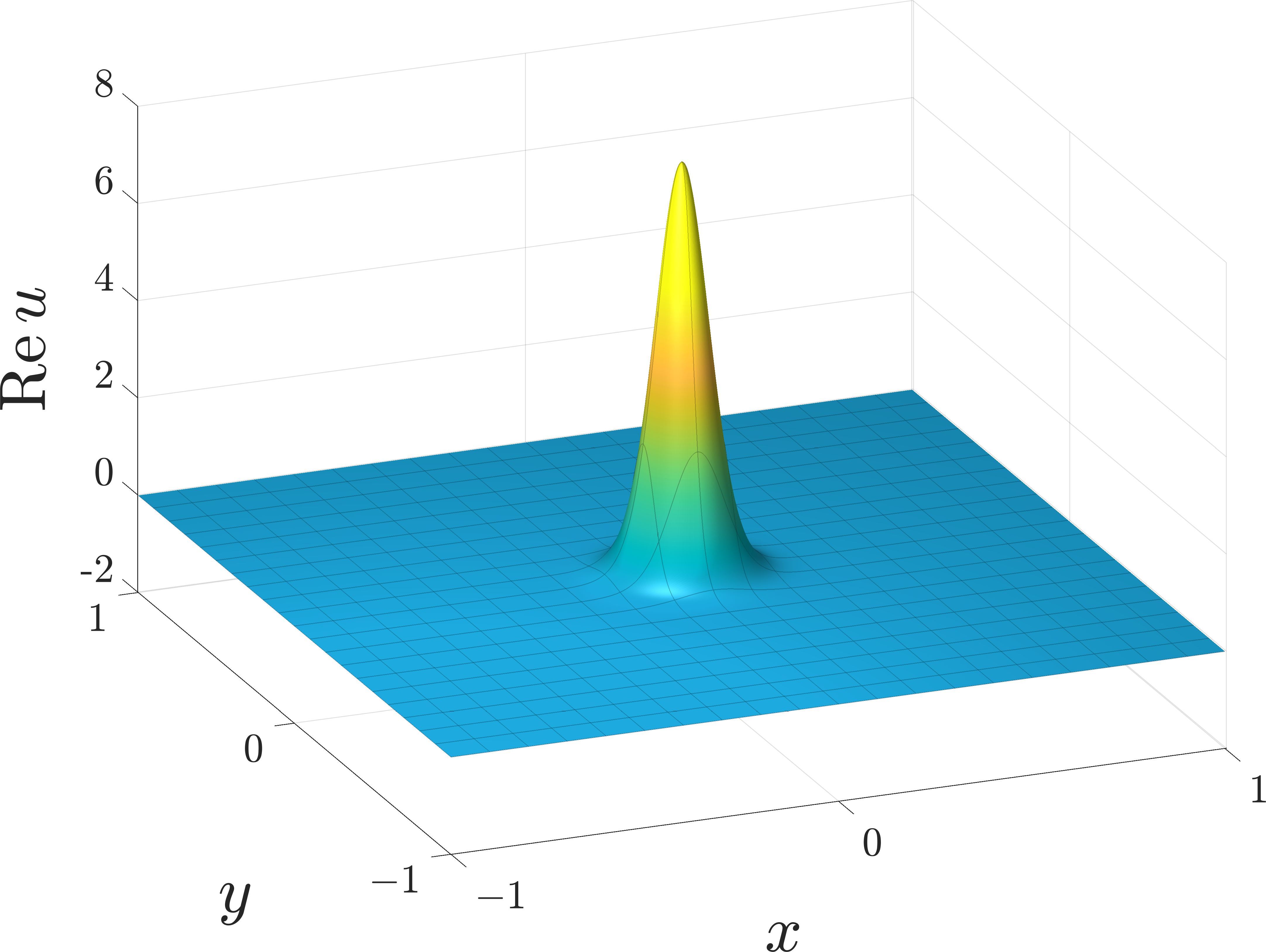
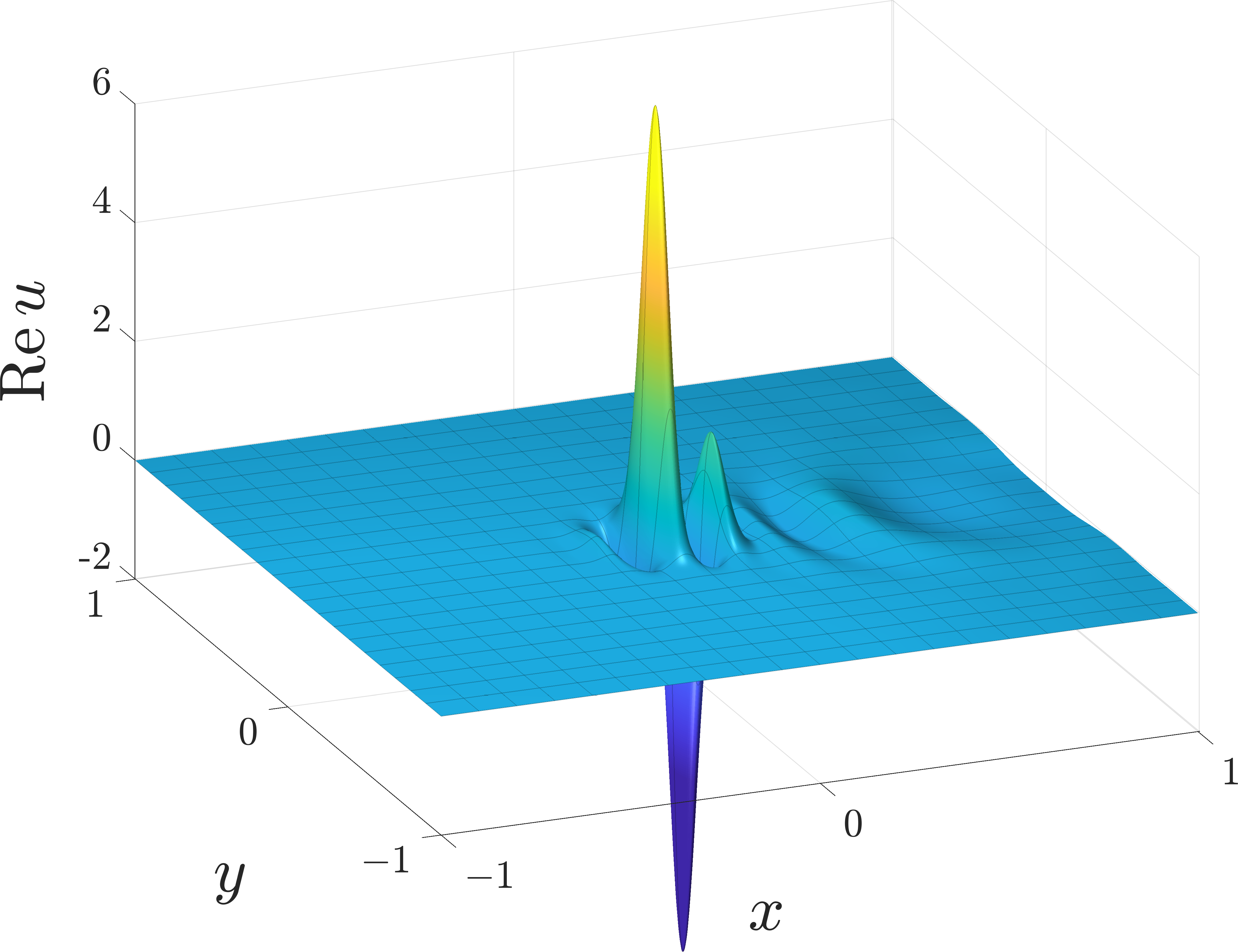
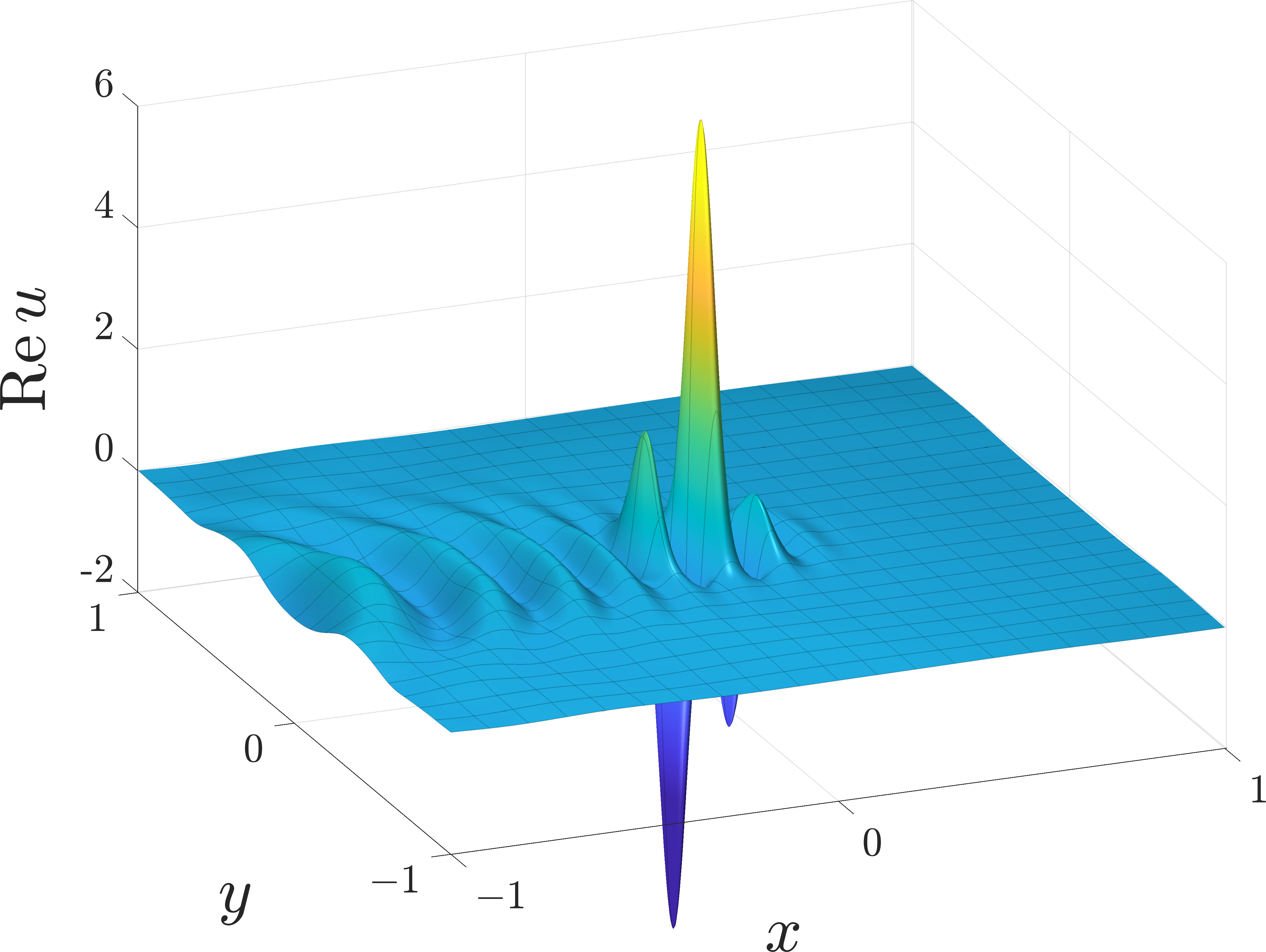
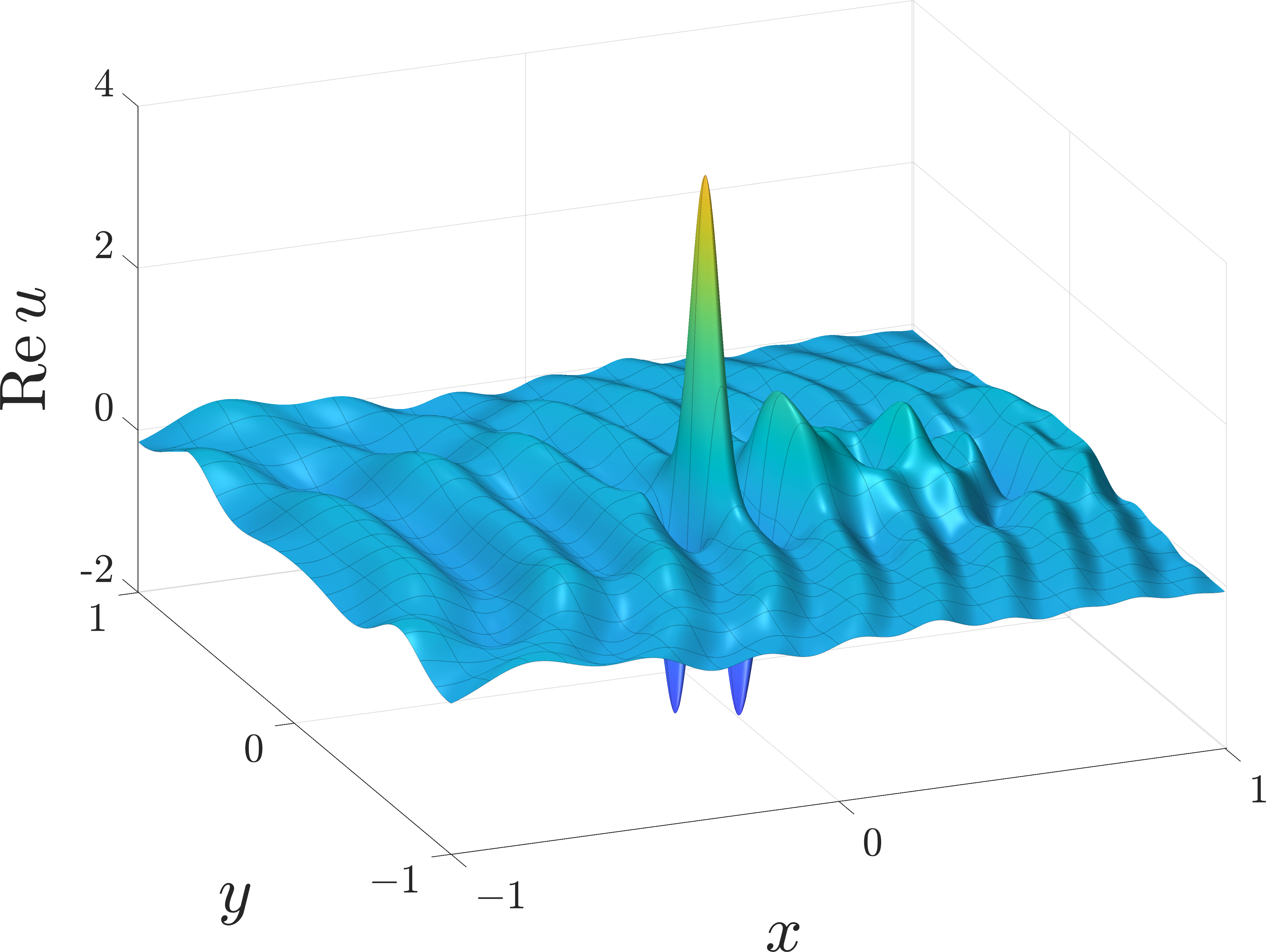
We again use the eighth-order implicit multistep scheme and fix , , and . As in Example 3, in the complex-frequency Fourier transform algorithm, -type transforms and transforms involving -type nodes are applied using direct multiplication rather than the Chebyshev interpolation scheme, since . We carry out higher accuracy calculations with , , and values of corresponding to 1000, 2000, 4000, …32000 time steps, and lower accuracy calculations with , , and values of corresponding to 1000, 2000, 4000, …16000 time steps. In Figure 11, the final-time errors , measured against a well-converged reference solution, are plotted against for several approximately logarithmically-spaced values of . Timings for each choice of and both choices of are given in Table 3.
| 0.3 | 0.5 | 0.9 | 1.4 | 2.4 | |
|---|---|---|---|---|---|
| Time steps per second, | 14 | 24 | 40 | 66 | 96 |
| Time steps per second, | 44 | 70 | 92 | 145 | 193 |
We remind the reader that increasing also increases and , so that the spectral Green’s function is less oscillatory along (see Figure 2). Thus and should be increased with to achieve the fastest computation for a given accuracy. In the experiment with , for example, to obtain approximately 10 digits of accuracy we set , , and take time steps at 14 time steps per second, whereas to obtain approximately 5 digits of accuracy, we can set , , and take time steps at 145 times steps per second.
7 Conclusion
We have introduced a Volterra integral equation-based numerical method for the periodic and free space TDSE with a spatially-uniform vector potential. The method offers several notable advantages compared with finite difference methods and methods based on applying the unitary single time step propagator. Namely, it permits inexpensive high-order implicit time stepping, naturally includes the case of time-dependent scalar potentials, and obviates the need for artificial boundary conditions in the free space case.
The Volterra integral equation involves a spacetime history-dependent volume integral, and we have used a Fourier method to avoid the computational cost and memory associated with its naive evaluation. This leads to a fast and memory-efficient FFT-based method, but requires the solution to be resolvable on a uniform grid in the physical domain. A new strategy will be required to make the integral equation formulation compatible with spatially-adaptive discretizations.
We note lastly that in practical applications, the scalar potential may be replaced by a somewhat more general object. In time-dependent density functional theory, for example, the potential is nonlinear and may be nonlocal. The integral equation approach enjoys several advantages over PDE-based methods in these cases, which will be explored in future work.
Acknowledgements
We thank Angel Rubio and Umberto de Giovannini for many useful discussions. J.K. was supported in part by the Research Training Group in Modeling and Simulation funded by the National Science Foundation via grant RTG/DMS-1646339. The Flatiron Institute is a division of the Simons Foundation.
Appendix A Proof of Lemma 3 for
Proof.
Fix and let be defined by the formula (27). It is well-defined and continuous in because and are entire functions of , and provides a proper extension of into the complex plane. The integral of around any closed contour in is zero—we can interchange the order of integration using Fubini’s theorem, and apply Cauchy’s theorem to the analytic integrand—so it follows from Morera’s theorem that is entire in .
To obtain (28) and (29), we write
where is the truncation of (26) to . We fix and choose to be either or . By Cauchy’s theorem, the classical inverse Fourier transforms (22) and (23) are equal to those taken along the deformed contour for any . The contributions from and vanish as because and , and therefore and , are in the Schwartz space. Thus to prove (28) and (29), we only need to show that the contributions from the two vertical segments and vanish in that limit, i.e.
for and . For the latter, we write
Here, noting that is smooth and compactly supported, we have used Fubini’s theorem to switch the order of integration. The inner integral is a smooth function, so the outer integral is the Fourier transform of a smooth, compactly supported function, evaluated at . The desired result then follows from the Riemann–Lebesgue lemma.
For , we instead use (18) to write
Let us consider the first term on the right hand side; the second may be dealt with by a similar approach. We again use Fubini’s theorem to obtain
| (69) |
We have for all and , where is given by (30). Therefore the inner integral defines a bounded, continuous function of . Since is a smooth function supported on , the outer integral is the Fourier transform of an integrable function evaluated at , and the result again follows from the Riemann–Lebesgue lemma. ∎
References
- [1] A. D. Bandrauk, F. Fillion-Gourdeau, and E. Lorin, “Atoms and molecules in intense laser fields: gauge invariance of theory and models,” J. Phys. B, vol. 46, no. 15, p. 153001, 2013.
- [2] C. Leforestier, R. Bisseling, C. Cerjan, M. Feit, R. Friesner, A. Guldberg, A. Hammerich, G. Jolicard, W. Karrlein, H.-D. Meyer, N. Lipkin, O. Roncero, and R. Kosloff, “A comparison of different propagation schemes for the time dependent Schrödinger equation,” J. Comput. Phys., vol. 94, no. 1, pp. 59–80, 1991.
- [3] S. Blanes and P. Moan, “Splitting methods for the time-dependent Schrödinger equation,” Phys. Lett. A, vol. 265, no. 1-2, pp. 35–42, 2000.
- [4] C. Lubich, “Integrators for quantum dynamics: a numerical analyst’s brief review,” in Quantum simulations of complex many-body systems: from theory to algorithms (J. Grotendorst, D. Marx, and A. Muramatsu, eds.), pp. 459–466, 2002.
- [5] K. Kormann, S. Holmgren, and H. O. Karlsson, “Accurate time propagation for the Schrödinger equation with an explicitly time-dependent Hamiltonian,” J. Chem. Phys., vol. 128, no. 18, p. 184101, 2008.
- [6] S. Blanes, F. Casas, and A. Murua, “An efficient algorithm based on splitting for the time integration of the Schrödinger equation,” J. Comput. Phys., vol. 303, pp. 396–412, 2015.
- [7] S. Blanes, F. Casas, and A. Murua, “Symplectic time-average propagators for the Schrödinger equation with a time-dependent Hamiltonian,” J. Chem. Phys., vol. 146, no. 11, p. 114109, 2017.
- [8] P. Bader, S. Blanes, and N. Kopylov, “Exponential propagators for the Schrödinger equation with a time-dependent potential,” J. Chem. Phys., vol. 148, no. 24, p. 244109, 2018.
- [9] A. Iserles, K. Kropielnicka, and P. Singh, “Magnus-Lanczos methods with simplified commutators for the Schrödinger equation with a time-dependent potential,” SIAM J. Numer. Anal., vol. 56, no. 3, pp. 1547–1569, 2018.
- [10] A. Castro, M. A. L. Marques, and A. Rubio, “Propagators for the time-dependent Kohn-Sham equations,” J. Chem. Phys., vol. 121, no. 8, pp. 3425–3433, 2004.
- [11] D. Kidd, C. Covington, and K. Varga, “Exponential integrators in time-dependent density-functional calculations,” Phys. Rev. E, vol. 96, p. 063307, 2017.
- [12] A. Gómez Pueyo, M. A. L. Marques, A. Rubio, and A. Castro, “Propagators for the time-dependent Kohn-Sham equations: multistep, Runge-Kutta, exponential Runge-Kutta, and commutator free Magnus methods,” J. Chem. Theory Comput., vol. 14, no. 6, pp. 3040–3052, 2018.
- [13] L. Lin and J. Lu, A Mathematical Introduction to Electronic Structure Theory. SIAM, 2019.
- [14] W. Magnus, “On the exponential solution of differential equations for a linear operator,” Commun. Pure Appl. Math., vol. 7, pp. 649–673, 1954.
- [15] A. Iserles, H. Z. Munthe-Kaas, S. P. Nørsett, and A. Zanna, “Lie-group methods,” Acta Numer., vol. 9, pp. 215–365, 2000.
- [16] S. Blanes, F. Casas, and J. Ros, “Improved high order integrators based on the Magnus expansion,” BIT Numer. Math., vol. 40, no. 3, pp. 434–450, 2000.
- [17] M. Hochbruck and C. Lubich, “On Magnus integrators for time-dependent Schrödinger equations,” SIAM J. Numer. Anal., vol. 41, no. 3, pp. 945–963, 2003.
- [18] A. M. Ermolaev, I. V. Puzynin, A. V. Selin, and S. I. Vinitsky, “Integral boundary conditions for the time-dependent Schrödinger equation: Atom in a laser field,” Phys. Rev. A, vol. 60, no. 6, p. 4831, 1999.
- [19] J. Kaye and L. Greengard, “Transparent boundary conditions for the time-dependent Schrödinger equation with a vector potential,” arXiv preprint arXiv:1812.04200, 2018.
- [20] A. D. Bandrauk, E. Dehghanian, and H. Lu, “Complex integration steps in decomposition of quantum exponential evolution operators,” Chem. Phys. Lett., vol. 419, no. 4-6, pp. 346–350, 2006.
- [21] F. Castella, P. Chartier, S. Descombes, and G. Vilmart, “Splitting methods with complex times for parabolic equations,” BIT Numer. Math., vol. 49, pp. 487–508, 2009.
- [22] E. Hansen and A. Ostermann, “High order splitting methods for analytic semigroups exist,” BIT Numer. Math., vol. 49, pp. 527–542, 2009.
- [23] S. Blanes, F. Casas, P. Chartier, and A. Murua, “Optimized high-order splitting methods for some classes of parabolic equations,” Math. Comput., vol. 82, no. 283, pp. 1559–1576, 2013.
- [24] A. Bourlioux, A. T. Layton, and M. Minion, “High-order multi-implicit spectral deferred correction methods for problems of reactive flow,” J. Comput. Phys., vol. 189, pp. 651–675, 2003.
- [25] A. J. Christlieb, Y. Liu, and Z. Xu, “High order operator splitting methods based on an integral deferred correction framework,” J. Comput. Phys., vol. 294, pp. 224–242, 2015.
- [26] M. Duarte and M. Emmett, “High order schemes based on operator splitting and deferred corrections for stiff time dependent PDEs,” arXiv preprint arXiv:1407.0195v2, 2016.
- [27] T. Hagstrom and R. Zhou, “On the spectral deferred correction of splitting methods for initial value problems,” Comm. App. Math. and Comp. Sci., vol. 1, pp. 169–205, 2006.
- [28] C. Zhang, J. Huang, C. Wang, and X. Yue, “On the operator splitting and integral equation preconditioned deferred correction methods for the ‘good’ Boussinesq equation,” J. Sci. Comput., vol. 75, pp. 687–712, 2018.
- [29] R. J. LeVeque, Finite Difference Methods for Ordinary and Partial Differential Equations. SIAM, 2007.
- [30] U. De Giovannini, A. H. Larsen, and A. Rubio, “Modeling electron dynamics coupled to continuum states in finite volumes with absorbing boundaries,” Eur. Phys. J. B, vol. 88, no. 3, p. 56, 2015.
- [31] M. Weinmüller, M. Weinmüller, J. Rohland, and A. Scrinzi, “Perfect absorption in Schrödinger-like problems using non-equidistant complex grids,” J. Comput. Phys., vol. 333, pp. 199–211, 2017.
- [32] X. Antoine, E. Lorin, and Q. Tang, “A friendly review of absorbing boundary conditions and perfectly matched layers for classical and relativistic quantum waves equations,” Mol. Phys., vol. 115, no. 15-16, pp. 1861–1879, 2017.
- [33] V. A. Baskakov and A. V. Popov, “Implementation of transparent boundaries for numerical solution of the Schrödinger equation,” Wave Motion, vol. 14, no. 2, pp. 123–128, 1991.
- [34] C. Lubich and A. Schädle, “Fast convolution for non–reflecting boundary conditions,” SIAM J. Sci. Comput., vol. 24, pp. 161–182, 2002.
- [35] S. Jiang and L. Greengard, “Fast evaluation of nonreflecting boundary conditions for the Schrödinger equation in one dimension,” Comput. Math. Appl., vol. 47, no. 6, pp. 955–966, 2004.
- [36] A. Schädle, M. López-Fernández, and C. Lubich, “Fast and oblivious convolution quadrature,” SIAM J. Sci. Comput., vol. 28, no. 2, pp. 421–438, 2006.
- [37] H. Han and Z. Huang, “Exact artificial boundary conditions for the Schrödinger equation in ,” Commun. Math. Sci., vol. 2, no. 1, pp. 79–94, 2004.
- [38] S. Jiang and L. Greengard, “Efficient representation of nonreflecting boundary conditions for the time-dependent Schrödinger equation in two dimensions,” Commun. Pure Appl. Math., vol. 61, no. 2, pp. 261–288, 2008.
- [39] H. Han, D. Yin, and Z. Huang, “Numerical solutions of Schrödinger equations in ,” Numer. Methods Partial Differ. Equ., vol. 23, no. 3, pp. 511–533, 2007.
- [40] R. M. Feshchenko and A. V. Popov, “Exact transparent boundary condition for the parabolic equation in a rectangular computational domain,” J. Opt. Soc. Am. A, vol. 28, pp. 373–380, 2011.
- [41] R. M. Feshchenko and A. V. Popov, “Exact transparent boundary condition for the three-dimensional Schrödinger equation in a rectangular cuboid computational domain,” Phys. Rev. E, vol. 88, p. 053308, 2013.
- [42] A. Schädle, “Non-reflecting boundary conditions for the two-dimensional Schrödinger equation,” Wave Motion, vol. 35, no. 2, pp. 181–188, 2002.
- [43] E. Lorin, S. Chelkowski, and A. Bandrauk, “Mathematical modeling of boundary conditions for laser-molecule time-dependent Schrödinger equations and some aspects of their numerical computation—one-dimensional case,” Numer. Methods Partial Differ. Equ., vol. 25, no. 1, pp. 110–136, 2009.
- [44] V. Vaibhav, “Transparent boundary condition for numerical modeling of intense laser–molecule interaction,” J. Comput. Phys., vol. 283, pp. 478–494, 2015.
- [45] R. M. Feshchenko and A. V. Popov, “Exact transparent boundary conditions for the parabolic wave equations with linear and quadratic potentials,” Wave Motion, vol. 68, pp. 202–209, 2017.
- [46] B. Engquist and A. Majda, “Absorbing boundary conditions for the numerical simulation of waves,” Math. Comput., vol. 31, no. 139, pp. 629–651, 1977.
- [47] X. Antoine and C. Besse, “Construction, structure and asymptotic approximations of a microdifferential transparent boundary condition for the linear Schrödinger equation,” J. Math. Pures Appl., pp. 701–738, 2001.
- [48] X. Antoine, C. Besse, and V. Mouysset, “Numerical schemes for the simulation of the two-dimensional Schrödinger equation using non-reflecting boundary conditions,” Math. Comput., vol. 73, no. 248, pp. 1779–1799, 2004.
- [49] X. Antoine, A. Arnold, C. Besse, M. Ehrhardt, and A. Schädle, “A review of transparent and artificial boundary conditions techniques for linear and nonlinear Schrödinger equations,” Commun. Comput. Phys., vol. 4, no. 4, pp. 729–796, 2008.
- [50] A. Arnold, M. Ehrhardt, and I. Sofronov, “Discrete transparent boundary conditions for the Schrödinger equation: fast calculation, approximation and stability,” Commun. Math. Sci, vol. 1, no. 3, pp. 501–556, 2003.
- [51] A. Arnold, M. Ehrhardt, M. Schulte, and I. Sofronov, “Discrete transparent boundary conditions for the Schrödinger equation on circular domains,” Commun. Math. Sci., vol. 10, no. 3, pp. 889–916, 2012.
- [52] S. Ji, Y. Yang, G. Pang, and X. Antoine, “Accurate artificial boundary conditions for the semi-discretized linear Schrödinger and heat equations on rectangular domains,” Comput. Phys. Commun., vol. 222, pp. 84–93, 2018.
- [53] D. K. Hoffman, O. A. Sharafeddin, R. S. Judson, and D. J. Kouri, “Time-dependent treatment of scattering: Integral equation approaches using the time-dependent amplitude density,” J. Chem. Phys., vol. 92, no. 7, pp. 4167–4177, 1990.
- [54] O. A. Sharafeddin, D. J. Kouri, R. S. Judson, and D. K. Hoffman, “Time dependent integral equation approaches to quantum scattering: Comparative application to atom–rigid rotor multichannel scattering,” J. Chem. Phys., vol. 96, no. 7, pp. 5039–5046, 1992.
- [55] J. P. Boyd, Chebyshev and Fourier Spectral Methods. Dover, 2001.
- [56] L. N. Trefethen, Approximation Theory and Approximation Practice. SIAM, 2013.
- [57] J. F. Epperson, “Semigroup linearization for nonlinear parabolic equations,” Numer. Methods Partial Differ. Equ., vol. 7, no. 2, pp. 147–163, 1991.
- [58] J. Strain, “Fast adaptive methods for the free-space heat equation,” SIAM J. Sci. Comput., vol. 15, no. 1, pp. 185–206, 1994.
- [59] J. Wang, L. Greengard, S. Jiang, and S. Veerapaneni, “Fast integral equation methods for linear and semilinear heat equations in moving domains,” arXiv preprint arXiv:1910.00755, 2019.
- [60] L. N. Trefethen and J. Weideman, “The exponentially convergent trapezoidal rule,” SIAM Rev., vol. 56, no. 3, pp. 385–458, 2014.
- [61] G. Dahlquist and A. Björck, Numerical Methods in Scientific Computing: Volume 1, vol. 103. SIAM, 2008.
- [62] L. Greengard and P. Lin, “Spectral approximation of the free-space heat kernel,” Appl. Comput. Harmon. Anal., vol. 9, no. 1, pp. 83–97, 2000.
- [63] R. Strichartz, A guide to distribution theory and Fourier transforms. CRC Press, 1994.
- [64] A. Barnett and L. Greengard, “A new integral representation for quasi-periodic scattering problems in two dimensions,” BIT Numer. Math., vol. 51, no. 1, pp. 67–90, 2011.
- [65] A. Dutt and V. Rokhlin, “Fast Fourier transforms for nonequispaced data,” SIAM J. Sci. Comput., vol. 14, pp. 1368–1393, 1993.
- [66] L. Greengard and J.-Y. Lee, “Accelerating the nonuniform fast Fourier transform,” SIAM Rev., vol. 46, no. 3, pp. 443–454, 2004.
- [67] A. H. Barnett, J. Magland, and L. af Klinteberg, “A parallel nonuniform fast Fourier transform library based on an ‘exponential of semicircle’ kernel,” SIAM J. Sci. Comput., vol. 41, no. 5, pp. C479–C504, 2019.
- [68] B. K. Alpert, “Hybrid Gauss-trapezoidal quadrature rules,” SIAM J. Sci. Comput., vol. 20, no. 5, pp. 1551–1584, 1999.
- [69] M. Frigo and S. G. Johnson, “The design and implementation of FFTW3,” Proc. IEEE, vol. 93, no. 2, pp. 216–231, 2005.
- [70] T. A. Driscoll, F. Bornemann, and L. N. Trefethen, “The chebop system for automatic solution of differential equations,” BIT Numer. Math., vol. 48, no. 4, pp. 701–723, 2008.