The Low Effective Spin of Binary Black Holes and Implications for Individual Gravitational-Wave Events
Abstract
While the Advanced LIGO and Virgo gravitational-wave experiments now regularly observe binary black hole mergers, the evolutionary origin of these events remains a mystery. Analysis of the binary black hole spin distribution may shed light on this mystery, offering a means of discriminating between different binary formation channels. Using the data from Advanced LIGO and Virgo’s first and second observing runs, here we seek to carefully characterize the distribution of effective spin among binary black holes, hierarchically measuring the distribution’s mean and variance while accounting for selection effects and degeneracies between spin and other black hole parameters. We demonstrate that the known population of binary black holes have spins that are both small, with , and very narrowly distributed, with at 95% credibility. We then explore what these ensemble properties imply about the spins of individual binary black hole mergers, re-analyzing existing gravitational-wave events with a population-informed prior on their effective spin. Under this analysis, the binary black hole GW170729, which previously excluded , is now consistent with zero effective spin at credibility. More broadly, we find that uninformative spin priors generally yield overestimates for the effective spin magnitudes of compact binary mergers.
I Introduction
In their first two observing runs, the Advanced LIGO (Laser Interferometer Gravitational-wave Observatory) and Advanced Virgo experiments (Aasi et al. 2015; Acernese et al. 2015) have detected gravitational waves from eleven compact binary coalescences - ten binary black hole (BBH) mergers and one binary neutron star (BNS) merger (Abbott et al. 2016a; Abbott et al. 2017; Abbott et al. 2019a). This early catalog of gravitational-wave (GW) signals has already been used to measure a diverse set of physical parameters, from the binaries’ component masses and spins (Abbott et al. 2016b; Abbott et al. 2019b; Abbott et al. 2019a; Chatziioannou et al. 2019; Kimball et al. 2019) to more complex phenomena such as tidal effects (Abbott et al. 2018a; Raithel et al. 2018) and consistency with general relativity (Abbott et al. 2016c; Abbott et al. 2019c; Abbott et al. 2019d).
The number of gravitational-wave detections is rapidly growing. Now roughly halfway through their third “O3” observing run, LIGO and Virgo have already reported new detection candidates; together with the newly-built KAGRA detector (Aso et al. 2013), they are expected to observe an additional events in O4 (Abbott et al. 2018b). As the number of gravitational-wave detections increases, we can shift our focus from the study of individual binaries to the analysis of their ensemble (Abbott et al. 2016a; Abbott et al. 2019e). While the astrophysical details of compact binary evolution are only weakly reflected in the properties of individual events, we expect them to much more strongly inform binaries’ population properties – the distributions of component masses, spins, and redshifts. Uncovering these ensemble properties is therefore a promising means of determining which evolutionary channel drives the formation of compact binary mergers: the evolution of isolated stellar binaries, dynamical capture in dense stellar environments, or yet another channel altogether.
In this paper, we will explore the distribution of binary black hole spins detected by Advanced LIGO and Virgo. Ours is not the first attempt at such an analysis – several authors have previously explored the binary black hole spin distribution, using varying subsets of the LIGO and Virgo detections and employing a range of different models. Our goals in this work are threefold:
1. Focus on the observable. Many previous studies aim to describe the distributions of spin magnitudes and/or tilt angles of the individual black holes comprising the observed BBH population (Talbot & Thrane 2017; Farr et al. 2017; Farr et al. 2018; Tiwari et al. 2018; Fernandez & Profumo 2019; Wysocki et al. 2019; Stevenson et al. 2017; Abbott et al. 2019e; Roulet & Zaldarriaga 2019). Gravitational waves carry relatively little information, however, about the spins of these individual components. At leading order, gravitational-wave signals instead depend only on a single effective spin parameter , quantifying the net projection of both component spins onto a binary’s orbital angular momentum (Damour 2001; Racine 2008; Ajith et al. 2011; Ng et al. 2018; Roulet & Zaldarriaga 2019). We will therefore not attempt to model the ensemble of underlying component spins, but instead seek to describe the more readily-measurable distribution (Farr et al. 2017; Farr et al. 2018; Tiwari et al. 2018; Roulet & Zaldarriaga 2019).
2. Adopt a simple population model. Popular models for the binary black hole spin distribution are often rather complex. The flagship LIGO/Virgo analysis, for example, employs a flexible five-parameter model to describe the ensemble of black hole spins (Abbott et al. 2019e). With only ten detections information these measurements, the resulting constraints from such models are generally uninformative. Here, we will instead adopt a deliberately simple model, characterizing the distribution via only two parameters: its mean and variance. While this choice sacrifices some flexibility, it will yield transparent and intuitive results that are more robustly extracted from presently small number of gravitational-wave events.
3. Account for observational biases. The underlying distribution is observationally obscured in two ways. The first is selection bias – more highly spinning binary systems accumulate more gravitational-wave cycles, and are thus preferentially detected with higher signal-to-noise ratios. The second is potential measurement degeneracy between effective spin and other binary parameters, most notably the mass ratio (Ng et al. 2018). Previous analyses variously do (Tiwari et al. 2018; Roulet & Zaldarriaga 2019; Abbott et al. 2019e) and do not (Farr et al. 2017; Farr et al. 2018; Fernandez & Profumo 2019) account for these spin-dependent effects.
Just as individual binary black holes inform measurements of the population’s spin distribution, so too can knowledge of the spin distribution inform our conclusions about individual events. After hierarchically measuring the binary black hole distribution (Sec. III), we will therefore turn around and use this information to re-analyze the ten LIGO/Virgo detections, producing updated measurements of their effective spins (Sec. IV).
II Hierarchical Inference of Black Hole Spins
At leading order, the amplitude and phase evolution of a binary’s gravitational-wave signal depend on its component spin through two parameters: the “effective” and “precessing” spins, and (Ajith et al. 2011; Schmidt et al. 2015). The effective spin , a unitless quantity between and , is the mass-weighted average of the dimensionless component spins and , projected along the unit vector parallel to the system’s orbital angular momentum:
| (1) |
Here, are the source-frame masses of each black hole such that . The effective spin may also be expressed in terms of the component spin magnitudes and tilt angles between each spin and :
| (2) |
, on the other hand, is a unitless value between 0 and 1 that parametrizes the leading-order effects of orbital precession due to misaligned spins. While is related to the spin components parallel to , is a linear combination of spin components normal to .
In this paper, we will focus on understanding the distribution of across the population of merging stellar-mass black holes. In contrast to more complex, many-parameter models featured in previous work (Abbott et al. 2019e; Wysocki et al. 2019), we will assume that effective spins are drawn from a simple truncated Gaussian,
| (3) |
and to seek to measure the mean and variance of this ensemble distribution. The normalization constant
| (4) |
ensures that Eq. (3) is properly normalized over the range .
Although is measured far more precisely than the individual component spins, it is still subject to significant uncertainty (Ng et al. 2018; Abbott et al. 2019a). More specifically, for each gravitational-wave signal (with associated data ), we do not obtain a direct point estimate of , but instead a set of discrete samples from the posterior probability distribution for the effective spin. We must therefore employ a hierarchical approach in which each LIGO/Virgo BBH event is assumed to have some true but unknown value of drawn from Eq. (3) above. We will marginalize over the possible of each LIGO/Virgo event to obtain a posterior on the mean and variance of the population’s effective spin distribution.
Given independent binary black hole detections (in our case ) with population-averaged detection efficiency and data , the resulting posterior distribution for and is given in Eq. (5) (Loredo & Wasserman 1995; Loredo 2004; Fishbach et al. 2018; Mandel et al. 2019). The first line corresponds to the ideal case in which the posterior on each event’s effective spin, component masses, and redshift are exactly known; the second line is for the realistic scenario in which we have only discrete samples from the posterior of every event.
| (5) | ||||
The effective spin samples generated by parameter estimation are necessarily obtained under the assumption of some default prior . The LIGO/Virgo samples produced by the LALInference software (Veitch et al. 2015; LIGO Scientific Collaboration 2019), for instance, are given by priors that are uniform in component spin magnitude and orientation, such that and are both constant. This corresponds to a symmetric prior that is broady peaked about zero. In Eq. (5) we must “undo” this default prior and reweight each sample by the proposed Gaussian distribution , evaluated at the given sample value ).
LALInference also imposes a computationally-simple but unphysical prior on the component masses and redshift of a binary black hole merger. Specifically, uniform priors are adopted for the detector frame masses and as well as the luminosity distance . This translates into (Abbott et al. 2019e)
| (6) |
Here, is the comoving distance at redshift and is the speed of light. is the Hubble parameter, given by the present-day Hubble constant km/s/Mpc and energy densities and of mass and dark energy, respectively (Ade et al. 2016). Although total mass is not strongly correlated with , is generally anti-correlated with a binary’s mass ratio , as shown in Roulet & Zaldarriaga 2019, for example. The default LALInference priors are uniform in detector-frame component masses, and thus preferentially tolerate systems with unequal mass ratios, thereby pushing posteriors to larger values (Ng et al. 2018; Tiwari et al. 2018). We compensate for this potential bias in Eq. (5) by further reweighting LALInference samples by an astrophysically-motivated mass and redshift prior, consistent with the measured mass and redshift distributions of binary black holes following the second Advanced LIGO/Virgo observing run (Abbott et al. 2019e):
| (7) |
This prior is logarithmically-uniform in primary mass and uniform in mass-ratio, and assumes a binary merger rate that follows star formation, growing as in the source frame (Madau & Dickinson 2014). In our detector frame, the measured merger rate is redshifted to . is the comoving volume per unit redshift, and we assume a minimum black hole mass . We do not impose a maximum mass cutoff.
Observational selection effects are accounted for in Eq. (5) by the population-averaged detection efficiency , the fraction of all BBH mergers that LIGO successfully detects:
| (8) |
where is the probability, marginalized over all other parameters, that we will detect a BBH with a given . In practice, we compute via the Monte Carlo approach of Farr 2019, drawing synthetic BBHs with random orientations, masses and redshifts following Eq. (7), and effective spins from a flat reference distribution . We compute the Advanced LIGO matched filter signal-to-noise ratio for each synthetic BBH using the “Early High-Sensitivity” power spectral density of Abbott et al. 2018b and the precessing IMRPhenomPv2 waveform model (Hannam et al. 2014), although we assume purely aligned spins. Events with in the Advanced LIGO detector network are considered to have been “detected.” Figure 1 shows a histogram of the effective spins for these mock detections; at current sensitivities, we see that Advanced LIGO is roughly five times more likely to detect a maximally aligned system () than a maximally anti-aligned system (). Given a proposed mean and variance of the distribution, the corresponding detection fraction can then be evaluated as a reweighted sum over our catalog of synthetic “detections” (Farr 2019),
| (9) |
where is the total number of synthetic events, is the number of “detections,” and is the effective spin of the detected event.
Finally, we note that Eq. (5) does not depend on the overall rate of black hole mergers. As we are concerned only with the shape of the distribution and not the absolute number distribution of mergers, Eq. (5) is derived by marginalizing over the total event rate, assuming a logarithmically uniform rate prior (Fishbach et al. 2018; Mandel et al. 2019).
III Results from O1 and O2 Detections
We analyze the ten binary black hole mergers reported by LIGO and Virgo in their O1 and O2 observing runs (Abbott et al. 2019a; LIGO Scientific Collaboration & Virgo Collaboration 2019). Before discussing results, it is useful to review expectations from the literature for the spin distributions resulting from different formation scenarios. Isolated binary evolution is predicted to yield black hole with spins preferentially aligned with their orbit. Although spin misalignments may be introduced by natal supernova kicks, episodes of mass transfer and tidal torques serve to realign component spins before the formation of the final black hole binary (Rodriguez et al. 2016; Zevin et al. 2017; Gerosa et al. 2018; Qin et al. 2018; Zaldarriaga et al. 2018; Bavera et al. 2019). The black holes’ spin magnitudes in this scenario are much more uncertain. Recent work indicates that angular momentum is efficiently transported away from stellar cores, leaving black holes with natal spins as low as (Qin et al. 2018; Fuller & Ma 2019). While tides on the progenitor of the second-born black hole can spin up the progenitor star (Zaldarriaga et al. 2018), this effect can be counteracted by mass loss in stellar winds, and more detailed simulations find only low or moderate spin increases due to tides (Qin et al. 2018; Bavera et al. 2019). Meanwhile, dynamically-formed systems in dense stellar clusters have no a priori preferred axis, and so are likely to have random spin configurations (Rodriguez et al. 2016; Rodriguez et al. 2018; Doctor et al. 2019; Rodriguez et al. 2019). Once again, however, the expected spin magnitudes are largely unknown, subject to the same uncertainties mentioned above regarding natal black hole spins. One firm prediction of the dynamical scenario concerns the spins of second-generation binaries, whose components were themselves formed from previous mergers. Regardless of their component spins, black hole mergers generally yield remnants with ; thus the effective spin of two such second-generation binaries may be large (Fishbach et al. 2017; Gerosa & Berti 2017; Rodriguez et al. 2018; Doctor et al. 2019; Rodriguez et al. 2019).
In summary, the most robust discriminator between the isolated binary and dynamical scenarios is the mean of the effective spin distribution. If isolated binaries have preferentially aligned spins, then we expect an effective spin distribution centered on a positive value: . Dynamically-formed binaries with random spin orientations, meanwhile, should have a symmetric distribution centered at (Farr et al. 2018).
To generate our posterior distributions for and , we sample from Eq. 5 using emcee, a Markov Chain Monte Carlo (MCMC) package in Python (Foreman-Mackey et al. 2013). We use the public LALInference samples made available through the Gravitational Wave Open Science Center (Vallisneri et al. 2015; LIGO Scientific Collaboration & Virgo Collaboration 2019). Specifically, we use the so-called “overall posterior” samples, which are a union of the samples obtained with the IMRPhenomPv2 (Hannam et al. 2014) and SEOBNRv3 (Taracchini et al. 2014; Pan et al. 2014) waveform models; we have confirmed that our results are robust under the use of either waveform model independently. We adopt flat priors across the ranges and . Our posterior on and is given in Fig. 2. With the ten binary black holes observed in O1 and O2 by Advanced LIGO and Virgo, we constrain the mean of the binary black hole distribution to . Hence we find no evidence for preferential spin alignment, which would manifest as preferentially positive . Meanwhile, we find that width of the distribution must be extremely small, with a variance at 95% credibility. Curiously, provided that is nonzero, the data are consistent with a vanishingly narrow spin distribution. This can be seen in Fig. 2, which does not exclude . We therefore cannot yet rule out the possibility that the distribution is a delta function, with all binary black holes sharing the same effective spin value.
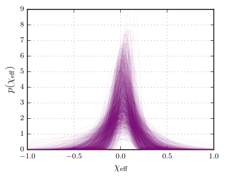
In Fig. 3, we plot the ensemble of permitted distributions consistent with our posterior on and . This figure again shows our slight preference for positive , but primarily illustrates that all distributions consistent with the presently-known binary black hole mergers must be narrowly peaked about .
Such small effective spins likely indicate one of three possibilities. First, these results are compatible with a scenario in which component spins are large but preferentially lie in the plane perpendicular to the binary’s orbital angular momentum. Intriguingly, some models for binary mergers driven by Kozai-Lidov resonances (Kozai 1962; Lidov 1962) in hierachical triples predict preferentially perpendicular spins (Rodriguez & Antonini 2018; Antonini et al. 2018; Liu & Lai 2018), although this effect is not observed in all studies (Antonini et al. 2018; Liu et al. 2019). Second, all component spins could be large but primarily anti-aligned with one another, such that each spin cancels the other’s contribution to Eq. (1); we are not aware of any merger channels that predict this. (Note, however, that BBH formation in the disks of active galactic nuclei may lead to the unique possibility of anti-aligned spins in approximately half of the BBH population (McKernan et al. 2019; Yang et al. 2019)). Finally, as has been noted by other authors, these results may point to the simple fact that binary black hole component spins are intrinsically small (Farr et al. 2017; Tiwari et al. 2018; Wysocki et al. 2019). This final scenario would yield a distribution concentrated around zero, regardless of spin orientation. By positing small natal spins, models of isolated field binaries (Belczynski et al. 2017; Postnov & Kuranov 2019), dynamical formation (Rodriguez et al. 2019), and hierarchical triples (Antonini et al. 2018) can all produce distributions like those shown in Fig. 3.
Given the theoretical uncertainties in spin magnitude, some authors have suggested that, rather than and , a more robust prediction might be the fraction of black hole binaries with negative (Rodriguez et al. 2016; Gerosa et al. 2018). In Fig. 4, we show posteriors on the fractions of binaries with positive and negative effective spins. We follow Farr et al. 2018 and Abbott et al. 2019e in additionally defining a third “uninformative” bin , with , in which effective spins are essentially indistinguishable from zero. At 95% credibility, a fraction of binaries are expected to have uninformatively small effective spins. Of the informative events, are predicted to have negative spins. Notably, however, the posteriors in Fig. 4 do not exclude the possibility of no detectably-negative effective spins; instead we can only confidently limit the fraction of detectably negative effective spins to at 95% credibility. These results differ from Abbott et al. 2019e, which reports that 80% of BBH have uninformatively small spins. This difference can be attributed to two possibilities. First, if the true distribution is narrower than we can presently resolve with 10 events, then our Gaussian model will generally overestimate the width of the distribution, thereby underestimating the fraction of uninformative events. Alternatively, if the width of the true distribution is comparable to or larger than , then the piecewise “three-bin” model of Farr et al. 2018 and Abbott et al. 2019e is a poor representation of the true underlying distribution, and will generally overestimate the fraction of uninformative events in the central bin. We may be seeing the effects of one or both of these possibilities, since they are not mutually exclusive.
It is worth noting that Roulet & Zaldarriaga 2019 have also explored a Gaussian model for the binary black hole distribution, obtaining constraints on consistent with ours when analyzing the GWTC-1 catalogue. Our measurement of , however, qualitatively differs from their results. Where our posterior permits extremely small , Roulet & Zaldarriaga 2019’s results exclude a vanishingly narrow distribution. This distinction could be due to a number of differences between our two analyses. First, while both analyses adopt a uniform prior in mass ratio, Roulet & Zaldarriaga 2019 additionally assume a uniform prior in chirp mass, while our prior is logarithmically uniform in primary mass. We have verified, though, that the adoption of a uniform-in-chirp-mass prior does not affect our results. Second, perhaps more significantly, to generate generate posteriors on and , Roulet & Zaldarriaga 2019 rely on analytic likelihood evaluations performed under a number of simplifying assumptions, such as the perfect alignment of all component spins. On the other hand, we use posterior distributions sampled by MCMC methods. Finally, Roulet & Zaldarriaga 2019 evaluate the detection efficiency via direct integration, whereas again we take a Monte Carlo approach as described above. A consequence of our Monte Carlo method is that, numerically speaking, we cannot sample arbitrarily close to . As approaches zero, the detection efficiency vanishes and the likelihood diverges to infinity. To prevent this divergence, we impose the stability condition recommended in Farr 2019 – that the number of synthetic detections contributing to Eq. (9) be greater than (where is our number of real events). This condition prevents us from sampling variances below ; even at , though, our posterior remains flat.
IV Refined Binary Black Hole Spin Measurements

Given what we now know about the population distribution of , we can obtain refined measurements on each individual binary black hole system. As described in Sec. II, the default LALInference priors on component spins are uniform in dimensionless magnitude and isotropic in direction. Having obtained information about the actual population distribution of , we can replace the uninformative LALInference prior with one that matches the recovered distribution. Specifically, we will recompute the posterior on the effective spin of each of the ten binary black hole detections, marginalizing over all possible values of and . We will additionally undo the default LALInference mass and redshift priors, reweighting by our astrophysically-motivated prior in Eq. (7).
For brevity, we’ll introduce the abbreviation for the set of parameters describing an individual compact binary. Given the complete set for all our events, we can form a joint posterior on , , and the parameters of some single event:
| (10) |
This is simply Eq. (5), absent marginalization over the single event of interest. Equation (10) can be put into a more convenient form if we multiply and divide by . This gives
| (11) | ||||
This expression now depends only on the default posterior for the event of interest and the marginal posterior on the population parameters given all events – exactly what we computed above in Sect. II.
Given discrete samples from and , we can sample Eq. (10) via a two step procedure, in which we (i) select a posterior sample from , then (ii) select a random parameter estimation sample , subject to the weights
| (12) | ||||
Equation (11) contains an extra factor, , that does not appear in the above weights. This is because, once we condition on the particular values and , the factor appearing in Eq. (11) is a constant; we can therefore neglect it from the weights in Eq. (12).
For each of the ten binary black holes detected in O1 and O2 by Advanced LIGO Virgo, Fig. 5 compares the default LALInference posteriors to our population-informed posteriors. The LALInference posteriors are shaded, while the population-informed posteriors are in white. In all cases the population-informed prior serves to shift each posterior distribution towards . This shift operates in both directions – posteriors that strongly support positive are moved downward, while posteriors supporting negative effective spins shift up. This “shrinkage” effect is common to hierarchical models of observations with significant uncertainty (Lieu et al. 2017). GW170729, for example, excludes with 99% credibility when using uninformative priors. The population-informed prior, though, noticeably shifts the GW170729’s posterior downward; 8% of the posterior now extends below and the peak is lowered from to . The effective spin of GW151226, on the other hand, remains confidently positive, with at 99% credibility under both the uninformative and population-informed priors. GW170818, meanwhile, originally shows moderate support for negative effective spins, with 77% of the posterior at . Under our population-informed prior, 68% of GW170818’s prior now supports negative values.
A key takeaway from these results is that when a collection of binary black holes are analyzed in isolation under default priors common to such analyses, the magnitude of their effective spins will be consistently overestimated. When studying future compact binary mergers, it will be essential to evaluate their spins in the context of the broader population, particularly when an event seemingly has confidently positive or negative . Further updated population-informed posteriors on the parameters of individual gravitational wave events are given in Fishbach et al. 2019 and Galaudage et al. 2019.
V Conclusion
As we enter deeper into the era of gravitational-wave astronomy, increasingly valuable information will be encoded in the ensemble properties of compact binary mergers. The distribution of parameters like mass, spin, and redshift across the observable universe’s binary black hole population contain essential information about the formation and evolutionary pathways of such systems. We focus on the population distribution for effective spin, . This parameter characterizes gravitational-wave strain at leading order, and is thus easily accessible from the data from the small number of LIGO/Virgo events. Additionally, our focus on this single phenomenological parameter provides a simple and intuitive framework on which future analyses can be built. In a complementary paper, for example, Safarzadeh et al. 2020 extend our model to investigate correlations between the effective spins and masses of binary black holes.
In this paper, we have explored the distribution of the effective spin parameter across the ten binary black holes observed by LIGO and Virgo in their O1 and O2 observing run. We adopted a simple and intuitive model, measuring the mean and variance of effective spins across this ensemble of gravitational-wave events,and rigorously accounting for observational selection effects and degeneracies. At 95% credibility, we found and . Notably, is consistent with , meaning that the distribution of BBH effective spins is consistent with a delta function. As discussed in Sec. III, it is not clear whether this result preferentially supports a dynamical or field binary origin (or even other possibilities) for stellar-mass binary black holes. Instead, this result likely indicates that binary black holes have small spin magnitudes, far smaller than those inferred in x-ray binaries (Miller & Miller 2015).
Our knowledge of the ensemble distribution of , in turn, allowed us to refine measurements for individual binary black hole events. Existing spin measurements were obtained under an uninformative prior on component spin magnitudes and orientations. Here, we instead used our measurements of and to generate a population-informed prior, which we used to reweight existing parameter estimation results for the ten O1 and O2 binary black hole detections. Using our population-informed prior, the resulting effective spin posteriors are all shifted towards . In some cases this shift is significant. For example, GW170729 previously excluded at 99% credibility. Under a population-informed prior, however, it shows a probability for zero (or negative) effective spin. More broadly, our results demonstrate the value of analyzing the ensemble of binary black holes in unison; when treating each binary black hole in isolation, we will consistently overestimate the magnitude (positive or negative) of .
Acknowledgements
We would like to thank Christopher Berry, Thomas Dent, Zoheyr Doctor, Maya Fishbach, and others within the LIGO Scientific Collaboration and Virgo Collaboration for constructive comments and helpful conversation. The Flatiron Institute is supported by the Simons Foundation. This research has made use of data, software and/or web tools obtained from the Gravitational Wave Open Science Center (https://www.gw-openscience.org), a service of LIGO Laboratory, the LIGO Scientific Collaboration and the Virgo Collaboration. LIGO is funded by the U.S. National Science Foundation. Virgo is funded by the French Centre National de Recherche Scientifique (CNRS), the Italian Istituto Nazionale della Fisica Nucleare (INFN) and the Dutch Nikhef, with contributions by Polish and Hungarian institutes.
References
- Aasi et al. (2015) Aasi, J., Abbott, B. P., Abbott, R., et al. 2015, Classical and Quantum Gravity, 32, 074001
- Abbott et al. (2016a) Abbott, B. P., Abbott, R., Abbott, T. D., et al. 2016a, Phys. Rev. X, 6, 041015. https://link.aps.org/doi/10.1103/PhysRevX.6.041015
- Abbott et al. (2016b) —. 2016b, Phys. Rev. Lett., 116, 241102
- Abbott et al. (2016c) —. 2016c, Phys. Rev. Lett., 116, 221101. https://link.aps.org/doi/10.1103/PhysRevLett.116.221101
- Abbott et al. (2017) —. 2017, Phys. Rev. Lett., 119, 161101. https://link.aps.org/doi/10.1103/PhysRevLett.119.161101
- Abbott et al. (2018a) —. 2018a, Phys. Rev. Lett., 121, 161101. https://link.aps.org/doi/10.1103/PhysRevLett.121.161101
- Abbott et al. (2018b) —. 2018b, Living Reviews in Relativity, 21, 3
- Abbott et al. (2019a) —. 2019a, Phys. Rev. X, 9, 031040
- Abbott et al. (2019b) —. 2019b, Physical Review X, 9, 011001
- Abbott et al. (2019c) —. 2019c, Phys. Rev. Lett., 123, 011102. https://link.aps.org/doi/10.1103/PhysRevLett.123.011102
- Abbott et al. (2019d) —. 2019d, arXiv e-prints, arXiv:1903.04467
- Abbott et al. (2019e) —. 2019e, Astrophys. J. Lett., 882, L24
- Acernese et al. (2015) Acernese, F., Agathos, M., Agatsuma, K., et al. 2015, Classical and Quantum Gravity, 32, 024001
- Ade et al. (2016) Ade, P. A. R., Aghanim, N., Arnaud, M., et al. 2016, Astronomy & Astrophysics, 594, A13. http://dx.doi.org/10.1051/0004-6361/201525830
- Ajith et al. (2011) Ajith, P., Hannam, M., Husa, S., et al. 2011, Phys. Rev. Lett., 106, 241101
- Antonini et al. (2018) Antonini, F., Rodriguez, C. L., Petrovich, C., & Fischer, C. L. 2018, Monthly Notices of the Royal Astronomical Society: Letters, 480, L58. https://academic.oup.com/mnrasl/article/480/1/L58/5053071
- Aso et al. (2013) Aso, Y., Michimura, Y., Somiya, K., et al. 2013, Physical Review D, 88, 043007. http://link.aps.org/doi/10.1103/PhysRevD.88.043007
- Bavera et al. (2019) Bavera, S. S., Fragos, T., Qin, Y., et al. 2019, arXiv:1906.12257 [astro-ph], arXiv: 1906.12257. http://arxiv.org/abs/1906.12257
- Belczynski et al. (2017) Belczynski, K., Klencki, J., Fields, C. E., et al. 2017, arXiv e-prints, arXiv:1706.07053
- Chatziioannou et al. (2019) Chatziioannou, K., Cotesta, R., Ghonge, S., et al. 2019, arXiv e-prints, arXiv:1903.06742
- Damour (2001) Damour, T. 2001, Phys. Rev. D, 64, 124013
- Doctor et al. (2019) Doctor, Z., Wysocki, D., O’Shaughnessy, R., Holz, D. E., & Farr, B. 2019, arXiv:1911.04424 [astro-ph], arXiv: 1911.04424. http://arxiv.org/abs/1911.04424
- Farr et al. (2018) Farr, B., Holz, D. E., & Farr, W. M. 2018, ApJ, 854, L9
- Farr (2019) Farr, W. M. 2019, Research Notes of the American Astronomical Society, 3, 66
- Farr et al. (2017) Farr, W. M., Stevenson, S., Miller, M. C., et al. 2017, Nature, 548, 426
- Fernandez & Profumo (2019) Fernandez, N., & Profumo, S. 2019, JCAP, 2019, 022
- Fishbach et al. (2019) Fishbach, M., Farr, W. M., & Holz, D. E. 2019, arXiv e-prints, arXiv:1911.05882
- Fishbach et al. (2017) Fishbach, M., Holz, D. E., & Farr, B. 2017, Astrophys. J., 840, L24
- Fishbach et al. (2018) Fishbach, M., Holz, D. E., & Farr, W. M. 2018, Astrophys. J. Lett., 863, L41
- Foreman-Mackey et al. (2013) Foreman-Mackey, D., Hogg, D. W., Lang, D., & Goodman, J. 2013, PASP, 125, 306
- Fuller & Ma (2019) Fuller, J., & Ma, L. 2019, ApJ, 881, L1
- Galaudage et al. (2019) Galaudage, S., Talbot, C., & Thrane, E. 2019, arXiv e-prints, arXiv:1912.09708
- Gerosa & Berti (2017) Gerosa, D., & Berti, E. 2017, Phys. Rev. D, 95, 124046
- Gerosa et al. (2018) Gerosa, D., Berti, E., O’Shaughnessy, R., et al. 2018, Physical Review D, 98, 084036. https://link.aps.org/doi/10.1103/PhysRevD.98.084036
- Hannam et al. (2014) Hannam, M., Schmidt, P., Bohé, A., et al. 2014, Phys. Rev. Lett., 113, 151101
- Kimball et al. (2019) Kimball, C., Berry, C. P. L., & Kalogera, V. 2019, arXiv e-prints, arXiv:1903.07813
- Kozai (1962) Kozai, Y. 1962, The Astronomical Journal, 67, 591. http://adsabs.harvard.edu/cgi-bin/bib_query?1962AJ.....67..591K
- Lidov (1962) Lidov, M. L. 1962, PLANSS, 9, 719
- Lieu et al. (2017) Lieu, M., Farr, W. M., Betancourt, M., et al. 2017, MNRAS, 468, 4872
- LIGO Scientific Collaboration (2019) LIGO Scientific Collaboration. 2019, LIGO Algorithm Library - LALSuite, Free software (GPL), git.ligo.org, doi:10.7935/GT1W-FZ16
- LIGO Scientific Collaboration & Virgo Collaboration (2019) LIGO Scientific Collaboration & Virgo Collaboration. 2019, Parameter Estimation Sample Release for GWTC-1, Gravitational Wave Open Science Center, doi:https://doi.org/10.7935/KSX7-QQ51
- Liu & Lai (2018) Liu, B., & Lai, D. 2018, The Astrophysical Journal, 863, 68. http://stacks.iop.org/0004-637X/863/i=1/a=68?key=crossref.adc80f31c47f26f0d62f8a05afc6a048
- Liu et al. (2019) Liu, B., Lai, D., & Wang, Y.-H. 2019, The Astrophysical Journal, 881, 41. https://iopscience.iop.org/article/10.3847/1538-4357/ab2dfb
- Loredo (2004) Loredo, T. J. 2004, in American Institute of Physics Conference Series, Vol. 735, American Institute of Physics Conference Series, ed. R. Fischer, R. Preuss, & U. V. Toussaint, 195–206
- Loredo & Wasserman (1995) Loredo, T. J., & Wasserman, I. M. 1995, Astrophys. J. Supplement, 96, 261
- Madau & Dickinson (2014) Madau, P., & Dickinson, M. 2014, Annual Review of Astronomy and Astrophysics, 52, 415. http://www.annualreviews.org/doi/10.1146/annurev-astro-081811-125615
- Mandel et al. (2019) Mandel, I., Farr, W. M., & Gair, J. R. 2019, Mon. Not. R. Astron. Soc., 486, 1086
- McKernan et al. (2019) McKernan, B., Ford, K. E. S., O’Shaughnessy, R., & Wysocki, D. 2019, arXiv e-prints, arXiv: 1907.04356
- Miller & Miller (2015) Miller, M. C., & Miller, J. M. 2015, Phys. Rep., 548, 1
- Ng et al. (2018) Ng, K. K. Y., Vitale, S., Zimmerman, A., et al. 2018, Phys. Rev. D, 98, 083007
- Pan et al. (2014) Pan, Y., Buonanno, A., Taracchini, A., et al. 2014, Phys. Rev. D, 89, 084006
- Postnov & Kuranov (2019) Postnov, K. A., & Kuranov, A. G. 2019, MNRAS, 483, 3288
- Qin et al. (2018) Qin, Y., Fragos, T., Meynet, G., et al. 2018, Astronomy & Astrophysics, 616, A28. https://www.aanda.org/10.1051/0004-6361/201832839
- Racine (2008) Racine, É. 2008, Phys. Rev. D, 78, 044021
- Raithel et al. (2018) Raithel, C. A., Özel, F., & Psaltis, D. 2018, Astrophys. J. Lett., 857, L23
- Rodriguez et al. (2018) Rodriguez, C. L., Amaro-Seoane, P., Chatterjee, S., & Rasio, F. A. 2018, Physical Review Letters, 120, 151101. https://link.aps.org/doi/10.1103/PhysRevLett.120.151101
- Rodriguez & Antonini (2018) Rodriguez, C. L., & Antonini, F. 2018, The Astrophysical Journal, 863, 7. http://stacks.iop.org/0004-637X/863/i=1/a=7?key=crossref.b5f511c3e797a7d9bd2e93e68431b14d
- Rodriguez et al. (2019) Rodriguez, C. L., Zevin, M., Amaro-Seoane, P., et al. 2019, Physical Review D, 100, 043027. https://link.aps.org/doi/10.1103/PhysRevD.100.043027
- Rodriguez et al. (2016) Rodriguez, C. L., Zevin, M., Pankow, C., Kalogera, V., & Rasio, F. A. 2016, The Astrophysical Journal, 832, L2. http://stacks.iop.org/2041-8205/832/i=1/a=L2?key=crossref.4596eb16407534b60744e1ce84ff1198
- Roulet & Zaldarriaga (2019) Roulet, J., & Zaldarriaga, M. 2019, Monthly Notices of the Royal Astronomical Society, 484, 4216. https://academic.oup.com/mnras/article/484/3/4216/5298900
- Safarzadeh et al. (2020) Safarzadeh, M., Farr, W. M., & Ramirez-Ruiz, E. 2020, arXiv e-prints, arXiv:2001.06490
- Schmidt et al. (2015) Schmidt, P., Ohme, F., & Hannam, M. 2015, Phys. Rev. D, 91, 024043
- Stevenson et al. (2017) Stevenson, S., Berry, C. P. L., & Mandel, I. 2017, Mon. Not. R. Astron. Soc., 471, 2801
- Talbot & Thrane (2017) Talbot, C., & Thrane, E. 2017, Phys. Rev. D, 96, 023012
- Taracchini et al. (2014) Taracchini, A., et al. 2014, Phys. Rev., D89, 061502
- Tiwari et al. (2018) Tiwari, V., Fairhurst, S., & Hannam, M. 2018, Astrophys. J., 868, 140
- Vallisneri et al. (2015) Vallisneri, M., Kanner, J., Williams, R., Weinstein, A., & Stephens, B. 2015, in Journal of Physics Conference Series, Vol. 610, Journal of Physics Conference Series, 012021
- Veitch et al. (2015) Veitch, J., Raymond, V., Farr, B., et al. 2015, Phys. Rev. D, 91, 042003
- Wysocki et al. (2019) Wysocki, D., Lange, J., & O’Shaughnessy, R. 2019, Phys. Rev. D, 100, 043012. https://link.aps.org/doi/10.1103/PhysRevD.100.043012
- Yang et al. (2019) Yang, Y., Bartos, I., Gayathri, V., et al. 2019, Phys. Rev. Lett., 123, 181101
- Zaldarriaga et al. (2018) Zaldarriaga, M., Kushnir, D., & Kollmeier, J. A. 2018, Monthly Notices of the Royal Astronomical Society, 473, 4174. http://academic.oup.com/mnras/article/473/3/4174/4349758
- Zevin et al. (2017) Zevin, M., Pankow, C., Rodriguez, C. L., et al. 2017, The Astrophysical Journal, 846, 82. http://stacks.iop.org/0004-637X/846/i=1/a=82?key=crossref.727554ae4227b94fd675b5260474b841