跳到论文正文
W Papers独立论文阅读器 arXiv:2001.06049 论文正文 计算阅读时间 · 0%
引用这篇论文根据当前论文元数据生成,正式投稿前建议核对。


License: arXiv.org perpetual non-exclusive license
arXiv:2001.06049v2 [stat.ME] 05 Jul 2020

Multiply robust matching estimators of average and quantile treatment effects

Shu Yang  and Yunshu Zhang Thanks: Department of Statistics, North Carolina State University, North Carolina 27695, U.S.A. Email: syang24@ncsu.edu Thanks: Department of Statistics, North Carolina State University, North Carolina 27695, U.S.A. Email: yzhan234@ncsu.edu
Abstract

Propensity score matching has been a long-standing tradition for handling confounding in causal inference, however requiring stringent model assumptions. In this article, we propose double score matching (DSM) for general causal estimands utilizing two balancing scores including the propensity score and prognostic score. To gain the protection of possible model misspecification, we posit multiple candidate models for each score. We show that the de-biasing DSM estimator achieves the multiple robustness property in that it is consistent for the true causal estimand if any model of the propensity score or prognostic score is correct.

Keywords: Bahadur representation; Causal effect on the treated; Double robustness; Quantile estimation; Weighted bootstrap.

1 Introduction

Causal inference plays an important role in science, education, medicine, policy, and economics. If all confounders of the treatment-outcome relationship are observed, one can use standard techniques, such as regression adjustment, inverse probability of treatment weighting (IPW), augmented IPW (AIPW), and matching to adjust for confounding (Imbens and Rubin 2015). Among them, the AIPW estimator is most popular because it achieves the so-called double robustness property by combining the use of models for the probability of treatment assignment, also known as the propensity score (Rosenbaum and Rubin 1983b), and the outcome mean function. More specifically, it consistently estimates the treatment effect if either one of these functions is modeled correctly (Lunceford and Davidian 2004; Bang and Robins 2005, e.g.,). However, inevitably, weighting estimators can have a high variability by inverting the estimated propensity scores (Kang and Schafer 2007; Guo and Fraser 2014, e.g.,), especially if these probabilities are close to zero or one. Matching has multiple features that are more desirable than weighting:

  1. a)

    matching does not involve weighting by the inverse of the propensity score and therefore avoids the possibly large variability due to weighting (Frölich 2004);

  2. b)

    matching is transparent and intuitively appealing with the goal of replicating the ideal randomized experiment (Rosenbaum 1989; Heckman et al. 1997a; Dehejia and Wahba 2002; Dehejia and Wahba 1999; Rubin 2006; Stuart 2010);

  3. c)

    matching can be viewed as a hot deck imputation method which can provide valid estimators of general parameters depending on the entire distribution, such as quantiles (Ford 1983).

Although matching has a substantial promise, its applications are still less popular compared to weighting, partly due to the issue of the curse of dimensionality. In the presence of many covariates, matching directly on high-dimensional covariates is incapable of removing all confounding biases. To overcome this challenge, researchers have proposed different dimension reduction techniques to facilitate matching. On the one hand, Rosenbaum and Rubin 1983b demonstrated the central role of the propensity score as being a balancing score in the sense that same propensity score distributions in different treatment groups lead to same covariate distributions. Therefore, matching solely on the propensity score (PSM) can remove all confounding biases (e.g., Abadie and Imbens 2016). On the other hand, Hansen 2008 proposed an alternative balancing score: the prognostic score, also called the disease risk score (i.e., a sufficient statistic for the potential outcomes given which the potential outcomes and covariates are independent). This score provides a balance of disease risks between the treatment groups, as distinct from the balance of treatment propensities provided by the propensity score. In economics, matching based on prognostic score (PGM) has been previously proposed in Imbens 2004 and Zhao 2004, where the prognostic score is a vector of linear predictors in treatment-specific outcome regressions. PGM is also similar to predictive mean matching (Rubin 1986; Yang and Kim 2019) in the missing data literature to compensate for nonresponse. In the comparative effectiveness research, PGM has been shown to be more advantageous than PSM when the propensity score distributions are strongly separated (Wyss et al. 2015; Kumamaru et al. 2016). Smith and Schaubel 2015 extended PGM to a time-dependent treatment setting. While PGM is gaining its popularity, it relies on a correctly specification of the prognostic score (Wyss et al. 2015; Wyss et al. 2017). As analogous to AIPW, it is advantageous to combine the use of the propensity and prognostic score in matching (Hansen 2008). Leacy and Stuart 2014 showed empirically that the joint use of two scores in matching (which we refer to as double score matching, DSM) improves the treatment effect estimation. Antonelli et al. 2018 later established the double robustness of matching jointly on propensity and prognostic scores in the sense that the matching estimator is consistent for the average treatment effect (ATE) if either one of the score models is correctly specified.

In this article, we propose new DSM estimators based on the propensity score and the prognostic score. Because each score creates a balance between the treated and control groups, the augmented score serves as a “double balancing score” as shown by Antonelli et al. 2018. To estimate the ATEs, existing DSM would require adjusting for the vector of the propensity score and possibly multiple treatment-specific prognostic scores (i.e., one for each treatment group). Instead of estimating the ATEs directly, we focus on estimating the average of the potential outcomes separately for each treatment level, which requires adjusting only for the propensity score and the prognostic score for that particular level of the treatment. This insight allows us to reduce the dimension of the double score further without giving up the double balancing property. This strategy also plays an important role for the dimension reduction for constructing improved DSM estimators.

In practice, the double score is unknown and therefore requires modeling and estimation. Similar to Antonelli et al. 2018, the new DSM estimator is doubly robust, which includes one propensity score model and one prognostic score model. With an unknown data generating process, there is no guarantee that either of the two models is correctly specified. To gain additional protection against model misspecification, we posit multiple models for the propensity score and prognostic score. Doing so, however, may introduce bias due to matching discrepancy based on a moderately high-dimensional matching variable (Abadie and Imbens 2011), although our strategy of estimating the average of potential outcomes separately helps dimension reduction. In this case, we propose the de-biasing DSM estimator that corrects for the bias due to matching discrepancy. We show that the DSM estimator has the multiple robustness property, which guarantees the estimation consistency if any one of the candidate models for the propensity score or prognostic score is correctly specified. This result is similar in essence to the multiply robust weighting estimators in the missing data and survey literature (Han and Wang 2013; Han 2014; Chen and Haziza 2017b; Chen and Haziza 2017a)).

Because the double scores are estimated prior to matching, it is necessary to account for the uncertainty due to parameter estimation. The theoretical task is non-trivial. The typical Taylor expansion technique can not be used, because of the non-smooth nature of matching. Our derivation is based on the technique developed by Andreou and Werker 2012, which offers a general approach for deriving the limiting distribution of statistics that involve estimated nuisance parameters. This technique has been successfully used in Abadie and Imbens 2016 for the matching estimators based on the estimated propensity score. We extend their results to the DSM estimators requiring any one of the models to be correctly specified.

The current matching literature has focused primarily on estimating the ATEs; however, other aspects of the distribution such as quantiles may be more appropriate in certain applications. For example, a treatment strategy may not decrease average health cost but instead lowers the upper tail of the cost distribution, so focusing only on ATEs would not reveal the beneficial effect of the treatment strategy. In these cases, it is more informative to study quantile treatment effects (QTEs), which are defined as the differences in population quantiles of the potential outcome distributions. Taking the advantage of matching as a hot deck imputation method, we extend the multiply robust DSM framework to estimate QTEs.

The rest of this paper proceeds as follows. Section 2 introduces notation, assumptions, and lemmas for various balancing scores. Section 3 provides the new perspective of using the double score as a dimension reduction tool and proposes the new DSM estimator of the ATE with multiple candidate models for the double score. Section 4 establishes the multiple robustness of the DMS estimator and its limiting distribution, which allows quantifying the impact of the nuisance parameter estimation. Section 5 extends the DSM framework to the estimation of the QTE. Section 6 uses simulation to evaluate the finite-sample properties of the DMS estimators. The simulation results demonstrate that matching estimators outperform weighting estimators. Section 7 applies the DMS estimators to an observational study from the job training program. Section 8 concludes, the supplementary material contains the proofs and extensions to the average treatment effect on the treated (ATT) and quantile treatment effect on the treated (QTT), and an R package dsmatch is available at https://github.com/Yunshu7/dsmatch.

2 Notation, assumptions, and balancing scores

Let XiX_{i} be a vector of pre-treatment covariates, AiA_{i} the binary treatment, and YiY_{i} the outcome for unit i=1,…,ni=1,\ldots,n. We follow the potential outcomes framework. Let Yi​(a)Y_{i}(a) be the potential outcome had unit ii been given treatment aa (a=0,1a=0,1). The observed outcome is Yi=Yi​(Ai)=Ai​Yi​(1)+(1−Ai)​Yi​(0)Y_{i}=Y_{i}(A_{i})=A_{i}Y_{i}(1)+(1-A_{i})Y_{i}(0). We assume that {Xi,Ai,Yi​(0),Yi​(1)}\{X_{i},A_{i},Y_{i}(0),Y_{i}(1)\}, i=1,…,ni=1,\ldots,n, are independent and identically distributed. Thus, (Xi,Ai,Yi)(X_{i},A_{i},Y_{i}), i=1,…,ni=1,\ldots,n, are also independent and identically distributed.

Various causal estimands are useful to provide a comprehensive assessment of treatment effects. The ATE is τ=𝔼​{Y⁡(1)−Y⁡(0)}\tau={\mathbb{E}}\{Y(1)-Y(0)\}. For ξ∈(0,1),\xi\in(0,1), the overall ξ\xi-QTE is Δξ=q1,ξ−q0,ξ\Delta_{\xi}=q_{1,\xi}-q_{0,\xi}, where qa,ξ=infq[ℙ{Y(a)≤q}≥ξ]q_{a,\xi}=\inf_{q}[{\mathbb{P}}\{Y(a)\leq q\}\geq\xi], a=0,1a=0,1. When the outcome data follow a skewed distribution, QTEs may be more informative measures of treatment effect. Similarly, the ATT is τATT=𝔼⁡{Y⁡(1)−Y⁡(0)∣A=1}\tau_{\mathrm{ATT}}={\mathbb{E}}\{Y(1)-Y(0)\mid A=1\}, and the QTT is ΔQTT,ξ=q1,ξ|A=1−q0,ξ|A=1\Delta_{\mathrm{QTT},\xi}=q_{1,\xi\mid A=1}-q_{0,\xi\mid A=1}, where qa,ξ|A=1=infq[ℙ{Y(a)≤q}≥ξ∣A=1]q_{a,\xi\mid A=1}=\inf_{q}[{\mathbb{P}}\{Y(a)\leq q\}\geq\xi\mid A=1], a=0,1a=0,1. We focus on estimating τ\tau and Δξ\Delta_{\xi} in the main text and provide extensions to the ATT and QTT in the supplementary material.

For simplicity of exposition, for a generic variable VV, denote

μa​(V)=𝔼⁡{Y⁡(a)∣V},σa2​(V)=𝕍⁡{Y⁡(a)∣V},e⁡(V)=ℙ⁡(A=1∣V),\mu_{a}(V)={\mathbb{E}}\{Y(a)\mid V\},\ \sigma_{a}^{2}(V)={\mathbb{V}}\{Y(a)\mid V\},\ e(V)={\mathbb{P}}(A=1\mid V),

where μa​(V)\mu_{a}(V) is an outcome mean function, σa2​(V)\sigma_{a}^{2}(V) is a variance function, and e⁡(V)e(V) is the propensity score.

We focus on the setting where the standard positivity and treatment ignorability assumptions hold (Rosenbaum and Rubin 1983b).

Assumption 1

There exist constants c1c_{1} and c2c_{2} such that 0<c1≤e⁡(X)≤c2<10<c_{1}\leq e(X)\leq c_{2}<1 almost surely.

Assumption 1 implies a sufficient overlap of the covariate distribution between the treatment groups. If this assumption is violated, a common approach is to trim the sample; see Yang and Ding 2018.

Assumption 2

{Y⁡(0),Y⁡(1)}⟂⁣⟂A|X\{Y(0),Y(1)\}\mathbin{\mathchoice{\hbox to0.0pt{\hbox{$\displaystyle\perp$}\hss}\kern 3.46875pt{}\kern 3.46875pt\hbox{$\displaystyle\perp$}}{\hbox to0.0pt{\hbox{$\textstyle\perp$}\hss}\kern 3.46875pt{}\kern 3.46875pt\hbox{$\textstyle\perp$}}{\hbox to0.0pt{\hbox{$\scriptstyle\perp$}\hss}\kern 2.48856pt{}\kern 2.48856pt\hbox{$\scriptstyle\perp$}}{\hbox to0.0pt{\hbox{$\scriptscriptstyle\perp$}\hss}\kern 1.78203pt{}\kern 1.78203pt\hbox{$\scriptscriptstyle\perp$}}}A\mid X, where ⟂⁣⟂\mathbin{\mathchoice{\hbox to0.0pt{\hbox{$\displaystyle\perp$}\hss}\kern 3.46875pt{}\kern 3.46875pt\hbox{$\displaystyle\perp$}}{\hbox to0.0pt{\hbox{$\textstyle\perp$}\hss}\kern 3.46875pt{}\kern 3.46875pt\hbox{$\textstyle\perp$}}{\hbox to0.0pt{\hbox{$\scriptstyle\perp$}\hss}\kern 2.48856pt{}\kern 2.48856pt\hbox{$\scriptstyle\perp$}}{\hbox to0.0pt{\hbox{$\scriptscriptstyle\perp$}\hss}\kern 1.78203pt{}\kern 1.78203pt\hbox{$\scriptscriptstyle\perp$}}} means “independent of”.

Assumption 2 has no testable implications. Generally, it can be made more plausible by collecting detailed information on characteristics of the units that are related to treatment assignment and outcome. As a result, the dimension of XX may be high.

Under Assumptions 1 and 2,

τ=𝔼⁡{𝔼⁡(Y∣A=1,X)−𝔼⁡(Y∣A=0,X)},\tau={\mathbb{E}}\{{\mathbb{E}}(Y\mid A=1,X)-{\mathbb{E}}(Y\mid A=0,X)\},

are identifiable from the joint distribution of the observed data (A,X,Y)(A,X,Y).

The seminal paper (Rosenbaum and Rubin 1983b) showed the central role of the propensity score as a balancing score.

Lemma 1 (Propensity score as a balancing score; Rosenbaum and Rubin, 1983)

Under Assumptions 1 and 2, {Y⁡(0),Y⁡(1)}⟂⁣⟂A|e⁡(X)\{Y(0),Y(1)\}\mathbin{\mathchoice{\hbox to0.0pt{\hbox{$\displaystyle\perp$}\hss}\kern 3.46875pt{}\kern 3.46875pt\hbox{$\displaystyle\perp$}}{\hbox to0.0pt{\hbox{$\textstyle\perp$}\hss}\kern 3.46875pt{}\kern 3.46875pt\hbox{$\textstyle\perp$}}{\hbox to0.0pt{\hbox{$\scriptstyle\perp$}\hss}\kern 2.48856pt{}\kern 2.48856pt\hbox{$\scriptstyle\perp$}}{\hbox to0.0pt{\hbox{$\scriptscriptstyle\perp$}\hss}\kern 1.78203pt{}\kern 1.78203pt\hbox{$\scriptscriptstyle\perp$}}}A\mid e(X).

Lemma 1 implies that

τ=𝔼[𝔼{Y∣A=1,e(X)}−𝔼{Y∣A=0,e(X)}].\tau={\mathbb{E}}[{\mathbb{E}}\{Y\mid A=1,e(X)\}-{\mathbb{E}}\{Y\mid A=0,e(X)\}]. (1)

Then we can estimate τ\tau through PSM, subclassification or weighting (Imbens and Rubin 2015, e.g.,).

On the other hand, Hansen 2008 introduced the notion of the prognostic score.

Definition 2.1 (Prognostic score; Hansen, 2008)

The prognostic score Ψa​(X)\Psi_{a}(X) is a sufficient statistic for Y⁡(a)Y(a) in the sense that Y⁡(a)⟂⁣⟂X|Ψa​(X)Y(a)\mathbin{\mathchoice{\hbox to0.0pt{\hbox{$\displaystyle\perp$}\hss}\kern 3.46875pt{}\kern 3.46875pt\hbox{$\displaystyle\perp$}}{\hbox to0.0pt{\hbox{$\textstyle\perp$}\hss}\kern 3.46875pt{}\kern 3.46875pt\hbox{$\textstyle\perp$}}{\hbox to0.0pt{\hbox{$\scriptstyle\perp$}\hss}\kern 2.48856pt{}\kern 2.48856pt\hbox{$\scriptstyle\perp$}}{\hbox to0.0pt{\hbox{$\scriptscriptstyle\perp$}\hss}\kern 1.78203pt{}\kern 1.78203pt\hbox{$\scriptscriptstyle\perp$}}}X\mid\Psi_{a}(X) for a=0,1a=0,1.

We illustrate the prognostic score in the following examples.

Example 1

If Y⁡(a)Y(a) follows a generalized linear model with mean μa​(X)=XT​βa\mu_{a}(X)=X^{\mathrm{\scriptscriptstyle T}}\beta_{a}, then Ψa​(X)=XT​βa\Psi_{a}(X)=X^{\mathrm{\scriptscriptstyle T}}\beta_{a} for a=0,1a=0,1.

Example 2

If Y⁡(a)Y(a) follows a location-shift family fa​{y−μa​(X)}f_{a}\{y-\mu_{a}(X)\}, then Ψa​(X)=μa​(X)\Psi_{a}(X)=\mu_{a}(X) for a=0,1a=0,1.

Hansen 2008 showed that the prognostic score serves an alternative balancing score.

Lemma 2 (Prognostic score as a balancing score; Hansen, 2008)

Under Assumptions 1 and 2, {Y(0),\{Y(0), Y(1)}⟂⁣⟂A∣Ψ(X)Y(1)\}\mathbin{\mathchoice{\hbox to0.0pt{\hbox{$\displaystyle\perp$}\hss}\kern 3.46875pt{}\kern 3.46875pt\hbox{$\displaystyle\perp$}}{\hbox to0.0pt{\hbox{$\textstyle\perp$}\hss}\kern 3.46875pt{}\kern 3.46875pt\hbox{$\textstyle\perp$}}{\hbox to0.0pt{\hbox{$\scriptstyle\perp$}\hss}\kern 2.48856pt{}\kern 2.48856pt\hbox{$\scriptstyle\perp$}}{\hbox to0.0pt{\hbox{$\scriptscriptstyle\perp$}\hss}\kern 1.78203pt{}\kern 1.78203pt\hbox{$\scriptscriptstyle\perp$}}}A\mid\Psi(X), where Ψ⁡(X)={Ψ0​(X),Ψ1​(X)}\Psi(X)=\{\Psi_{0}(X),\Psi_{1}(X)\}.

Lemma 2 implies that

τ=𝔼[𝔼{Y∣A=1,Ψ(X)}−𝔼{Y∣A=0,Ψ(X)}].\tau={\mathbb{E}}[{\mathbb{E}}\{Y\mid A=1,\Psi(X)\}-{\mathbb{E}}\{Y\mid A=0,\Psi(X)\}]. (2)

Then we can estimate τ\tau through PGM and subclassification to remove the confounding biases.

Combining the propensity score and the prognostic score, Antonelli et al. 2018 showed that the double score is also a balancing score in the sense that treatment ignorability maintains by conditioning on the double score.

Lemma 3 (Double score as a balancing score; Antonelli et al, 2018)

Under Assumptions 1 and 2, {Y(0),\{Y(0), Y(1)}⟂⁣⟂A∣{h(X),Ψ(X)}Y(1)\}\mathbin{\mathchoice{\hbox to0.0pt{\hbox{$\displaystyle\perp$}\hss}\kern 3.46875pt{}\kern 3.46875pt\hbox{$\displaystyle\perp$}}{\hbox to0.0pt{\hbox{$\textstyle\perp$}\hss}\kern 3.46875pt{}\kern 3.46875pt\hbox{$\textstyle\perp$}}{\hbox to0.0pt{\hbox{$\scriptstyle\perp$}\hss}\kern 2.48856pt{}\kern 2.48856pt\hbox{$\scriptstyle\perp$}}{\hbox to0.0pt{\hbox{$\scriptscriptstyle\perp$}\hss}\kern 1.78203pt{}\kern 1.78203pt\hbox{$\scriptscriptstyle\perp$}}}A\mid\{h(X),\Psi(X)\} and {Y(0),\{Y(0), Y(1)}⟂⁣⟂A∣{e(X),h(X)}Y(1)\}\mathbin{\mathchoice{\hbox to0.0pt{\hbox{$\displaystyle\perp$}\hss}\kern 3.46875pt{}\kern 3.46875pt\hbox{$\displaystyle\perp$}}{\hbox to0.0pt{\hbox{$\textstyle\perp$}\hss}\kern 3.46875pt{}\kern 3.46875pt\hbox{$\textstyle\perp$}}{\hbox to0.0pt{\hbox{$\scriptstyle\perp$}\hss}\kern 2.48856pt{}\kern 2.48856pt\hbox{$\scriptstyle\perp$}}{\hbox to0.0pt{\hbox{$\scriptscriptstyle\perp$}\hss}\kern 1.78203pt{}\kern 1.78203pt\hbox{$\scriptscriptstyle\perp$}}}A\mid\{e(X),h(X)\} for any h⁡(X)h(X).

Lemma 3 implies that

τ\displaystyle\tau =\displaystyle= 𝔼[𝔼{Y∣A=1,e(X),Ψ(X)}−𝔼{Y∣A=0,e(X),Ψ(X)}].\displaystyle{\mathbb{E}}[{\mathbb{E}}\{Y\mid A=1,e(X),\Psi(X)\}-{\mathbb{E}}\{Y\mid A=0,e(X),\Psi(X)\}]. (3)

Then we can estimate τ\tau through DSM or subclassification based on the double score.

DSM is an attractive alternative to PSM; however, the dimension reduction property of Lemma 3 depends on the dimension of the prognostic score. In Example 1, the dimension of the prognostic score is two; thus, the dimension of the double score is three. Antonelli et al. 2018 made an additional assumption that there does not exist treatment effect modification, under which the prognostic score is a scalar. Nonetheless, such additional assumptions may be controversial. The problem is that if the dimension of the matching variable is higher, the bias order of the matching estimator becomes larger, see Section 3.1, suggesting that the advantages of PSM do not carry over to DSM. To preserve the simplicity of matching (avoiding de-biasing), we show that further improvement of the dimension reduction property of the double score is possible without additional assumptions. Then, the advantage of PSM carries over to DSM, see Section 3.2. Moreover, because the double score is unknown in practice, one must posit models and estimate the double score from the observed data. To gain robustness to model misspecification, we posit multiple candidate models for the double score. We propose a multiply robust DSM procedure and show that the de-biasing matching estimator achieves multiple robustness, see Section 3.3.

3 DSM estimators of the ATE

3.1 General matching estimators

To fix ideas, we consider matching with replacement with the number of matches fixed at MM. Matching estimators hinge on imputing the missing potential outcome for each unit. In practice, the most common choice of MM is 11, then the matching procedure becomes nearest neighbor imputation (Little and Rubin 2002; Chen and Shao 2000; Chen and Shao 2001). To be precise, for unit ii, the potential outcome under AiA_{i} is the observed outcome Yi;Y_{i}; the (counterfactual) potential outcome under 1−Ai1-A_{i} is not observed but can be imputed by the observed outcomes of the nearest MM units with 1−Ai1-A_{i}.

To illustrate the properties of the matching estimator, we first consider a generic variable VV as the matching variable. Table 1 summarizes the choices of VV. To stabilize the numerical performance, it is desirable to standardize VV such that each component has mean zero and variance one. Without loss of generality, we use the Euclidean distance to determine neighbors; the discussion applies to other distances (Abadie and Imbens 2006). We denote 𝒥V,i{\mathcal{J}}_{V,i} as the index set for these matched units for unit ii and KV,i=∑l=1n𝟏​(i∈𝒥V,l)K_{V,i}=\sum_{l=1}^{n}\mathbf{1}(i\in{\mathcal{J}}_{V,l}) as the number of times that unit ii is used as a match, where the subscript “VV” in 𝒥V,i{\mathcal{J}}_{V,i} and KV,iK_{V,i} indicates the name of the matching variable. Table 1 (I) illustrates the above matching scheme to impute the missing potential outcomes. For unit ii with Ai=1A_{i}=1, the imputed potential outcomes are Y^i​(1)=Yi\hat{Y}_{i}(1)=Y_{i} and Y^i​(0)=M−1​∑j∈𝒥V,iYj\hat{Y}_{i}(0)=M^{-1}\sum_{j\in{\mathcal{J}}_{V,i}}Y_{j}. For unit i′i^{\prime} with Ai′=0A_{i^{\prime}}=0, Y^i′​(1)=M−1​∑j∈𝒥V,i′Yj\hat{Y}_{i^{\prime}}(1)=M^{-1}\sum_{j\in{\mathcal{J}}_{V,i^{\prime}}}Y_{j} and Y^i′​(0)=Yi′\hat{Y}_{i^{\prime}}(0)=Y_{i^{\prime}}. Once we approximate both potential outcomes for all units, a simple matching estimator of τ\tau is

τ^mat=n−1​∑i=1n{Y^i​(1)−Y^i​(0)}=n−1​∑i=1n(2​Ai−1)​(1+M−1​KV,i)​Yi.\hat{\tau}_{{\mathrm{mat}}}=n^{-1}\sum_{i=1}^{n}\{\hat{Y}_{i}(1)-\hat{Y}_{i}(0)\}=n^{-1}\sum_{i=1}^{n}(2A_{i}-1)(1+M^{-1}K_{V,i})Y_{i}.

To establish the asymptotic properties of τ^mat\hat{\tau}_{{\mathrm{mat}}}, Abadie and Imbens 2006 derived the following decomposition

n1/2​(τ^mat−τ)=Bn+Cn,n^{1/2}(\hat{\tau}_{{\mathrm{mat}}}-\tau)=B_{n}+C_{n},

where

Bn\displaystyle B_{n} =\displaystyle= n−1/2∑i=1n(1−2Ai)[M−1∑j∈𝒥V,i{μAi(Vi)−μAi(Vj)}],\displaystyle n^{-1/2}\sum_{i=1}^{n}(1-2A_{i})\left[M^{-1}\sum_{j\in{\mathcal{J}}_{V,i}}\left\{\mu_{A_{i}}(V_{i})-\mu_{A_{i}}(V_{j})\right\}\right], (4)
Cn\displaystyle C_{n} =\displaystyle= n−1/2∑i=1n[μ1(Vi)−μ0(Vi)−τ+(2Ai−1)(1+M−1KV,i){Yi−μAi(Vi)}].\displaystyle n^{-1/2}\sum_{i=1}^{n}\left[\mu_{1}(V_{i})-\mu_{0}(V_{i})-\tau+(2A_{i}-1)\left(1+M^{-1}K_{V,i}\right)\left\{Y_{i}-\mu_{A_{i}}(V_{i})\right\}\right].

By Assumptions 1 and 2, for VV to be XX, propensity score, prognostic score or double score, we have 𝔼⁡{μ1​(V)−μ0​(V)}=τ{\mathbb{E}}\{\mu_{1}(V)-\mu_{0}(V)\}=\tau, and therefore 𝔼⁡(Cn)=0{\mathbb{E}}(C_{n})=0. The difference μAi​(Vi)−μAi​(Vj)\mu_{A_{i}}(V_{i})-\mu_{A_{i}}(V_{j}) in (4) accounts for the matching discrepancy, so BnB_{n} contributes to the asymptotic bias of the matching estimator. In general, if the matching variable is dV{d_{V}}-dimensional, we have 𝔼⁡(Bn)=O⁡(n1/2−2/dV){\mathbb{E}}(B_{n})=O(n^{1/2-2/{d_{V}}}) (Abadie and Imbens 2006, Theorem 1). Table 2 demonstrates the relationship of the bias order and dV{d_{V}}. If dV≥4{d_{V}}\geq 4, the bias is non-negligible. If dV=3{d_{V}}=3, the bias shrinks to zero as nn increases but the convergence rate −1/6-1/6 is slow. If dV=2{d_{V}}=2 and 11, the bias shrinks to zero at much faster rates −1/2-1/2 and −3/2-3/2, respectively. Therefore, in finite samples, matching based on a 33-dimensional double score {e⁡(X),Ψ⁡(X)}\{e(X),\Psi(X)\} is likely to have a noticeable bias. Reducing dV{d_{V}} to 22 or 11 is worthwhile to make the bias achieve faster rates of converging to zero.

Table 1: Two matching schemes for imputing potential outcomes. 𝒥V,i{\mathcal{J}}_{V,i} denotes the index set for the matched units for unit ii, where the subscript “VV” represents the name of the matching variable. In (I), the matching variable VV is the same for imputing the missing values of Y⁡(0)Y(0) and Y⁡(1)Y(1). In (II), the matching variables V0V_{0} and V1V_{1} are different for imputing the missing values of Y⁡(0)Y(0) and Y⁡(1).Y(1).
(I) Matching imputation (II) New matching imputation
Unit AA YY Y^​(0)\hat{Y}(0) Y^​(1)\hat{Y}(1) Unit AA YY Y^​(0)\hat{Y}(0) Y^​(1)\hat{Y}(1)
ii 00 YiY_{i} YiY_{i} M−1​∑l∈𝒥𝐕,iYlM^{-1}\sum_{l\in{\mathcal{J}}_{\mathbf{V},i}}Y_{l} ii 00 YiY_{i} YiY_{i} M−1​∑l∈𝒥𝐕𝟏,iYlM^{-1}\sum_{l\in{\mathcal{J}}_{\mathbf{V_{1}},i}}Y_{l}
i′i^{\prime} 11 Yi′Y_{i^{\prime}} M−1​∑l∈𝒥𝐕,i′YlM^{-1}\sum_{l\in{\mathcal{J}}_{\mathbf{V},i^{\prime}}}Y_{l} Yi′Y_{i^{\prime}} i′i^{\prime} 11 Yi′Y_{i^{\prime}} M−1​∑l∈𝒥𝐕𝟎,i′YlM^{-1}\sum_{l\in{\mathcal{J}}_{\mathbf{V_{0}},i^{\prime}}}Y_{l} Yi′Y_{i^{\prime}}
(I) Matching Variable (II) Matching Variable
VV dV{d_{V}} V0V_{0} V1V_{1} dV{d_{V}}
M.X XX dim(X)\dim(X) XX XX dim(X)\dim(X)
PSM e⁡(X)e(X) 11 e⁡(X)e(X) e⁡(X)e(X) 11
PGM {Ψ0​(X),Ψ1​(X)}\{\Psi_{0}(X),\Psi_{1}(X)\} 22 Ψ0​(X)\Psi_{0}(X) Ψ1​(X)\Psi_{1}(X) 11
DSM S={e⁡(X),Ψ0​(X),Ψ1​(X)}S=\{e(X),\Psi_{0}(X),\Psi_{1}(X)\} 33 S0={e⁡(X),Ψ0​(X)}S_{0}=\{e(X),\Psi_{0}(X)\} S1={e⁡(X),Ψ1​(X)}S_{1}=\{e(X),\Psi_{1}(X)\} 22
DSM S={ej(X),Ψ0k(X),Ψ1k(X):S=\{e^{j}(X),\Psi_{0}^{k}(X),\Psi_{1}^{k}(X): J+2​KJ+2K S0={ej(X),Ψ0k(X):S_{0}=\{e^{j}(X),\Psi_{0}^{k}(X): S1={ej(X),Ψ1k(X):S_{1}=\{e^{j}(X),\Psi_{1}^{k}(X): J+KJ+K
j=1,…J;k=1,…,K}j=1,\ldots J;k=1,\ldots,K\} j=1,…J;k=1,…,K}j=1,\ldots J;k=1,\ldots,K\} j=1,…J;k=1,…,K}j=1,\ldots J;k=1,\ldots,K\}
Table 2: The order of bias of the matching variable in terms of the dimension of the matching variable
dV{d_{V}} 11 22 33 44 >4>4
O⁡(n1/2−2/dV)O(n^{1/2-2/{d_{V}}}) O(n−3/2)O(n^{-3/2}) O(n−1/2)O(n^{-1/2}) O(n−1/6)O(n^{-1/6}) O⁡(1)O(1) O⁡(n1/10)O(n^{1/10})

3.2 New simple DSM estimator

Lemma 4 is the simple but key result.

Lemma 4

Under Assumptions 1 and 2, Y⁡(a)⟂⁣⟂A|{h⁡(X),Ψa​(X)}Y(a)\mathbin{\mathchoice{\hbox to0.0pt{\hbox{$\displaystyle\perp$}\hss}\kern 3.46875pt{}\kern 3.46875pt\hbox{$\displaystyle\perp$}}{\hbox to0.0pt{\hbox{$\textstyle\perp$}\hss}\kern 3.46875pt{}\kern 3.46875pt\hbox{$\textstyle\perp$}}{\hbox to0.0pt{\hbox{$\scriptstyle\perp$}\hss}\kern 2.48856pt{}\kern 2.48856pt\hbox{$\scriptstyle\perp$}}{\hbox to0.0pt{\hbox{$\scriptscriptstyle\perp$}\hss}\kern 1.78203pt{}\kern 1.78203pt\hbox{$\scriptscriptstyle\perp$}}}A\mid\{h(X),\Psi_{a}(X)\}, Y⁡(a)⟂⁣⟂A|{e⁡(X),h⁡(X)}Y(a)\mathbin{\mathchoice{\hbox to0.0pt{\hbox{$\displaystyle\perp$}\hss}\kern 3.46875pt{}\kern 3.46875pt\hbox{$\displaystyle\perp$}}{\hbox to0.0pt{\hbox{$\textstyle\perp$}\hss}\kern 3.46875pt{}\kern 3.46875pt\hbox{$\textstyle\perp$}}{\hbox to0.0pt{\hbox{$\scriptstyle\perp$}\hss}\kern 2.48856pt{}\kern 2.48856pt\hbox{$\scriptstyle\perp$}}{\hbox to0.0pt{\hbox{$\scriptscriptstyle\perp$}\hss}\kern 1.78203pt{}\kern 1.78203pt\hbox{$\scriptscriptstyle\perp$}}}A\mid\{e(X),h(X)\} for any h⁡(X)h(X) and a=0,1a=0,1.

Lemma 4 implies that

𝔼{Y(a)}=𝔼[𝔼{Y(a)∣e(X),Ψa(X)}]=𝔼[𝔼{Y∣A=a,e(X),Ψa(X)}],(a=0,1).{\mathbb{E}}\{Y(a)\}={\mathbb{E}}\left[{\mathbb{E}}\{Y(a)\mid e(X),\Psi_{a}(X)\}\right]={\mathbb{E}}\left[{\mathbb{E}}\{Y\mid A=a,e(X),\Psi_{a}(X)\}\right],\ \ (a=0,1). (5)

For its interpretation, it is useful to compare it to the result (3) by Lemma 3. By Lemma 3, we create subpopulations where we can simultaneously compare the treated units and the control units, leading to (3). These subpopulations were defined by common values for {e⁡(X),Ψ⁡(X)}\{e(X),\Psi(X)\}. By Lemma 4, we do not construct such populations. The key insight is that in order to estimate τ,\tau, it is not necessary to do so. Instead, we construct subpopulations where we can estimate the average value of the potential outcomes for a=0a=0 and 11 separately. For a given aa, these subpopulations are defined by the value of {e​(X),Ψa​(X)}\{e(X),\Psi_{a}(X)\}, leading to (5). This difference allows us to reduce the dimension of the double score from three to two, a small reduction of the dimension of the matching variable, a big reduction of the bias order of the matching estimator.

We focus on estimating μa=𝔼​{Y⁡(a)}\mu_{a}={\mathbb{E}}\{Y(a)\} separately for a=0,1a=0,1. Let the matching variable be the double score Sa​(X)={e⁡(X),Ψa​(X)}S_{a}(X)=\{e(X),\Psi_{a}(X)\} or SaS_{a} for shorthand. Table 1 (II) illustrates the new matching scheme to impute the missing potential outcomes. For unit ii with Ai=1A_{i}=1, Y^i​(1)=Yi\hat{Y}_{i}(1)=Y_{i} and Y^i​(0)=M−1​∑l∈𝒥S0,iYl\hat{Y}_{i}(0)=M^{-1}\sum_{l\in{\mathcal{J}}_{S_{0},i}}Y_{l}. For unit i′i^{\prime} with Ai′=0A_{i^{\prime}}=0, Y^i′​(1)=M−1​∑l∈𝒥S1,i′Yl\hat{Y}_{i^{\prime}}(1)=M^{-1}\sum_{l\in{\mathcal{J}}_{S_{1},i^{\prime}}}Y_{l} and Y^i′​(0)=Yi′\hat{Y}_{i^{\prime}}(0)=Y_{i^{\prime}}. Importantly, the new matching scheme uses different matching variables, namely S0S_{0} and S1S_{1}, to impute the missing values of Y⁡(0)Y(0) and Y⁡(1)Y(1). This is in contrast to matching scheme (I) that uses the same matching variable for imputing the missing values of Y⁡(0)Y(0) and Y⁡(1)Y(1). Once we approximate both potential outcomes for all units, a simple DSM estimator of τ\tau is

τ^dsm(0)=μ^1,dsm(0)−μ^0,dsm(0),\hat{\tau}_{{\mathrm{dsm}}}^{(0)}=\hat{\mu}_{1,{\mathrm{dsm}}}^{(0)}-\hat{\mu}_{0,{\mathrm{dsm}}}^{(0)}, (6)

where

μ^a,dsm(0)=n−1​∑i=1nY^i​(a)=n−1​∑i=1n𝟏​(Ai=a)​(1+M−1​KSa,i)​Yi,\hat{\mu}_{a,{\mathrm{dsm}}}^{(0)}=n^{-1}\sum_{i=1}^{n}\hat{Y}_{i}(a)=n^{-1}\sum_{i=1}^{n}\mathbf{1}(A_{i}=a)\left(1+M^{-1}K_{S_{a},i}\right)Y_{i},

for a=0,1a=0,1. Following Abadie and Imbens 2006, we can derive the following decomposition

n1/2​(τ^dsm(0)−τ)=Bn+Cn,n^{1/2}(\hat{\tau}_{{\mathrm{dsm}}}^{(0)}-\tau)=B_{n}+C_{n},

where

Bn\displaystyle B_{n} =\displaystyle= n−1/2∑i=1n(1−2Ai)[M−1∑j∈𝒥SAi,i{μAi(SAi,i)−μAi(SAi,j)}],\displaystyle n^{-1/2}\sum_{i=1}^{n}(1-2A_{i})\left[M^{-1}\sum_{j\in{\mathcal{J}}_{S_{A_{i}},i}}\left\{\mu_{A_{i}}(S_{A_{i},i})-\mu_{A_{i}}(S_{A_{i},j})\right\}\right], (7)
Cn\displaystyle C_{n} =\displaystyle= n−1/2∑i=1n[μ1(S1,i)−μ0(S0,i)−τ+(2Ai−1)(1+M−1KSAi,i){Yi−μAi(SAi,i)}],\displaystyle n^{-1/2}\sum_{i=1}^{n}\left[\mu_{1}(S_{1,i})-\mu_{0}(S_{0,i})-\tau+(2A_{i}-1)\left(1+M^{-1}K_{S_{A_{i}},i}\right)\left\{Y_{i}-\mu_{A_{i}}(S_{A_{i},i})\right\}\right],

and Sa,i={e⁡(Xi),Ψa​(Xi)}S_{a,i}=\{e(X_{i}),\Psi_{a}(X_{i})\}, for a=0,1a=0,1. By Lemma 4, we have 𝔼⁡(Cn)=0{\mathbb{E}}(C_{n})=0 for a=0,1a=0,1. Again, BnB_{n} contributes to the asymptotic bias of the matching estimator. By Theorem 1 of Abadie and Imbens 2006, 𝔼(Bn)=O(n−1/2){\mathbb{E}}(B_{n})=O(n^{-1/2}). Therefore, τ^dsm(0)\hat{\tau}_{{\mathrm{dsm}}}^{(0)} is asymptotically unbiased.

3.3 Multiply robust DSM

In practice, S0S_{0} and S1S_{1} are unknown, requiring modeling and estimation from the observed data. Following the empirical literature, one can posit a logistic regression model for the propensity score and a generalized linear model for the prognostic score. To provide additional protection against model misspecification, we can posit multiple candidate models for both scores. The intuition is that if at least one of the candidate models is correctly specified, whether it is a propensity score model or a prognostic score model, balancing at lease one score suffices to remove confounding biases. Therefore, the DSM estimator achieves the so-called multiple robustness.

Following Han and Wang 2013, we postulate multiple candidate models

  • •

    ℳ(α)={ej(X;αj):j=1,…,J}\mathcal{M}(\alpha)=\{e^{j}(X;\alpha^{j}):j=1,\ldots,J\} for e⁡(X)e(X) with unknown parameters α=(α1,T,…,αJ,T)T\alpha=(\alpha^{1,\mathrm{\scriptscriptstyle T}},\ldots,\alpha^{J,\mathrm{\scriptscriptstyle T}})^{\mathrm{\scriptscriptstyle T}};

  • •

    ℳ0(β0)={Ψ0k(X;β0k):k=1,…,K}\mathcal{M}_{0}(\beta_{0})=\{\Psi_{0}^{k}(X;\beta_{0}^{k}):k=1,\ldots,K\} and ℳ1(β1)={Ψ1k(X;β1k):k=1,…,K}\mathcal{M}_{1}(\beta_{1})=\{\Psi_{1}^{k}(X;\beta_{1}^{k}):k=1,\ldots,K\} for Ψ0​(X)\Psi_{0}(X) and Ψ1​(X),\Psi_{1}(X), respectively, with unknown parameters β0=(β01,T,…,β0K,T)T\beta_{0}=(\beta_{0}^{1,\mathrm{\scriptscriptstyle T}},\ldots,\beta_{0}^{K,\mathrm{\scriptscriptstyle T}})^{\mathrm{\scriptscriptstyle T}} and β1=(β11,T,…,β1K,T)T\beta_{1}=(\beta_{1}^{1,\mathrm{\scriptscriptstyle T}},\ldots,\beta_{1}^{K,\mathrm{\scriptscriptstyle T}})^{\mathrm{\scriptscriptstyle T}} .

Let α^j\hat{\alpha}^{j}, β^0k\hat{\beta}_{0}^{k} and β^1k\hat{\beta}_{1}^{k} be the maximum likelihood estimators or the method of moments estimators of αj\alpha^{j}, β0k\beta_{0}^{k} and β1k\beta_{1}^{k} under the corresponding working model, respectively.

For each treatment level a∈{0,1}a\in\{0,1\}, let Sa​(θa)={ℳ⁡(α),ℳa​(βa)}S_{a}(\theta_{a})=\{\mathcal{M}(\alpha),\mathcal{M}_{a}(\beta_{a})\}, where θaT=(αT,βaT)\theta_{a}^{\mathrm{\scriptscriptstyle T}}=(\alpha^{\mathrm{\scriptscriptstyle T}},\beta_{a}^{\mathrm{\scriptscriptstyle T}}), be the the set of candidate models for the propensity score and the prognostic score for treatment aa, for a=0,1a=0,1. Under matching scheme (II), we use Sa​(θ^a)S_{a}(\hat{\theta}_{a}) to impute the missing values of Y⁡(a)Y(a), separately for a=0,1a=0,1. The corresponding dimension of the matching variable is J+KJ+K. Let S⁡(θ)={ℳ⁡(α),ℳ0​(β0),ℳ1​(β1)}S(\theta)=\{\mathcal{M}(\alpha),\mathcal{M}_{0}(\beta_{0}),\mathcal{M}_{1}(\beta_{1})\}, where θ=(αT,β0T,β1T)T\theta=(\alpha^{\mathrm{\scriptscriptstyle T}},\beta_{0}^{\mathrm{\scriptscriptstyle T}},\beta_{1}^{\mathrm{\scriptscriptstyle T}})^{\mathrm{\scriptscriptstyle T}}, be the set of candidate models for the propensity score and the prognostic score for both treatment groups. Under matching scheme (I), one would use S⁡(θ^)S(\hat{\theta}) as the matching variable; the corresponding dimension is thus J+2​KJ+2K. If the number of candidate models for the prognostic score is large, the dimension reduction of the double score under new matching scheme (II) can be much larger than under matching scheme (I).

The initial DSM estimator of τ\tau is given by τ^dsm(0)\hat{\tau}_{{\mathrm{dsm}}}^{(0)} in (6) with SaS_{a} replaced by Sa​(θ^a)S_{a}(\hat{\theta}_{a}) for a=0,1a=0,1. We denote the initial estimator as τ^dsm(0)​(θ^)\hat{\tau}_{{\mathrm{dsm}}}^{(0)}(\hat{\theta}) to reflect its dependence on θ^\hat{\theta}. As discussed in Section 3.2, if J=K=1J=K=1, the dimension of Sa​(θ^)S_{a}(\hat{\theta}) is two for a=0,1a=0,1. In this case, the asymptotic bias of the matching estimator due to matching discrepancy is negligible. We do not require further steps to correct the asymptotic bias of τ^dsm(0)\hat{\tau}_{{\mathrm{dsm}}}^{(0)}. This preserves the simplicity of matching in practice. However, if J,K≥2J,K\geq 2, the dimension of each matching variable is larger than or equal to four. Consequently, as shown in Table 2, the bias of the matching estimator due to matching discrepancy is not asymptotic negligible. In this case, we propose the de-biasing matching estimator that corrects the asymptotic bias due to matching discrepancy.

Let μ^a​(Sa)\hat{\mu}_{a}(S_{a}) be a nonparametric estimator of μa​(Sa)\mu_{a}(S_{a}), for a=0,1a=0,1, e.g., using the method of sieves (Chen 2007). The de-biasing DSM estimator of τ\tau is

τ^dsm(θ^)=τ^dsm(0)(θ^)−n−1/2B^n,\hat{\tau}_{{\mathrm{dsm}}}(\hat{\theta})=\hat{\tau}_{{\mathrm{dsm}}}^{(0)}(\hat{\theta})-n^{-1/2}\hat{B}_{n}, (8)

where B^n\hat{B}_{n} is an estimator of BnB_{n} by replacing μa​(Sa)\mu_{a}(S_{a}) with μ^a​(Sa)\hat{\mu}_{a}(S_{a}) for a=0,1a=0,1.

Before delving into the discussion of the theoretical properties of τ^dsm​(θ^)\hat{\tau}_{{\mathrm{dsm}}}(\hat{\theta}), we summarize the DSM algorithm that contains nuts and bolts as follows.

Step 1.\ 1.

Posit multiple candidate parametric models ℳ⁡(α)\mathcal{M}(\alpha), ℳ0​(β0)\mathcal{M}_{0}(\beta_{0}), and ℳ1​(β1)\mathcal{M}_{1}(\beta_{1}) for e⁡(X)e(X), Ψ0​(X)\Psi_{0}(X), and Ψ1​(X)\Psi_{1}(X), respectively. Obtain the parameter estimators α^,\hat{\alpha}, β^0\hat{\beta}_{0}, and β^1\hat{\beta}_{1}. For each unit ii, calculate Sa,i​(θ^a)={ℳ⁡(α^),ℳa​(β^a)}S_{a,i}(\hat{\theta}_{a})=\{\mathcal{M}(\hat{\alpha}),\mathcal{M}_{a}(\hat{\beta}_{a})\} for a=0,1a=0,1. The propensity scores are probability estimates, ranging from zero to one. To stabilize the numerical performance, it is desirable to use a monotone mapping to transform each propensity score estimate ej​(Xi,α^j)∈(0,1)e^{j}(X_{i};\hat{\alpha}_{j})\in(0,1) in ℳ⁡(α^)\mathcal{M}(\hat{\alpha}), e.g., to logit⁡{ej​(Xi,α^j)}∈ℛ{\mathrm{logit}}\{e^{j}(X_{i};\hat{\alpha}_{j})\}\in\mathbb{{\mathcal{R}}}. We also recommend standardize Sa,i​(θ^a)S_{a,i}(\hat{\theta}_{a}) such that each component has mean zero and variance one for a=0,1a=0,1.

Step 2.\ 2.

For each unit ii with treatment Ai=aA_{i}=a, find MM nearest neighbors from the treatment group 1−a1-a based on the matching variable S1−a,i=S1−a,i​(θ^)S_{1-a,i}=S_{1-a,i}(\hat{\theta}). Obtain 𝒥S1−a​(θ^),i{\mathcal{J}}_{S_{1-a}(\hat{\theta}),i} that contains the indexes of the matched units for unit ii and calculate KSa​(θ^),iK_{S_{a}(\hat{\theta}),i} that counts the number of time that unit ii is matched to other units. Obtain the initial matching estimator τ^dsm(0)​(θ^)\hat{\tau}_{{\mathrm{dsm}}}^{(0)}(\hat{\theta}) in (6) with SaS_{a} replaced by Sa​(θ^a)S_{a}(\hat{\theta}_{a}).

If J=K=1J=K=1, let the DSM estimator be τ^dsm​(θ^)=τ^dsm(0)​(θ^)\hat{\tau}_{{\mathrm{dsm}}}(\hat{\theta})=\hat{\tau}_{{\mathrm{dsm}}}^{(0)}(\hat{\theta}). If J,K≥2J,K\geq 2, we proceed to Steps 3 and 4 below. Even with J=K=1J=K=1, Steps 3 and 4 can help to reduce the matching discrepancy in finite samples.

Step 3.\ 3.

Obtain a nonparametric estimator of μa​(Sa)\mu_{a}(S_{a}), denoted by μ^a​(Sa)\hat{\mu}_{a}(S_{a}), e.g. by the method of sieves based on [{Yi,Sa,i(θ^a)}:Ai=a][\{Y_{i},S_{a,i}(\hat{\theta}_{a})\}:A_{i}=a], for a=0,1a=0,1.

Step 4.\ 4.

The DSM estimator of τ\tau is given by τ^dsm​(θ^)\hat{\tau}_{{\mathrm{dsm}}}(\hat{\theta}) in (8) with Sa,iS_{a,i} replaced by Sa,i​(θ^a)S_{a,i}(\hat{\theta}_{a}).

4 Main results

In this section, we establish the asymptotic properties of τ^dsm​(θ^)\hat{\tau}_{{\mathrm{dsm}}}(\hat{\theta}), which depends on the estimators of all nuisance parameters in the propensity score and prognostic score models. Without loss of generality, we consider the prognostic score Ψa​(X)=μa​(X,βa)\Psi_{a}(X)=\mu_{a}(X;\beta_{a}) in Example 2 and multiple candidate models Ψak​(X,βak)=μak​(X,βak),\Psi_{a}^{k}(X;\beta_{a}^{k})=\mu_{a}^{k}(X;\beta_{a}^{k}), for k=1,…,Kk=1,\ldots,K and a=0,1a=0,1 . Consider α^j\hat{\alpha}^{j}, β^0k\hat{\beta}_{0}^{k} and β^1k\hat{\beta}_{1}^{k} that solve the estimating equation

n−1/2∑i=1n(U1j​(Ai,Xi,αj)U2k​(Ai,Xi,Yi,β0k)U3k​(Ai,Xi,Yi,β1k))=0,n^{-1/2}\sum_{i=1}^{n}\left(\begin{array}[]{c}U_{1}^{j}(A_{i},X_{i};\alpha^{j})\\ U_{2}^{k}(A_{i},X_{i},Y_{i};\beta_{0}^{k})\\ U_{3}^{k}(A_{i},X_{i},Y_{i};\beta_{1}^{k})\end{array}\right)=0, (9)

where

U1j​(A,X,αj)\displaystyle U_{1}^{j}(A,X;\alpha^{j}) =\displaystyle= ∂ej​(X,αj)∂αj​A−ej​(X,αj)ej​(X,αj)​{1−ej​(X,αj)},\displaystyle\frac{\partial e^{j}(X;\alpha^{j})}{\partial\alpha^{j}}\frac{A-e^{j}(X;\alpha^{j})}{e^{j}(X;\alpha^{j})\{1-e^{j}(X;\alpha^{j})\}},
U2k​(A,X,Y,β0k)\displaystyle U_{2}^{k}(A,X,Y;\beta_{0}^{k}) =\displaystyle= (1−A)​∂μ0k​(X,β0k)∂β0q​{Y−μ0k​(X,β0k)},\displaystyle(1-A)\frac{\partial\mu_{0}^{k}(X;\beta_{0}^{k})}{\partial\beta_{0}^{q}}\{Y-\mu_{0}^{k}(X;\beta_{0}^{k})\},
U3k​(A,X,Y,β1k)\displaystyle U_{3}^{k}(A,X,Y;\beta_{1}^{k}) =\displaystyle= A​∂μ1k​(X,β1k)∂β1k​{Y−μ1k​(X,β1k)},\displaystyle A\frac{\partial\mu_{1}^{k}(X;\beta_{1}^{k})}{\partial\beta_{1}^{k}}\{Y-\mu_{1}^{k}(X;\beta_{1}^{k})\},

for j=1,…,Jj=1,\ldots,J and k=1,…,Kk=1,\ldots,K. Then, θ^\hat{\theta} solves the joint estimating equation

𝒰n(θ)=n−1/2∑i=1nU(Ai,Xi,Yi;θ)=0,{\mathcal{U}}_{n}(\theta)=n^{-1/2}\sum_{i=1}^{n}U(A_{i},X_{i},Y_{i};\theta)=0,

where U⁡(θ)U(\theta) stacks U1j​(Ai,Xi,αj)U_{1}^{j}(A_{i},X_{i},\alpha^{j}) for j=1,…,Jj=1,\ldots,J, U2k​(Ai,Xi,Yi,β0k)U_{2}^{k}(A_{i},X_{i},Y_{i};\beta_{0}^{k}) and U3k​(Ai,Xi,Yi,β1k)U_{3}^{k}(A_{i},X_{i},Y_{i};\beta_{1}^{k}) for k=1,…,Kk=1,\dots,K.

Let θ∗\theta^{*} be the probability limit of θ^.\hat{\theta}. We divide our theoretical investigation into two steps: first, we establish the asymptotic results for the DSM estimator when θ∗\theta^{*} is known, and second, building on the step-one results, we quantify the impact of the estimation of θ∗\theta^{*} on the asymptotic distribution.

4.1 Asymptotic results with known θ∗\theta^{*}

We allow possible model misspecification, so θ∗\theta^{*} may not be the true parameter values. If ej​(X,αj)e^{j}(X;\alpha^{j}) is a correctly specified model, we have ej(X;αj∗)=e(X)e^{j}(X;\alpha^{j*})=e(X); if μak​(X,βak)\mu_{a}^{k}(X;\beta_{a}^{k}) is a correctly specified model, we have μak(X;βak∗)=μa(X)\mu_{a}^{k}(X;\beta_{a}^{k*})=\mu_{a}(X), for a=0,1a=0,1. The key insight is that if any model of the propensity score or prognostic score is correctly specified, Sa​(θ∗)S_{a}(\theta^{*}) remains as a balancing score in the sense that Y⁡(a)⟂⁣⟂A|Sa​(θ∗)Y(a)\mathbin{\mathchoice{\hbox to0.0pt{\hbox{$\displaystyle\perp$}\hss}\kern 3.46875pt{}\kern 3.46875pt\hbox{$\displaystyle\perp$}}{\hbox to0.0pt{\hbox{$\textstyle\perp$}\hss}\kern 3.46875pt{}\kern 3.46875pt\hbox{$\textstyle\perp$}}{\hbox to0.0pt{\hbox{$\scriptstyle\perp$}\hss}\kern 2.48856pt{}\kern 2.48856pt\hbox{$\scriptstyle\perp$}}{\hbox to0.0pt{\hbox{$\scriptscriptstyle\perp$}\hss}\kern 1.78203pt{}\kern 1.78203pt\hbox{$\scriptscriptstyle\perp$}}}A\mid S_{a}(\theta^{*}) holds for a=0,1a=0,1 (Lemma 4). Based on this key observation, we will show that the DSM estimator is multiply robust.

Before presenting the asymptotic properties of τ^dsm​(θ∗)\hat{\tau}_{{\mathrm{dsm}}}(\theta^{*}), we require technical conditions. For simplicity, let Sa=Sa​(θ∗)S_{a}=S_{a}(\theta^{*}) and let f1​(Sa)f_{1}(S_{a}) and f0​(Sa)f_{0}(S_{a}) be the conditional density of SaS_{a} given A=1A=1 and A=0A=0, respectively.

Assumption 3

For a=0,1a=0,1, (i) the matching variable SaS_{a} has a compact and convex support 𝒮\mathcal{S}, with a continuous density bounded and bounded away from zero: there exist constants C1​LC_{1L} and C1​UC_{1U} such that C1​L≤f1​(Sa)/f0​(Sa)≤C1​UC_{1L}\leq f_{1}(S_{a})/f_{0}(S_{a})\leq C_{1U} for any Sa∈𝒮S_{a}\in\mathcal{S}; (ii) μa​(Sa)\mu_{a}(S_{a}) and σa2​(Sa)\sigma_{a}^{2}(S_{a}) satisfy Lipschitz continuity conditions: there exists a constant C2C_{2} such that |μa​(Sa,i)−μa​(Sa,j)|<C2​‖Sa,i−Sa,j‖|\mu_{a}(S_{a,i})-\mu_{a}(S_{a,j})|<C_{2}||S_{a,i}-S_{a,j}|| for any Sa,iS_{a,i} and Sa,jS_{a,j}, and similarly for σa2​(Sa)\sigma_{a}^{2}(S_{a}); and (iii) there exists δ>0\delta>0 such that 𝔼⁡{|Y⁡(a)|2+δ∣Sa}{\mathbb{E}}\left\{|Y(a)|^{2+\delta}\mid S_{a}\right\} is uniformly bounded for any Sa∈𝒮.S_{a}\in\mathcal{S}.

Assumption 3 has been considered by Abadie and Imbens 2006 and Abadie and Imbens 2016 for matching estimators based on the covariates and the propensity score. Assumption 3 (i) a convenient regularity condition. Assumption 3 (ii) imposes smoothness conditions for the outcome mean function μa​(Sa)\mu_{a}(S_{a}) and the variance function σa2​(Sa)\sigma_{a}^{2}(S_{a}). Assumption 3 (iii) is a moment condition for establishing the central limit theorem.

In the following theorem, we establish the multiple robustness and asymptotic distribution of τ^dsm​(θ∗)\hat{\tau}_{{\mathrm{dsm}}}(\theta^{*}).

Theorem 1

Under Assumptions 1–3, if any model of the propensity score or prognostic score is correctly specified, we have n1/2​{τ^dsm​(θ∗)−τ}→𝒩⁡(0,Vτ),n^{1/2}\left\{\hat{\tau}_{{\mathrm{dsm}}}(\theta^{*})-\tau\right\}\rightarrow{\mathcal{N}}(0,V_{\tau}), in distribution, as n→∞n\rightarrow\infty, where

Vτ=𝔼⁡[{μ1​(S1)−μ0​(S0)−τ}2]+𝔼⁡(σ12​(S1)​[1e⁡(S1)+12​M​{1e⁡(S1)−e⁡(S1)}])+𝔼⁡(σ02​(S0)​[11−e⁡(S0)+12​M​{11−e⁡(S0)−1+e⁡(S0)}]).V_{\tau}={\mathbb{E}}\left[\{\mu_{1}(S_{1})-\mu_{0}(S_{0})-\tau\}^{2}\right]+{\mathbb{E}}\left(\sigma_{1}^{2}(S_{1})\left[\frac{1}{e(S_{1})}+\frac{1}{2M}\left\{\frac{1}{e(S_{1})}-e(S_{1})\right\}\right]\right)\\ +{\mathbb{E}}\left(\sigma_{0}^{2}(S_{0})\left[\frac{1}{1-e(S_{0})}+\frac{1}{2M}\left\{\frac{1}{1-e(S_{0})}-1+e(S_{0})\right\}\right]\right). (10)

It is worth comparing the three matching methods namely PSM, PGM and DSM based on the variance formula in (10). To simplify the discussion, we consider one propensity score model and one prognostic score model. We show in the supplementary material that if the prognostic score model is correctly specified, the DSM estimator may be less efficient than the PGM estimator of τ\tau. If the propensity score model is correctly specified, the DSM estimator is more efficient than the PSM estimator of μa\mu_{a} for a=0,1a=0,1; however, this improvement is not guaranteed for estimating τ\tau. Importantly, DSM has the advantage of double robustness compared to single score matching: the DSM estimator of τ\tau is consistent if either model of the propensity score or prognostic score is correctly specified, but not necessarily both. Moreover, the consistency is agnostic to which model is correctly specified. The multiple model specification offers additional protection against model misspecification.

From Theorem 1, the consistency of the DSM estimator is guaranteed if any model for the propensity score or prognostic score is correctly specified. Both the number of the posited models and their functional forms can affect the efficiency of the DSM estimator in a very complex way. In addition, with a finite sample size, the matching performance can be unstable if there are a large number of working models. In particular, the discrepancy of the matched units may be large when some of the models are poorly constructed. To reduce the chance of running into these issues, we suggest positing a few well-constructed working models instead of a large number of poorly built ones.

4.2 Asymptotic results with estimated θ∗\theta^{*}

To acknowledge the fact that θ∗\theta^{*} is estimated prior to matching, we will establish the approximate distribution of τ^dsm​(θ^)\hat{\tau}_{{\mathrm{dsm}}}(\hat{\theta}) and examine the impact of nuisance parameter estimation on the properties of the DSM estimator. As in Abadie and Imbens 2016, the typical Taylor expansion technique can not be used because of the non-smooth nature of matching. Our derivation is based on the technique developed by Andreou and Werker 2012, which offers a general approach for deriving the limiting distribution of statistics that involve estimated nuisance parameters. This technique has been successfully used by Abadie and Imbens 2016 for the PSM estimators of the ATE and ATT based on a correctly specified propensity score model. We extend their results to the DSM estimator requiring only one of the double score models to be correctly specified.

The main theorem of Abadie and Imbens 2016 is the application of Le Cam’s third lemma (see Section S3) to Locally Asymptotically Normal (LAN) models. Let ℙθ∗{\mathbb{P}}^{\theta^{*}} be the true probability measure of nn copies of the random variables, θn\theta_{n} contiguous to θ∗\theta^{*}, and ℙθn{\mathbb{P}}^{\theta_{n}} the probability measure with the local parameter θn\theta_{n}. Assuming that under ℙθn{\mathbb{P}}^{\theta_{n}},

{n1/2​{τ^dsm​(θn)−τ⁡(θn)},n1/2​(θ^−θn),log⁡(d​ℙθ∗/d​ℙθn)}T\{n^{1/2}\{\hat{\tau}_{{\mathrm{dsm}}}(\theta_{n})-\tau(\theta_{n})\},n^{1/2}(\hat{\theta}-\theta_{n}),\log({\mathrm{d}}\mathbb{P}^{\theta^{*}}/{\mathrm{d}}\mathbb{P}^{\theta_{n}})\}^{\mathrm{\scriptscriptstyle T}}

has a limiting Normal distribution. By Le Cam’s third lemma, under ℙθ∗\mathbb{P}^{\theta^{*}}, n1/2​{τ^dsm​(θn)−τ⁡(θ∗)}n^{1/2}\{\hat{\tau}_{{\mathrm{dsm}}}(\theta_{n})-\tau(\theta^{*})\} has a limiting Normal distribution. Heuristically, by replacing θn\theta_{n} with θ^\hat{\theta}, one can then approximate the asymptotic distribution of n1/2​{τ^dsm​(θ^)−τ}n^{1/2}\{\hat{\tau}_{{\mathrm{dsm}}}(\hat{\theta})-\tau\}.

Under a correctly specified propensity score model, ℙθ∗\mathbb{P}^{\theta^{*}} is naturally the probability measure governed by the likelihood function of θ∗\theta^{*}. In our setting, we posit multiple working models for the propensity score and prognostic score and require only one model to be correctly specified. In this case, it is difficult to characterize ℙθ∗\mathbb{P}^{\theta^{*}}. Our key step is to recognize that θ∗\theta^{*} is defined based on 𝔼​{U⁡(θ∗)}=0{\mathbb{E}}\{U(\theta^{*})\}=0, which entails a semiparametric model with mean restrictions. To invoke the Le Cam’s lemma, we consider a semiparametric model for θ∗\theta^{*} based on the asymptotic distribution of the estimating function 𝒰n​(θ∗){\mathcal{U}}_{n}(\theta^{*}). We then carry over the inferential framework of to our context.

Theorem 2

Under Assumptions 1–3, and regularity conditions specified in the supplementary material, if any model of the propensity score or prognostic score is correctly specified, the approximate distribution of n1/2​{τ^dsm​(θ^)−τ}n^{1/2}\left\{\hat{\tau}_{{\mathrm{dsm}}}(\hat{\theta})-\tau\right\} is 𝒩⁡(0,Vτ,adj),{\mathcal{N}}(0,V_{\tau,{\mathrm{adj}}}), where

Vτ,adj=Vτ−γ1T​ΣU−1​γ1+γ2T​Σθ∗​γ2,V_{\tau,{\mathrm{adj}}}=V_{\tau}-\gamma_{1}^{\mathrm{\scriptscriptstyle T}}\Sigma_{U}^{-1}\gamma_{1}+\gamma_{2}^{\mathrm{\scriptscriptstyle T}}\Sigma_{\theta^{*}}\gamma_{2}, (11)

where VτV_{\tau} is given in (10), ΣU=𝔼{U(A,X,Y;θ∗)\Sigma_{U}={\mathbb{E}}\{U(A,X,Y;\theta^{*}) U(A,X,Y;θ∗)T}U(A,X,Y;\theta^{*})^{\mathrm{\scriptscriptstyle T}}\}, Σθ∗=Γθ∗−1​ΣU​(Γθ∗−1)T\Sigma_{\theta^{*}}=\Gamma_{\theta^{*}}^{-1}\Sigma_{U}(\Gamma_{\theta^{*}}^{-1})^{\mathrm{\scriptscriptstyle T}}, Γθ∗=𝔼{∂U(A,X,\Gamma_{\theta^{*}}={\mathbb{E}}\{\partial U(A,X, Y;θ∗)/∂θT}Y;\theta^{*})/\partial\theta^{\mathrm{\scriptscriptstyle T}}\}, γ1\gamma_{1} and γ2\gamma_{2} are given in (S16) and (S12), respectively.

We discuss the impact of estimating the nuisance parameters on the matching estimators. Abadie and Imbens 2016 showed that for τ\tau, matching on the estimated propensity score always improves the estimation efficiency compared to matching on the true propensity score. This improvement is due to the correlation of the matching estimator and the score function for the parameters in the propensity score. In our context, comparing the asymptotic variances in Theorems 1 and 2, the difference between Vτ,adjV_{\tau,{\mathrm{adj}}} and VτV_{\tau}, −γ1T​ΣU−1​γ1+γ2T​Σθ∗​γ2-\gamma_{1}^{\mathrm{\scriptscriptstyle T}}\Sigma_{U}^{-1}\gamma_{1}+\gamma_{2}^{\mathrm{\scriptscriptstyle T}}\Sigma_{\theta^{*}}\gamma_{2}, can be either positive, negative, or zero; i.e., matching on the estimated double score can either increase, decrease, or maintain the estimation efficiency compared to matching on the true double score. To explain the difference, we note that the variance reduction term −γ1T​ΣU−1​γ1-\gamma_{1}^{\mathrm{\scriptscriptstyle T}}\Sigma_{U}^{-1}\gamma_{1} is still due to the correlation of the matching estimator and the score function for the parameters in the double score, while the variance inflation term γ2T​Σθ∗​γ2\gamma_{2}^{\mathrm{\scriptscriptstyle T}}\Sigma_{\theta^{*}}\gamma_{2} is because if either the prognostic score model or the propensity score model is misspecified, τ\tau may depend on the nuisance parameters through τ=𝔼⁡[μ1​{S1​(θ∗)}−μ0​{S0​(θ∗)}],\tau={\mathbb{E}}\left[\mu_{1}\{S_{1}(\theta^{*})\}-\mu_{0}\{S_{0}(\theta^{*})\}\right], which contributes to the variance inflation term. On the other hand, Abadie and Imbens 2016 focused on the setting when the propensity score model is the only nuisance model and is correctly specified. In this case, τ\tau does not depend on α∗\alpha^{*}, γ2\gamma_{2} is zero, and therefore the variance inflation term is zero.

4.3 Variance estimation and inference

Theorem 2 provides a guidance for variance estimation of the DSM estimators that can take all sources of variability into account. However, such variance estimators are complicated to construct. We consider variance estimation based on replication methods (Efron 1979; Wolter 2007). Lack of smoothness makes the standard replication methods invalid for the matching estimator. When the number of matches remains fixed, Abadie and Imbens 2008 demonstrated the failure of the bootstrap for matching estimators. This is because the non-parametric bootstrap cannot preserve the distribution of the number of times that each unit is used as a match. In this case, Otsu and Rai 2017 proposed a wild bootstrap procedure for the matching estimator when matching is directly based on the covariates. Yang and Kim 2019 proposed a replication based procedure for predictive mean matching in survey data.

Given the two-stage estimation procedure for the DSM estimator, the variability of the matching estimator results from two sources: first, the estimation of the double score function, and second, matching. To faithfully take into account all sources of variability, we propose a two-stage replication variance estimation procedure, in parallel to the two-stage point estimation procedure. First, we construct replicates of the nuisance parameter estimators in the double score. Second, based on the asymptotic linear representations of the DSM estimator, we construct replicates of the DSM estimator directly based on the linear terms with the replicated nuisance parameters. In this way, the distribution of the number of times that each unit is used as a match can be retained.

Specifically, the replication variance estimation algorithm proceeds as follows.

VE-Step 1.\ 1.

Obtain a bootstrap sample, or equivalently the bootstrap replication weights ωi∗=n−1​mi∗\omega_{i}^{*}=n^{-1}m_{i}^{*} with (m1∗,…,mn∗)(m_{1}^{*},\ldots,m_{n}^{*}) is a multinomial random vector with nn draws on nn equal probability cells. Obtain a bootstrap replicate of θ^\hat{\theta}, θ^∗\hat{\theta}^{*}, by solving the estimating equation n−1/2∑i=1n{ωi∗U(Ai,Xi,Yi;θ)}=0n^{-1/2}\sum_{i=1}^{n}\{\omega_{i}^{*}U(A_{i},X_{i},Y_{i};\theta)\}=0. For each unit ii, calculate Sa,i​(θ^∗)S_{a,i}(\hat{\theta}^{*}) for a=0,1a=0,1.

VE-Step 2.\ 2.

Obtain a bootstrap replicate of τ^dsm​(θ^)\hat{\tau}_{{\mathrm{dsm}}}(\hat{\theta}) as

τ^dsm∗​(θ^∗)\displaystyle\hat{\tau}_{{\mathrm{dsm}}}^{*}(\hat{\theta}^{*}) =\displaystyle= n−1​∑i=1nωi∗​[μ^1​{S1,i​(θ^∗)}−μ^0​{S0,i​(θ^∗)}]\displaystyle n^{-1}\sum_{i=1}^{n}\omega_{i}^{*}\left[\hat{\mu}_{1}\{S_{1,i}(\hat{\theta}^{*})\}-\hat{\mu}_{0}\{S_{0,i}(\hat{\theta}^{*})\}\right]
+n−1∑i=1nωi∗(2Ai−1){1+M−1KSAi​(θ^),i}[Yi−μ^Ai{SAi,i(θ^∗)}].\displaystyle+n^{-1}\sum_{i=1}^{n}\omega_{i}^{*}(2A_{i}-1)\left\{1+M^{-1}K_{S_{A_{i}}(\hat{\theta}),i}\right\}\left[Y_{i}-\hat{\mu}_{A_{i}}\{S_{A_{i},i}(\hat{\theta}^{*})\}\right].
VE-Step 3.\ 3.

Repeat VE-Steps 1 and 2 for a large number of times. Calculate the bootstrap variance estimator of τ^dsm​(θ^)\hat{\tau}_{{\mathrm{dsm}}}(\hat{\theta}) as the empirical variance of τ^dsm∗​(θ^∗)\hat{\tau}_{{\mathrm{dsm}}}^{*}(\hat{\theta}^{*}) over a large number of bootstrap replicates.

Remark 1

In VE-Step1, instead of generating bootstrap resamples, we can generate replication weights from general distributions that satisfy 𝔼⁡(ωi∗∣obs)=1{\mathbb{E}}(\omega_{i}^{*}\mid{\mathrm{obs}})=1, 𝔼⁡(ωi∗2∣obs)=1{\mathbb{E}}(\omega_{i}^{*2}\mid{\mathrm{obs}})=1, and 𝔼⁡(ωi∗4∣obs)<∞{\mathbb{E}}(\omega_{i}^{*4}\mid{\mathrm{obs}})<\infty, where ’obs’ denotes the observed data. For example, one can generate the ωi∗\omega_{i}^{*}’s from Exp(1)(1) independently from the observed data.

5 Multiply robust matching estimator of the QTE

Matching is attractive for general causal estimation, because it can be viewed as a hot deck imputation method (Ford 1983), where for each unit the donors for the missing potential outcome are actually observed values from the opposite treatment group. An advantage of hot deck imputation is that it preserves the distribution of the potential outcomes so that valid estimators for parameters depending on the entire distribution of the potential outcomes such as the mean and quantiles can be obtained based on the imputed data set. In this section, we extend the DSM framework to estimate the QTE.

We focus on estimating qa,ξq_{a,\xi} separately for a=0,1a=0,1. Similar to (5), we have

qa,ξ=infq(𝔼[ℙ{Y≤q∣A=a,e(X),Ψa(X)}]≥ξ).q_{a,\xi}=\inf_{q}\left({\mathbb{E}}[\mathbb{P}\{Y\leq q\mid A=a,e(X),\Psi_{a}(X)\}]\geq\xi\right).

Based on the above equation, we propose the DSM estimator of qa,ξq_{a,\xi} as

q^a,ξ,dsm=infq{F^a,dsm(q)≥ξ},\hat{q}_{a,\xi,{\mathrm{dsm}}}=\inf_{q}\{\hat{F}_{a,{\mathrm{dsm}}}(q)\geq\xi\}, (12)

where

F^a,dsm​(q)\displaystyle\hat{F}_{a,{\mathrm{dsm}}}(q) =\displaystyle= F^a,dsm(0)(q)−n−1/2B^a,n(q),\displaystyle\hat{F}_{a,{\mathrm{dsm}}}^{(0)}(q)-n^{-1/2}\hat{B}_{a,n}(q), (13)
F^a,dsm(0)​(q)\displaystyle\hat{F}_{a,{\mathrm{dsm}}}^{(0)}(q) =\displaystyle= n−1​∑i=1n𝟏​(Ai=a)​(1+M−1​KSa,i)​𝟏​(Yi≤q),\displaystyle n^{-1}\sum_{i=1}^{n}\mathbf{1}(A_{i}=a)\left(1+M^{-1}K_{S_{a},i}\right)\mathbf{1}(Y_{i}\leq q),
B^a,n​(q)\displaystyle\hat{B}_{a,n}(q) =\displaystyle= −n−1/2∑i=1n𝟏(Ai=1−a)M−1∑j∈𝒥Sa,i{F^a(q;Sa,i)−F^a(q;Sa,j)},\displaystyle-n^{-1/2}\sum_{i=1}^{n}\mathbf{1}(A_{i}=1-a)M^{-1}\sum_{j\in{\mathcal{J}}_{S_{a},i}}\left\{\hat{F}_{a}(q;S_{a,i})-\hat{F}_{a}(q;S_{a,j})\right\}, (14)

and F^a​(q,Sa)\hat{F}_{a}(q;S_{a}) is a semi/nonparametric estimator of Fa​(q,Sa)=ℙ⁡{Y⁡(a)≤q∣Sa}F_{a}(q;S_{a})=\mathbb{P}\{Y(a)\leq q\mid S_{a}\}, for a=0,1a=0,1. Note that F^a,dsm(0)​(q)\hat{F}_{a,{\mathrm{dsm}}}^{(0)}(q) is an initial matching estimator of Fa(q)=ℙ{Y(a)≤q}F_{a}(q)={\mathbb{P}}\{Y(a)\leq q\} and B^a,n​(q)\hat{B}_{a,n}(q) is the bias correction term; see the supplementary material. Then the DSM estimator of Δξ\Delta_{\xi} is Δ^ξ,dsm=q^1,ξ,dsm−q^0,ξ,dsm\hat{\Delta}_{\xi,{\mathrm{dsm}}}=\hat{q}_{1,\xi,{\mathrm{dsm}}}-\hat{q}_{0,\xi,{\mathrm{dsm}}}.

For estimating Δξ\Delta_{\xi}, Steps 11 and 22 of DSM in Section 3.3 remain the same; Steps 3′3^{\prime} and 4′4^{\prime} proceed as follows:

Step 3′.\ 3^{\prime}.

Obtain a semiparametric estimator of Fa​(q,Sa)F_{a}(q;S_{a}) based on [{Yi,Sa,i(θ^)}:Ai=a][\{Y_{i},S_{a,i}(\hat{\theta})\}:A_{i}=a], for a=0,1a=0,1. For example, we can consider the method of sieves for the normal linear model after a Box-Cox transformation of Zhang et al. 2012 or the single-index conditional distribution model of Chiang and Huang 2012.

Step 4′.\ 4^{\prime}.

The DSM estimator of qa,ξq_{a,\xi} is given by (12) with SaS_{a} replaced by Sa​(θ^)S_{a}(\hat{\theta}). We denote the final estimator of qa,ξq_{a,\xi} as q^a,ξ​dsm​(θ^)\hat{q}_{a,\xi{\mathrm{dsm}}}(\hat{\theta}) to reflect its dependence on θ^\hat{\theta}, for a=0,1a=0,1. Then, the DSM estimator of Δξ\Delta_{\xi} is Δ^ξ,dsm​(θ^)=q^1,ξ,dsm​(θ^)−q^0,ξ,dsm​(θ^)\hat{\Delta}_{\xi,{\mathrm{dsm}}}(\hat{\theta})=\hat{q}_{1,\xi,{\mathrm{dsm}}}(\hat{\theta})-\hat{q}_{0,\xi,{\mathrm{dsm}}}(\hat{\theta}).

To establish the multiple robustness and asymptotic distributions of Δ^ξ,dsm​(θ∗)\hat{\Delta}_{\xi,{\mathrm{dsm}}}(\theta^{*}) and Δ^ξ,dsm​(θ^)\hat{\Delta}_{\xi,{\mathrm{dsm}}}(\hat{\theta}), we require further technical conditions.

Assumption 4

For a=0,1a=0,1, the following conditions hold for the parameter qa,ξq_{a,\xi} and the estimating function Fa​(q)F_{a}(q): (i) qa,ξq_{a,\xi} lies in a closed interval ℐ\mathcal{I}; (ii) the estimating equation Fa​(q)=ξF_{a}(q)=\xi has a unique root in the interior of ℐ\mathcal{I}; (iii) Fa​(q)F_{a}(q) is strictly increasing and absolutely continuous with finite first derivative in ℐ\mathcal{I}, and the derivative fa​(q)=d​Fa​(q)/d​qf_{a}(q)={\mathrm{d}}F_{a}(q)/{\mathrm{d}}q is bounded away from 00 for all qq in ℐ\mathcal{I}; and (iv) for a=0,1,a=0,1, Fa​(q,Sa)F_{a}(q;S_{a}) satisfies a Lipschitz continuity condition: there exists a constant C3C_{3} such that |Fa​(q,Sa,i)−Fa​(q,Sa,j)|<C2​‖Sa,i−Sa,j‖|F_{a}(q;S_{a,i})-F_{a}(q;S_{a,j})|<C_{2}||S_{a,i}-S_{a,j}|| for any Sa,iS_{a,i} and Sa,jS_{a,j}.

Under Assumptions 1–2, 3 (i) and 4, if any model of the propensity score or prognostic score is correctly specified, similar to the proof in Section S1, we have dF^a,dsm(qa,ξ)/dq=fa(qa,ξ)+oP(n−1/2){\mathrm{d}}\hat{F}_{a,{\mathrm{dsm}}}(q_{a,\xi})/{\mathrm{d}}q=f_{a}(q_{a,\xi})+o_{\mathrm{P}}(n^{-1/2}), and then we express q^a,ξ,dsm\hat{q}_{a,\xi,{\mathrm{dsm}}} as

q^a,ξ,dsm−qa,ξ=−F^a,dsm​(qa,ξ)−Fa​(qa,ξ)fa​(qa,ξ)+oP(n−1/2).\hat{q}_{a,\xi,{\mathrm{dsm}}}-q_{a,\xi}=-\frac{\hat{F}_{a,{\mathrm{dsm}}}(q_{a,\xi})-F_{a}(q_{a,\xi})}{f_{a}(q_{a,\xi})}+o_{P}(n^{-1/2}). (15)

Expression (15) is called the Bahadur-type representation for q^a,ξ,dsm\hat{q}_{a,\xi,{\mathrm{dsm}}} (Francisco and Fuller 1991). With the representation (15), it is straightforward to extend the multiple robustness and asymptotic distributions of the ATE estimation to Δ^ξ,dsm​(θ∗)\hat{\Delta}_{\xi,{\mathrm{dsm}}}(\theta^{*}) and Δ^ξ,dsm​(θ^)\hat{\Delta}_{\xi,{\mathrm{dsm}}}(\hat{\theta}).

Theorem 3

Under Assumptions 1–2, 3 (i) and 4, if any model of the propensity score or prognostic score is correctly specified, n1/2​{Δ^ξ,dsm​(θ∗)−Δξ}→𝒩⁡(0,VΔ),n^{1/2}\left\{\hat{\Delta}_{\xi,{\mathrm{dsm}}}(\theta^{*})-\Delta_{\xi}\right\}\rightarrow{\mathcal{N}}(0,V_{\Delta}), in distribution, as n→∞n\rightarrow\infty, where VΔV_{\Delta} is given in (S19).

Theorem 4

Under Assumptions 1–2, 3 (i) and 4, and regularity conditions specified in the supplementary material, if any model of the propensity score or prognostic score is correctly specified, the approximate distribution of n1/2​{Δ^ξ,dsm​(θ∗)−Δξ}n^{1/2}\left\{\hat{\Delta}_{\xi,{\mathrm{dsm}}}(\theta^{*})-\Delta_{\xi}\right\} is 𝒩⁡(0,VΔ,adj),{\mathcal{N}}(0,V_{\Delta,{\mathrm{adj}}}), where

V=VΔ−γ3T​ΣU−1​γ3+γ4T​Σθ∗​γ4,V=V_{\Delta}-\gamma_{3}^{\mathrm{\scriptscriptstyle T}}\Sigma_{U}^{-1}\gamma_{3}+\gamma_{4}^{\mathrm{\scriptscriptstyle T}}\Sigma_{\theta^{*}}\gamma_{4}, (16)

VΔV_{\Delta} is given in (S19), ΣU\Sigma_{U} and Σθ∗\Sigma_{\theta^{*}} are given in Theorem 2, γ3\gamma_{3} and γ4\gamma_{4} are given in (S20) and (S21), respectively.

For variance estimation of Δ^ξ,dsm​(θ^)\hat{\Delta}_{\xi,{\mathrm{dsm}}}(\hat{\theta}), VE-Step 1 in Section 4.3 remains the same; VE-Steps 2 and 3 proceed as follows:

VE-Step 2′.\ 2^{\prime}.

For a=0,1a=0,1, obtain a bootstrap replicate of q^a,ξ​dsm​(θ^)\hat{q}_{a,\xi{\mathrm{dsm}}}(\hat{\theta}), q^a,ξ​dsm∗​(θ^∗)\hat{q}_{a,\xi{\mathrm{dsm}}}^{*}(\hat{\theta}^{*}), by solving

F^a,dsm∗​(q)=n−1​∑i=1nωi∗​F^a​{q;Sa,i​(θ^∗)}+n−1∑i=1nωi∗𝟏(Ai=a){1+M−1KSa​(θ^),i}[𝟏(Yi≤q)−F^a{q;Sa,i(θ^∗)}]=ξ,\hat{F}_{a,{\mathrm{dsm}}}^{*}(q)=n^{-1}\sum_{i=1}^{n}\omega_{i}^{*}\hat{F}_{a}\{q;S_{a,i}(\hat{\theta}^{*})\}\\ +n^{-1}\sum_{i=1}^{n}\omega_{i}^{*}\mathbf{1}(A_{i}=a)\left\{1+M^{-1}K_{S_{a}(\hat{\theta}),i}\right\}\left[\mathbf{1}(Y_{i}\leq q)-\hat{F}_{a}\{q;S_{a,i}(\hat{\theta}^{*})\}\right]=\xi,

for qq. Then a bootstrap replicate of Δ^ξ,dsm​(θ^)\hat{\Delta}_{\xi,{\mathrm{dsm}}}(\hat{\theta}) is Δ^ξ,dsm∗​(θ^∗)=q^1,ξ,dsm∗​(θ^∗)−q^0,ξ,dsm∗​(θ^∗)\hat{\Delta}_{\xi,{\mathrm{dsm}}}^{*}(\hat{\theta}^{*})=\hat{q}_{1,\xi,{\mathrm{dsm}}}^{*}(\hat{\theta}^{*})-\hat{q}_{0,\xi,{\mathrm{dsm}}}^{*}(\hat{\theta}^{*}).

VE-Step 3′.\ 3^{\prime}.

Repeat VE-Steps 1 and 2’ for a large number of times. Calculate the bootstrap variance estimator of Δ^ξ,dsm​(θ^)\hat{\Delta}_{\xi,{\mathrm{dsm}}}(\hat{\theta}) as the empirical variance of Δ^ξ,dsm∗​(θ^∗)\hat{\Delta}_{\xi,{\mathrm{dsm}}}^{*}(\hat{\theta}^{*}) over a large number of bootstrap replicates.

6 Simulation

We conduct a simulation study to investigate the finite-sample performance of the proposed DSM estimators relative to existing weighting and matching estimators. In the causal inference and missing data literature, previous simulations (e.g., Kang and Schafer 2007) have found that weighting estimators can have high variability, especially if the probabilities are close to zero or one. Frölich 2004 found that the weighting estimator was inferior to matching estimators in terms of root mean squared error. It has been found that matching on high-dimensional covariates is not practical for commonly found sample sizes (e.g., Abadie and Imbens 2006). In the comparative effectiveness research, PGM has been shown to be more advantageous than PSM when the propensity score distributions are strongly separated (Wyss et al. 2015; Kumamaru et al. 2016). Imbens 2004 noted that if the regression models are misspecified, PGM may be inconsistent. These results motivate us to compare the weighting and matching estimators in a setting with complex data generative models, and where the propensity scores may be close to zero or one.

Let the sample size be n=1000.n=1000. Confounder X∈ℝ10X\in\mathbb{R}^{10} is generated by Xj∼iidX_{j}\stackrel{{\scriptstyle\text{iid}}}{{\sim}} Uniform [1−3,1+31-\sqrt{3},1+\sqrt{3}] for j=1,…,10j=1,\ldots,10. To introduce nonlinear relationships between XX and dependent variables, let Z∈ℝ10Z\in\mathbb{R}^{10} be a nonlinear transformation of XX, where Z1=exp⁡(X1/2)Z_{1}=\exp(X_{1}/2), Z2=exp⁡(X2/3)Z_{2}=\exp(X_{2}/3), Z3=log⁡{(X3+1)2}Z_{3}=\log\{(X_{3}+1)^{2}\}, Z4=log⁡{(X4+1)2}Z_{4}=\log\{(X_{4}+1)^{2}\}, Z5=𝟏​(X5>0.5)Z_{5}=\mathbf{1}(X_{5}>0.5), Z6=𝟏​(X6>0.75)Z_{6}=\mathbf{1}(X_{6}>0.75), Z7=sin⁡(X7−X8)Z_{7}=\sin(X_{7}-X_{8}), Z8=cos⁡(X7+X8)Z_{8}=\cos(X_{7}+X_{8}), Z9=sin⁡(X9)Z_{9}=\sin(X_{9}), Z10=cos⁡(X10)Z_{10}=\cos(X_{10}), which are further scaled and centered such that 𝔼⁡(Zj)=1{\mathbb{E}}(Z_{j})=1 and 𝕍⁡(Zj)=1{\mathbb{V}}(Z_{j})=1 for all jj. The potential outcomes are Y⁡(0)=β0T​Z+ϵ⁡(0)Y(0)=\beta_{0}^{\mathrm{\scriptscriptstyle T}}Z+\epsilon(0) and Y⁡(1)=Y⁡(0)−ϵ⁡(0)+ϵ⁡(1)Y(1)=Y(0)-\epsilon(0)+\epsilon(1), where β0T=(1,1,1,1,1,−1,−1,−1,−1,−1)/2\beta_{0}^{\mathrm{\scriptscriptstyle T}}=(1,1,1,1,1,-1,-1,-1,-1,-1)/2, ϵ⁡(0)∼𝒩⁡(0,22)\epsilon(0)\sim\mathcal{N}(0,2^{2}) and ϵ⁡(1)∼𝒩⁡(0,1)\epsilon(1)\sim\mathcal{N}(0,1). Under the data generative model, the ATE τ\tau is 00 and the 7575th QTE is −0.45-0.45. The treatment indicator AA follows Bernoulli{e⁡(X)}\{e(X)\}, where logit{e⁡(X)}=α0T​Z\{e(X)\}=\alpha_{0}^{\mathrm{\scriptscriptstyle T}}Z, where α0T=(1,1,1,1,1,−1,−1,−1,−1,−1)/4\alpha_{0}^{\mathrm{\scriptscriptstyle T}}=(1,1,1,1,1,-1,-1,-1,-1,-1)/4. Some values of e⁡(X)e(X) are close to zero or one.

To assess the multiple robustness property of the DSM estimators, we consider two model specifications for the propensity score: 1) a correctly specified logistic regression model logit⁡{e1​(X,α1)}=α1,T​Z{\mathrm{logit}}\{e^{1}(X;\alpha^{1})\}=\alpha^{1,\mathrm{\scriptscriptstyle T}}Z and 2) a misspecified logistic regression model logit⁡{e2​(X,α2)}=α2,T​X{\mathrm{logit}}\{e^{2}(X;\alpha^{2})\}=\alpha^{2,\mathrm{\scriptscriptstyle T}}X; we also consider two model specifications for the prognostic score: 3) a correctly specified regression model μa1​(X,βa1)=βa1,T​Z\mu_{a}^{1}(X;\beta_{a}^{1})=\beta_{a}^{1,\mathrm{\scriptscriptstyle T}}Z for a=0,1a=0,1 and 4) a misspecified regression model μa2​(X,βa2)=βa2,T​X\mu_{a}^{2}(X;\beta_{a}^{2})=\beta_{a}^{2,\mathrm{\scriptscriptstyle T}}X for a=0,1a=0,1.

We compare the following estimators:

  1. a)

    naive, which is the simple difference of standard estimators from two treatment groups;

  2. b)

    the weighting estimators including the IPW and AIPW estimators (“ipw” and “aipw”);

  3. c)

    the matching estimators based on XX (“m.x”; bias-corrected Abadie and Imbens 2011), or propensity score (“psm”) or prognostic score (“pgm”) or double score (“dsm”).

Each weighting and matching estimator is assigned a name in the form of “method-0000”, where each digit of the four-digit number, from left to right, indicates if e1​(X,α1)e^{1}(X;\alpha^{1}), e2​(X,α2)e^{2}(X;\alpha^{2}), {μa1​(X,βa1)}a=01\{\mu_{a}^{1}(X;\beta_{a}^{1})\}_{a=0}^{1}, or {μa2​(X,βa2)}a=01\{\mu_{a}^{2}(X;\beta_{a}^{2})\}_{a=0}^{1} is used in the construction of the method, with “1” meaning yes and “0” meaning no, respectively. For example, “ipw1000” is the IPW estimator with the propensity score model e1​(X,α1)e^{1}(X;\alpha^{1}) and “dsm1110” is the DSM estimator with two propensity score models e1​(X,α1)e^{1}(X;\alpha^{1}), e2​(X,α2)e^{2}(X;\alpha^{2}) and one prognostic score model {μa1​(X,βa1)}a=01\{\mu_{a}^{1}(X;\beta_{a}^{1})\}_{a=0}^{1}. We implement standard IPW and AIPW estimators for the ATE estimation and the corresponding estimators of Zhang et al. 2012 for the QTE estimation. For all matching estimators, the conditional outcome mean functions are approximated using power series; and the conditional distribution functions are approximated based on the power series for the Normal linear model Zhang et al. 2012.

Figure 1: Simulation results of various weighting and matching estimators. There are two panels of results: the top for the 7575th QTE and the bottom for the ATE. Each violin plot shows the distribution of the estimator subtracting the true parameter value based on 10001000 Monte Carlo simulated datasets. Due to the extreme estimates of the weighting estimators of the ATE, the violin plots for “ipwXXXX” and “aipwXXXX” (with each X being 00 or 11) are truncated at −1-1 and 11 and appear to be slim.

Figure 1 shows the distributions of the estimation error (i.e.; the estimator minus the true parameter value) based on 1000 repeated sampling. The naive estimator is biased for the 7575th QTE and the ATE. Matching directly based on 1010-dimensional XX (indicated by “m.x”) is biased for the QTE and the ATE even with bias correction. This suggests that matching on high-dimensional covariates is not practical and calls for dimension reduction. We discuss the results from the IPW and AIPW estimator separately for the QTE and ATE estimation. For the QTE estimation, the IPW estimator relies on a correct specification of the propensity score: it has small biases if the propensity score model is correctly specified (indicated by “ipw1000”); while it is biased if the propensity score model is misspecified (indicated by “ipw0100”). The AIPW estimator is doubly robust: it has small biases if either the propensity score model or the prognostic model is correctly specified (indicated by “aipw1010”, “aipw1001”, “aipw0110”). These performances are expected based on the existing results for the IPW and AIPW estimators. Surprisingly, the IPW and AIPW estimators are biased and have very large variability for estimating the ATE, even when the involving models are correctly specified. We examine the empirical distribution of the estimated propensity score weights and find that there are extremely large weights that dominate other weights. To mitigate this issue, one can stabilize the weighting estimators by normalizing the weights (Hernán et al. 2001). However, we do not find this strategy effective in our setting. Although the AIPW estimator is constructed to be semiparametrically efficient, its performance can be severely poor when it involves large weights. By construction, matching does not invert the estimated propensity scores and therefore is more robust to outliers of the propensity score estimates. We now compare performances of the score-based matching estimators. The single score matching estimators (indicated by “psm1000”, “psm0100”, “pgm0010”, “pgm0001”) are singly robust and rely on a correct specification of the underlying score model. The DSM estimators are multiply robust in that it has small biases for the QTE and the ATE if any model of the propensity score or prognostic score is correctly specified. Unlike the AIPW estimators, the DSM estimators are robust to extreme values of the propensity score estimates. Table 3 reports the coverage rates of the DSM estimators of the 7575th QTE and the ATE using the proposed replication-based method. Under the multiple robustness condition (i.e., if any model of the propensity score or prognostic score is correctly specified), the coverage rates are all close to the nominal coverage except for “dsm0101”.

Table 3: Simulation results based on 10001000 Monte Carlo simulated datasets for the coverage properties of the DSM estimators using the replication-based method: empirical coverage rate and (empirical coverage rate ±\pm 1.96×1.96\timesMonte Carlo standard error)
75th QTE ATE
“dsm1010” 95.4 (94.6, 97.2) 95.6 (94.4, 96.9)
“dsm0110” 96.5 (95.2, 97.1) 95.9 (94.7, 97.1)
“dsm1001” 96.6 (95.3, 98.2) 96.0 (94.9,97.1)
“dsm0101” 79.7 (77.2, 82.2) 55.1 (52.0, 58.2)
“dsm1111” 95.4 (94.1, 96.7) 95.6 (94.3, 96.9)
“dsm1110” 95.9 (94.7, 97.1) 96.1 (94.9, 97.3)
“dsm1101” 95.7 (94.5, 96.9) 95.5 (94.3, 96.9)
“dsm1011” 95.0 (93.6, 96.4) 95.5 (94.3, 96.9)
“dsm0111” 95.1 (93.8, 96.2) 95.8 (94.6, 97.2)

7 Real-data application

In this section, we apply the proposed DSM method as well as other existing methods in Section 6 to the well-known National Supported Work (NSW) data (LaLonde 1986; Firpo 2007). This dataset documented the effect of a job training program for the unemployed on future earnings. Following Dehejia and Wahba 1999, we include the comparison group from Westat’s Matched Current Population Survey-Social Security (CPS) Administration File. In our analysis, we include 185185 treated units and 689689 control units from the NSW, as well as 429429 comparison units from the CPS-3, a subset of the CPS data (LaLonde 1986; Firpo 2007). Seven baseline confounding covariates are used for this application: age, education, race, Hispanic, married, having no college degree, and real earnings in 1975. The outcome of interest is the real earnings in 1978.

Because the outcome distributions are highly skewed (see Figure S1), the average treatment effect may not provide a comprehensive evaluation of the job training program. Therefore, we estimate the ATT and QTTs. The propensity score is estimated based on a logistic regression model with all first-order terms of the covariates and second-order terms of numerical variables, following Dehejia and Wahba 1999. The prognostic score is estimated based on a linear regression of the earnings with the same predictors as in the propensity score model for the control group.

Table 4: Covariate balance check before and after DSM
age educ black hisp married nodegr re75
Before Treatment group mean 24.63 10.38 0.80 0.09 0.17 0.73 3066
Matching Control group mean 26.25 10.21 0.50 0.13 0.34 0.70 2745
Stand diff. in means -0.19 0.08 0.61 -0.10 -0.37 0.06 0.07
After Treatment group mean 24.63 10.38 0.80 0.09 0.17 0.73 3066
Matching Control group mean 25.04 10.39 0.80 0.11 0.17 0.72 2898
Stand diff. in means -0.05 0.00 0.01 -0.05 -0.01 0.01 0.04
Table 5: Estimated ATT and QTTs at the 0.10.1, 0.250.25, 0.30.3, 0.50.5, 0.750.75 and 0.90.9 quantiles, and 95%95\% Wald confidence intervals
Estimand m.x psm pgm dsm Naive(ATE&QTE)
ATT 372 (-746,1489) 918 (-222,2058) -150 (-1215,914) 1088 (-57,2233) -65 (-957,827)
0.1-QTT 0 (0,0) 0 (0,0) 0 (0,0) 0 (0,0) 0 (0,0)
0.25-QTT 549 (-90,1189) 549 (-55,1154) 549 (-104,1202) 549 (-76,1175) 549 (-55,1153)
0.3-QTT 935 (57,1813) 1064 (268,1860) 1039 (96,1982) 1019 (134,1904) 604 (-641,1170)
0.5-QTT 524 (-1606,2654) 889 (-741,2519) 1296 (-252,2844) 757 (-997,2511) 69 (-1093,1230)
0.75-QTT -391 (-2752,1970) 617 (-1451,2686) 737 (-2070,3544) 1763 (-656,4182) -195 (-1441,1578)
0.9-QTT -963 (-3482,1556) 897 (-1750,3543) -936 (-4770,1795) 864 (-1395,3123) -2326 (-2021,2158)

Matching admits a transparent assessment of covariate balance before and after matching. Table 4 presents the means of all covariates by treatment group and the standardized difference in means before and after DSM. The standardized difference is calculated as the difference of the group means divided by the overall standard error in the original sample. DSM makes standardized differences fall between −0.05-0.05 to 0.050.05 for all covariates, reducing the differences of the observed covariates in the treated and the control.

Table 5 shows the estimated ATTs and QTTs at the 0.10.1, 0.250.25, 0.30.3, 0.50.5, 0.750.75 and 0.90.9 quantiles, and 95%95\% Wald confidence intervals from the four matching methods, as well as ATE and QTE estimated by naive method. All four matching estimators show that the job training program does not have a significant effect on the average earning for the treated. Figure 2 shows the QTT plot estimated by DSM algorithm. A closer inspection of the QTT plot reveals that the effect is in fact significant around percentile of 0.30.3, which suggests that the program is beneficial for the lower middle class.
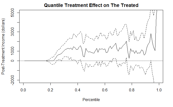
Figure 2: Quantile effect plot on the treated from the DSM algorithm
Refer to caption

8 Discussion

We have developed multiply robust matching estimators for general causal estimands. This framework offers a new “metric” to summarize the differential roles of different covariates and also serves as a powerful dimensional reduction tool in high-dimensional confounding. The improved robustness comes from multiple model specifications for the propensity score and prognostic score. The proposed DSM estimators thus provide multiple protections to model misspecification and therefore is an attractive alternative to existing weighting estimators.

Several issues are worth discussing. As with PSM, although the matching variables are well balanced, individual covariates may not for a given application. In this case, if the researchers know important confounders based on substantive knowledge, they can augment the double score by adding those confounders to ensure balance for these confounders; however, adding too many variables will results in potential bias as demonstrated in our simulation. Alternatively, one can use regression adjustment for the matched sample Abadie and Spiess 2016, which can remove remaining confounding biases. We focus on a binary treatment. Yang et al. 2016 has developed the generalized propensity score matching for estimating the treatment effects for more then two treatments. Instead of creating a matched set to estimate the treatment contrast directly, Yang et al. 2016 proposed to create matched sets to estimate potential outcome means separately. This approach allows matching based on one scalar function, namely the generalized propensity score at a given treatment level, one at a time. It is also of interest to extend our DSM algorithm to more than two treatment comparison. It is important to highlight that as for all existing matching methods, the DSM method cannot account for unmeasured confounding. Following Rosenbaum and Rubin 1983a and Robins et al. 2000, we will develop sensitivity analyses to no unmeasured confounding in the matching framework.

Acknowledgment

We are grateful to Alberto Abadie for providing comments. Yang is partially supported by the National Science Foundation grant DMS 1811245, National Cancer Institute grant P01 CA142538, National Institute on Aging grant 1R01AG066883, and National Institute of Environmental Health Science grant 1R01ES031651.

References

  • (1)
  • Abadie and Imbens (2006) Abadie, A. and Imbens, G. W. (2006). Large sample properties of matching estimators for average treatment effects, Econometrica 74: 235–267.
  • Abadie and Imbens (2008) Abadie, A. and Imbens, G. W. (2008). On the failure of the bootstrap for matching estimators, Econometrica 76: 1537–1557.
  • Abadie and Imbens (2011) Abadie, A. and Imbens, G. W. (2011). Bias-corrected matching estimators for average treatment effects, Journal of Business & Economic Statistics 29: 1–11.
  • Abadie and Imbens (2012) Abadie, A. and Imbens, G. W. (2012). A martingale representation for matching estimators, J. Am. Stat. Assoc. 107: 833–843.
  • Abadie and Imbens (2016) Abadie, A. and Imbens, G. W. (2016). Matching on the estimated propensity score, Econometrica 84: 781–807.
  • Abadie and Spiess (2016) Abadie, A. and Spiess, J. (2016). Robust post-matching inference, Unpublished Paper. MIT and Harvard University. Retrieved from https://editorialexpress. com/cgi-bin/conference/down load.
  • Andreou and Werker (2012) Andreou, E. and Werker, B. J. (2012). An alternative asymptotic analysis of residual-based statistics, Rev. Econ. Stat. 94: 88–99.
  • Antonelli et al. (2018) Antonelli, J., Cefalu, M., Palmer, N. and Agniel, D. (2018). Doubly robust matching estimators for high dimensional confounding adjustment, Biometrics 74: 1171–1179.
  • Bang and Robins (2005) Bang, H. and Robins, J. M. (2005). Doubly robust estimation in missing data and causal inference models, Biometrics 61: 962–973.
  • Bickel et al. (1993) Bickel, P. J., Klaassen, C., Ritov, Y. and Wellner, J. (1993). Efficient and Adaptive Inference in Semiparametric Models, Johns Hopkins University Press, Baltimore.
  • Billingsley (1995) Billingsley, P. (1995). Probability and Measure, 3 edn, Wiley: New York.
  • Chen and Shao (2000) Chen, J. and Shao, J. (2000). Nearest neighbor imputation for survey data, J. Offic. Stat. 16: 113–131.
  • Chen and Shao (2001) Chen, J. and Shao, J. (2001). Jackknife variance estimation for nearest-neighbor imputation, J. Am. Stat. Assoc. 96: 260–269.
  • Chen and Haziza (2017a) Chen, S. and Haziza, D. (2017a). Multiply robust imputation procedures for the treatment of item nonresponse in surveys, Biometrika 104: 439–453.
  • Chen and Haziza (2017b) Chen, S. and Haziza, D. (2017b). Multiply robust nonparametric multiple imputation for the treatment of missing data, Stat. Sin 29: 2035–2053.
  • Chen (2007) Chen, X. (2007). Large sample sieve estimation of semi-nonparametric models, Handbook of Econometrics 6: 5549–5632.
  • Chiang and Huang (2012) Chiang, C.-T. and Huang, M.-Y. (2012). New estimation and inference procedures for a single-index conditional distribution model, Journal of Multivariate Analysis 111: 271–285.
  • Dehejia and Wahba (1999) Dehejia, R. H. and Wahba, S. (1999). Causal effects in nonexperimental studies: Reevaluating the evaluation of training programs, J. Am. Stat. Assoc. 94: 1053–1062.
  • Dehejia and Wahba (2002) Dehejia, R. H. and Wahba, S. (2002). Propensity score matching methods for non-experimental causal studies, Rev. Econ. Stat. 84: 151–161.
  • Efron (1979) Efron, B. (1979). Bootstrap methods: another look at the jackknife, Annals of Statistics 7: 1–26.
  • Firpo (2007) Firpo, S. (2007). Efficient semiparametric estimation of quantile treatment effects, Econometrica 75: 259–276.
  • Ford (1983) Ford, B. L. (1983). An overview of hot-deck procedures, Incomplete data in sample surveys 2(Part IV): 185–207.
  • Francisco and Fuller (1991) Francisco, C. A. and Fuller, W. A. (1991). Quantile estimation with a complex survey design, Annals of Statistics 19: 454–469.
  • Frölich (2004) Frölich, M. (2004). Finite-sample properties of propensity-score matching and weighting estimators, Rev. Econ. Stat. 86: 77–90.
  • Guo and Fraser (2014) Guo, S. and Fraser, M. W. (2014). Propensity Score Analysis: Statistical Methods and Applications, Vol. 11, Thousand Oaks, CA: SAGE.
  • Han (2014) Han, P. (2014). Multiply robust estimation in regression analysis with missing data, J. Am. Stat. Assoc. 109(507): 1159–1173.
  • Han and Wang (2013) Han, P. and Wang, L. (2013). Estimation with missing data: beyond double robustness, Biometrika 100: 417–430.
  • Hansen (2008) Hansen, B. B. (2008). The prognostic analogue of the propensity score, Biometrika 95: 481–488.
  • Heckman et al. (1997a) Heckman, J. J., Ichimura, H. and Todd, P. E. (1997a). Matching as an econometric evaluation estimator: Evidence from evaluating a job training programme, The Review of Economic Studies 64: 605–654.
  • Heckman et al. (1997b) Heckman, J. J., Ichimura, H. and Todd, P. E. (1997b). Matching as an econometric evaluation estimator: Evidence from evaluating a job training programme, The Review of Economic Studies 64: 605–654.
  • Hernán et al. (2001) Hernán, M. A., Brumback, B. and Robins, J. M. (2001). Marginal structural models to estimate the joint causal effect of nonrandomized treatments, J. Am. Stat. Assoc. 96: 440–448.
  • Imbens (2004) Imbens, G. W. (2004). Nonparametric estimation of average treatment effects under exogeneity: A review, Rev. Econ. Stat. 86: 4–29.
  • Imbens and Rubin (2015) Imbens, G. W. and Rubin, D. B. (2015). Causal Inference in Statistics, Social, and Biomedical Sciences, Cambridge University Press, Cambridge UK.
  • Kang and Schafer (2007) Kang, J. D. and Schafer, J. L. (2007). Demystifying double robustness: A comparison of alternative strategies for estimating a population mean from incomplete data, Statistical Science 22: 523–539.
  • Kumamaru et al. (2016) Kumamaru, H., Schneeweiss, S., Glynn, R. J., Setoguchi, S. and Gagne, J. J. (2016). Dimension reduction and shrinkage methods for high dimensional disease risk scores in historical data, Emerging Themes in Epidemiology 13: Article 5.
  • LaLonde (1986) LaLonde, R. J. (1986). Evaluating the econometric evaluations of training programs with experimental data, The American Economic Review 76: 604–620.
  • Le Cam and Yang (1990) Le Cam, L. and Yang, G. L. (1990). Asymptotics in Statistics: Some Basic Concepts, Springer: Berlin.
  • Leacy and Stuart (2014) Leacy, F. P. and Stuart, E. A. (2014). On the joint use of propensity and prognostic scores in estimation of the average treatment effect on the treated: a simulation study, Stat. Med. 33: 3488–3508.
  • Little and Rubin (2002) Little, R. J. and Rubin, D. B. (2002). Statistical Analysis with Missing Data, Wiley, Hoboken.
  • Lunceford and Davidian (2004) Lunceford, J. K. and Davidian, M. (2004). Stratification and weighting via the propensity score in estimation of causal treatment effects: a comparative study, Stat. Med. 23: 2937–2960.
  • Otsu and Rai (2017) Otsu, T. and Rai, Y. (2017). Bootstrap inference of matching estimators for average treatment effects, J. Am. Stat. Assoc. 112: 1720–1732.
  • Robins et al. (2000) Robins, J. M., Rotnitzky, A. and Scharfstein, D. O. (2000). Sensitivity analysis for selection bias and unmeasured confounding in missing data and causal inference models, Statistical Models in Epidemiology, the Environment, and Clinical Trials, Springer, New York: Springer, pp. 1–94.
  • Rosenbaum (1989) Rosenbaum, P. R. (1989). Optimal matching for observational studies, J. Am. Stat. Assoc. 84: 1024–1032.
  • Rosenbaum and Rubin (1983a) Rosenbaum, P. R. and Rubin, D. B. (1983a). Assessing sensitivity to an unobserved binary covariate in an observational study with binary outcome, J. R. Stat. Soc. Ser. B Stat. Methodol. 45: 212–218.
  • Rosenbaum and Rubin (1983b) Rosenbaum, P. R. and Rubin, D. B. (1983b). The central role of the propensity score in observational studies for causal effects, Biometrika 70: 41–55.
  • Rubin (1986) Rubin, D. B. (1986). Statistical matching using file concatenation with adjusted weights and multiple imputations, Journal of Business & Economic Statistics 4: 87–94.
  • Rubin (2006) Rubin, D. B. (2006). Matched Sampling for Causal Effects, Cambridge University Press, Cambridge, England.
  • Smith and Schaubel (2015) Smith, A. R. and Schaubel, D. E. (2015). Time-dependent prognostic score matching for recurrent event analysis to evaluate a treatment assigned during follow-up, Biometrics 71: 950–959.
  • Stuart (2010) Stuart, E. A. (2010). Matching methods for causal inference: A review and a look forward, Statistical Science 25: 1–21.
  • van der Vaart (2000) van der Vaart, A. W. (2000). Asymptotic Statistics, Cambridge University Press, Cambridge, MA.
  • Wolter (2007) Wolter, K. (2007). Introduction to Variance Estimation, 2 edn, Springer, New York.
  • Wyss et al. (2015) Wyss, R., Ellis, A. R., Brookhart, M. A., Jonsson Funk, M., Girman, C. J., Simpson Jr, R. J. and Stürmer, T. (2015). Matching on the disease risk score in comparative effectiveness research of new treatments, Pharmacoepidemiology and Drug Safety 24: 951–961.
  • Wyss et al. (2017) Wyss, R., Hansen, B. B., Ellis, A. R., Gagne, J. J., Desai, R. J., Glynn, R. J. and Stürmer, T. (2017). The “dry-run” analysis: a method for evaluating risk scores for confounding control, Am. J. Epidemiol. 185: 842–852.
  • Yang and Ding (2018) Yang, S. and Ding, P. (2018). Asymptotic inference of causal effects with observational studies trimmed by the estimated propensity scores, Biometrika 105: 487–493.
  • Yang et al. (2016) Yang, S., Imbens, G. W., Cui, Z., Faries, D. E. and Kadziola, Z. (2016). Propensity score matching and subclassification in observational studies with multi-level treatments, Biometrics 72: 1055–1065.
  • Yang and Kim (2019) Yang, S. and Kim, J. K. (2019). Asymptotic theory and inference of predictive mean matching imputation using a superpopulation model framework, Scand. J. Stat. p. doi.org/10.1111/sjos.12429.
  • Zhang et al. (2012) Zhang, Z., Chen, Z., Troendle, J. F. and Zhang, J. (2012). Causal inference on quantiles with an obstetric application, Biometrics 68: 697–706.
  • Zhao (2004) Zhao, Z. (2004). Using matching to estimate treatment effects: Data requirements, matching metrics, and Monte Carlo evidence, Rev. Econ. Stat. 86: 91–107.

Supplementary Material for “Multiply robust matching estimators for average and quantile treatment effects”

Sections S1, S4, S5, and S6 present the proofs of Theorems 1, 2, 3, and 4, respectively. Section S2 compares the efficiency of PSM, PGM, and DSM. Section S3 presents Le Cam’s third lemma. Section S7 presents the extensions to the ATT and QTT. Section S8 presents a figure for the application.

S1 Proof of Theorem 1

For simplicity of the presentation, we omit the dependence of θa∗\theta_{a}^{*} for Sa​(θa∗)S_{a}(\theta_{a}^{*}) if there is no ambiguity. Following Abadie and Imbens 2011 and Abadie and Imbens 2012, under mild regularity conditions on the nonparametric estimation, we have B^n=Bn+oP​(1)\hat{B}_{n}=B_{n}+o_{P}(1). Then, τ^dsm​(θ∗)\hat{\tau}_{{\mathrm{dsm}}}(\theta^{*}) has the following asymptotic linear form:

n1/2​{τ^dsm​(θ∗)−τ}\displaystyle n^{1/2}\left\{\hat{\tau}_{{\mathrm{dsm}}}(\theta^{*})-\tau\right\} =\displaystyle= n−1/2∑i=1n{μ1(S1,i)−μ0(S0,i)−τ}\displaystyle n^{-1/2}\sum_{i=1}^{n}\left\{\mu_{1}(S_{1,i})-\mu_{0}(S_{0,i})-\tau\right\} (S3)
+n−1/2∑i=1nAi(1+M−1KS1,i){Yi−μ1(S1,i)}\displaystyle+n^{-1/2}\sum_{i=1}^{n}A_{i}\left(1+M^{-1}K_{S_{1},i}\right)\left\{Y_{i}-\mu_{1}(S_{1,i})\right\}
−n−1/2∑i=1n(1−Ai)(1+M−1KS0,i){Yi−μ0(S0,i)}+oP(1).\displaystyle-n^{-1/2}\sum_{i=1}^{n}(1-A_{i})\left(1+M^{-1}K_{S_{0},i}\right)\left\{Y_{i}-\mu_{0}(S_{0,i})\right\}+o_{P}(1).

If any model of the propensity score or prognostic score is correctly specified, by Lemma 4, we have 𝔼⁡{μ1​(S1,i)−μ0​(S0,i)}=τ{\mathbb{E}}\{\mu_{1}(S_{1,i})-\mu_{0}(S_{0,i})\}=\tau and therefore n1/2​{τ^dsm​(θ∗)−τ}n^{1/2}\left\{\hat{\tau}_{{\mathrm{dsm}}}(\theta^{*})-\tau\right\} converges to zero.

Let the three terms in (S3) be

T1​n\displaystyle T_{1n} =\displaystyle= n−1/2∑i=1n{μ1(S1,i)−μ0(S0,i)−τ},\displaystyle n^{-1/2}\sum_{i=1}^{n}\left\{\mu_{1}(S_{1,i})-\mu_{0}(S_{0,i})-\tau\right\},
T2​n\displaystyle T_{2n} =\displaystyle= n−1/2∑i=1nAi(1+M−1KS1,i){Yi−μ1(S1,i)},\displaystyle n^{-1/2}\sum_{i=1}^{n}A_{i}\left(1+M^{-1}K_{S_{1},i}\right)\left\{Y_{i}-\mu_{1}(S_{1,i})\right\},
T3​n\displaystyle T_{3n} =\displaystyle= −n−1/2∑i=1n(1−Ai)(1+M−1KS0,i){Yi−μ0(S0,i)}.\displaystyle-n^{-1/2}\sum_{i=1}^{n}(1-A_{i})\left(1+M^{-1}K_{S_{0},i}\right)\left\{Y_{i}-\mu_{0}(S_{0,i})\right\}.

We show the covariances of the three terms are zero:

cov⁡(T1​n,T2​n)\displaystyle{\mathrm{cov}}(T_{1n},T_{2n}) =\displaystyle= n−1​∑i=1n∑j=1ncov⁡[μ1​(S1,i)−μ0​(S0,i)−τ,Aj​(1+M−1​KS1,j)​{Yj−μ1​(S1,j)}]\displaystyle n^{-1}\sum_{i=1}^{n}\sum_{j=1}^{n}{\mathrm{cov}}\left[\mu_{1}(S_{1,i})-\mu_{0}(S_{0,i})-\tau,A_{j}\left(1+M^{-1}K_{S_{1},j}\right)\left\{Y_{j}-\mu_{1}(S_{1,j})\right\}\right]
=\displaystyle= n−1​∑i=1ncov⁡[μ1​(S1,i)−μ0​(S0,i)−τ,Ai​(1+M−1​KS1,i)​{Yi−μ1​(S1,i)}]\displaystyle n^{-1}\sum_{i=1}^{n}{\mathrm{cov}}\left[\mu_{1}(S_{1,i})-\mu_{0}(S_{0,i})-\tau,A_{i}\left(1+M^{-1}K_{S_{1},i}\right)\left\{Y_{i}-\mu_{1}(S_{1,i})\right\}\right]
=\displaystyle= n−1∑i=1ncov(𝔼{μ1(S1,i)−μ0(S0,i)−τ∣S1,i,S0,i},\displaystyle n^{-1}\sum_{i=1}^{n}{\mathrm{cov}}\left({\mathbb{E}}\left\{\mu_{1}(S_{1,i})-\mu_{0}(S_{0,i})-\tau\mid S_{1,i},S_{0,i}\right\},\right.
𝔼[Ai(1+M−1KS1,i){Yi−μ1(S1,i)}∣S1,i,S0,i])\displaystyle\left.{\mathbb{E}}\left[A_{i}\left(1+M^{-1}K_{S_{1},i}\right)\left\{Y_{i}-\mu_{1}(S_{1,i})\right\}\mid S_{1,i},S_{0,i}\right]\right)
+n−1∑i=1n𝔼(cov{μ1(S1,i)−μ0(S0,i)−τ∣S1,i,S0,i,\displaystyle+n^{-1}\sum_{i=1}^{n}{\mathbb{E}}\left({\mathrm{cov}}\left\{\mu_{1}(S_{1,i})-\mu_{0}(S_{0,i})-\tau\mid S_{1,i},S_{0,i},\right.\right.
Ai(1+M−1KS1,i){Yi−μ1(S1,i)}∣S1,i,S0,i})\displaystyle\left.\left.A_{i}\left(1+M^{-1}K_{S_{1},i}\right)\left\{Y_{i}-\mu_{1}(S_{1,i})\right\}\mid S_{1,i},S_{0,i}\right\}\right)
=\displaystyle= 0,\displaystyle 0,

similarly, cov⁡(T1​n,T3​n)=0{\mathrm{cov}}(T_{1n},T_{3n})=0, and by construction, cov⁡(T2​n,T3​n)=0{\mathrm{cov}}(T_{2n},T_{3n})=0. Thus, the asymptotic variance of n1/2​{τ^dsm​(θ∗)−τ}n^{1/2}\left\{\hat{\tau}_{{\mathrm{dsm}}}(\theta^{*})-\tau\right\} is

𝕍[n−1/2∑i=1n{μ1(S1,i)−μ0(S0,i)−τ}]\displaystyle{\mathbb{V}}\left[n^{-1/2}\sum_{i=1}^{n}\left\{\mu_{1}(S_{1,i})-\mu_{0}(S_{0,i})-\tau\right\}\right] +\displaystyle+ 𝕍[n−1/2∑i=1nAi(1+M−1KS1,i){Yi−μ1(S1,i)}]\displaystyle{\mathbb{V}}\left[n^{-1/2}\sum_{i=1}^{n}A_{i}\left(1+M^{-1}K_{S_{1},i}\right)\left\{Y_{i}-\mu_{1}(S_{1,i})\right\}\right]
+\displaystyle+ 𝕍[n−1/2∑i=1n(1−Ai)(1+M−1KS0,i){Yi−μ0(S0,i)}].\displaystyle{\mathbb{V}}\left[n^{-1/2}\sum_{i=1}^{n}(1-A_{i})\left(1+M^{-1}K_{S_{0},i}\right)\left\{Y_{i}-\mu_{0}(S_{0,i})\right\}\right].

The first term becomes 𝔼⁡[{μ1​(S1)−μ0​(S0)−τ}2].{\mathbb{E}}\left[\{\mu_{1}(S_{1})-\mu_{0}(S_{0})-\tau\}^{2}\right]. Following Abadie and Imbens 2006, the second and third term, as n→∞n\rightarrow\infty, becomes

plimn→∞​[n−1​∑i=1nAi​(1+M−1​KS1,i)2​𝕍​(Yi∣S1,i)]\displaystyle{\mathrm{plim}}_{n\rightarrow\infty}\left[n^{-1}\sum_{i=1}^{n}A_{i}\left(1+M^{-1}K_{S_{1},i}\right)^{2}{\mathbb{V}}(Y_{i}\mid S_{1,i})\right]
+plimn→∞​[n−1​∑i=1n(1−Ai)​(1+M−1​KS0,i)2​𝕍​(Yi∣S0,i)]\displaystyle+{\mathrm{plim}}_{n\rightarrow\infty}\left[n^{-1}\sum_{i=1}^{n}(1-A_{i})\left(1+M^{-1}K_{S_{0},i}\right)^{2}{\mathbb{V}}(Y_{i}\mid S_{0,i})\right]
=\displaystyle= 𝔼⁡(σ12​(S1)​[1e⁡(S1)+12​M​{1e⁡(S1)−e⁡(S1)}])\displaystyle{\mathbb{E}}\left(\sigma_{1}^{2}(S_{1})\left[\frac{1}{e(S_{1})}+\frac{1}{2M}\left\{\frac{1}{e(S_{1})}-e(S_{1})\right\}\right]\right)
+𝔼⁡(σ02​(S0)​[11−e⁡(S0)+12​M​{11−e⁡(S0)−1+e⁡(S0)}]).\displaystyle+{\mathbb{E}}\left(\sigma_{0}^{2}(S_{0})\left[\frac{1}{1-e(S_{0})}+\frac{1}{2M}\left\{\frac{1}{1-e(S_{0})}-1+e(S_{0})\right\}\right]\right).

S2 Comparison of PSM, PGM, and DSM

We compare the asymptotic variances of the PSM, PGM, and DSM estimators of the ATE. To simplify the discussion, we assume one working model e⁡(X,α)e(X;\alpha) for the propensity score and one working model Ψ⁡(X,β)={Ψ0​(X,β0),Ψ1​(X,β1)}\Psi(X;\beta)=\{\Psi_{0}(X;\beta_{0}),\Psi_{1}(X;\beta_{1})\} for the prognostic score. In fact, the derivation for the DSM estimator in Section S1 applies to the PSM estimator and the PGM estimator by replacing Sa=Sa​(θa∗)={e⁡(X,α∗),Ψa​(X,βa∗)}S_{a}=S_{a}(\theta_{a}^{*})=\{e(X;\alpha^{*}),\Psi_{a}(X;\beta_{a}^{*})\} (a=0,1a=0,1) with e⁡(X,α∗)e(X;\alpha^{*}) and Ψa​(X,β∗)\Psi_{a}(X;\beta^{*}), respectively.

If the prognostic score model is correctly specified, we have Ψa​(X,βa∗)=Ψa​(X)\Psi_{a}(X;\beta_{a}^{*})=\Psi_{a}(X) and therefore

μa(Sa)=𝔼{Y(a)∣Sa}=𝔼{Y(a)∣e(X;α∗),Ψa(X)}=𝔼{Y(a)∣X}=μa(X),\mu_{a}(S_{a})={\mathbb{E}}\{Y(a)\mid S_{a}\}={\mathbb{E}}\{Y(a)\mid e(X;\alpha^{*}),\Psi_{a}(X)\}={\mathbb{E}}\{Y(a)\mid X\}=\mu_{a}(X), (S4)

for a=0,1a=0,1. Then, for the DSM estimator, VτV_{\tau} in (10) becomes

Vτ,dsm=𝔼⁡[{μ1​(X)−μ0​(X)−τ}2]+𝔼⁡(σ12​(X)​[1e⁡(S1)+12​M​{1e⁡(S1)−e⁡(S1)}])+𝔼⁡(σ02​(X)​[11−e⁡(S0)+12​M​{11−e⁡(S0)−1+e⁡(S0)}]).V_{\tau,{\mathrm{dsm}}}={\mathbb{E}}\left[\{\mu_{1}(X)-\mu_{0}(X)-\tau\}^{2}\right]+{\mathbb{E}}\left(\sigma_{1}^{2}(X)\left[\frac{1}{e(S_{1})}+\frac{1}{2M}\left\{\frac{1}{e(S_{1})}-e(S_{1})\right\}\right]\right)\\ +{\mathbb{E}}\left(\sigma_{0}^{2}(X)\left[\frac{1}{1-e(S_{0})}+\frac{1}{2M}\left\{\frac{1}{1-e(S_{0})}-1+e(S_{0})\right\}\right]\right).

For the PGM estimator, it is easy to derive that the corresponding asymptotic variance is

Vτ,prog=𝔼⁡[{μ1​(X)−μ0​(X)−τ}2]+𝔼⁡{σ12​(X)​(1e​{Ψ1​(X)}+12​M​[1e​{Ψ1​(X)}−e⁡{Ψ1​(X)}])}+𝔼⁡{σ02​(X)​(11−e​{Ψ0​(X)}+12​M​[11−e​{Ψ0​(X)}−1+e⁡{Ψ0​(X)}])}.V_{\tau,{\mathrm{prog}}}={\mathbb{E}}\left[\{\mu_{1}(X)-\mu_{0}(X)-\tau\}^{2}\right]+{\mathbb{E}}\left\{\sigma_{1}^{2}(X)\left(\frac{1}{e\{\Psi_{1}(X)\}}+\frac{1}{2M}\left[\frac{1}{e\{\Psi_{1}(X)\}}-e\{\Psi_{1}(X)\}\right]\right)\right\}\\ +{\mathbb{E}}\left\{\sigma_{0}^{2}(X)\left(\frac{1}{1-e\{\Psi_{0}(X)\}}+\frac{1}{2M}\left[\frac{1}{1-e\{\Psi_{0}(X)\}}-1+e\{\Psi_{0}(X)\}\right]\right)\right\}.

By Jensen’s inequality, we have

𝔼​{1e⁡(Sa)∣Ψa​(X)}\displaystyle{\mathbb{E}}\left\{\frac{1}{e(S_{a})}\mid\Psi_{a}(X)\right\} ≥\displaystyle\geq 1𝔼⁡{e⁡(Sa)∣Ψa​(X)}=1e​{Ψa​(X)},\displaystyle\frac{1}{{\mathbb{E}}\{e(S_{a})\mid\Psi_{a}(X)\}}=\frac{1}{e\{\Psi_{a}(X)\}},
𝔼​{11−e⁡(Sa)∣Ψa​(X)}\displaystyle{\mathbb{E}}\left\{\frac{1}{1-e(S_{a})}\mid\Psi_{a}(X)\right\} ≥\displaystyle\geq 1𝔼⁡{1−e⁡(Sa)∣Ψa​(X)}=11−e​{Ψa​(X)},\displaystyle\frac{1}{{\mathbb{E}}\{1-e(S_{a})\mid\Psi_{a}(X)\}}=\frac{1}{1-e\{\Psi_{a}(X)\}},

for a=0,1a=0,1. It follows that Vτ,dsm≥Vτ,progV_{\tau,{\mathrm{dsm}}}\geq V_{\tau,{\mathrm{prog}}}.

If the propensity score model is correctly specified, we have e⁡(X,α∗)=e⁡(X)e(X;\alpha^{*})=e(X) and therefore

e(Sa)=ℙ(A=1∣Sa)=ℙ{A=1∣e(X),Ψa(X;βa∗)}=e(X).e(S_{a})={\mathbb{P}}(A=1\mid S_{a})={\mathbb{P}}\{A=1\mid e(X),\Psi_{a}(X;\beta_{a}^{*})\}=e(X). (S5)

Then, for the DSM estimator, VτV_{\tau} in (10) becomes

Vτ,dsm=𝔼⁡[{μ1​(S1)−μ0​(S0)−τ}2]+𝔼⁡(σ12​(S1)​[1e⁡(X)+12​M​{1e⁡(X)−e⁡(X)}])+𝔼⁡(σ02​(S0)​[11−e⁡(X)+12​M​{11−e⁡(X)−1+e⁡(X)}]).V_{\tau,{\mathrm{dsm}}}={\mathbb{E}}\left[\{\mu_{1}(S_{1})-\mu_{0}(S_{0})-\tau\}^{2}\right]+{\mathbb{E}}\left(\sigma_{1}^{2}(S_{1})\left[\frac{1}{e(X)}+\frac{1}{2M}\left\{\frac{1}{e(X)}-e(X)\right\}\right]\right)\\ +{\mathbb{E}}\left(\sigma_{0}^{2}(S_{0})\left[\frac{1}{1-e(X)}+\frac{1}{2M}\left\{\frac{1}{1-e(X)}-1+e(X)\right\}\right]\right).

For the PSM estimator, it is easy to derive that the corresponding asymptotic variance is

Vτ,psm=𝔼([μ1{e(X)}−μ0{e(X)}−τ]2)+𝔼(σ12{e(X)}[1e⁡(X)+12​M{1e⁡(X)−e(X)}])+𝔼⁡(σ02​{e⁡(X)}​[11−e⁡(X)+12​M​{11−e⁡(X)−1+e⁡(X)}]).V_{\tau,{\mathrm{psm}}}={\mathbb{E}}\left(\left[\mu_{1}\{e(X)\}-\mu_{0}\{e(X)\}-\tau\right]{}^{2}\right)+{\mathbb{E}}\left(\sigma_{1}^{2}\{e(X)\}\left[\frac{1}{e(X)}+\frac{1}{2M}\left\{\frac{1}{e(X)}-e(X)\right\}\right]\right)\\ +{\mathbb{E}}\left(\sigma_{0}^{2}\{e(X)\}\left[\frac{1}{1-e(X)}+\frac{1}{2M}\left\{\frac{1}{1-e(X)}-1+e(X)\right\}\right]\right).

To compare Vτ,dsmV_{\tau,{\mathrm{dsm}}} and Vτ,psmV_{\tau,{\mathrm{psm}}}, we decompose

Y⁡(a)=μa​{e⁡(X)}+ϵa,Sa|e⁡(X)⏟μa​(Sa)+ϵa,Y(a)=\underbrace{\mu_{a}\{e(X)\}+\epsilon_{a,S_{a}\mid e(X)}}_{\mu_{a}(S_{a})}+\epsilon_{a},

where ϵa,Sa|e⁡(X)\epsilon_{a,S_{a}\mid e(X)} and ϵa\epsilon_{a} have mean zero and satisfy that μa{e(X)}⟂⁣⟂{ϵa,Sa|e⁡(X),ϵa:a=0,1}\mu_{a}\{e(X)\}\mathbin{\mathchoice{\hbox to0.0pt{\hbox{$\displaystyle\perp$}\hss}\kern 3.46875pt{}\kern 3.46875pt\hbox{$\displaystyle\perp$}}{\hbox to0.0pt{\hbox{$\textstyle\perp$}\hss}\kern 3.46875pt{}\kern 3.46875pt\hbox{$\textstyle\perp$}}{\hbox to0.0pt{\hbox{$\scriptstyle\perp$}\hss}\kern 2.48856pt{}\kern 2.48856pt\hbox{$\scriptstyle\perp$}}{\hbox to0.0pt{\hbox{$\scriptscriptstyle\perp$}\hss}\kern 1.78203pt{}\kern 1.78203pt\hbox{$\scriptscriptstyle\perp$}}}\{\epsilon_{a,S_{a}\mid e(X)},\epsilon_{a}:a=0,1\} and ϵa,Sa|e⁡(X)⟂⁣⟂ϵa\epsilon_{a,S_{a}\mid e(X)}\mathbin{\mathchoice{\hbox to0.0pt{\hbox{$\displaystyle\perp$}\hss}\kern 3.46875pt{}\kern 3.46875pt\hbox{$\displaystyle\perp$}}{\hbox to0.0pt{\hbox{$\textstyle\perp$}\hss}\kern 3.46875pt{}\kern 3.46875pt\hbox{$\textstyle\perp$}}{\hbox to0.0pt{\hbox{$\scriptstyle\perp$}\hss}\kern 2.48856pt{}\kern 2.48856pt\hbox{$\scriptstyle\perp$}}{\hbox to0.0pt{\hbox{$\scriptscriptstyle\perp$}\hss}\kern 1.78203pt{}\kern 1.78203pt\hbox{$\scriptscriptstyle\perp$}}}\epsilon_{a}. With this decomposition, σa2​{e⁡(X)}=𝔼⁡{ϵa,Sa|e⁡(X)2∣e⁡(X)}+𝔼⁡(ϵa2)\sigma_{a}^{2}\{e(X)\}={\mathbb{E}}\{\epsilon_{a,S_{a}\mid e(X)}^{2}\mid e(X)\}+{\mathbb{E}}(\epsilon_{a}^{2}) and σa2​(Sa)=𝔼⁡(ϵa2)\sigma_{a}^{2}(S_{a})={\mathbb{E}}(\epsilon_{a}^{2}). Then, it follows that

Vτ,psm−Vτ,dsm\displaystyle V_{\tau,{\mathrm{psm}}}-V_{\tau,{\mathrm{dsm}}} =\displaystyle= −𝔼⁡{(ϵ1,S1|e⁡(X)−ϵ0,S0|e⁡(X))2}+𝔼⁡(ϵ1,S1|e⁡(X)2​[1e⁡(X)+12​M​{1e⁡(X)−e⁡(X)}])\displaystyle-{\mathbb{E}}\left\{\left(\epsilon_{1,S_{1}\mid e(X)}-\epsilon_{0,S_{0}\mid e(X)}\right)^{2}\right\}+{\mathbb{E}}\left(\epsilon_{1,S_{1}\mid e(X)}^{2}\left[\frac{1}{e(X)}+\frac{1}{2M}\left\{\frac{1}{e(X)}-e(X)\right\}\right]\right)
+𝔼⁡(ϵ0,S0|e⁡(X)2​[11−e⁡(X)+12​M​{11−e⁡(X)−1+e⁡(X)}])\displaystyle+{\mathbb{E}}\left(\epsilon_{0,S_{0}\mid e(X)}^{2}\left[\frac{1}{1-e(X)}+\frac{1}{2M}\left\{\frac{1}{1-e(X)}-1+e(X)\right\}\right]\right)
=\displaystyle= 2​𝔼​{ϵ1,S1|e⁡(X)​ϵ0,S0|e⁡(X)}+𝔼⁡(ϵ1,S|e⁡(X)2​[1e⁡(X)−1+12​M​{1e⁡(X)−e⁡(X)}])\displaystyle 2{\mathbb{E}}\left\{\epsilon_{1,S_{1}\mid e(X)}\epsilon_{0,S_{0}\mid e(X)}\right\}+{\mathbb{E}}\left(\epsilon_{1,S\mid e(X)}^{2}\left[\frac{1}{e(X)}-1+\frac{1}{2M}\left\{\frac{1}{e(X)}-e(X)\right\}\right]\right)
+𝔼⁡(ϵ0,S0|e⁡(X)2​[11−e⁡(X)−1+12​M​{11−e⁡(X)−1+e⁡(X)}]).\displaystyle+{\mathbb{E}}\left(\epsilon_{0,S_{0}\mid e(X)}^{2}\left[\frac{1}{1-e(X)}-1+\frac{1}{2M}\left\{\frac{1}{1-e(X)}-1+e(X)\right\}\right]\right).

The last two terms are always non-negative; however, the sign of 2​𝔼​{ϵ1,S1|e⁡(X)​ϵ0,S0|e⁡(X)}2{\mathbb{E}}\left\{\epsilon_{1,S_{1}\mid e(X)}\epsilon_{0,S_{0}\mid e(X)}\right\} and therefore that of Vτ,psm−Vτ,dsmV_{\tau,{\mathrm{psm}}}-V_{\tau,{\mathrm{dsm}}} can be either positive, negative, or zero. Therefore, for estimating τ\tau, it is not guaranteed that DSM is more efficient than PSM. For estimating μa\mu_{a}, using the similar argument as above, 2​𝔼​{ϵ1,S1|e⁡(X)​ϵ0,S0|e⁡(X)}2{\mathbb{E}}\left\{\epsilon_{1,S_{1}\mid e(X)}\epsilon_{0,S_{0}\mid e(X)}\right\} is absent, so DSM is more efficient than PSM.

S3 Le Cam’s third Lemma

Consider two sequences of probability measures (ℚ(n))n=1∞(\mathbb{Q}^{(n)})_{n=1}^{\infty} and (ℙ(n))n=1∞(\mathbb{P}^{(n)})_{n=1}^{\infty}. Assume that under ℙ(n)\mathbb{P}^{(n)}, a statistic TnT_{n} and the likelihood ratios d​ℚ(n)/d​ℙ(n){\mathrm{d}}\mathbb{Q}^{(n)}/{\mathrm{d}}\mathbb{P}^{(n)} satisfy

(Tnlog⁡(d​ℚ(n)/d​ℙ(n)))→𝒩⁡{(0−σ2/2),(τ2ccσ2)}\left(\begin{array}[]{c}T_{n}\\ \log({\mathrm{d}}\mathbb{Q}^{(n)}/{\mathrm{d}}\mathbb{P}^{(n)})\end{array}\right)\rightarrow{\mathcal{N}}\left\{\left(\begin{array}[]{c}0\\ -\sigma^{2}/2\end{array}\right),\left(\begin{array}[]{cc}\tau^{2}&c\\ c&\sigma^{2}\end{array}\right)\right\}

in distribution, as n→∞n\rightarrow\infty. Then, under ℚ(n)\mathbb{Q}^{(n)},

Tn→𝒩⁡(c,τ2)T_{n}\rightarrow{\mathcal{N}}(c,\tau^{2})

in distribution, as n→∞n\rightarrow\infty. See Le Cam and Yang 1990, Bickel et al. 1993, and van der Vaart 2000 for textbook discussions.

S4 Proof of Theorem 2

We follow the technique in Andreou and Werker 2012 and Abadie and Imbens 2016. In Abadie and Imbens 2016, the PSM estimators rely on the nuisance parameter estimator under a correct specification of the propensity score model. In our setting, the nuisance parameters include both parameters in the propensity score model and the prognostic score model, and require only one of the models to be correctly specified. Without loss of generality, we assume one working model e⁡(X,α)e(X;\alpha) for the propensity score and one working model Ψ⁡(X,β)={Ψ0​(X,β0),Ψ1​(X,β1)}\Psi(X;\beta)=\{\Psi_{0}(X;\beta_{0}),\Psi_{1}(X;\beta_{1})\} for the prognostic score. The proof for the case with more than two working models for each score is similar at the expense of heavier notation. Let ℙ{\mathbb{P}} be the distribution of {(Ai,Xi,Yi):\{(A_{i},X_{i},Y_{i}): i=1,…,n}i=1,\ldots,n\}. Consider ℙ=ℙθ∗{\mathbb{P}}={\mathbb{P}}^{\theta^{*}} to be indexed by θ∗=(α∗T,β0∗T,β1∗T)T\theta^{*}=(\alpha^{*\mathrm{\scriptscriptstyle T}},\beta_{0}^{*\mathrm{\scriptscriptstyle T}},\beta_{1}^{*\mathrm{\scriptscriptstyle T}})^{\mathrm{\scriptscriptstyle T}}, which satisfies

𝔼⁡{U⁡(A,X,Y,θ∗)}=𝔼⁡{(U1​(A,X,α∗)U2​(A,X,Y,β0∗)U3​(A,X,Y,β1∗))}=0.{\mathbb{E}}\{U(A,X,Y;\theta^{*})\}={\mathbb{E}}\left\{\left(\begin{array}[]{c}U_{1}(A,X;\alpha^{*})\\ U_{2}(A,X,Y;\beta_{0}^{*})\\ U_{3}(A,X,Y;\beta_{1}^{*})\end{array}\right)\right\}=0. (S6)

We invoke standard regularity conditions on Z-estimation (van der Vaart 2000) as follows.

Assumption S1

(i) Under ℙθ∗{\mathbb{P}}^{\theta^{*}}, 𝒰n​(θ∗)→𝒩⁡(0,ΣU){\mathcal{U}}_{n}(\theta^{*})\rightarrow{\mathcal{N}}(0,\Sigma_{U}) in distribution, as n→∞n\rightarrow\infty, where ΣU=𝔼{U(A,X,Y;θ∗)\Sigma_{U}={\mathbb{E}}\{U(A,X,Y;\theta^{*}) U(A,X,Y;θ∗)T}U(A,X,Y;\theta^{*})^{\mathrm{\scriptscriptstyle T}}\}; (ii) Γθ=𝔼⁡{∂U⁡(A,X,Y,θ)/∂θT}\Gamma_{\theta}={\mathbb{E}}\{\partial U(A,X,Y;\theta)/\partial\theta^{\mathrm{\scriptscriptstyle T}}\} is nonsingular around θ∗\theta^{*}; and (iii) for any vector of constant hh, exp⁡{n1/2​hT​Γθ∗​ΣU−1​𝒰n​(θ∗)}\exp\{n^{1/2}h^{\mathrm{\scriptscriptstyle T}}\Gamma_{\theta^{*}}\Sigma_{U}^{-1}{\mathcal{U}}_{n}(\theta^{*})\} is uniformly integrable.

Under Assumption S1,

n1/2​(θ^−θ∗)=−Γθ∗−1​𝒰n​(θ∗)+oP​(1)→𝒩⁡(0,Σθ∗),n^{1/2}(\hat{\theta}-\theta^{*})=-\Gamma_{\theta^{*}}^{-1}{\mathcal{U}}_{n}(\theta^{*})+o_{P}(1)\rightarrow{\mathcal{N}}(0,\Sigma_{\theta^{*}}), (S7)

in distribution, as n→∞n\rightarrow\infty, where Σθ∗=Γθ∗−1​ΣU​(Γθ∗−1)T\Sigma_{\theta^{*}}=\Gamma_{\theta^{*}}^{-1}\Sigma_{U}(\Gamma_{\theta^{*}}^{-1})^{\mathrm{\scriptscriptstyle T}}.

To derive the large sample distribution of τ^dsm​(θ^)\hat{\tau}_{{\mathrm{dsm}}}(\hat{\theta}), following Abadie and Imbens 2016, we impose the following regularity conditions.

Assumption S2

There exists a neighborhood of θ∗,\theta^{*}, such that for any θ\theta in this region, the following conditions hold: for a=0,1a=0,1, (i) the matching variable Sa​(θ)S_{a}(\theta) has a compact and convex support 𝒮\mathcal{S}, with a continuous density bounded and bounded away from zero; (ii) μa​{Sa​(θ)}\mu_{a}\{S_{a}(\theta)\} and σa2​{Sa​(θ)}\sigma_{a}^{2}\{S_{a}(\theta)\} satisfy the Lipschitz continuity condition; and (iii) there exists δ>0\delta>0 such that 𝔼⁡{|Y⁡(a)|2+δ∣Sa​(θ)}{\mathbb{E}}\left\{|Y(a)|^{2+\delta}\mid S_{a}(\theta)\right\} is uniformly bounded for any Sa​(θ)∈𝒮.S_{a}(\theta)\in\mathcal{S}.

Following Andreou and Werker 2012, because we consider a semiparametric model for θ∗\theta^{*}, to invoke the Le Cam’s lemma, we specify an auxiliary parametric model ℙθn{\mathbb{P}}^{\theta_{n}} defined locally though θ∗\theta^{*}, θn=θ∗+n−1/2h\theta_{n}=\theta^{*}+n^{-1/2}h, with a density

exp⁡{n1/2​(θn−θ∗)T​Γθ∗​ΣU−1​𝒰n​(θ∗)−2−1​n​(θn−θ∗)T​Σθ∗−1​(θn−θ∗)}𝔼⁡[exp⁡{n1/2​(θn−θ∗)T​Γθ∗​ΣU−1​𝒰n​(θ∗)−2−1​n​(θn−θ∗)T​Σθ∗−1​(θn−θ∗)}].\frac{\exp\left\{n^{1/2}(\theta_{n}-\theta^{*})^{\mathrm{\scriptscriptstyle T}}\Gamma_{\theta^{*}}\Sigma_{U}^{-1}{\mathcal{U}}_{n}(\theta^{*})-2^{-1}n(\theta_{n}-\theta^{*})^{\mathrm{\scriptscriptstyle T}}\Sigma_{\theta^{*}}^{-1}(\theta_{n}-\theta^{*})\right\}}{{\mathbb{E}}\left[\exp\left\{n^{1/2}(\theta_{n}-\theta^{*})^{\mathrm{\scriptscriptstyle T}}\Gamma_{\theta^{*}}\Sigma_{U}^{-1}{\mathcal{U}}_{n}(\theta^{*})-2^{-1}n(\theta_{n}-\theta^{*})^{\mathrm{\scriptscriptstyle T}}\Sigma_{\theta^{*}}^{-1}(\theta_{n}-\theta^{*})\right\}\right]}. (S8)

By Assumption S1 (iii), exp⁡{n1/2​(θn−θ∗)T​Γθ∗​ΣU−1​𝒰n​(θ∗)}\exp\{n^{1/2}(\theta_{n}-\theta^{*})^{\mathrm{\scriptscriptstyle T}}\Gamma_{\theta^{*}}\Sigma_{U}^{-1}{\mathcal{U}}_{n}(\theta^{*})\} is uniformly integrable, and thus model (S8) is uniformly locally asymptotically normal. Because under ℙθ∗{\mathbb{P}}^{\theta^{*}}, 𝒰n​(θ∗)→𝒩⁡(0,ΣU){\mathcal{U}}_{n}(\theta^{*})\rightarrow{\mathcal{N}}(0,\Sigma_{U}) in distribution, the normalizing constant in the denominator converges to one as n→∞n\rightarrow\infty. The Fisher information under the parametric model (S8) is n​Σθ∗−1.n\Sigma_{\theta^{*}}^{-1}. Therefore, θ^\hat{\theta} is efficient under model (S8).

Now consider (Ai,Xi,Yi)(A_{i},X_{i},Y_{i}), for i=1,…,ni=1,\ldots,n, with the local shift ℙθn{\mathbb{P}}^{\theta_{n}} (Bickel et al. 1993). Under model (S8), the likelihood ratio under ℙθn{\mathbb{P}}^{\theta_{n}} is

log⁡(d​ℙθ∗/d​ℙθn)\displaystyle\log({\mathrm{d}}{\mathbb{P}}^{\theta^{*}}/{\mathrm{d}}{\mathbb{P}}^{\theta_{n}}) =\displaystyle= −hT​Γθ∗​ΣU−1​𝒰n​(θ∗)+12​hT​Σθ∗−1​h+op​(1)\displaystyle-h^{\mathrm{\scriptscriptstyle T}}\Gamma_{\theta^{*}}\Sigma_{U}^{-1}{\mathcal{U}}_{n}(\theta^{*})+\frac{1}{2}h^{\mathrm{\scriptscriptstyle T}}\Sigma_{\theta^{*}}^{-1}h+o_{p}(1) (S9)
=\displaystyle= −hT​Γθ∗​ΣU−1​𝒰n​(θn)−12​hT​Σθ∗−1​h+op​(1),\displaystyle-h^{\mathrm{\scriptscriptstyle T}}\Gamma_{\theta^{*}}\Sigma_{U}^{-1}{\mathcal{U}}_{n}(\theta_{n})-\frac{1}{2}h^{\mathrm{\scriptscriptstyle T}}\Sigma_{\theta^{*}}^{-1}h+o_{p}(1),

where the second equality follows by the Taylor expansion of 𝒰n​(θ∗){\mathcal{U}}_{n}(\theta^{*}) at θn\theta_{n}. Moreover, under ℙθn{\mathbb{P}}^{\theta_{n}}: 𝒰n​(θn)→𝒩⁡(0,ΣU){\mathcal{U}}_{n}(\theta_{n})\rightarrow{\mathcal{N}}(0,\Sigma_{U}) in distribution, as n→∞n\rightarrow\infty, and

n1/2​(θ^−θn)=Γθ∗−1​𝒰n​(θn)+oP​(1).n^{1/2}(\hat{\theta}-\theta_{n})=\Gamma_{\theta^{*}}^{-1}{\mathcal{U}}_{n}(\theta_{n})+o_{P}(1). (S10)

We also assume the following regularity condition.

Assumption S3

For all bounded continuous functions h⁡(A,X,Y)h(A,X,Y), the conditional expectation 𝔼θn​{h⁡(A,X,Y)}{\mathbb{E}}_{\theta_{n}}\{h(A,X,Y)\} converges in distribution to 𝔼{h(A,X,Y){\mathbb{E}}\{h(A,X,Y)}\}, where 𝔼θn​(⋅){\mathbb{E}}_{\theta_{n}}(\cdot) is the expectation taken with respect to PθnP^{\theta_{n}}.

We derive the results in Theorem 2 in two steps.

In the first step, under ℙθn{\mathbb{P}}^{\theta_{n}}, we write τ=τ⁡(θn)\tau=\tau(\theta_{n}) to reflect its dependence on θn\theta_{n}; to be specific, we have

τ⁡(θn)=𝔼⁡[μ1​{S1​(θn)}−μ0​{S0​(θn)}].\tau(\theta_{n})={\mathbb{E}}\left[\mu_{1}\{S_{1}(\theta_{n})\}-\mu_{0}\{S_{0}(\theta_{n})\}\right].

We derive that under ℙθn{\mathbb{P}}^{\theta_{n}},

(n1/2​{τ^dsm​(θn)−τ⁡(θn)}n1/2​(θ^−θn)log⁡(d​ℙθ∗/d​ℙθn))→𝒩⁡{(00−12​hT​Σθ∗−1​h),(Vτγ1T​Γθ∗−1−γ1T​ΣU−1​Γθ∗​hΓθ∗−1​γ1Σθ∗−h−hT​Γθ∗​ΣU−1​γ1−hThT​Σθ∗−1​h)}\left(\begin{array}[]{c}n^{1/2}\{\hat{\tau}_{{\mathrm{dsm}}}(\theta_{n})-\tau(\theta_{n})\}\\ n^{1/2}(\hat{\theta}-\theta_{n})\\ \log({\mathrm{d}}{\mathbb{P}}^{\theta^{*}}/{\mathrm{d}}{\mathbb{P}}^{\theta_{n}})\end{array}\right)\rightarrow{\mathcal{N}}\left\{\left(\begin{array}[]{c}0\\ 0\\ -\frac{1}{2}h^{\mathrm{\scriptscriptstyle T}}\Sigma_{\theta^{*}}^{-1}h\end{array}\right),\left(\begin{array}[]{ccc}V_{\tau}&\gamma_{1}^{\mathrm{\scriptscriptstyle T}}\Gamma_{\theta^{*}}^{-1}&-\gamma_{1}^{\mathrm{\scriptscriptstyle T}}\Sigma_{U}^{-1}\Gamma_{\theta^{*}}h\\ \Gamma_{\theta^{*}}^{-1}\gamma_{1}&\Sigma_{\theta^{*}}&-h\\ -h^{\mathrm{\scriptscriptstyle T}}\Gamma_{\theta^{*}}\Sigma_{U}^{-1}\gamma_{1}&-h^{\mathrm{\scriptscriptstyle T}}&h^{\mathrm{\scriptscriptstyle T}}\Sigma_{\theta^{*}}^{-1}h\end{array}\right)\right\} (S11)

in distribution, as n→∞n\rightarrow\infty. We then express τ(θn)=τ(θ∗)+γ2T(n−1/2h)+o(n−1/2)\tau(\theta_{n})=\tau(\theta^{*})+\gamma_{2}^{\mathrm{\scriptscriptstyle T}}(n^{-1/2}h)+o(n^{-1/2}), where

γ2=∂τ⁡(θ)∂θ|θ=θ∗=𝔼⁡[∂μ1​{S1​(θ)}−μ0​{S0​(θ)}∂θ|θ=θ∗].\gamma_{2}=\left.\frac{\partial\tau(\theta)}{\partial\theta}\right|_{\theta=\theta^{*}}={\mathbb{E}}\left[\left.\frac{\partial\mu_{1}\{S_{1}(\theta)\}-\mu_{0}\{S_{0}(\theta)\}}{\partial\theta}\right|_{\theta=\theta^{*}}\right]. (S12)

By Le Cam’s third lemma, under ℙθ∗{\mathbb{P}}^{\theta^{*}},

(n1/2​{τ^dsm​(θn)−τ}n1/2​(θ^−θn))→𝒩⁡{(−γ1T​ΣU−1​Γθ∗​h−γ2T​h−h),(Vτγ1T​Γθ∗−1Γθ∗−1​γ1Σθ∗)}\left(\begin{array}[]{c}n^{1/2}\{\hat{\tau}_{{\mathrm{dsm}}}(\theta_{n})-\tau\}\\ n^{1/2}(\hat{\theta}-\theta_{n})\end{array}\right)\rightarrow{\mathcal{N}}\left\{\left(\begin{array}[]{c}-\gamma_{1}^{\mathrm{\scriptscriptstyle T}}\Sigma_{U}^{-1}\Gamma_{\theta^{*}}h-\gamma_{2}^{\mathrm{\scriptscriptstyle T}}h\\ -h\end{array}\right),\left(\begin{array}[]{cc}V_{\tau}&\gamma_{1}^{\mathrm{\scriptscriptstyle T}}\Gamma_{\theta^{*}}^{-1}\\ \Gamma_{\theta^{*}}^{-1}\gamma_{1}&\Sigma_{\theta^{*}}\end{array}\right)\right\}

in distribution, as n→∞n\rightarrow\infty. Replacing θn\theta_{n} by θ∗+n−1/2h\theta^{*}+n^{-1/2}h yields that under ℙθ∗{\mathbb{P}}^{\theta^{*}},

(n1/2{τ^dsm(θ∗+n−1/2h)−τ}n1/2​(θ^−θ∗))→𝒩⁡{(−γ1T​ΣU−1​Γθ∗​h−γ2T​h0),(Vτγ1T​Γθ∗−1Γθ∗−1​γ1Σθ∗)}\left(\begin{array}[]{c}n^{1/2}\{\hat{\tau}_{{\mathrm{dsm}}}(\theta^{*}+n^{-1/2}h)-\tau\}\\ n^{1/2}(\hat{\theta}-\theta^{*})\end{array}\right)\rightarrow{\mathcal{N}}\left\{\left(\begin{array}[]{c}-\gamma_{1}^{\mathrm{\scriptscriptstyle T}}\Sigma_{U}^{-1}\Gamma_{\theta^{*}}h-\gamma_{2}^{\mathrm{\scriptscriptstyle T}}h\\ 0\end{array}\right),\left(\begin{array}[]{cc}V_{\tau}&\gamma_{1}^{\mathrm{\scriptscriptstyle T}}\Gamma_{\theta^{*}}^{-1}\\ \Gamma_{\theta^{*}}^{-1}\gamma_{1}&\Sigma_{\theta^{*}}\end{array}\right)\right\} (S13)

in distribution, as n→∞n\rightarrow\infty.

In the second step, we provide a heuristic derivation for (S13) to obtain the approximate distribution (11). If the Normal distribution were exact, then

n1/2{τ^dsm(θ∗+n−1/2h)−τ}∣n1/2(θ^−θ∗)=h∼𝒩(−γ2Th,Vτ−γ1TΣU−1γ1).n^{1/2}\{\hat{\tau}_{{\mathrm{dsm}}}(\theta^{*}+n^{-1/2}h)-\tau\}\mid n^{1/2}(\hat{\theta}-\theta^{*})=h\sim{\mathcal{N}}\left(-\gamma_{2}^{\mathrm{\scriptscriptstyle T}}h,V_{\tau}-\gamma_{1}^{\mathrm{\scriptscriptstyle T}}\Sigma_{U}^{-1}\gamma_{1}\right). (S14)

Given that n1/2​(θ^−θ∗)=hn^{1/2}(\hat{\theta}-\theta^{*})=h, we have θ∗+n−1/2h=θ^\theta^{*}+n^{-1/2}h=\hat{\theta}, and hence τ^dsm(θ∗+n−1/2h)=τ^dsm(θ^)\hat{\tau}_{{\mathrm{dsm}}}(\theta^{*}+n^{-1/2}h)=\hat{\tau}_{{\mathrm{dsm}}}(\hat{\theta}). Marginalizing (S14) over the asymptotic distribution of n1/2​(θ^−θ∗)n^{1/2}(\hat{\theta}-\theta^{*}), we derive (11). The formal technique to derive (11) can be find in Andreou and Werker 2012 and Abadie and Imbens 2016. To avoid repetition, we omit this step.

In the following, we provide the proof to (S11) in the first step of the proof. Asymptotic normality of n1/2​{τ^dsm​(θn)−τ⁡(θn)}n^{1/2}\{\hat{\tau}_{{\mathrm{dsm}}}(\theta_{n})-\tau(\theta_{n})\} under ℙθn{\mathbb{P}}^{\theta_{n}} follows from Theorem 1 and the uniform local asymptotic normality of model (S8). Asymptotic joint normality of log⁡(d​ℙθ∗/d​ℙθn)\log({\mathrm{d}}{\mathbb{P}}^{\theta^{*}}/{\mathrm{d}}{\mathbb{P}}^{\theta_{n}}) and n1/2​(θ^−θn)n^{1/2}(\hat{\theta}-\theta_{n}) follows from (S9) and (S10). Also, n1/2​{τ^dsm​(θn)−τ⁡(θn)}=Dn​(θn)+oP​(1)n^{1/2}\{\hat{\tau}_{{\mathrm{dsm}}}(\theta_{n})-\tau(\theta_{n})\}=D_{n}(\theta_{n})+o_{P}(1), where

Dn​(θn)\displaystyle D_{n}(\theta_{n}) =\displaystyle= n−1/2∑i=1n[μ1{S1,i(θn)}−μ0{S0,i(θn)}−τ(θn)]\displaystyle n^{-1/2}\sum_{i=1}^{n}\left[\mu_{1}\{S_{1,i}(\theta_{n})\}-\mu_{0}\{S_{0,i}(\theta_{n})\}-\tau(\theta_{n})\right]
+n−1/2∑i=1nAi{1+M−1KS1​(θn),i}[Yi−μ1{S1,i(θn)}]\displaystyle+n^{-1/2}\sum_{i=1}^{n}A_{i}\left\{1+M^{-1}K_{S_{1}(\theta_{n}),i}\right\}\left[Y_{i}-\mu_{1}\{S_{1,i}(\theta_{n})\}\right]
−n−1/2∑i=1n(1−Ai){1+M−1KS0​(θn),i}[Yi−μ0{S0,i(θn)}]+oP(1).\displaystyle-n^{-1/2}\sum_{i=1}^{n}(1-A_{i})\left\{1+M^{-1}K_{S_{0}(\theta_{n}),i}\right\}\left[Y_{i}-\mu_{0}\{S_{0,i}(\theta_{n})\}\right]+o_{P}(1).

Therefore, the remaining is to show that, under ℙθn{\mathbb{P}}^{\theta_{n}}:

(Dn​(θn)𝒰n​(θn))→𝒩⁡{(00),(Vτγ1Tγ1ΣU)}\left(\begin{array}[]{c}D_{n}(\theta_{n})\\ {\mathcal{U}}_{n}(\theta_{n})\end{array}\right)\rightarrow{\mathcal{N}}\left\{\left(\begin{array}[]{c}0\\ 0\end{array}\right),\left(\begin{array}[]{cc}V_{\tau}&\gamma_{1}^{\mathrm{\scriptscriptstyle T}}\\ \gamma_{1}&\Sigma_{U}\end{array}\right)\right\} (S15)

in distribution, as n→∞n\rightarrow\infty. To prove (S15), consider the linear combination

Tn\displaystyle T_{n} =\displaystyle= c0​Dn​(θn)+cT​𝒰n​(θn)\displaystyle c_{0}D_{n}(\theta_{n})+c^{\mathrm{\scriptscriptstyle T}}{\mathcal{U}}_{n}(\theta_{n})
=\displaystyle= c0n−1/2∑i=1n[μ1{S1,i(θn)}−μ0{S0,i(θn)}−τ(θn)]\displaystyle c_{0}n^{-1/2}\sum_{i=1}^{n}\left[\mu_{1}\{S_{1,i}(\theta_{n})\}-\mu_{0}\{S_{0,i}(\theta_{n})\}-\tau(\theta_{n})\right]
+c0n−1/2∑i=1n(2Ai−1){1+M−1KSAi​(θn),i}[Yi−μAi{SAi,i(θn)}]\displaystyle+c_{0}n^{-1/2}\sum_{i=1}^{n}(2A_{i}-1)\left\{1+M^{-1}K_{S_{A_{i}}(\theta_{n}),i}\right\}\left[Y_{i}-\mu_{A_{i}}\{S_{A_{i},i}(\theta_{n})\}\right]
+c1Tn−1/2∑i=1n(∂e⁡(Xi,αn)∂αAi−e⁡(Xi,αn)e⁡(Xi,αn)​{1−e⁡(Xi,αn)})\displaystyle+c_{1}^{\mathrm{\scriptscriptstyle T}}n^{-1/2}\sum_{i=1}^{n}\left(\frac{\partial e(X_{i};\alpha_{n})}{\partial\alpha}\frac{A_{i}-e(X_{i};\alpha_{n})}{e(X_{i};\alpha_{n})\{1-e(X_{i};\alpha_{n})\}}\right)
+c2Tn−1/2∑i=1n((1−Ai)∂μ0​(Xi,β0,n)∂β0{Yi−μ0(Xi;β0,n)})\displaystyle+c_{2}^{\mathrm{\scriptscriptstyle T}}n^{-1/2}\sum_{i=1}^{n}\left((1-A_{i})\frac{\partial\mu_{0}(X_{i};\beta_{0,n})}{\partial\beta_{0}}\{Y_{i}-\mu_{0}(X_{i};\beta_{0,n})\}\right)
+c3Tn−1/2∑i=1n(Ai∂μ1​(Xi,β1,n)∂β1{Yi−μ1(Xi;β1,n)})+oP(1),\displaystyle+c_{3}^{\mathrm{\scriptscriptstyle T}}n^{-1/2}\sum_{i=1}^{n}\left(A_{i}\frac{\partial\mu_{1}(X_{i};\beta_{1,n})}{\partial\beta_{1}}\{Y_{i}-\mu_{1}(X_{i};\beta_{1,n})\}\right)+o_{P}(1),

where c=(c1T,c2T,c3T)Tc=(c_{1}^{\mathrm{\scriptscriptstyle T}},c_{2}^{\mathrm{\scriptscriptstyle T}},c_{3}^{\mathrm{\scriptscriptstyle T}})^{\mathrm{\scriptscriptstyle T}}. We analyze TnT_{n} using the martingale theory. We rewrite Tn=∑k=12​nξn,k,T_{n}=\sum_{k=1}^{2n}\xi_{n,k}, where

ξn,k={∑j=18ξn,k(j),1≤k≤n,∑j=911ξn,k(j),n+1≤k≤2​n,\xi_{n,k}=\begin{cases}\sum_{j=1}^{8}\xi_{n,k}^{(j)},&1\leq k\leq n,\\ \sum_{j=9}^{11}\xi_{n,k}^{(j)},&n+1\leq k\leq 2n,\end{cases}
ξn,k(1)\displaystyle\xi_{n,k}^{(1)} =\displaystyle= c0n−1/2[μ1{S1,k(θn)}−μ0{S0,k(θn)}−τ(θn)],\displaystyle c_{0}n^{-1/2}\left[\mu_{1}\{S_{1,k}(\theta_{n})\}-\mu_{0}\{S_{0,k}(\theta_{n})\}-\tau(\theta_{n})\right],
ξn,k(2)\displaystyle\xi_{n,k}^{(2)} =\displaystyle= c0n−1/2(2Ak−1){1+M−1KSAk​(θn),k}[μAk(Xk)−μAk{SAk,k(θn)}]\displaystyle c_{0}n^{-1/2}(2A_{k}-1)\left\{1+M^{-1}K_{S_{A_{k}}(\theta_{n}),k}\right\}\left[\mu_{A_{k}}(X_{k})-\mu_{A_{k}}\{S_{A_{k},k}(\theta_{n})\}\right]
ξn,k(3)\displaystyle\xi_{n,k}^{(3)} =\displaystyle= c1Tn−1/2(∂e⁡(Xk,αn)∂αe⁡(Xk)−e⁡(Xk,αn)e⁡(Xk,αn)​{1−e⁡(Xk,αn)}),\displaystyle c_{1}^{\mathrm{\scriptscriptstyle T}}n^{-1/2}\left(\frac{\partial e(X_{k};\alpha_{n})}{\partial\alpha}\frac{e(X_{k})-e(X_{k};\alpha_{n})}{e(X_{k};\alpha_{n})\{1-e(X_{k};\alpha_{n})\}}\right),
ξn,k(4)\displaystyle\xi_{n,k}^{(4)} =\displaystyle= c2Tn−1/2{1−e(Xk)}∂μ0​(Xk,β0,n)∂β0{μ0(Xk)−μ0(Xk;β0,n)},\displaystyle c_{2}^{\mathrm{\scriptscriptstyle T}}n^{-1/2}\{1-e(X_{k})\}\frac{\partial\mu_{0}(X_{k};\beta_{0,n})}{\partial\beta_{0}}\{\mu_{0}(X_{k})-\mu_{0}(X_{k};\beta_{0,n})\},
ξn,k(5)\displaystyle\xi_{n,k}^{(5)} =\displaystyle= −c3Tn−1/2e(Xk)∂μ1​(Xk,β1,n)∂β1{μ1(Xk)−μ1(Xk;β1,n)},\displaystyle-c_{3}^{\mathrm{\scriptscriptstyle T}}n^{-1/2}e(X_{k})\frac{\partial\mu_{1}(X_{k};\beta_{1,n})}{\partial\beta_{1}}\{\mu_{1}(X_{k})-\mu_{1}(X_{k};\beta_{1,n})\},
ξn,k(6)\displaystyle\xi_{n,k}^{(6)} =\displaystyle= c1Tn−1/2(∂e⁡(Xk,αn)∂αAk−e⁡(Xk)e⁡(Xk,αn)​{1−e⁡(Xk,αn)}),\displaystyle c_{1}^{\mathrm{\scriptscriptstyle T}}n^{-1/2}\left(\frac{\partial e(X_{k};\alpha_{n})}{\partial\alpha}\frac{A_{k}-e(X_{k})}{e(X_{k};\alpha_{n})\{1-e(X_{k};\alpha_{n})\}}\right),
ξn,k(7)\displaystyle\xi_{n,k}^{(7)} =\displaystyle= −c2Tn−1/2({Ak−e(Xk)}∂μ0​(Xk,β0,n)∂β0{μ0(Xk)−μ0(Xk;β0,n)}),\displaystyle-c_{2}^{\mathrm{\scriptscriptstyle T}}n^{-1/2}\left(\{A_{k}-e(X_{k})\}\frac{\partial\mu_{0}(X_{k};\beta_{0,n})}{\partial\beta_{0}}\{\mu_{0}(X_{k})-\mu_{0}(X_{k};\beta_{0,n})\}\right),
ξn,k(8)\displaystyle\xi_{n,k}^{(8)} =\displaystyle= c3Tn−1/2({Ak−e(Xk)}∂μ1​(Xk,β1,n)∂β1{μ1(Xk)−μ1(Xk;β1,n)}),\displaystyle c_{3}^{\mathrm{\scriptscriptstyle T}}n^{-1/2}\left(\{A_{k}-e(X_{k})\}\frac{\partial\mu_{1}(X_{k};\beta_{1,n})}{\partial\beta_{1}}\{\mu_{1}(X_{k})-\mu_{1}(X_{k};\beta_{1,n})\}\right),
ξn,k(9)\displaystyle\xi_{n,k}^{(9)} =\displaystyle= c0n−1/2(2Ak−n−1){1+M−1KSAk−n​(θn),k−n}{Yk−n−μAk−n(Xk−n)}\displaystyle c_{0}n^{-1/2}(2A_{k-n}-1)\left\{1+M^{-1}K_{S_{A_{k-n}}(\theta_{n}),k-n}\right\}\left\{Y_{k-n}-\mu_{A_{k-n}}(X_{k-n})\right\}
ξn,k(10)\displaystyle\xi_{n,k}^{(10)} =\displaystyle= c2Tn−1/2(1−Ak−n)∂μ0​(Xk−n,β0,n)∂β0{Yk−n−μ0(Xk−n)},\displaystyle c_{2}^{\mathrm{\scriptscriptstyle T}}n^{-1/2}(1-A_{k-n})\frac{\partial\mu_{0}(X_{k-n};\beta_{0,n})}{\partial\beta_{0}}\{Y_{k-n}-\mu_{0}(X_{k-n})\},
ξn,k(11)\displaystyle\xi_{n,k}^{(11)} =\displaystyle= c3Tn−1/2Ak−n∂μ1​(Xk−n,β1,n)∂β1{Yk−n−μ1(Xk−n)}.\displaystyle c_{3}^{\mathrm{\scriptscriptstyle T}}n^{-1/2}A_{k-n}\frac{\partial\mu_{1}(X_{k-n};\beta_{1,n})}{\partial\beta_{1}}\{Y_{k-n}-\mu_{1}(X_{k-n})\}.

Consider the σ\sigma-fields

ℱn,k={σ⁡(A1,…,Ak,X1,…,Xk),1≤k≤n,σ⁡(A1,…,An,X1,…,Xn,Yk−1,…,Yk−n),2​n+1≤k≤3​n.{\mathcal{F}}_{n,k}=\begin{cases}\sigma(A_{1},\ldots,A_{k},X_{1},\ldots,X_{k}),&1\leq k\leq n,\\ \sigma(A_{1},\ldots,A_{n},X_{1},\ldots,X_{n},Y_{k-1},\ldots,Y_{k-n}),&2n+1\leq k\leq 3n.\end{cases}

Then, we have {∑k=1iξn,i,ℱn,i,1≤i≤2n}\left\{\sum_{k=1}^{i}\xi_{n,i},{\mathcal{F}}_{n,i},1\leq i\leq 2n\right\} is a martingale for each n≥1n\geq 1, which follows by the following reasons:

(i)

because Sa,k​(θn)S_{a,k}(\theta_{n}) is a double balancing score,

𝔼θn(ξn,k(1)∣ℱn,k−1)=𝔼(c0n−1/2[μ1{S1,k(θn)}−μ0{S0,k(θn)}−τ(θn)]∣ℱn,k−1)=0;{\mathbb{E}}_{\theta_{n}}(\xi_{n,k}^{(1)}\mid{\mathcal{F}}_{n,k-1})={\mathbb{E}}\left(c_{0}n^{-1/2}\left[\mu_{1}\{S_{1,k}(\theta_{n})\}-\mu_{0}\{S_{0,k}(\theta_{n})\}-\tau(\theta_{n})\right]\mid{\mathcal{F}}_{n,k-1}\right)=0;
(ii)

let ℱn,k0=σ⁡{A1,…,Ak,S1​(θn),…,Sk​(θn)}{\mathcal{F}}_{n,k}^{0}=\sigma\{A_{1},\ldots,A_{k},S_{1}(\theta_{n}),\ldots,S_{k}(\theta_{n})\} for 1≤k≤n1\leq k\leq n, then

𝔼θn​(ξn,k(2)∣ℱn,k−1)\displaystyle{\mathbb{E}}_{\theta_{n}}(\xi_{n,k}^{(2)}\mid{\mathcal{F}}_{n,k-1}) =\displaystyle= 𝔼θn​{𝔼θn​(ξn,k(2)∣ℱn,k−10)∣ℱn,k−1}\displaystyle{\mathbb{E}}_{\theta_{n}}\{{\mathbb{E}}_{\theta_{n}}(\xi_{n,k}^{(2)}\mid{\mathcal{F}}_{n,k-1}^{0})\mid{\mathcal{F}}_{n,k-1}\}
=\displaystyle= c0n−1/2𝔼θn((2Ak−1){1+M−1KSAk​(θn),k}\displaystyle c_{0}n^{-1/2}{\mathbb{E}}_{\theta_{n}}\left((2A_{k}-1)\left\{1+M^{-1}K_{S_{A_{k}}(\theta_{n}),k}\right\}\right.
×𝔼θn[μAk(Xk)−μAk{SAk,k(θn)}∣ℱn,k−10]∣ℱn,k−1)\displaystyle\left.\times{\mathbb{E}}_{\theta_{n}}\left[\mu_{A_{k}}(X_{k})-\mu_{A_{k}}\{S_{A_{k},k}(\theta_{n})\}\mid{\mathcal{F}}_{n,k-1}^{0}\right]\mid{\mathcal{F}}_{n,k-1}\right)
=\displaystyle= c0n−1/2𝔼θn[(2Ak−1){1+M−1KSAk​(θn),k}×0∣ℱn,k−1]\displaystyle c_{0}n^{-1/2}{\mathbb{E}}_{\theta_{n}}\left[(2A_{k}-1)\left\{1+M^{-1}K_{S_{A_{k}}(\theta_{n}),k}\right\}\times 0\mid{\mathcal{F}}_{n,k-1}\right]
=\displaystyle= 0;\displaystyle 0;
(iii)

𝔼θn​(ξn,k(3)∣ℱn,k−1)=𝔼θn​(ξn,k(4)∣ℱn,k−1)=𝔼θn​(ξn,k(5)∣ℱn,k−1)=0\mathcal{{\mathbb{E}}}_{\theta_{n}}(\xi_{n,k}^{(3)}\mid{\mathcal{F}}_{n,k-1})={\mathbb{E}}_{\theta_{n}}(\xi_{n,k}^{(4)}\mid{\mathcal{F}}_{n,k-1})={\mathbb{E}}_{\theta_{n}}(\xi_{n,k}^{(5)}\mid{\mathcal{F}}_{n,k-1})=0 because 𝔼θn​{U⁡(θn)}=0{\mathbb{E}}_{\theta_{n}}\{U(\theta_{n})\}=0;

(iv)

by the conditioning argument,

𝔼θn(ξn,k(6)∣ℱn,k−1)=𝔼θn[c1Tn−1/2∂e⁡(Xk,αn)∂α𝔼{Ak−e(Xk)∣ℱn,k−1,Xk}e⁡(Xk,αn)​{1−e⁡(Xk,αn)}∣ℱn,k−1]=0;{\mathbb{E}}_{\theta_{n}}(\xi_{n,k}^{(6)}\mid{\mathcal{F}}_{n,k-1})={\mathbb{E}}_{\theta_{n}}\left[c_{1}^{\mathrm{\scriptscriptstyle T}}n^{-1/2}\frac{\partial e(X_{k};\alpha_{n})}{\partial\alpha}\frac{{\mathbb{E}}\left\{A_{k}-e(X_{k})\mid{\mathcal{F}}_{n,k-1},X_{k}\right\}}{e(X_{k};\alpha_{n})\{1-e(X_{k};\alpha_{n})\}}\mid{\mathcal{F}}_{n,k-1}\right]=0;
(v)

𝔼θn​(ξn,k(7)∣ℱn,k−1)=0{\mathbb{E}}_{\theta_{n}}(\xi_{n,k}^{(7)}\mid{\mathcal{F}}_{n,k-1})=0 and 𝔼θn​(ξn,k(8)∣ℱn,k−1)=0{\mathbb{E}}_{\theta_{n}}(\xi_{n,k}^{(8)}\mid{\mathcal{F}}_{n,k-1})=0 due to that fact that Ak−e⁡(Xk)A_{k}-e(X_{k}) is unbiased conditional on XkX_{k};

(vi)

𝔼θn​(ξn,k(9)∣ℱn,k−1)=0{\mathbb{E}}_{\theta_{n}}(\xi_{n,k}^{(9)}\mid{\mathcal{F}}_{n,k-1})=0 because (1−Ak−n)​{Yk−n−μ0​(Xk−n)}(1-A_{k-n})\{Y_{k-n}-\mu_{0}(X_{k-n})\} is unbiased given ℱn,k−1{\mathcal{F}}_{n,k-1};

(vii)

𝔼θn​(ξn,k(10)∣ℱn,k−1)=0{\mathbb{E}}_{\theta_{n}}(\xi_{n,k}^{(10)}\mid{\mathcal{F}}_{n,k-1})=0 because Ak−n​{Yk−n−μ1​(Xk−n)}A_{k-n}\{Y_{k-n}-\mu_{1}(X_{k-n})\} is unbiased given ℱn,k−1{\mathcal{F}}_{n,k-1}.

Therefore, we can apply the martingale central limit theorem (Billingsley 1995) to derive the limiting distribution of TnT_{n}. Under Assumption S2, we can verify the conditions for the martingale central limit theorem hold. It follows that under ℙθn{\mathbb{P}}^{\theta_{n}}, Tn→𝒩⁡(0,σ2)T_{n}\rightarrow{\mathcal{N}}(0,\sigma^{2}) in distribution, as n→∞n\rightarrow\infty, where σ2=plim​∑k=12​n𝔼θn​(ξn,k2∣ℱn,k−1)\sigma^{2}={\mathrm{plim}}\sum_{k=1}^{2n}{\mathbb{E}}_{\theta_{n}}(\xi_{n,k}^{2}\mid{\mathcal{F}}_{n,k-1}). Under Assumption S3, we thus derive the expression of σ2\sigma^{2} and specify the components in (S15) with

γ1=(γ11T,γ12T,γ13T)T,\gamma_{1}=(\gamma_{11}^{\mathrm{\scriptscriptstyle T}},\gamma_{12}^{\mathrm{\scriptscriptstyle T}},\gamma_{13}^{\mathrm{\scriptscriptstyle T}})^{\mathrm{\scriptscriptstyle T}}, (S16)
γ11\displaystyle\gamma_{11} =\displaystyle= 𝔼⁡([μ1​{S1​(θ∗)}−μ0​{S0​(θ∗)}−τ]​∂e⁡(X,α∗)∂α​A−e⁡(X,α∗)e⁡(X,α∗)​{1−e⁡(X,α∗)})\displaystyle{\mathbb{E}}\left(\left[\mu_{1}\{S_{1}(\theta^{*})\}-\mu_{0}\{S_{0}(\theta^{*})\}-\tau\right]\frac{\partial e(X;\alpha^{*})}{\partial\alpha}\frac{A-e(X;\alpha^{*})}{e(X;\alpha^{*})\{1-e(X;\alpha^{*})\}}\right)
+𝔼⁡([μ1​(X)−μ1​{S1​(θ∗)}]​∂e⁡(X,α∗)∂α​1−e⁡(X,α∗)e⁡(X,α∗)​{1−e⁡(X,α∗)})\displaystyle+{\mathbb{E}}\left(\left[\mu_{1}(X)-\mu_{1}\{S_{1}(\theta^{*})\}\right]\frac{\partial e(X;\alpha^{*})}{\partial\alpha}\frac{1-e(X;\alpha^{*})}{e(X;\alpha^{*})\{1-e(X;\alpha^{*})\}}\right)
−𝔼⁡([μ0​(X)−μ0​{S0​(θ∗)}]​∂e⁡(X,α∗)∂α​−e⁡(X,α∗)e⁡(X,α∗)​{1−e⁡(X,α∗)}),\displaystyle-{\mathbb{E}}\left(\left[\mu_{0}(X)-\mu_{0}\{S_{0}(\theta^{*})\}\right]\frac{\partial e(X;\alpha^{*})}{\partial\alpha}\frac{-e(X;\alpha^{*})}{e(X;\alpha^{*})\{1-e(X;\alpha^{*})\}}\right),
γ12\displaystyle\gamma_{12} =\displaystyle= −𝔼⁡([μ1​{S1​(θ∗)}−μ0​{S0​(θ∗)}−τ]​(1−A)​∂μ0​(X,β0∗)∂β0​{μ0​(X)−μ0​(X,β0∗)})\displaystyle-{\mathbb{E}}\left(\left[\mu_{1}\{S_{1}(\theta^{*})\}-\mu_{0}\{S_{0}(\theta^{*})\}-\tau\right](1-A)\frac{\partial\mu_{0}(X;\beta_{0}^{*})}{\partial\beta_{0}}\{\mu_{0}(X)-\mu_{0}(X;\beta_{0}^{*})\}\right)
−𝔼⁡([μ0​(X)−μ0​{S0​(θ∗)}]​∂μ0​(X,β0∗)∂β0​{μ0​(X)−μ0​(X,β0∗)})−𝔼⁡{∂μ0​(X,β0∗)∂β0​σ02​(X)},\displaystyle-{\mathbb{E}}\left(\left[\mu_{0}(X)-\mu_{0}\{S_{0}(\theta^{*})\}\right]\frac{\partial\mu_{0}(X;\beta_{0}^{*})}{\partial\beta_{0}}\{\mu_{0}(X)-\mu_{0}(X;\beta_{0}^{*})\}\right)-{\mathbb{E}}\left\{\frac{\partial\mu_{0}(X;\beta_{0}^{*})}{\partial\beta_{0}}\sigma_{0}^{2}(X)\right\},

and

γ13\displaystyle\gamma_{13} =\displaystyle= −𝔼⁡([μ1​{S1​(θ∗)}−μ0​{S0​(θ∗)}−τ]​A​∂μ1​(X,β1∗)∂β1​{μ1​(X)−μ1​(X,β1∗)})\displaystyle-{\mathbb{E}}\left(\left[\mu_{1}\{S_{1}(\theta^{*})\}-\mu_{0}\{S_{0}(\theta^{*})\}-\tau\right]A\frac{\partial\mu_{1}(X;\beta_{1}^{*})}{\partial\beta_{1}}\{\mu_{1}(X)-\mu_{1}(X;\beta_{1}^{*})\}\right)
−𝔼⁡([μ1​(X)−μ1​{S1​(θ∗)}]​∂μ1​(X,β1∗)∂β1​{μ1​(X)−μ1​(X,β1∗)})−𝔼⁡{∂μ1​(X,β1∗)∂β1​σ12​(X)}.\displaystyle-{\mathbb{E}}\left(\left[\mu_{1}(X)-\mu_{1}\{S_{1}(\theta^{*})\}\right]\frac{\partial\mu_{1}(X;\beta_{1}^{*})}{\partial\beta_{1}}\{\mu_{1}(X)-\mu_{1}(X;\beta_{1}^{*})\}\right)-{\mathbb{E}}\left\{\frac{\partial\mu_{1}(X;\beta_{1}^{*})}{\partial\beta_{1}}\sigma_{1}^{2}(X)\right\}.

S5 Proof of Theorem 3

Under Assumption 4, we can write

F^a,dsm(q^a,ξ,dsm)−Fa(qa,ξ)=F^a,dsm(qa,ξ)−Fa(qa,ξ)+fa(qa,ξ)(q^a,ξ,dsm−qa,ξ)+oP(n−1/2).\hat{F}_{a,{\mathrm{dsm}}}(\hat{q}_{a,\xi,{\mathrm{dsm}}})-F_{a}(q_{a,\xi})=\hat{F}_{a,{\mathrm{dsm}}}(q_{a,\xi})-F_{a}(q_{a,\xi})+f_{a}(q_{a,\xi})(\hat{q}_{a,\xi,{\mathrm{dsm}}}-q_{a,\xi})+o_{\mathrm{P}}(n^{-1/2}). (S17)

Then the Bahadur-type representation for q^a,ξ,dsm\hat{q}_{a,\xi,{\mathrm{dsm}}} in (15) follows.

We obtain the following decomposition

n1/2​{F^a,dsm(0)​(q)−Fa​(q)}\displaystyle n^{1/2}\left\{\hat{F}_{a,{\mathrm{dsm}}}^{(0)}(q)-F_{a}(q)\right\} =\displaystyle= n−1/2∑i=1n{𝟏(Ai=a)(1+M−1KSa,i)𝟏(Yi≤q)−Fa(q)}\displaystyle n^{-1/2}\sum_{i=1}^{n}\left\{\mathbf{1}(A_{i}=a)\left(1+M^{-1}K_{S_{a},i}\right)\mathbf{1}(Y_{i}\leq q)-F_{a}(q)\right\}
=\displaystyle= n−1/2∑i=1n𝟏(Ai=a)(1+M−1KSa,i){𝟏(Yi≤q)−Fa(q;Sa,i)}\displaystyle n^{-1/2}\sum_{i=1}^{n}\mathbf{1}(A_{i}=a)\left(1+M^{-1}K_{S_{a},i}\right)\left\{\mathbf{1}(Y_{i}\leq q)-F_{a}(q;S_{a,i})\right\}
+n−1/2∑i=1n{𝟏(Ai=a)(1+M−1KSa,i)Fa(q;Sa,i)−Fa(q)}\displaystyle+n^{-1/2}\sum_{i=1}^{n}\left\{\mathbf{1}(A_{i}=a)\left(1+M^{-1}K_{S_{a},i}\right)F_{a}(q;S_{a,i})-F_{a}(q)\right\}
=\displaystyle= n−1/2∑i=1n{Fa(q;Sa,i)−Fa(q)}\displaystyle n^{-1/2}\sum_{i=1}^{n}\left\{F_{a}(q;S_{a,i})-F_{a}(q)\right\}
+n−1/2∑i=1n𝟏(Ai=a)(1+M−1KSa,i){𝟏(Yi≤q)−Fa(q;Sa,i)}\displaystyle+n^{-1/2}\sum_{i=1}^{n}\mathbf{1}(A_{i}=a)\left(1+M^{-1}K_{S_{a},i}\right)\left\{\mathbf{1}(Y_{i}\leq q)-F_{a}(q;S_{a,i})\right\}
−n−1/2∑i=1n𝟏(Ai=1−a)M−1∑j∈𝒥Sa,i{Fa(q;Sa,i)−Fa(q;Sa,j)}\displaystyle-n^{-1/2}\sum_{i=1}^{n}\mathbf{1}(A_{i}=1-a)M^{-1}\sum_{j\in{\mathcal{J}}_{S_{a},i}}\left\{F_{a}(q;S_{a,i})-F_{a}(q;S_{a,j})\right\}

and denote

Ca,n​(q)\displaystyle C_{a,n}(q) =\displaystyle= n−1/2∑i=1n{Fa(q;Sa,i)−Fa(q)}\displaystyle n^{-1/2}\sum_{i=1}^{n}\left\{F_{a}(q;S_{a,i})-F_{a}(q)\right\}
+n−1/2∑i=1n𝟏(Ai=a)(1+M−1KSa,i){𝟏(Yi≤q)−Fa(q;Sa,i)},\displaystyle+n^{-1/2}\sum_{i=1}^{n}\mathbf{1}(A_{i}=a)\left(1+M^{-1}K_{S_{a},i}\right)\left\{\mathbf{1}(Y_{i}\leq q)-F_{a}(q;S_{a,i})\right\},
Ba,n​(q)\displaystyle B_{a,n}(q) =\displaystyle= −n−1/2∑i=1n𝟏(Ai=1−a)M−1∑j∈𝒥Sa,i{Fa(q;Sa,i)−Fa(q;Sa,j)}.\displaystyle-n^{-1/2}\sum_{i=1}^{n}\mathbf{1}(A_{i}=1-a)M^{-1}\sum_{j\in{\mathcal{J}}_{S_{a},i}}\left\{F_{a}(q;S_{a,i})-F_{a}(q;S_{a,j})\right\}. (S18)

Because of (1) and (2), 𝔼⁡{Fa​(q,Sa,i)}=Fa​(q){\mathbb{E}}\{F_{a}(q;S_{a,i})\}=F_{a}(q), so 𝔼​{Ca,n​(q)}=0{\mathbb{E}}\{C_{a,n}(q)\}=0. The difference Fa​(q,Sa,i)−Fa​(q,Sa,j)F_{a}(q;S_{a,i})-F_{a}(q;S_{a,j}) in (S18) accounts for the matching discrepancy, and therefore Ba,n​(q)B_{a,n}(q) contributes to the asymptotic bias of the matching estimator. To correct for the bias due to matching discrepancy, let F^a​(q,S)\hat{F}_{a}(q;S) be a nonparametric estimator of Fa​(q,S)F_{a}(q;S), for a=0,1a=0,1. We propose a de-biasing DSM estimator F^a,dsm​(q)\hat{F}_{a,{\mathrm{dsm}}}(q) of Fa​(q)F_{a}(q) in (13).

Therefore, by the Bahadur-type representation for q^a,ξ,dsm\hat{q}_{a,\xi,{\mathrm{dsm}}}, we have

n1/2​{Δ^ξ,dsm​(θ∗)−Δξ}\displaystyle n^{1/2}\left\{\hat{\Delta}_{\xi,{\mathrm{dsm}}}(\theta^{*})-\Delta_{\xi}\right\} =\displaystyle= n1/2​{−F^1,dsm​(q1,ξ)f1​(q1,ξ)+F^0,dsm​(q0,ξ)f0​(q0,ξ)−Δξ}+oP​(1)\displaystyle n^{1/2}\left\{-\frac{\hat{F}_{1,{\mathrm{dsm}}}(q_{1,\xi})}{f_{1}(q_{1,\xi})}+\frac{\hat{F}_{0,{\mathrm{dsm}}}(q_{0,\xi})}{f_{0}(q_{0,\xi})}-\Delta_{\xi}\right\}+o_{P}(1)
=\displaystyle= n−1/2∑i=1n{−F1​(q1,ξ,S1,i)f1​(q1,ξ)+F0​(q0,ξ,S0,i)f0​(q0,ξ)−Δξ}\displaystyle n^{-1/2}\sum_{i=1}^{n}\left\{-\frac{F_{1}(q_{1,\xi};S_{1,i})}{f_{1}(q_{1,\xi})}+\frac{F_{0}(q_{0,\xi};S_{0,i})}{f_{0}(q_{0,\xi})}-\Delta_{\xi}\right\}
−n−1/2∑i=1n(2Ai−1){1+M−1KSAi,i}{𝟏​(Yi≤qAi,ξ)−FAi​(qAi,ξ,SAi,i)fAi​(qAi,ξ)}+oP(1).\displaystyle-n^{-1/2}\sum_{i=1}^{n}(2A_{i}-1)\left\{1+M^{-1}K_{S_{A_{i}},i}\right\}\left\{\frac{\mathbf{1}(Y_{i}\leq q_{A_{i},\xi})-F_{A_{i}}(q_{A_{i},\xi};S_{A_{i},i})}{f_{A_{i}}(q_{A_{i},\xi})}\right\}+o_{P}(1).

Following a similar derivation in the proof for Theorem 1, the asymptotic variance of n1/2​{Δ^ξ,dsm​(θ∗)−Δξ}n^{1/2}\left\{\hat{\Delta}_{\xi,{\mathrm{dsm}}}(\theta^{*})-\Delta_{\xi}\right\} is given by

VΔ=𝔼⁡[{F1​(q1,ξ,S1)f1​(q1,ξ)−F0​(q0,ξ,S0)f0​(q0,ξ)}2]+{f1​(q1,ξ)}−2​𝔼​(F1​(q1,ξ,S1)​{1−F1​(q1,ξ,S1)}​[1e⁡(S1)+12​M​{1e⁡(S1)−e⁡(S1)}])+{f0​(q0,ξ)}−2​𝔼​(F0​(q0,ξ,S0)​{1−F0​(q0,ξ,S0)}​[11−e⁡(S0)+12​M​{11−e⁡(S0)−1+e⁡(S0)}]).V_{\Delta}={\mathbb{E}}\left[\left\{\frac{F_{1}(q_{1,\xi};S_{1})}{f_{1}(q_{1,\xi})}-\frac{F_{0}(q_{0,\xi};S_{0})}{f_{0}(q_{0,\xi})}\right\}^{2}\right]\\ +\{f_{1}(q_{1,\xi})\}^{-2}{\mathbb{E}}\left(F_{1}(q_{1,\xi};S_{1})\{1-F_{1}(q_{1,\xi};S_{1})\}\left[\frac{1}{e(S_{1})}+\frac{1}{2M}\left\{\frac{1}{e(S_{1})}-e(S_{1})\right\}\right]\right)\\ +\{f_{0}(q_{0,\xi})\}^{-2}{\mathbb{E}}\left(F_{0}(q_{0,\xi};S_{0})\{1-F_{0}(q_{0,\xi};S_{0})\}\left[\frac{1}{1-e(S_{0})}+\frac{1}{2M}\left\{\frac{1}{1-e(S_{0})}-1+e(S_{0})\right\}\right]\right). (S19)

S6 Proof of Theorem 4

The proof of Theorem 4 is similar to that of Theorem 2. It suffices to replace n1/2​{τ^dsm​(θn)−τ}n^{1/2}\{\hat{\tau}_{{\mathrm{dsm}}}(\theta_{n})-\tau\} in (S13) by n1/2​{Δ^ξ,dsm​(θn)−Δξ}n^{1/2}\{\hat{\Delta}_{\xi,{\mathrm{dsm}}}(\theta_{n})-\Delta_{\xi}\} and derive the corresponding γ1\gamma_{1} and γ2\gamma_{2}, denoted by γ3\gamma_{3} and γ4\gamma_{4}.

Toward that end, the key is to write

q^1,ξ,dsm−q^0,ξ,dsm−Δξ​(θ∗)\displaystyle\hat{q}_{1,\xi,{\mathrm{dsm}}}-\hat{q}_{0,\xi,{\mathrm{dsm}}}-\Delta_{\xi}(\theta^{*}) =\displaystyle= −F^1,dsm​(q1,ξ)−F1​(q1,ξ)f1​(q1,ξ)+F^0,dsm​(q0,ξ)−F0​(q0,ξ)f0​(q0,ξ)+oP(n−1/2),\displaystyle-\frac{\hat{F}_{1,{\mathrm{dsm}}}(q_{1,\xi})-F_{1}(q_{1,\xi})}{f_{1}(q_{1,\xi})}+\frac{\hat{F}_{0,{\mathrm{dsm}}}(q_{0,\xi})-F_{0}(q_{0,\xi})}{f_{0}(q_{0,\xi})}+o_{P}(n^{-1/2}),

where

F^a,dsm​(qa,ξ)\displaystyle\hat{F}_{a,{\mathrm{dsm}}}(q_{a,\xi}) =\displaystyle= n−1​∑i=1n[Fa​{qa,ξ;Sa​(θ∗)}−ξ]\displaystyle n^{-1}\sum_{i=1}^{n}\left[F_{a}\{q_{a,\xi};S_{a}(\theta^{*})\}-\xi\right]
+n−1∑i=1n𝟏(Ai=a)(1+M−1KSa,i)[𝟏(Yi≤qa,ξ)−Fa{qa,ξ;Sa(θ∗)}],\displaystyle+n^{-1}\sum_{i=1}^{n}\mathbf{1}(A_{i}=a)\left(1+M^{-1}K_{S_{a},i}\right)\left[\mathbf{1}(Y_{i}\leq q_{a,\xi})-F_{a}\{q_{a,\xi};S_{a}(\theta^{*})\}\right],
Δξ​(θ∗)\displaystyle\Delta_{\xi}(\theta^{*}) =\displaystyle= 𝔼⁡[Ae⁡(X,α∗)​𝟏​(Y≤q1,ξ)−F1​{q1,ξ;S1​(θ∗)}f1​(q1,ξ)−1−A1−e⁡(X,α)​𝟏​(Y≤q0,ξ)−F0​{q0,ξ;S0​(θ∗)}f0​(q0,ξ)]\displaystyle{\mathbb{E}}\left[\frac{A}{e(X;\alpha^{*})}\frac{\mathbf{1}(Y\leq q_{1,\xi})-F_{1}\{q_{1,\xi};S_{1}(\theta^{*})\}}{f_{1}(q_{1,\xi})}-\frac{1-A}{1-e(X;\alpha)}\frac{\mathbf{1}(Y\leq q_{0,\xi})-F_{0}\{q_{0,\xi};S_{0}(\theta^{*})\}}{f_{0}(q_{0,\xi})}\right]
+𝔼⁡[F1​{q1,ξ;S1​(θ∗)}f1​(q1,ξ)−F0​{q0,ξ;S0​(θ∗)}f0​(q0,ξ)],\displaystyle+{\mathbb{E}}\left[\frac{F_{1}\{q_{1,\xi};S_{1}(\theta^{*})\}}{f_{1}(q_{1,\xi})}-\frac{F_{0}\{q_{0,\xi};S_{0}(\theta^{*})\}}{f_{0}(q_{0,\xi})}\right],

and repeat a similar analysis in Section S4 with the following changes to ξn,k(1)\xi_{n,k}^{(1)}, ξn,k(2)\xi_{n,k}^{(2)} and ξn,k(9)\xi_{n,k}^{(9)}:

ξ~n,k(1)\displaystyle\tilde{\xi}_{n,k}^{(1)} =\displaystyle= c0n−1/2[f1(q1,ξ)−1F1{q1,ξ;S1,k(θn)}−f0(q0,ξ)−1F0{q0,ξ;S0,k(θn)}−Δξ(θn)],\displaystyle c_{0}n^{-1/2}\left[f_{1}(q_{1,\xi})^{-1}F_{1}\{q_{1,\xi};S_{1,k}(\theta_{n})\}-f_{0}(q_{0,\xi})^{-1}F_{0}\{q_{0,\xi};S_{0,k}(\theta_{n})\}-\Delta_{\xi}(\theta_{n})\right],
ξ~n,k(2)\displaystyle\tilde{\xi}_{n,k}^{(2)} =\displaystyle= c0n−1/2(2Ak−1){1+M−1KSAk​(θn),k}fAk(qAk,ξ)−1[FAk(qAk,ξ;Xk)−FAk{qAk,ξ;SAk,k(θn)}],\displaystyle c_{0}n^{-1/2}(2A_{k}-1)\left\{1+M^{-1}K_{S_{A_{k}}(\theta_{n}),k}\right\}f_{A_{k}}(q_{A_{k},\xi})^{-1}\left[F_{A_{k}}(q_{A_{k},\xi};X_{k})-F_{A_{k}}\{q_{A_{k},\xi};S_{A_{k},k}(\theta_{n})\}\right],
ξ~n,k(9)\displaystyle\tilde{\xi}_{n,k}^{(9)} =\displaystyle= c0n−1/2(2Ak−n−1){1+M−1KSAk​(θn),k−n}fAk−n(qAk−n,ξ)−1\displaystyle c_{0}n^{-1/2}(2A_{k-n}-1)\left\{1+M^{-1}K_{S_{A_{k}}(\theta_{n}),k-n}\right\}f_{A_{k-n}}(q_{A_{k-n},\xi})^{-1}
×{𝟏​(Yk−n≤qAk−n,ξ)−FAk−n​(qAk−n,ξ,Xk−n)}.\displaystyle\times\left\{\mathbf{1}(Y_{k-n}\leq q_{A_{k-n},\xi})-F_{A_{k-n}}(q_{A_{k-n},\xi};X_{k-n})\right\}.

Then, we can derive

γ3T=(γ31T,γ32T,γ33T),\gamma_{3}^{\mathrm{\scriptscriptstyle T}}=(\gamma_{31}^{\mathrm{\scriptscriptstyle T}},\gamma_{32}^{\mathrm{\scriptscriptstyle T}},\gamma_{33}^{\mathrm{\scriptscriptstyle T}}), (S20)

where

γ31\displaystyle\gamma_{31} =\displaystyle= 𝔼⁡([F1​{q1,ξ;S1​(θ∗)}f1​(q1,ξ)−F0​{q0,ξ;S0​(θ∗)}f0​(q0,ξ)−Δξ]​∂e⁡(X,α∗)∂α​A−e⁡(X,α∗)e⁡(X,α∗)​{1−e⁡(X,α∗)})\displaystyle{\mathbb{E}}\left(\left[\frac{F_{1}\{q_{1,\xi};S_{1}(\theta^{*})\}}{f_{1}(q_{1,\xi})}-\frac{F_{0}\{q_{0,\xi};S_{0}(\theta^{*})\}}{f_{0}(q_{0,\xi})}-\Delta_{\xi}\right]\frac{\partial e(X;\alpha^{*})}{\partial\alpha}\frac{A-e(X;\alpha^{*})}{e(X;\alpha^{*})\{1-e(X;\alpha^{*})\}}\right)
+𝔼⁡(f1​(q1,ξ)−1​[F1​(q1,ξ,X)−F1​{q1,ξ;S1​(θ∗)}]​∂e⁡(X,α∗)∂α​1−e⁡(X,α∗)e⁡(X,α∗)​{1−e⁡(X,α∗)})\displaystyle+{\mathbb{E}}\left(f_{1}(q_{1,\xi})^{-1}\left[F_{1}(q_{1,\xi};X)-F_{1}\{q_{1,\xi};S_{1}(\theta^{*})\}\right]\frac{\partial e(X;\alpha^{*})}{\partial\alpha}\frac{1-e(X;\alpha^{*})}{e(X;\alpha^{*})\{1-e(X;\alpha^{*})\}}\right)
−𝔼⁡(f0​(q0,ξ)−1​[F0​(q0,ξ,X)−F0​{q0,ξ;S0​(θ∗)}]​∂e⁡(X,α∗)∂α​−e⁡(X,α∗)e⁡(X,α∗)​{1−e⁡(X,α∗)}),\displaystyle-{\mathbb{E}}\left(f_{0}(q_{0,\xi})^{-1}\left[F_{0}(q_{0,\xi};X)-F_{0}\{q_{0,\xi};S_{0}(\theta^{*})\}\right]\frac{\partial e(X;\alpha^{*})}{\partial\alpha}\frac{-e(X;\alpha^{*})}{e(X;\alpha^{*})\{1-e(X;\alpha^{*})\}}\right),
γ32\displaystyle\gamma_{32} =\displaystyle= −𝔼⁡([F1​{q1,ξ;S1​(θ∗)}f1​(q1,ξ)−F0​{q0,ξ;S0​(θ∗)}f0​(q0,ξ)−Δξ]​(1−A)​∂μ0​(X,β0∗)∂β0​{μ0​(X)−μ0​(X,β0∗)})\displaystyle-{\mathbb{E}}\left(\left[\frac{F_{1}\{q_{1,\xi};S_{1}(\theta^{*})\}}{f_{1}(q_{1,\xi})}-\frac{F_{0}\{q_{0,\xi};S_{0}(\theta^{*})\}}{f_{0}(q_{0,\xi})}-\Delta_{\xi}\right](1-A)\frac{\partial\mu_{0}(X;\beta_{0}^{*})}{\partial\beta_{0}}\{\mu_{0}(X)-\mu_{0}(X;\beta_{0}^{*})\}\right)
−𝔼⁡(f0​(q0,ξ)−1​[F0​(q0,ξ,X)−F0​{q0,ξ;S0​(θ∗)}]​∂μ0​(X,β0∗)∂β0​{μ0​(X)−μ0​(X,β0∗)})\displaystyle-{\mathbb{E}}\left(f_{0}(q_{0,\xi})^{-1}\left[F_{0}(q_{0,\xi};X)-F_{0}\{q_{0,\xi};S_{0}(\theta^{*})\}\right]\frac{\partial\mu_{0}(X;\beta_{0}^{*})}{\partial\beta_{0}}\{\mu_{0}(X)-\mu_{0}(X;\beta_{0}^{*})\}\right)
−𝔼{∂μ0​(X,β0∗)∂β0f0(q0,ξ)−1[I{Y(0)≤q0,ξ}−F0(q0,ξ;X)]{Y(0)−μ0(X)}},\displaystyle-{\mathbb{E}}\left\{\frac{\partial\mu_{0}(X;\beta_{0}^{*})}{\partial\beta_{0}}f_{0}(q_{0,\xi})^{-1}\left[I\{Y(0)\leq q_{0,\xi}\}-F_{0}(q_{0,\xi};X)\right]\{Y(0)-\mu_{0}(X)\}\right\},
γ33\displaystyle\gamma_{33} =\displaystyle= −𝔼⁡([F1​{q1,ξ;S1​(θ∗)}f1​(q1,ξ)−F0​{q0,ξ;S0​(θ∗)}f0​(q0,ξ)−Δξ]​A​∂μ1​(X,β1∗)∂β1​{μ1​(X)−μ1​(X,β1∗)})\displaystyle-{\mathbb{E}}\left(\left[\frac{F_{1}\{q_{1,\xi};S_{1}(\theta^{*})\}}{f_{1}(q_{1,\xi})}-\frac{F_{0}\{q_{0,\xi};S_{0}(\theta^{*})\}}{f_{0}(q_{0,\xi})}-\Delta_{\xi}\right]A\frac{\partial\mu_{1}(X;\beta_{1}^{*})}{\partial\beta_{1}}\{\mu_{1}(X)-\mu_{1}(X;\beta_{1}^{*})\}\right)
−𝔼⁡(f1​(q1,ξ)−1​[F1​(q1,ξ,X)−F1​{q1,ξ;S1​(θ∗)}]​∂μ1​(X,β1∗)∂β1​{μ1​(X)−μ1​(X,β1∗)})\displaystyle-{\mathbb{E}}\left(f_{1}(q_{1,\xi})^{-1}\left[F_{1}(q_{1,\xi};X)-F_{1}\{q_{1,\xi};S_{1}(\theta^{*})\}\right]\frac{\partial\mu_{1}(X;\beta_{1}^{*})}{\partial\beta_{1}}\{\mu_{1}(X)-\mu_{1}(X;\beta_{1}^{*})\}\right)
−𝔼{∂μ1​(X,β1∗)∂β1f1(q1,ξ)−1[𝟏{Y(1)≤q1,ξ}−F1(q1,ξ;X)]{Y(1)−μ1(X)}},\displaystyle-{\mathbb{E}}\left\{\frac{\partial\mu_{1}(X;\beta_{1}^{*})}{\partial\beta_{1}}f_{1}(q_{1,\xi})^{-1}\left[\mathbf{1}\{Y(1)\leq q_{1,\xi}\}-F_{1}(q_{1,\xi};X)\right]\{Y(1)-\mu_{1}(X)\}\right\},

and

γ4=−𝔼⁡[1f1​(q1,ξ)​∂F1​{q1,ξ;S1​(θ∗)}∂θ−1f0​(q0,ξ)​∂F0​{q0,ξ;S0​(θ∗)}∂θ].\gamma_{4}=-{\mathbb{E}}\left[\frac{1}{f_{1}(q_{1,\xi})}\frac{\partial F_{1}\{q_{1,\xi};S_{1}(\theta^{*})\}}{\partial\theta}-\frac{1}{f_{0}(q_{0,\xi})}\frac{\partial F_{0}\{q_{0,\xi};S_{0}(\theta^{*})\}}{\partial\theta}\right]. (S21)

S7 Extensions to the causal effects on the treated

In this extension, we estimate the average causal effect on the treated τATT\tau_{\mathrm{ATT}} and the quantile treatment effect on the treated ΔATT,ξ=q1,ξ|A=1−q0,ξ|A=1\Delta_{\mathrm{ATT},\xi}=q_{1,\xi\mid A=1}-q_{0,\xi\mid A=1}, where qa,ξ|A=1=infq[P{Y(a)≤q}≥ξ∣A=1]q_{a,\xi\mid A=1}=\inf_{q}[P\{Y(a)\leq q\}\geq\xi\mid A=1], a=0,1a=0,1. Here, because f⁡{Y⁡(1)∣A=1}=f⁡(Y∣A=1)f\{Y(1)\mid A=1\}=f(Y\mid A=1), the outcome distribution for the treated is identifiable. Therefore, 𝔼⁡{Y⁡(1)∣A=1}=𝔼⁡(Y∣A=1){\mathbb{E}}\{Y(1)\mid A=1\}={\mathbb{E}}(Y\mid A=1) and q1,ξ|A=1=infq{ℙ(Y≤q∣A=1)≥ξ}q_{1,\xi\mid A=1}=\inf_{q}\left\{{\mathbb{P}}(Y\leq q\mid A=1)\geq\xi\right\}.

To identify the outcome distribution for the control, Assumptions 2 and 1 can be relaxed (Heckman et al. 1997b).

Assumption S4

Y⁡(0)⟂⁣⟂A|XY(0)\mathbin{\mathchoice{\hbox to0.0pt{\hbox{$\displaystyle\perp$}\hss}\kern 3.46875pt{}\kern 3.46875pt\hbox{$\displaystyle\perp$}}{\hbox to0.0pt{\hbox{$\textstyle\perp$}\hss}\kern 3.46875pt{}\kern 3.46875pt\hbox{$\textstyle\perp$}}{\hbox to0.0pt{\hbox{$\scriptstyle\perp$}\hss}\kern 2.48856pt{}\kern 2.48856pt\hbox{$\scriptstyle\perp$}}{\hbox to0.0pt{\hbox{$\scriptscriptstyle\perp$}\hss}\kern 1.78203pt{}\kern 1.78203pt\hbox{$\scriptscriptstyle\perp$}}}A\mid X.

Assumption S5

There exists a constant cc such that e⁡(X)≤c<1e(X)\leq c<1 almost surely.

For the causal effects on the treated, the prognostic score Ψ0​(X)\Psi_{0}(X) is a sufficient statistic for Y⁡(0)Y(0) in the sense that Y⁡(0)⟂⁣⟂X|Ψ0​(X)Y(0)\mathbin{\mathchoice{\hbox to0.0pt{\hbox{$\displaystyle\perp$}\hss}\kern 3.46875pt{}\kern 3.46875pt\hbox{$\displaystyle\perp$}}{\hbox to0.0pt{\hbox{$\textstyle\perp$}\hss}\kern 3.46875pt{}\kern 3.46875pt\hbox{$\textstyle\perp$}}{\hbox to0.0pt{\hbox{$\scriptstyle\perp$}\hss}\kern 2.48856pt{}\kern 2.48856pt\hbox{$\scriptstyle\perp$}}{\hbox to0.0pt{\hbox{$\scriptscriptstyle\perp$}\hss}\kern 1.78203pt{}\kern 1.78203pt\hbox{$\scriptscriptstyle\perp$}}}X\mid\Psi_{0}(X) according to Hansen 2008. Then, under Assumptions S4 and S5,

τATT\displaystyle\tau_{\mathrm{ATT}} =\displaystyle= 𝔼[𝔼(Y∣A=1)−𝔼{Y∣A=0,e(X)}∣A=1]\displaystyle{\mathbb{E}}[{\mathbb{E}}(Y\mid A=1)-{\mathbb{E}}\{Y\mid A=0,e(X)\}\mid A=1]
=\displaystyle= 𝔼[𝔼(Y∣A=1)−𝔼{Y∣A=0,Ψ0(X)}∣A=1],\displaystyle{\mathbb{E}}[{\mathbb{E}}(Y\mid A=1)-{\mathbb{E}}\{Y\mid A=0,\Psi_{0}(X)\}\mid A=1],

and

q0,ξ|A=1\displaystyle q_{0,\xi\mid A=1} =\displaystyle= infq(𝔼[ℙ{Y≤q∣A=0,e(X)}∣A=1]≥ξ)\displaystyle\inf_{q}\left({\mathbb{E}}[{\mathbb{P}}\{Y\leq q\mid A=0,e(X)\}\mid A=1]\geq\xi\right)
=\displaystyle= infq(𝔼[ℙ{Y≤q∣A=0,Ψ0(X)}∣A=1]≥ξ),\displaystyle\inf_{q}\left({\mathbb{E}}[{\mathbb{P}}\{Y\leq q\mid A=0,\Psi_{0}(X)\}\mid A=1]\geq\xi\right),

encoding the double balancing properties of S={e⁡(X),Ψ0​(X)}S=\{e(X),\Psi_{0}(X)\}.

The DSM estimators for τATT\tau_{\mathrm{ATT}} and ΔATT,ξ\Delta_{\mathrm{ATT},\xi} follow similar steps as for τ\tau and Δξ\Delta_{\xi}. We describe the differences below.

In the matching step, for each unit ii with treatment Ai=1A_{i}=1, find MM nearest neighbors from the control group Ai=0A_{i}=0 based on the matching variable Si=Si​(θ^)S_{i}=S_{i}(\hat{\theta}). Let these matched units for unit ii be indexed by 𝒥S⁡(θ^),i{\mathcal{J}}_{S(\hat{\theta}),i}.

The initial and de-biasing DSM estimators of τATT\tau_{{\mathrm{ATT}}} are

τ^ATT,dsm(0)\displaystyle\hat{\tau}_{{\mathrm{ATT}},{\mathrm{dsm}}}^{(0)} =\displaystyle= n1−1​∑i=1nAi​{Yi−Y^i​(0)},Y^i​(0)=M−1​∑j∈𝒥S,iYj,\displaystyle n_{1}^{-1}\sum_{i=1}^{n}A_{i}\{Y_{i}-\hat{Y}_{i}(0)\},\ \hat{Y}_{i}(0)=M^{-1}\sum_{j\in{\mathcal{J}}_{S,i}}Y_{j},
τ^ATT,dsm\displaystyle\hat{\tau}_{{\mathrm{ATT}},{\mathrm{dsm}}} =\displaystyle= τ^ATT,dsm(0)−n1−1​∑i=1nAi​{μ^0​(Si)−M−1​∑j∈𝒥S,iμ^0​(Sj)}.\displaystyle\hat{\tau}_{{\mathrm{ATT}},{\mathrm{dsm}}}^{(0)}-n_{1}^{-1}\sum_{i=1}^{n}A_{i}\left\{\hat{\mu}_{0}(S_{i})-M^{-1}\sum_{j\in{\mathcal{J}}_{S,i}}\hat{\mu}_{0}(S_{j})\right\}.

Let the estimator of F1​(q∣A=1)=ℙ⁡{Y⁡(1)<q∣A=1}F_{1}(q\mid A=1)={\mathbb{P}}\{Y(1)<q\mid A=1\} be

F^1​(q∣A=1)=n1−1​∑i=1nAi​𝟏​(Yi≤q).\hat{F}_{1}(q\mid A=1)=n_{1}^{-1}\sum_{i=1}^{n}A_{i}\mathbf{1}(Y_{i}\leq q).

Then, we estimate q1,ξ|A=1q_{1,\xi\mid A=1} by

q^1,ξ|A=1=infq{F^1(q∣A=1)≥ξ}.\hat{q}_{1,\xi\mid A=1}=\inf_{q}\{\hat{F}_{1}(q\mid A=1)\geq\xi\}.

The initial and de-biasing DSM estimators of F0​(q∣A=1)=ℙ⁡{Y⁡(0)<q∣A=1}F_{0}(q\mid A=1)={\mathbb{P}}\{Y(0)<q\mid A=1\} are

F^0,dsm(0)​(q∣A=1)\displaystyle\hat{F}_{0,{\mathrm{dsm}}}^{(0)}(q\mid A=1) =\displaystyle= n1−1​∑i=1nAi​M−1​∑j∈𝒥S,i𝟏​(Yj≤q)=n1−1​∑i=1n(1−Ai)​M−1​KS,i​𝟏​(Yi≤q),\displaystyle n_{1}^{-1}\sum_{i=1}^{n}A_{i}M^{-1}\sum_{j\in{\mathcal{J}}_{S,i}}\mathbf{1}(Y_{j}\leq q)=n_{1}^{-1}\sum_{i=1}^{n}(1-A_{i})M^{-1}K_{S,i}\mathbf{1}(Y_{i}\leq q),
F^0,dsm​(q∣A=1)\displaystyle\hat{F}_{0,{\mathrm{dsm}}}(q\mid A=1) =\displaystyle= F^0,dsm(0)(q∣A=1)−n1−1/2B^0,n(q),\displaystyle\hat{F}_{0,{\mathrm{dsm}}}^{(0)}(q\mid A=1)-n_{1}^{-1/2}\hat{B}_{0,n}(q),
B^0,n​(q)\displaystyle\hat{B}_{0,n}(q) =\displaystyle= −n1−1/2∑i=1nAiM−1∑j∈𝒥S,i{F^0(q;Si)−F^0(q;Sj)}.\displaystyle-n_{1}^{-1/2}\sum_{i=1}^{n}A_{i}M^{-1}\sum_{j\in{\mathcal{J}}_{S,i}}\left\{\hat{F}_{0}(q;S_{i})-\hat{F}_{0}(q;S_{j})\right\}.

Then, we estimate q0,ξ|A=1q_{0,\xi\mid A=1} by

q^0,ξ|A=1,dsm=infq{F^0,dsm(q∣A=1)≥ξ}.\hat{q}_{0,\xi\mid A=1,{\mathrm{dsm}}}=\inf_{q}\{\hat{F}_{0,{\mathrm{dsm}}}(q\mid A=1)\geq\xi\}.

Lastly, the DSM estimator of ΔATT,ξ\Delta_{{\mathrm{ATT}},\xi} is Δ^ATT,ξ,dsm=q^1,ξ|A=1−q^0,ξ|A=1,dsm\hat{\Delta}_{{\mathrm{ATT}},\xi,{\mathrm{dsm}}}=\hat{q}_{1,\xi\mid A=1}-\hat{q}_{0,\xi\mid A=1,{\mathrm{dsm}}}.

For variance estimation, we replace the VE-Step 2 and VE-Step 2’ for τ\tau and Δξ\Delta_{\xi} by the following steps:

ATT-VE-Step 2.\ 2.

Obtain a bootstrap replicate of τ^ATT,dsm​(θ^)\hat{\tau}_{{\mathrm{ATT}},{\mathrm{dsm}}}(\hat{\theta}),

τ^ATT,dsm∗​(θ^∗)=n1−1​∑i=1nωi∗​Ai​[μ^1​{Si​(θ^∗)}−μ^0​{Si​(θ^∗)}]+n1−1∑i=1nωi∗{Ai−(1−Ai)M−1KS⁡(θ^),i}[Yi−μ^Ai{Si(θ^∗)}].\hat{\tau}_{{\mathrm{ATT}},{\mathrm{dsm}}}^{*}(\hat{\theta}^{*})=n_{1}^{-1}\sum_{i=1}^{n}\omega_{i}^{*}A_{i}\left[\hat{\mu}_{1}\{S_{i}(\hat{\theta}^{*})\}-\hat{\mu}_{0}\{S_{i}(\hat{\theta}^{*})\}\right]\\ +n_{1}^{-1}\sum_{i=1}^{n}\omega_{i}^{*}\left\{A_{i}-(1-A_{i})M^{-1}K_{S(\hat{\theta}),i}\right\}\left[Y_{i}-\hat{\mu}_{A_{i}}\{S_{i}(\hat{\theta}^{*})\}\right].
QTT-VE-Step 2′.\ 2^{\prime}.

For a=1a=1, obtain a bootstrap replicate of q^1,ξ|A=1​(θ^)\hat{q}_{1,\xi\mid A=1}(\hat{\theta}), q^1,ξ|A=1∗​(θ^∗)\hat{q}_{1,\xi\mid A=1}^{*}(\hat{\theta}^{*}), by solving

F^1∗​(q∣A=1)=n1−1​∑i=1nωi∗​Ai​𝟏​(Yi≤q)=ξ.\hat{F}_{1}^{*}(q\mid A=1)=n_{1}^{-1}\sum_{i=1}^{n}\omega_{i}^{*}A_{i}\mathbf{1}(Y_{i}\leq q)=\xi.

For a=0a=0, obtain a bootstrap replicate of q^0,ξ|A=1,dsm​(θ^)\hat{q}_{0,\xi\mid A=1,{\mathrm{dsm}}}(\hat{\theta}), q^0,ξ|A=1,dsm∗​(θ^∗)\hat{q}_{0,\xi\mid A=1,{\mathrm{dsm}}}^{*}(\hat{\theta}^{*}), by solving

F^0,dsm∗​(q∣A=1)=n1−1​∑i=1nωi∗​Ai​F^0​{q;Si​(θ^∗)}+n1−1∑i=1nωi∗𝟏(Ai=0)M−1KS⁡(θ^),i[𝟏(Yi≤q)−F^0{q;Si(θ^∗)}]=ξ,\hat{F}_{0,{\mathrm{dsm}}}^{*}(q\mid A=1)=n_{1}^{-1}\sum_{i=1}^{n}\omega_{i}^{*}A_{i}\hat{F}_{0}\{q;S_{i}(\hat{\theta}^{*})\}\\ +n_{1}^{-1}\sum_{i=1}^{n}\omega_{i}^{*}\mathbf{1}(A_{i}=0)M^{-1}K_{S(\hat{\theta}),i}\left[\mathbf{1}(Y_{i}\leq q)-\hat{F}_{0}\{q;S_{i}(\hat{\theta}^{*})\}\right]=\xi,

for qq. Then a bootstrap replicate of Δ^ATT,ξ,dsm​(θ^)\hat{\Delta}_{{\mathrm{ATT}},\xi,{\mathrm{dsm}}}(\hat{\theta}) is Δ^ATT,ξ,dsm∗​(θ^∗)=q^1,ξ|A=1∗​(θ^∗)−q^0,ξ|A=1,dsm∗​(θ^∗)\hat{\Delta}_{{\mathrm{ATT}},\xi,{\mathrm{dsm}}}^{*}(\hat{\theta}^{*})=\hat{q}_{1,\xi\mid A=1}^{*}(\hat{\theta}^{*})-\hat{q}_{0,\xi\mid A=1,{\mathrm{dsm}}}^{*}(\hat{\theta}^{*}).

S8 Figure

Figure S1 shows that the outcome distributions are highly skewed in the data from the job training program.

Figure S1: Histogram of outcome variable (re78)
Refer to caption