II. A GR Source Term For Dark Matter.
Abstract
Two forms are suggested for the source term associated with an aggregate of dark matter (with the properties described in Paper I). Both have large pressure-like components which dominate the density terms. Using one form a simple model of the spiral galaxy halos is developed which can match the observed ‘flat’ outer rotation curves of some galaxies,including the Milky Way. It can also represent the ascending outer rotational curves of small spiral galaxies such as M33. See Figs. 1, 2.
The analysis of the Milky Way rotation curve gives at kpc near the outer edge of the halo. The surrounding dark matter (DM) cloud has . The dark matter cannot come closer to the center than kpc. It reaches a maximum at kpc and then falls rapidly . It is hoped that by analyzing other galactic rotation curves these models can be used to infer properties of the intergalactic DM matter.
The other form for for DM is useful in cosmology. Then a (non-constant) cosmological ‘constant’ term needs to be added to Einstein’s equation in order to allow use of the standard relation for DM. We suggest that at least some of the ‘dark energy’ present may have been misinterpreted and not be real, resulting from adopting an improper form of for DM.
Keywords: galaxies:halos, galaxies;rotation curves, dark matter, dark energy, cosmology: cosmological constant
Keywords:, galaxy:haloes, dark matter, dark energy, gravitation, cosmology:theory
I Introduction
I.1 Preliminary Concepts.
In this paper, dark matter (DM) refers to the unknown material responsible for the extended gravitational fields needed in constructing models for gravitational lensing, for modeling the motions of ordinary matter (OM) in clusters of galaxies and in the halos of many spiral galaxies, including the Milky Way.
For these environments, a model for DM was proposed which assumed it is comprised of particles that follow time-like world-lines similar to those of non-relativistic OM particles. However, the DM particles have a different kinematics than OM particles have, being influenced by their internal motions, so that their total momenta is space-like. See Paper I (Helfer 2019).
[This model of DM may also represent the ‘cold’ DM encountered in the cosmology. We do not (and do not need to) speculate upon the particle physics nature of the constituents of DM. We also noted that speculation about the classification of internal motions within fundamental particles is appropriate; a recent calculationattributes of the mass of the proton to internal motions. ]
As emphasized in Helfer 2019, an important observational property of dark matter (DM) is that it does not appear in substantial amounts in ordinary stars. As a consequence, a suggestion was made that DM objects were characterized by having their total momenta being space-like, reflecting the presence of two different types of internal momentum flows: (1) a time-like component which indirectly specifies its motion through space-time; and (2), a space-like component which is transported with the object. The particle actually moves along a complicated path whose tangent is the vector . The path is a tight helix whose axis is the particle’s world-line, described by a tangent vector ; it satisfies , the usual geodesic equation. It was shown that part of appears as an internal spin-like motion which can couple to the object’s orbital angular momentum; this coupling creates a centrifugal barrier which prevents the DM object from penetrating into deep gravitational potential wells such as those around proto-stars. This explains its absence in stars.
One component of the internal field is needed to provide strict local conservation of momentum for balancing the helical component of . The other part11 1 It is referred to in text and in Paper I as . of would be carried along and contributes to the local DM energy-momentum tensor , a source term for Einstein’s equation of GR. It is relatively large, because the total momentum is taken to be space-like. This paper deals with the form of this contribution when dealing with aggregates of these DM particles. Like rest-mass, this DM aggregate momentum flux contributes significantly to the gravitational field.
A very simple DM model of the halo region of a galaxy is constructed by studying the effects of angular momentum conservation on determining the distribution of the halo DM. The model’s utility is tested by requiring it to explain the outer part of galactic rotation curves, commonly attributed to DM halos. Successful models for the large spiral galaxy, the Milky Way, and the small spiral M33, are presented. [See Figs. 1 & 2].
Appendix A summarizes the observations, primarily for the large spirals, exhibiting ‘flat’ rotation curves. The notation used in this paper is that of Paper I.22 2 One has normally and the local Lorentz metric has the signature . Also the time-like momentum vector is written as and similarly for the space-like momentum vector .
I.2 Outline.
I.2.1 The DM Source Term
In many GR problems the energy-momentum tensor , used as a source term, is taken to be that of a classical fluid. First, we start with examining some problems of using a kinetic theory representation of matter to form a fluid energy-momentum tensor primarily in order to understand what the symbol means; there is a distinction between thermodynamic pressure terms and other forms of momentum flux. In general in this paper is not a thermodynamic pressure term. This kinetic theory approach can used to construct for ordinary matter (OM) when the geometry is not simple. This construction of for OM involves using averaged equations of motion as well as equations of continuity for ensembles of particles; it is given in Section IIA (and in Appendix B).
Next, in Sections IIB & IIC one focuses on how to construct for DM, incorporating contributions from both and using the model of DM particles of Paper I. Two different forms of are suggested. A criterion for choosing when either form is applicable is developed in Section IIE33 3 One of these forms may actually be that used in cosmology; see Section IID. It can be written more conventionally in the form representing a standard thermal fluid, provided one adds a cosmological ‘constant’ term ; see Kolb & Turner 1990,Weinberg 1972. In this approach one finds needs to be variable.
Finally, the representation of a DM halo as an intrusion in a larger DM structure of cosmological size is discussed in Section III and in Appendix C, using one of these two forms of . The outer rotation curves of the large Milky Way galaxy and of the small spiral M33 are successfully modeled by this representation and parameters characterizing the DM halos derived. See Figs (1) & (2).
Most of this paper is ‘technical’, i.e. it deals with the many details of setting up a usable physical description of the properties of the DM gas comprising a halo. A more casual read would focus on the overall description provided in the next subsection, 1.2.2, and the ease which with many observed rotation curves can be interpreted, given in Section III. Possible cosmological implications are discussed in Section 2.4, in which it is pointed out that the inclusion of a ‘’ term may be required if one adopts an inproper equation of state for DM.
I.2.2 Comments About The DM Halo Structure.
The DM galactic halos, being extended, are modeled in Section III using an interior Schwarzschild metric for the halo region. [See eq.(14)] A typical DM halo is characterized by a very large momentum flux; this flux formally appears as a ‘pressure’ term when is written in the conventional fluid form, but it is not to be regarded as a conventional thermodynamic pressure. The DM density term is relatively small. The halos are not in hydrostatic equilibrium. The structure of a halo may be regarded as if it were a very slowly flowing interior region of a large intergalactic DM cloud in which the galaxy was presently embedded; details of the flow are determined by conservation of angular momentum.
It was noted in Paper I that using this metric, the motions of non-relativistic particles (not near a singularity) are really controlled by variations in the metric component, , not by those in . Accordingly the circular rotational velocity is given by eq.(45) and a large momentum flux , attributable to DM, can mimic ‘missing mass’ when the more conventional interpretation, which disregards the possibility of a momentum flux contribution, is used. For our simple spherical model of the halo region, the variation of is discussed in Appendix B, Section C and details are provided about how one fits observed rotation curves with models, using as representative the large galaxy, the Milky Way, and for a much smaller galaxy, M33. [See Section III.]
In general, the halo is divided into two adjoining parts. In the outer halo, some DM particles are not severely constrained by their angular momenta and can ‘free-fall’ towards the central OM galaxy; the pressure and density are given by eqs. (33) In the small inner halo the DM particles’ motions are severely constrained by their angular momenta; the pressure and density are given by eqs. (34). [The boundary between the two regions is given by eq. (31).] For large galaxies, the outer portion dominates and results in ‘flat’ rotation curves. For small galaxies, only the inner halo structure is relevant; this structure results in the ‘linearly’ increasing rotation curves.
II The Construction Of The Energy-Momentum Tensor.
‘‘...about the dread right-hand side of the Einstein’s equations...” 44 4 Kolb & Turner 1990, pg 48.
In most GR models, for reasons of homogeneity and isotropy, the source term is assumed to be of the form of the hydrodynamic tensor:
| (1) |
Einstein Einstein 1950 adopted this, regarding the ‘pressure’ term as representing an averaged momentum flux of the kinetic motions of the OM. In this spirit we emphasize that the requirement need not be regarded as the equivalent of a thermodynamic equation-of state. In order to connect to standard GR models, we shall adopt this ideal fluid form, eq. (1), for representing the volume average of for simple DM models as well, when the local distribution of DM momentum flux is isotropic.
The difficulty with eq.(1) is that only in the simplest of ideal situations are the quantities well defined. At the very least, one may always add a term ,where constant, to eq.(1) effectively modifying the definitions of . If one specifies accurately, then ‘in principle’ the geometric structure of the LHS of Einstein’s can be determined. The real problem is to reverse the procedure: to ‘observe’ or adopt a geometric structure and from this to determine the tensor source term. Then one has the problem of interpreting what (and the other components of the stress-tensor) mean physically.
To interpret for classical OM one must start with aggregates of discrete entities. A kinetic theory representation (e.g. Weinberg 1972) of them must first be developed and then averages performed in an enclosure to get a fluid representation.55 5 The definition of a local enclosure may not be easy; consider the problem of extending the Kerr solution to to include rotating clouds of particles. Only in cases involving the simplest time dependences, can co-moving coordinate differences be used to define local enclosures. Such a kinetic treatment for one constituent of OM is given in Appendix B. It emphasizes that the condition is equivalent to a strong form of the fluid equation of mass conservation which effectively includes particle number conservation.
Normally we regard as a sum of terms, one for each constituent. Since the LHS of Einstein’s equation is non-linear in the affine connections, must be inclusive; in effect the sum of all contributions from individual constituents need to be considered together. Since one component can contribute most of the mass and another most of the momentum flux, and for the composite need not be simply related.
In practice approximations are introduced. Local mass motions are ignored and is assumed to be a thermodynamic momentum. This excludes considering many astronomical problems in which local mass motions transport a momentum flux greater than that associated with a thermodynamic pressure term and one must evaluate the spacial components of . This is the case for the DM halo models discussed below where the thermodynamic pressure terms are ignored.
In the bold experiment of constructing a cosmology for the Universe, we came face-to-face with unknown source terms, normally referred to as ‘cold dark matter” and ‘dark energy’. These together do not allow a comfortable interpretation of as a conventional fluid. The variables are not really well-defined in physical terms for the unknown source material. So it should be as no surprise that the energy momentum tensor for the component representing DM, discussed below, requires changes in the definitions of and , because the energy and momentum distributions and the equations of motion for DM are quite different from those of OM.
II.1 The Actual Pressure Term In .
First we consider when is a thermodynamic pressure and when it simply represents a momentum flux for OM objects. For large aggregates of streams of similar particles in a very small region, , not near a gravitational singularity, it is useful to introduce ‘number’ densities , each of which contains a mass factor . Put , where
| (2) |
Here, and are fields characterizing the region , with , giving the ensemble’s energy density conservation; set
| (3) |
| (4) |
with . The trace is , the rest-mass density. The structure equations are derived in Appendix B, using the individual particles’ equations of motion and the equation of continuity for each stream of particles.
When is small enough (so that the are slowly varying in it) we assume the geodesics are nearly constant: Now, it is quite remarkable that:
| (5) |
(This follows by differentiation by parts and noting that because , one has ) This means that the local change of with position is independent of the affine connections, both frame forces and gravitational forces, the mean velocity , and of details of the variations of each with position. It is a function only of the stream densities; for this reason we regard it as determined by thermodynamic considerations. If is embedded in a warmer thermodynamic enclosure, only is expected to change.
is similar to a conventional kinetic-theory stress tensor. Under the assumption of stationarity, statistical thermodynamic averaging would give , and under the assumption of isotropy, for (non-relativistic) streams . In this simple case the structure equations have a thermodynamic interpretation. However, suppose the region contains part of a rotating stellar disk population; the spacial components of would not be zero and the structure equations would not have a thermodynamic meaning.
In the simple cold DM halo models developed in this paper, the variance terms, , are assumed very small and ignored.
II.2 The Local For One Dark Matter Object.
There are two contributions to from DM objects; see eq (8). One is similar to that just noted for ideal OM objects; it corresponds to averaging the particles’ transport of mass and translational momentum along their world lines, . The other, which we now discuss, results from the transport of the particles’ internal structure motions. In particular, we focus on the momentum carried internally by DM particles.
As discussed in Paper I, Section II, the motions of a DM object may be described at any point by two vectors . Using local momentum conservation, the only large internal components contributing for cold DM to are , since, in the local frame of reference, . We follow the notation of that paper.
[ One defines with time-like, and space-like. The index labels the particular object. Also for halo DM, where is arbitrary. In the local Lorentz frame of an object used, defines the direction of translation and . We use multiplicative constants satisfying . For DM, , with and . The important parameters characterize the total space-like internal velocity of a DM object]
As before in dealing with ordinary matter, we consider only objects that do not terminate in the volume under study.66 6 This implies . See Appendix B, Sections A,B. To insure , one needs to modify the procedure used in Appendix B for OM, because the equations for are not simple geodesics but describe helices. The two equations of motion, determining the development of in a very small region containing their separate paths, effectively differ only by multiplicative constants. (See eqs. (14,15 & 18) in Paper I. ) Since is found by summing all streams within a small volume, the distance between segments of the actual two close-by paths of the momentum components of DM object is not relevant. Multiplying these equations by constants to correct for this scale difference, the difference between the two equations vanishes. Therefore, we consider as the first part of the internal energy momentum tensor for a DM object, comprised of the momentum pair ,
| (6) |
where the ; both signs are of interest. The normalization used here is chosen so that for , one has ; this leads to a form useful in cosmology. By construction . 77 7 Using the local Lorentz coordinate system used in discussing the guiding center solution in Paper 1, one finds so that the ‘spinning’ motion discussed in that paper in the plane does not directly contribute to this approximate source term. With this form of no external conservation laws are associated with .
For DM one has and to good approximation we can exclude the term when is sufficiently small. The dominant term is the one containing .[ We note that for OM carrying small amounts of transverse momentum, one would use ; in the limiting case we could exclude the terms, recovering the form given in equation (3).] We assume the internal fields causing the internal motions represented by the vector fields are included in the mass factors . The transported components of are specified at any point by eq.(1) of Paper I; their point-to point modification by the presence of very strong gravitational curvature is not needed or included here.
II.3 An Averaged Local DM Energy-Momentum Tensor.
Again, for aggregates of DM particles the momenta transport associated with their averaged motion along their world-lines is specified by tensors similar to those for ordinary matter, previously discussed; these may be incorporated later in eq.(8).
For representing the internal motions, we note that In the local Lorentz frames used in Paper I the only significant stream components contributing to are: , using the notation of that paper. For ‘adding’ isotropic ensembles of similar DM objects in a small region to form volume averages for the fluid representation we can follow the same procedures used before88 8 We can set a particular only in one rest frame. So for an ensemble of DM streams one really get an extra term which we will assume is small. From the variance in the distributions of , we get the equivalent of conventional pressure terms expressed by the tensor . There is only one volume averaging really involved. That should include components of the motion associated with the particles’ motions around their world-lines. So we may include these in the definitions of . in Appendix B for ordinary matter. For one finds the leading terms are:
| (7) |
with otherwise. Here are average stream mass densities99 9 including the normalization factor in the averages.; is the average number of DM objects - each represented by a pair- in a unit volume; and is an average of the squared value of that component of which is normal to the spin-plane in the guiding center solution. [ To simplify we shall consider as constants with only the number density satisfying an equation of continuity; see eq.(21). ] Since for each object, one may adopt for the average.1010 10 One may consider having many different ensembles of DM objects in a given volume, each specified by certain characteristics e.g. , energy, etc. In this case, the quantities listed in eq.(7), including , should be labeled by a name; for simplicity, we omit these labels now.
An ensemble average for the internal motions may be represented by the usual ideal fluid representation , but now the dominant term is negative. This is acceptable because represents an averaged momentum flux, not a thermodynamic pressure term and other terms contribute to the total energy-momentum tensor.
For the cold DM halo we are interested in only in the case . (See Paper I.) Consequently at any two positions one has ; the similar statement for the ratio needs a slight modification. [See eq.(27).] These relations determine the variation of the source terms, , expressed as functions of the fluid variables and . Because , one has where is to be assigned or determined for each ensemble of DM objects; so each ensemble, so defined, is the equivalent of an ‘isothermal’ gas.
One may try to use this internal energy- momentum tensor as the dominant term in the expression for the total fluid tensor . [Note this form results from the choice .] Using it we see that the DM fluid would act as to assist compression and resist expansion because of the negative ‘pressure’ term; this physics may be compensated for by including an additional source term such as .
The alternate form for , resulting from the choice , turns out to be very useful for constructing halo models; in this case the components of are given by eqns.(7) with the signs reversed and similarly for . In both cases, are specified once the equation of continuity for is solved; with the assumption are constants, this is equivalent to solving
II.3.1 The Complete DM Source Term.
Finally, we recall we should add in a conventional term representing the averaged mean time-like momenta fluxes transported through space time along the world-line time-like trajectories, just as we represented the contribution to for ordinary matter:
| (8) |
where, if represents an averaged motion for a particular DM object, represents the local volume averaged velocity for many objects.1111 11 Paper I introduced as a ‘guiding center’ velocity, a mass-weighted averaged component of (without ‘spin’ ) normalized so that and satisfying . (In a small local volume one may average motion along the individual guiding path, determining mean motions and the averages of conserved quantities. We shall assume where and . When is non-relativistic, it is only the term that contributes to . Both tensors in have components that vary thermodynamically; in this treatment of the cold DM halos we ignore these terms.1212 12 Also,because we don’t know how the DM particles are formed, it is possible that the ratio of the two tensors may not be fixed for any DM aggregate; we ignore this possibility.
We note that the form of for one particle usually adopted for OM is also composite, consisting both of rest-mass terms and internal motions. See Yang & Liu 2018 .
[ A much simpler approximation results when one can re-interpret the extra term as a small OM component of the source term associated with the DM component given by eqs(7). In cosmological models, we have both DM and OM occurring together and the precise ratio of one to the other is not known. This extra term can be included in the uncertain specification of the OM contribution, allowing us to ignore the problem of specifying .]
II.4 The Form Of For DM Used In Conventional Cosmology.
The form, characterized by , may be put into the standard fluid representation of a cold DM fluid used in cosmology by adding an extra term of the form of the ‘cosmological constant’ term to this source term. This results in an effective (small) positive pressure term in the final fluid representation. Let’s define
| (9) |
One has that and for the space-like components e.g. . For cold matter, Choose where , representing a classical fluid’s positive pressure term, is small; Then and e.g. . [We may now include the usual pressure and internal energy terms associated with the neglected term , expressing the variances in the velocity distributions.] In the local rest frame all terms of are diagonal and positive and we can therefore write
| (10) |
as for a normal fluid. But then we must rewrite Einstein’s equation as
| (11) |
where we have put . It is necessary to add the extra term because is not a constant but really varies as does. Its variability makes no difference because in eq.(11) we have added and subtracted the same term to the RHS of the equation. So we have a ‘normal’ ordinary matter fluid representation of the dark matter providing we also introduce a variable cosmological term into Einstein’s field equations. Since there is no strict local conservation of energy and momentum for DM with this source term. We suggest that this is the form implicitly used for representing DM in cosmological models.1313 13 In the standard cosmological model should be primarily determined by the needed rate of cooling and expansion during the short period of nucleo-genesis; for this reason probably may be replaced with an average value corresponding to this period. [Even for OM with some spin terms, is small and not rapidly varying, so a a small constant value for is an acceptable assumption for energies Mev.]
With this interpretation, setting and using eq.(7), one estimates from observational cosmological parameters a value, , of the parameter describing the space-like momentum component of a typical DM object:
| (12) |
using , one finds for cosmological models.
II.5 A Local Criterion For , Allowing The Choice for DM.
The augmentation is cosmetic. It was done in order to make look like a familiar fluid stress tensor with positive density and small positive pressure terms; the price we pay for this is that we must introduce a ‘cosmological constant’ term in Einstein’s equation. One could use have used the peculiar looking term alone. If we were to drop this cosmetic requirement, the question then arises: ‘What additional restraints must a chosen form for satisfy in order for it to be acceptable as a source term (without requiring augmentation)?’
So, specify a replacement for eq.(6). Perform a thought experiment. Consider an local ensemble of similar DM objects in a local Lorentz frame in which their guiding center motions appear isotropic. [Equivalently, consider a representative averaged over all possible spacial orientations of the local Lorentz frame.] Then is diagonal with equal space components in a small region. Add to it where . The resulting sum then has only one component, . This construct uses Einstein’s original focus on the one term as the source of the attractive gravitational field with the other components of playing a minor role. For example, suppose we used eq.(6) itself; then one finds
| (13) |
In our case an attractive gravitational field results with for DM if or . After matter decouples from radiation in the standard cosmological model, one would expect for DM that would decrease with time. So it is possible to adopt for the halo models, changing the signs of the averaged components given in eqs. (7) when is small. Halo cold DM will then be charactered by dominant positive pressure terms rather than by the positive density terms characterizing OM.
[ There is a formal difficulty that itself has the wrong sign when ; one would like to match that the sign of the Riemann constant on the LHS of Einstein’s equation . But the procedure outlined determines a value of and may be added to the source terms as a remedy when Einstein’s equation is actually being solved.] But, it is always possible to use if we introduce the cosmetic term, so that both appear positive. In this case the physical interpretation of the source terms is not direct, but can be done using eqs.(11,10,9).
III Description Of A Simple DM Halo Structure.
We regard a galactic halo as the reorganization of the local intergalactic medium due to the presence of a concentrated OM gravitational source, similar to the Debye sphere surrounding an ion in a plasma. Because the gravitational field is small, we can split up the DM into two separate parts and correspondingly consider two separate gravitational fields represented by two different metrics. The DM halo part is superimposed upon a background large intergalactic DM cloud which will represented locally by a fluid with a uniform density and pressure . So, for example, .
The DM halo objects move under the attraction of a central galaxy. The local DM objects follow orbits modified by their spin terms. Assuming spherical symmetry for the galactic potential, the DM orbits satisfy the integrals of motion given in Paper I. We therefore have conservation of orbital angular momentum for each DM object. Also, the structure equations are satisfied by conserving the number flux of DM objects. (See Section IIC.)
Our DM halo is constructed with , so that the pressure and density are given by eqs.(7) with the signs reversed. For convenience we assume little OM in the halo region1414 14 This has the drawback of ignoring OM galactic disk contributions and should be remedied in future work. and only one type of low temperature DM, that for which the energetics at are given by in a local Cartesian frame.[ See eq.(1), Paper I]. As seen from a point in the halo, the attracting central field is weak, , is small. So is very much larger than in the halo and its variation can be ignored.
III.0.1 The Adopted Structure Metrics.
To represent the local intergalactic DM medium for one uses a Robertson-Walker metric and cosmology, adopting a non-zero cosmological constant to insure approximate stationarity. For simplicity, for the galaxy the source contributions of the inner stellar disc population and of the central bulge to the galactic mass are lumped together at the origin. For we assume the OM Milky Way galaxy can be represented by an exterior Schwarzschild metric. For defining the structure of the halo we also assume spherical symmetry. The halo, the intermediate region, , is represented by a interior Schwarzschild metric One has for the galactic metrics:
| (14) |
where . Write ; its precise form is to be specified by the halo model . For the exterior Schwarzschild solution, in vacuo, one has and . Details of the representations used are given in Appendix C.
III.0.2 The Local Source Terms
For the halo material consider only low-velocity DM, for which . Adopt eqs.(6,7) with for representing the basic DM halo. In the remainder of this paper, the DM is assumed collisionless and locally isotropic at large . The halo source term1515 15 For cold DM our estimates use . may be written as . The signs of the components given by eq.(7) are reversed for . Contributions from the variances of the various velocity distributions are neglected. Note that the pressure term is large and positive with .
The effective halo density is small and and can be of either sign. One has a negative contribution from eq(7) (since ) and a positive contribution coming from the term which is hard to estimate without detailed models or constraints on from observations. To lowest order, since we are already neglecting halo ordinary matter’s contributions we shall assume .
The evaluation of how density and pressure in a static halo vary is done in Appendix B, using particle flux conservation and angular momentum conservation. The Appendix is quite detailed because the usual assumption of “hydrostatic equilibrium” used for OM does not play any direct role here.The halo structure is given by eqs.(33, 34). The DM pressure terms appearing in dominate in determining the potential with variations in the potential , dictated by the average density, playing a very minor role. It is easy to replicate the observed ‘flat’ rotation curves; the rotation velocity is given by eq.(45). The formal halo structure, expressed in terms of the variations of the metric components, is outlined in Appendix C.
III.1 Two Quite Different Halo Models.
Henceforth, we write for neglecting halo contributions from OM. There are two types of physical halo situations considered. The first, (a), is for a galaxy at ‘rest’ with respect to the local DM intergalactic medium, the halo structure extending out to . The second, (b), represents the halo around a rapidly moving galaxy; in this case we expect a bow-shock discontinuity1616 16 At such a boundary the values of would be enhanced over their intergalactic values by the factor ; using and for the stagnation velocity as estimates one sees an enhancement factor of may occur. to be traveling in front of the galaxy. Behind the discontinuity we expect a stagnation zone whose radius sets the outer halo limit; in this case where .
In Appendix B, we consider a flux of incoming DM objects with low angular momenta and show that conservation of angular momentum flux in the outer halo regions requires
| (15) |
| (16) |
For type (a), there exists an such that for the subtractive term term can be ignored; then the two equations have the same form for .
The Einstein field equations for (see eq.(45)) then directly require that the rotational velocity for the outer DM halo since there is small. Since , these pressure estimates force constant for most of the outer halo where .
In the very outermost halo region, , which we call the ‘rim’, the radial velocity terminates gradually for type (a) but more abruptly for type (b), depending upon the width and structure of the putative shock discontinuity. We suggest adopting for type (a) halos. As one goes inward the DM pressure rises to a maximum value and then falls rapidly to zero at in a small inner annular zone whose size is determined by the streams’ conserved initial angular velocity () and the mass of the central galaxy. The rather sharp boundary between the zone of freely falling streams, where eqs.(15,16) hold, and the inner zone is given by eq.(31). We emphasize that eqs. (15,16 ) do not assume an equation of hydrostatic equilibrium.
III.2 Models For The Milky Way Galaxy and M33.
III.2.1 The Observed Rotation Curve.
The observational rotation curve for the inner part of the Milky Way, for kpc is discussed by Clemens 1985; we neglect this region. Mróz et al 2019 gives Cepheid observations determining the outer part, kpc. The observed outer rotation velocity curve is quite flat, allowing from noise, perhaps falling from at kpc to at kpc. We now construct a DM halo model which matches these observations.
III.2.2 Choosing Parameters For A Model.
First, one may predict a rotation curve starting initially with theoretical model parameters. One may calculate in the halo - see Appendix B - and the metric coefficients ; this gives a detailed solution for , the rotation curve. See eq.(45). The mass of the central galaxy is needed. Often it is not well estimated, but again this can be refined by observations. So only two really arbitrary parameters, need to be specified in constructing a particular DM halo model. These two parameters also describe the internal state of the intergalactic DM cloud enclosing the halo. The choice of is severely constrained by eq.(37).
The important input data for such a model halo prediction are the main ‘outside’ parameters and an estimate of the average DM peculiar velocity, , at . With this the average intrinsic angular momentum each DM particle carries at can be estimated. In practice this quantity can be replaced by the parameter1717 17 It is defined in the ‘Approximations’ section of Appendix B. which , with , determine the boundaries of the inner parts of the halo. Both and , the ‘inside’ parameters, can be estimated from observations near the ‘knee’ of the rotation curve. Less accurately, from the ‘end’ of the ‘flat’ rotation curve can be estimated.1818 18 For incomplete rotation curves, the approximation is reasonable. Finally the halo density at needs to be specified; because it is small, it should not significantly affect the structure of the halo. Put and to first approximation one may put .
It is not difficult to reverse the procedure and estimate the model parameters from a given rotation curve by successive approximations. From the ‘knee’ region one estimates and sets the potential due to central OM to be for ; to be consistent ,one provisionally adopts . At the far end of the rotation curve where is large one has ; therefore choose a value for : then since then , a constant, one has determined. Now construct a first approximation to the rotation curve, , calculating from the outside inwards . This theoretical approximation will depart from the observations for ; we may take this to determine the maximum compression of the DM; then the observations in the interval determine the value of (and by establishing the boundary , a value for ).
A further refinement would include a contribution to from the OM disk population for ; this could be determined for the Milky Way from the Gaia observations. With this known, non-zero values of may be investigated
III.2.3 Parameters For The Milky Way.
As an example, we constructed a representation for the Milky Way galaxy’s rotation curve for kpc, using a type model. For the OM galaxy, we adopt , with . This model uses and kpc as the effective inner edge of the dense part of the DM halo; no DM can go below kpc and the boundary between the inner and outer halo zones is at kpc. Eq. (45) gives .
We use the approximations1919 19 These greatly simplify the the detailed halo calculations in the range kpc where the halo contributions are very small; they are good approximations in the range kpc. discussed in Appendix B; in this case one sets for for the asymptotic halo solution. We chose and . The outer ‘edge’ of the halo was chosen to be kpc; this corresponds this results in estimating . using eq.(37). The results are given in Table 1.
| 6 kpc | 237 km/s | 14 kpc | 227 km/s |
| 7 | 230 | 16 | 221 |
| 8 | 227 | 20 | 212 |
| 9 | 227 | 40 | 195 |
| 10 | 228 | 60 | 188 |
| 12 kpc | 234 km/s | 80 kpc | 185 km/s |

This is in very good agreement with the results of Mróz et al 2019; see their Fig 2 and their mean solid line. [Our tabulated values are perhaps too low.] For data covering from kpc , they find— 2020 20 Another of their models gives at kpc . at kpc and a linear fall-off, . This Cepheid data is in good agreement with the maser data Read et al 2014. The observations of for kpc still have large error.
[Caveats: For the inner Milky Way , a spatially averaged rotation curve is not available and it is known that some inner regions on opposite sides of the galaxy exhibit differing rotation curves Mihalas & Binney 1981. Also, estimates of the luminous mass differ by a factor of two Trimble 2000; Bahcall et al 1983; Bahcall 1986; Gilmore 1984, reflecting differences in reduction procedures. Another fit to the data used in the rotation curve of Clemens Clemens 1985 would allow a lower value kpc; this probably the lowest value acceptable. Within the uncertainties of interpretation of the observations, somewhat larger values of up to kpc are not really excluded. Small variations in are permissible; We used . For , is reduced by at kpc.]
III.2.4 The Rotation Curve for M33
If the central galaxy hasn’t enough mass, or the angular momentum of the dark matter in the halo is sufficiently high, then there may not be a “free-fall” outer zone of the halo . Then the dark matter concentration in the vicinity of the galaxy is severely limited by its conservation of angular momentum, the pressure being given by its “inner zone” value, see eq. (34). But because the small spiral M33 has only the mass of the Milky Way galaxy in its interior, even a small contribution from a dark matter accumulation in its vicinity leads to a rise in the rotation curve. We assume the observed region corresponds only to the inner DM halo region.
As with the Milky Way , the motions in the interior of the small spiral, M33 are quite complicated Kam, et al 2015. In the region beyond arc minutes, kpc, the rotation curve seems reasonably represented by the observations of Corbelli & Palucci 2000. We adopt at arc minutes as characterizing the potential representing the OM central galaxy. Also take the outermost points of the rotation curve as determining arc minutes. with . Then the only unknown model parameter is ; its choice is specified by matching the observations in the entire region arc minutes. One finds the assignment reasonable.
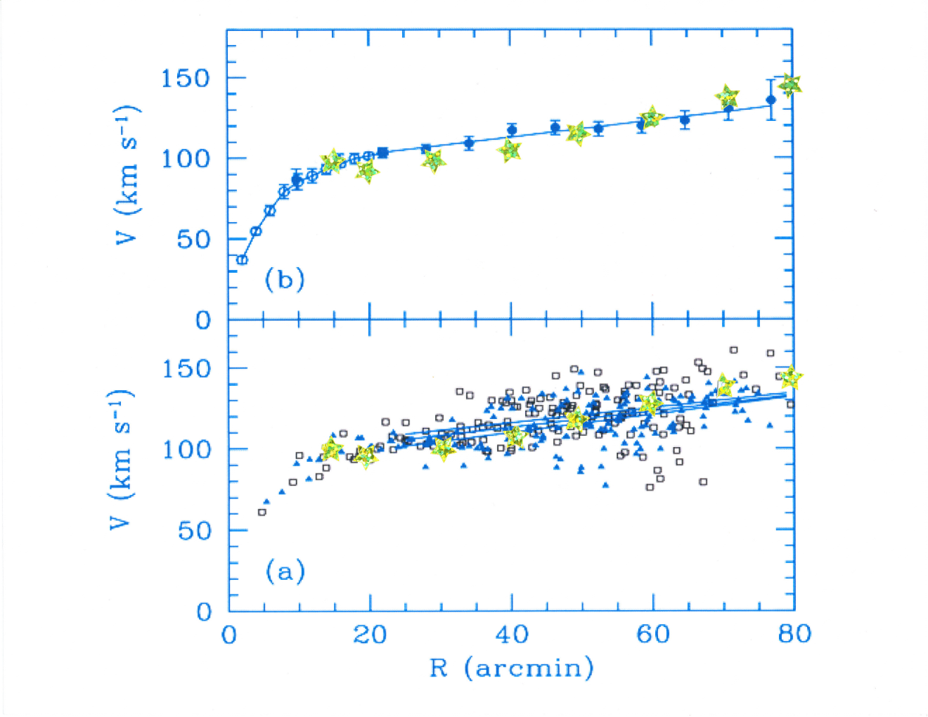
III.2.5 The Model Parameters Seem Acceptable.
In addition to the requirement that the model predicts observed rotation curves, one requires that the model parameters are reasonable. For the Milky Way, arbitrarily assuming kpc, one finds the ‘errors’ reflecting uncertainty in the choice of . Alternatively, using2121 21 The mean peculiar speed of DM objects in originating regions is designated by . In paper I it is suggested that the mean intrinsic rotational speed of a DM object is in equilibrium with its peculiar translational velocities. This numerical estimate assumes the DM objects have baryonic masses. and with Mróz et al 2019, one estimates ; the uncertainty reflecting the uncertainties in and . The probable range for the DM pressure is at to at .
For the large spirals, the extent of the observed haloes sets a lower limit to the value of . Using kpc, this range for needed looks reasonable. For both types (a),(b) of halos it is reasonable to adopt where is the effective density of DM in intergalactic space. These should be compared to other appropriate densities (See Bahcall 2000; Scott et al 2000.)The limiting cosmological critical density is . The mean densities of luminous matter in clusters of galaxies are ; this is on the order of our estimate for .
In the MW inner halo the DM pressure is corresponding to which is slightly smaller than the OM mean density of the MW galaxy distributed inside a sphere of kpc radius, . The local mean density of OM is estimated to be Mróz et al 2019.
For the representative small galaxy M33, we may estimate at kpc from . Because of the observed linearity of the rotation curve the value of is reasonably determined even though the value of is uncertain. One finds . The agreement of this value of with the value found for the large Milky Way galaxy suggests one ‘infall’ mechanism is sufficient to explain both types of rotation curves.
III.2.6 Improvement Of The Modelling Procedure.
To significantly improve these models one needs observations to estimate the amounts of ordinary matter entrapped within the DM haloes and flowing through the inner edge of the DM halo. Also, the mass of the OM disc population in the outer regions, is needed. It is possible that outer OM disk populations may cause ‘wiggles’ in the rotation curve. With a combined OM and DM model one could determine the density contribution of eq.(8).
This is important because the only model parameter not yet well determined is . Trials in fitting indicate is small, so to lowest approximation we used . To determine it from the rotation curves requires assumptions about the outer OM galactic disk density and the subsequent modification of . We do not have a theoretical estimate of this parameter. [See the discussion of eq.(8).]
III.3 Observational Challenges.
A main observational challenge is to determine the interface between the outer halo and the intergalactic medium and the value of . Observations of DM lensing Mandelbaum et al 2006 in earlier epochs are modeled with kpc. In the case of the MW galaxy,, which exhibits a flat rotation curve at , one has limits set by disturbances at kpc by the dwarf galaxies LMC & SMC, and at kpc by M31; evidently the assumption of a spherical gravitation potential would would be crude and useful only in selected directions. A study of MW ‘halo objects’ suggests the halo changes character at kpc and might extend to kpc [Battagia et al 2005]. Also very low surface brightness observations of emissions from ordinary matter trapped in the extended DM regions around galaxies would be rewarding in possibly mapping out motions in the halo.
It should be remarkably easy to use this procedure to represent the observed halo radial velocity curves of many galaxies. The derived model parameters may be used as a first probe of the variations in the intergalactic DM medium. There really is an interesting unexplored observational field here. There is no reason to assume that since the epoch of decoupling from ordinary matter, most of the DM (- of the total matter -) should remain anywhere near homogenously distributed in the Universe.
Not all galaxies enveloped in a DM intergalactic medium need have haloes such as those calculated. Our model requires that the peculiar velocities of a significant portion of the local DM be low. The components of DM carries intrinsic angular momentum which, combined with orbital angular momentum, forms a centrifugal barrier to prevent close approach to the center of attraction. (See Paper I.) The DM halo’s inner edge effectively starts at . A low mass galaxy may have its DM halo starting well beyond its visible structure. A high mass galaxy may have its halo structure begin inside its visible structure. The Milky Way probably is such a galaxy. So far, observations of other large spirals suggest values kpc. Any OM entrained with the DM at large distances, having only orbital angular momentum will fall through the DM barrier at . However one guesses it should be a minor halo component; one expects OM to constitute Tegmark et al 2004; Longair 2005 of the halo density at large .
III.3.1 Other Considerations.
We also note that DM with high angular momentum may provide the external pressure boundary condition needed to construct classic Bonner-Ebert models of protogalaxies. Ebert 1955; Bonnor 1956 Because of past galaxy-galaxy collisions, it would be impossible to rule out the presence of DM inside galactic disks. DM entrapped within galaxies by galaxy-galaxy collisions may thermalize and loose almost all its orbital angular momentum, thereby providing a confining pressure to aid form very massive star models.
DM with larger peculiar velocities than those assumed () could form haloes with similar structures but at much larger distances; this may provide models of galaxy lenses. We have not allowed for the presence of OM in the haloes. The presence of the Sunaev-Zeldovich effect, indicating the presence of OM , precludes direct application of these models to the haloes of galaxy clusters.
IV Summary.
A model of the dark matter (DM) surrounding galaxies has been developed which represents the observed rotation curves and can explain the absence of DM in small potential wells such as the solar neighborhood. The model is based on conservation of angular momentum in the flow of DM around a galaxy. In it (see Paper I) the DM is treated as a new state of matter in which matter while traveling along time-like paths also carries considerable transverse momentum. This transverse momentum results in intrinsic angular momentum terms. These, coupled to the usual orbital angular momentum, form centrifugal barriers, preventing DM objects from passing close to centers of gravitational attraction. In addition, the DM objects can transport an internal form of momentum. For aggregates of moving DM objects, the local sum of the internally transported momentum fluxes appears as a new form of ‘pressure’, not a thermodynamic pressure. For DM this term is large and must be included in specifying the energy-momentum tensor, the local source of the gravitational field and in calculating rotational velocities in the outer parts of galaxies. The halo cannot be primarily OM: (1) it is not seen; (2) there is no reason why OM halo material would be diminished in the region .
IV.1 Halo Structure
Two alternate forms of the energy-momentum tensor representing DM are derived in this paper. One features a large positive momentum flux appearing as a dominant pressure-like term. Using this the structure equations for the halo are developed and examined; these show that the pressure increases considerably as one approaches the central attractor but suffers an abruptly termination because of the centrifugal barrier. The DM matter forms an annulus around the central galaxy, a ‘halo’, and does not enter the central region.
In this halo region, the circular velocity is given by one of Einstein’s equations eq.(45). Here represents (mainly) the central OM galaxy’s gravitational potential and is small and slowly varying. In the outer halo regions , so constant. The variation of is determined by consideration of particle flux and angular momentum conservation.
A model for the Milky Way galaxy uses an inner edge of the halo at and an outer edge at ; the pressure there is , with the intergalactic DM pressure being perhaps a factor of 10 lower. The local intergalactic DM contributing to the MW halo seems to have low peculiar velocities . A model fitting the rotation curve of the small spiral M33 is constructed using only the inner structure of the halo; in it the centrifugal barrier is important.
Aggregates of such DM objects could comprise the main component of the intergalactic medium. Because of the gravitational attraction of an (ordinary matter) galaxy, the intergalactic DM medium locally compresses to form a galactic halo around a galaxy. One expects, because of variations in the local peculiar velocities of the DM objects, that the size of the halos would vary. Models of galactic haloes can be calibrated from observations with sufficient accuracy to provide a tool for investigating variations in density, pressure and the peculiar velocities of the intergalactic DM medium.
IV.2 Cosmology
The other form of for DM found can be made to resemble the conventional form of used in cosmology to represent ordinary matter (OM), providing a cosmological ‘constant’ term , slightly varying, is also introduced. This raises the possibility that at least some part of the ‘dark energy’ is not a separate entity but due to the representation of DM used.
If the alternate representation is adopted for cosmology, then is not constant and the Standard Cosmological Model would need some re-discussion. We do not claim this is the only reason for the term’s presence in Einstein’s equation, but this simple DM proposal provides a rationale for its presence. It is needed in modern cosmology to get the observed baryon acoustic oscillation spectrum and was based on the assumption that the DM was simply like an undetected form of ordinary matter with an ordinary fluid featuring a conventional relation. However, this spectrum represents only the epochs when the Universe was becoming transparent , when the optical depth is less than and does not justify the assumption that was constant at earlier epochs.
It is possible that varies on cosmological time scales. The observed cosmological parameters Longair 2005 would then represent an averaged ; it would very likely represent the value of when particle formation was frozen, i.e. when the temperature was Mev.
[(An earlier version of some of these ideas is available on-line Helfer 2017.]
V Appendices.
VI Appendix A: Astronomy.
VI.1 Inferred Properties Of Dark Matter.
There exist many large spiral galaxies (including the Milky Way) with ‘dark matter’ haloes. The observational characteristic of these spiral galaxy halos are galaxy rotation curves, consisting of: (1) a central spherical contribution followed by a (roughly) linear part : for kpc; (2) a (fairly) ‘smooth’ transition zone kpc; and (3) a roughly “flat” part for kpc. This outer limit is hard to estimate and in a few cases may be kpc. A value characterizes large spirals. Rubin 1980; Rubin 1983; Fich & Tremaine 1991; de Zeeuw & Franz 1991; Kulessa & Lynden-Bell 1992; Sofue & Rubin 2001. For the Milky Way see Mróz et al 2019.Read et al 2014.These rotation velocities2222 22 These are defined by the observed line-of-sight motions of extreme Population I objects such as very luminous HII regions or HI gas and molecular clouds, known to depart by less than from circular orbital velocities in galactic disks outside the very central region. The absence of these objects in the outer parts of galaxies limits our present knowledge of the rotation curves at large . are normally interpreted as circular velocities, setting where when and regarding as a true mass distribution. No galactic mass distribution compatible with the observed stellar distributions predicts this behavior in the outer zone Mihalas & Binney 1981. An unseen (‘dark’) matter component is usually hypothesized, probably amounting to several times the mass contribution inferred for the stellar and interstellar matter contribution. Because the halos are strongly concentrated to the center, the halo DM must be moving at non-relativistic velocities; this is also true for DM in clusters of galaxies: (in clusters) are conservative upper limits.
There is also a class of smaller spiral galaxies showing smaller halos whose outer rotation curves have an approximately constant positive slope. The small galaxy M33 studied in this paper -see Fig.2- may be considered a prototype.
Presently, there is no direct evidence that this ‘dark’ matter (DM) interacts with ordinary matter (OM) through electromagnetic interactions or collisions. However, in the standard cosmological model both types of matter remained coupled to radiation until eV. To be coupled the DM must have an interaction cross-section with . Allowing for the model’s uncertainties we note that for DM to remain coupled for energies down to eV (or KeV) one must have an interaction cross-section , if DM is represented by particles of baryonic mass. [If they have less than an electron’s mass, one has the additional problem of explaining their low velocities in galactic halos.] Also, such particles would be entrapped within a typical star like the sun if .
VII Appendix B: Supplementary Physical Arguments.
VII.1 The Vanishing Of The ‘Line’ Divergence
The technical point here is that we are are considering functions defined only along a line so we cannot directly use the Gauss divergence theorem with no sources or sinks present. However is a scalar, independent of a coordinate system choice. At any point, choose a geodesic coordinate system and rotate the coordinate axes so that is the coordinate along one of the axes. Then has only component, , and because is a geodesic’s tangent vector. For DM when we consider confluences of streams such as in a small region, we shall also assume to prevent local creation or destruction of streams; rigorously, in the presence of spin one only has established in the guiding center approximation.
VII.2 For Ordinary Matter.
We start with a method for constructing for ordinary matter (OM) when mass motions are significant and their associated momentum flux exceeds any assignable pressure term. An example is the rotating stellar disk in a spiral galaxy. It may be useful for numerical solutions to Einstein’s equations
The only formal requirements in GR on the fluid energy-momentum tensor are that it is symmetric and divergence-free ; consequently, a term , where is constant, can always be added to .
For each OM object with constant mass following the time-like path we define an energy momentum tensor by using the geodesic equation and requiring mass conservation. Set
| (17) |
along the path and determine the variation of by requiring
| (18) |
| (19) |
then and can be used as a fluid’s source term for determining the curvature tensor. So, for satisfactorily representing even one typical object as a source, one must introduce a ‘density’ distribution function. Then the distributed object may be thought of as equivalent to a localized stream with a finite cross-section and mass density .
One may show (see Appendix A) that if the objects are neither created nor destroyed in the region under study.2323 23 This divergence-free condition is equivalent to choosing the radiation gauge in EM theory. Henceforth we drop the accent, writing for when speaking of a ‘typical’ object. Then eq.(18) has three useful forms depending upon the functional form of available: (1) steady state one-dimensional pipe flow2424 24 i.e. For an aggregate of close-by objects all moving similarly, the argument of Appendix A1 holds and we can regard them collectively as a narrow confined stream of objects.:
| (20) |
(2) given the fluid form , the equation of mass continuity results,
| (21) |
where ; and (3), given the kinetic form , Liouville’s equation results,
| (22) |
which plays an important role in interpreting some stellar kinematics. Chandrasekhar 1942; Battagia et al 2005 Each of these equations hold only on a time-like path .
Eqs.(21,22) use an additional constraint, , for individual particles and for simple2525 25 We may need to allow for the exchange of energy and momentum among different components of the source terms. particle ensembles. It is needed when the total number of particles is conserved. For a fluid this concept has no meaning, so it must be imposed on fluid representations to enforce the particulate nature of matter.
[Depending upon the interval of space-time being studied, this condition can be somewhat relaxed if the total source term is broken down into a sum of constituent fluids. For example, consider radioactive decay of a nucleus . The number densities are modified, also their associated momenta are changed and 4-momentum is transferred to the radiation field tensor.. The fluid , representing each species, is changed, but their sum in the source term in GR is not. So, e.g. . But because the source term is inclusive we can use the ideal fluid form and ignore interactions such as particle destruction. Similarly for considering star densities and the formation of black holes and proto-stars. ]
Now, suppose we have a finite number of streams in a small region . Conventionally we treat as an energy-momentum reservoir and effectively define local fields , and extending throughout as averaged values of the included streams. [The averaging is detailed in text.] Then where only , expressing contributions from the variances of the velocity distributions, need require a thermodynamic equation-of-state to evaluate; its contribution is usually small for non-relativistic OM.
We emphasize that the spacial components of represent the streams’ average momentum flux Landau & Lifshitz 1959, and not really thermodynamic ‘pressure’ terms. The assumption of isotropy in cosmology allows confusion between the components of and of ; but in modeling individual galaxies it is the streaming motions of various galactic populations contributing to that are the source of the spacial terms in the stress tensor.
VII.3 The Halo Structure.
VII.3.1 Representation Of The Averaged In The DM Halo Model.
We use only DM with , so that the components of the basic energy momentum tensor are given by eq. (7), with the signs reversed to represent the source function. From eq.(8) we must add a contribution from the other source term ; for cold DM only the (positive) density term contributes. So, for the sum of the two contributions to the halo density we write , where is expected to be small.
First we derive eqs.(6, 7), slightly generalizing the notation to allow inclusion of anisotropic distributions of DM. In the halo annular region (e.g. in the spherically symmetric case) specify the halo by the change of from its value in the background model (at e.g. ). The halo material responds to the gravitational attraction of the central attractor, and the DM with sufficiently small angular momentum is compressed as it falls in. In type (b) halos DM falls inward from a stagnation zone on time-like trajectories at nearly parabolic2626 26 In the integral of energy conservation along a typical guiding center path, eq.(20) of Paper I, .speeds as judged by an observer at ; i.e. . In general we consider low-temperature halos in which at , the same is true and most of the DM objects have small peculiar velocities at distance and are isotropic.
We write for the change in a typical spacial diagonal component of at the halo point ,
| (23) |
Here is an average mass density, is the number of DM objects in a unit volume and represents a local value of one spacial component of . We consider only the major velocity contributors to these averages. For the isotropic case represents the square of the ‘speed’2727 27 Alternatively, this corresponds to transported locally along the mean ‘guiding center ’paths discussed in Paper I, and refers to that component of not involved in the internal ‘spin’ motion. of eq.(7). Here, and , so that is small for and one may write [A similar expression holds for in terms of the average value of .] Again, need not specify all the local DM, but just a particular subset.
Using the steady state one dimensional pipe flow, (see Sec. II) one has where is the speed along the fluid’s streamline . By eq(1) of Paper I, is very large compared to , and we may take it not very much affected by the gravitational field in the halo and we can set . Hence for halo DM
| (24) |
The density term, , can be expressed in terms of and the potential in eqs.(27, 28).
For non-spherically symmetric geometries, the rule to follow is that the vector component is transported along a particle’s world-line with the velocity . So, if in a local spacial Cartesian coordinate system, one has for the ensemble’s mass motion tensor only the diagonal elements , one should use
VII.3.2 Momentum Flux.
The pressure terms in eq. (7) represent a type of momentum flux. Statistical treatment of large numbers of streams of DM carrying momentum flux can be modeled after the standard treatment of radiative flux to introduce a momentum density. (See e.g. Chandrasekhar 1950; Rybicki & Lightman 1979.) Normally one writes for the energy (or momentum) crossing a surface element in a solid angle oriented at an angle to the normal of in a time interval ,
| (25) |
defining , the local specific intensity; it may be labeled by other parameters, such as the energy. Here is a velocity along the axis of the solid angle. The standard procedure is to focus on the development of , rather than , since it represents a ‘density’. One has e.g. , the energy density in isotropic radiation flows. For a steady-state when is independent of , the total transfer of flux crossing in one direction in unit time is . For us, dealing with momentum flux, of eqs. (23, 24), the local density of streams. For this momentum flux, , using . So to determine we focus on determining the flux of DM streams in a halo. For isotropic flows through concentric spherical annuli in free space one requires for flux conservation:
| (26) |
For the mass carried by the incoming streams one takes ; since conservation of mass gives constant along a stream-line, one has,
| (27) |
here is that component of perpendicular to the ‘spin’ plane, . (See eq. (20) of Part I.) In the outer part of the halo . In the inner part, one has determined by the gravitational potential (see Appendix C):
| (28) |
VII.3.3 Angular Momentum Conservation.
Now examine momentum conservation for a particular aggregate, with number density , of incoming DM objects which at large have specified low angular momenta; , considered as a function of , is subject to the constraint that each object in the aggregate must conserve its associated angular momentum in a spherical potential; the gas is collisionless.
Consider flow through a portions of a sphere; the normals of the area elements are the radius vectors. For convenience suppose at some large , in a volume element all the streams of objects considered have the same stream density and the same (small) average speed (where ).
For each stream of objects the orbital angular velocity is a constant and is determined just by the value of ( the angle between the 3-vectors and ). The total number of inflowing streams at a shell of radius is then , where is a distribution function for the ingoing streams. For large we adopt a distribution , corresponding to velocities being isotropic2828 28 The specification of is part of the specification of the angular velocity distribution; in principal it could be a function of . In near equilibrium the symmetries of the velocity distribution reflect the symmetries of the effective gravitational potential; see Chandrasekhar 1942 . so ; the collection of all these streams carries orbital angular momenta up to .
Let us follow such an aggregate moving in towards the center, assuming for convenience that is small enough that each stream follows a nearly parabolic orbit, i.e. , where is close to the galaxy’s maximum rotation speed. For any large , a similar argument gives for the inflowing streams. There is a region of ‘free-fall’ in which the streams are not appreciably deflected; in it so eqn. (26) is satisfied.
VII.3.4 The Inner Halo
Inside this region streams with large orbital angular velocity will be deflected. We calculate the loss to the inflow. In the background space suppose we regard each sphere represented by a (fictitious) collection of ‘bound’ DM circular orbits, each with an associated orbital angular velocity given by . For a falling stream to pass through a sphere of radius it must have its distance of closest approach to the center be less than .
For example, let with a constant, representing the (ordinary matter) inner part of a galaxy for . For a stream of DM particles following a parabolic orbit () one requires where represents the intrinsic angular momentum associated with the DM object (See Paper 1.) One has where . [ Bound circular orbits cannot be defined for DM for ] With parabolic infall velocities, DM objects have their turning point at .
Consider a particular sphere Only those streams with low reach ; they have the same (invariant) values of as they had when they were at . We calculate the fraction of inflowing streams at that can reach this particular ; one has , using as the variable of integration instead of :
| (29) |
This loss must be compensated for by an decrease in since the total number of streams with assigned which can travel from to is conserved. Consequently2929 29 Note we have not assumed that at our starting point, , is the maximum orbital angular velocity possible, . since , one has, for an inner zone
| (30) |
this definies . This holds3030 30 More general potentials can be used. We really assume that in the outer halo is an increasing function of , so that there is a limiting radius at which ‘free-fall’ ends and for which equation (30) holds. for all for which .
VII.3.5 The Boundary Between The Two Halo Parts.
The boundary between the two regions, , occurs at where
| (31) |
the RHS assumes is close to the inner halo edge where . This is true for only high mass galaxies and DM with low initial angular velocities, ; this is the case of most interest. Then the DM generally is in the free-fall zone where . But, for low-mass galaxies may be close to , severely limiting any ‘free-fall’ zone.
In this inner zone the change in the gravitational potential can be appreciable because of contributions from OM galactic disk populations and actually has a complicated behavior; by itself eq. (28) gives
| (32) |
VII.3.6 The Imput Parameter .
From the discussion in Section 3.2 in text one has for the Milky Way galavy, kpc. Using the approximation eq.(31) and kpc one estimates . Considering the uncertainty in , this is in good agreement with its estimate in text, based on the observed value of .
For the small galaxy M33, the estimate is more uncertain because less is observed and is not known. The text uses kpc and kpc for representing the rotation curve. For theoretical reasons, one expects to be ‘close’ to . If we use then eq.(31) inplies . If , then . Also, because of the natural width of the distribution of DM near its peak, , it is possible that a lower value for should have been inferred: kpc , resulting in increase in .
It is interesting, then, that both galaxies can be characterized by the same imput velocity, despite their differences in size and OM mass.
VII.3.7 Some Caveats.
The infall argument holds for ordinary matter as well as dark matter since it involves conservation of a flux, which may be a mass flux as well as a momentum flux. If some of the in-falling streams do not come from a real stagnant region and actually have appreciable mean stream velocities at large distances, the treatment would need modification, since the expression for holds only in the stream’s rest frame. In this paper, using our expression for , we are actually considering a restricted class of incoming matter and our estimates for densities, etc. at large distances refer only to them. Because of collisions, ordinary matter particles can exchange angular momentum and some part of the initial flow will always reach the central galaxy with very low angular momentum and fall in. But, as postulated, the DM particles always possess a non-zero total orbital angular momentum and cannot penetrate deeply into the central galaxy.
VII.3.8 Approximations For The Halo Pressure & Density.
For the region use as unit of length ( which shall turn out to be close to the maximum of the rotation curve for many cases of interest). Represent the intrinsic angular velocity by with the maximum orbital angular velocity of the incoming DM halo streams given by . For the form of adopted, . f One writes and estimates but in this section we allow for the possibility of a much larger value. The formal inner edge of the halo, defined in terms of the lowest bound ‘circular’ path is and the furthest inward DM parabolic orbits can go is ; we will use as representative in the approximations because we are interested only in infall with low angular momentum. In these units the boundaries of the inner zone are given by . We used in our models.
In the outer region one has, from eqs.(26,27):
| (33) |
ignoring the variation of the small quantity in the outer zone in calculating .
In the inner zone, using eqs. (27,30) we allow for the variation of in calculating the density. Using the notation and (so that in the inner zone ),
| (34) |
For the DM mass in the inner zone, using , one has
| (35) |
so that, using one has . Also, for the additional DM mass above the boundary, , in the outer zone, one finds
| (36) |
In the inner zone the pressure reaches a maximum at and then, going inwards falls rapidly to zero at . One finds the halo structure effectively starts at , i.e. for , may be taken as small. For , one may consider the pressure and density as approximately constant; they then fall as we go further out. For either type (a) or type (b) halos the size of the halo, using , is constrained by the angular momentum condition
| (37) |
where ; this imposes an important constraint on the choice of . With these expressions for the structure of the halo can be developed and the functions , used in defining the metric, can be calculated. See Appendix C.
VII.3.9 The ‘Shielding’ Distance
For type (a) halos, which may be quite extended, there is an additional feature because the model DM halo density may be negative if is small. In the limiting case one may define a ‘shielding’ distance, , such that
| (38) |
since for DM. This corresponds to and in Appendix C is used to define the edge of the halo . Since is For Using and , and for the outer zone . one finds using equation (45) for the observed asymptotic circular velocity, , that
| (39) |
where . For the MW galaxy . The significance of is that for the details of the potential representing the central attractor are no longer relevant and the metric coefficients are purely determined by the background intergalactic DM cloud. It is reasonable to consider for type (a) halos and this the proper definition of . Again, this value of is crude because the value of has been assumed low and we have neglected positive density contributions from OM trapped in the halo.
VIII Appendix C: Metric Parameters For A Galaxy’s DM Halo.
The DM halo is represented by the standard fluid energy momentum tensor (with ). When one has as a large pressure term and with. For outside this range,
VIII.1 Outside
The intergalactic medium is represented by the Robertson-Walker metric
| (40) |
where the structure equations are:
| (41) |
and the ‘energy’ conservation constraint
| (42) |
hold for . Here, we have added to the usual fluid source term. One can get a static model (with ) by choosing appropiately. For our case of the surrounding intergalactic cloud being purely DM, is the dominant term with being small and negative. For a quasi-static model take so that . Also so that one may take Then , having the dimensions of an inverse length squared, sets the scale of the curvature effects. For example, for one has l.y. Consequently, one may take for our halo models.
subsection The Form Of In The Halo.
In the Schwarzschild model (equation (6) of Paper I)) for the entire halo , we have where ; is the mass of the central attractor at and is given by eqns. (35, 36); For DM , The halo begins at with ; there one has . Eqs.(33, 34) give approximations for for the halo. Using these approximations for the mass variations one has
| (43) |
where . This matches There is a similar expression for for , resulting in e.g.
| (44) |
where has been used. One has and, for massive galaxies . [See eq. (31.] As noted in Appendix B, there is a limit to , provided by a shielding length , see eq.(39), if the (negative) halo density provides significant shielding. To join onto the exterior solution, theRobinson-Walker metric, at one choose the parameter appropriately.
VIII.2 The Form of In The Halo
The restriction requires . But this standard relation is not directly useful because: (1) have different dependences on ; (2) there are other neglected contributions, see eq.(8); and (3) has an additional contribution from the OM central galaxy. Also, the quantity may not be constant in the inner halo. In the outer parts of DM halos , the variation of is predictable and , mainly due to DM, can be directly determined from observations (since ) assuming strict circular motion. Generally other combinations of Einstein’s equations are more useful for determining approximations for the three quantities, . Because is small and its variations should have minor effects in the outer halo, we initially assume it constant.
For the Schwarzschild metric, we have . Again using , where is small in a halo model, one may rewrite this Einstein equation in a more useful form:
| (45) |
where is known -see the previous section- and for most of the halo is small. For our simplified version of for DM one has Both and are continuous at the joining points and . Using our approximations for the density, eqns.(33, 34) for , one has in the innermost interior halo zone. Next one has
| (46) |
For the outer zone, since , one has
| (47) |
for . Again , and [if there are no contributions from OM]. For large , one has constant.
VIII.2.1 The Outer Rim of the Halo.
In the outermost halo region, where is large and (see eq.(15)) one has
| (48) |
with
| (49) |
Here . In practice we use . Then, to satisfy the boundary condition at we suggest adding the small constant to throughout the entire region .3131 31 For the usual exterior Schwarzschild solution representing an isolated source , one chooses because the solution is supposed to hold as . Here we impose another boundary condition. We shall ignore it for although it may affect estimates of the shielding distance . Using eqs.(45, 15), one has
| (50) |
This shows both as . Since we only determine , see eq.(45), a constant may be added to it. We suggest requiring to satisfy the boundary condition . Then establishes the clock rate comparison inside and outside; this is to be expected because the halo is in a gravitational potential well with the halo model sitting on top of the background DM cloud model.
References
- Helfer (2019) Helfer, H. L. 2019, ApJ880, 73 . Paper I
- Yang & Liu (2018) Yang, Y. B. & Liu, Key-Fei, 2018 Phys. Rev. Lett.121, 12001
- Kolb & Turner (1990) Kolb,E. W. & Turner, M. S. 1990, The Early Universe (NY, Addison Wesley)
- Weinberg (1972) Weinberg, S. 1972, Gravitation and Cosmology( New York, Wiley)
- Chandrasekhar (1942) Chandrasekhar,S. 1942 Principles of Stellar Dynamics (U. of Chicago:Chicago)
- Battagia et al (2005) Battagia, G. et al 2005 MNRAS 364,433
- Landau & Lifshitz (1959) Landau,L. P. & Lifshitz, E. M. 1959, Fluid Mechanics (Pergamon: Oxford)
- Einstein (1950) Einstein,A. 1950, The Meaning Of Relativity, 5th ed. (Princeton:Princeton)
- Tegmark et al (2004) Tegmark, M. et al 2004 astro-ph/0310723v2
- Longair (2005) Longair, M. S. 2005, in IAU Symposium 201 “New Cosmological Data and The Values Of The Fundamental Parameters” , ed. by A. Lasenby and A. Wilkinson (Sheridan Books: Ann Arbor)
- Clemens (1985) Clemens, D. P. 1985 ApJ295, 442
- Mróz et al (2019) Mróz, P. , Udalski, A., Skowron, D.M., Skowron, J. Soszyński, I., Pietrukowicz, P. Szymański, M.K. ,Poleski, R., Kozlowski, S. and Ulaczyk, K.2019 ApJ870 L10
- Read et al (2014) Read, M. J.,Menten,K. M., Brunthaler,A. et al 2014ApJ783,130
- Trimble (2000) Trimble, V. 2000 in Allen’s Astrophysical Quantities, 4th ed.,edit. byA.N.Cox( Springer:NY)
- Mihalas & Binney (1981) Mihalas, D & Binney, J. 1981 Galactic Astronomy, 2nd ed. (W.H. Freeman:San Francisco)
- Bahcall et al (1983) Bahcall, J. N., Schmidt, M., & Soneira, R. M. 1983 ApJ265, 730
- Bahcall (1986) Bahcall,J. N. 1986 ARAA 24,577
- Gilmore (1984) Gilmore,G 1984 MNRAS 207, 223
- Bahcall (2000) Bahcall, N. A. 2000 Allen’s Astrophysical Quantities, 4th ed.,edit. A.N.Cox (Springer:NY)
- Scott et al (2000) Scott,D. et al 2000 in Allen’s Astrophysical Quantities, 4th ed.,edit. by A.N.Cox (Springer: NY)
- Ebert (1955) Ebert, R. 1955 Z. Astrop. 37,217
- Bonnor (1956) Bonnor, W. B. 1956 MNRAS 116,351
- Corbelli & Palucci (2000) Gorbelli, E. & Salucci, P. 2000 MNRAS 311, 411
- Kam, et al (2015) Kam, Z.S., Carignan, C., Chermin, L., Amnam, P., and Epinat, B. 2015 MNRAS 449, 4048
- Chandrasekhar (1950) Chandrasekhar, S. 1950 Radiative Transfer (Clarendon: Oxford)
- Rybicki & Lightman (1979) Rybicki G. B. & Lightman,A. P. 1979 Radiative Processes In Astrophysics (Wiley: New York)
- Mandelbaum et al (2006) Mandelbaum, R. et al 2006 MNRAS 368, 715
- Helfer (2017) Helfer, H. L. 2017 arXiv: gen-ph/1705.08746
- Rubin (1980) Rubin, V. C. 1980 ApJ238, 471
- Rubin (1983) Rubin,V. C. 1983 Science 220, 1339
- Fich & Tremaine (1991) Fich,M. & Tremaine, S. 1991 ARAA 29,409
- de Zeeuw & Franz (1991) de Zeeuw,T. & Franz, M. 1991 ARAA 29, 239
- Kulessa & Lynden-Bell (1992) Kulessa,A. S. & Lynden-Bell, D. 1992 MNRAS 255, 105
- Sofue & Rubin (2001) Sofue, A. & Rubin, V. C. 2001 ARAA 39, 137