Preferential concentration in the particle-induced convective instability
Abstract
Heavy particles in turbulent flows have been shown to accumulate in regions of high strain rate or low vorticity, a process otherwise known as preferential concentration. This can be observed in geophysical flows, and is inferred to occur in astrophysical environments, often resulting in rapid particle growth which is critical to physical processes such as rain or planet formation. Here we study the effects of preferential concentration in a two-way coupled system in the context of the particle-driven convective instability. To do so, we use Direct Numerical Simulations and adopt the two-fluid approximation. We focus on a particle size range for which the latter is valid, namely when the Stokes number is . For Stokes number above , we find that the maximum particle concentration enhancement over the mean scales with the rms fluid velocity , the particle stopping time , and the particle diffusivity , as . We show that this scaling can be understood from simple arguments of dominant balance. We also show that the typical particle concentration enhancement over the mean scales as . We finally find that the probability distribution function of the particle concentration enhancement over the mean has an exponential tail whose slope scales as . We apply our model to geophysical and astrophysical examples, and discuss its limitations.
1 Introduction
Preferential concentration is the tendency for heavy particles to accumulate in regions of high strain rate and low vorticity due to their inertia (Csanady 1963; Meek & Jones 1973; Maxey 1987). Investigations of the process date back to the 1980s and were performed using numerical experiments (Maxey & Corrsin 1986; Squires & Eaton 1991; Elghobashi & Truesdell 1992) and laboratory experiments (Fessler et al. 1994; Kulick et al. 1994). For comprehensive reviews of the topic, see for instance (Eaton & Fessler 1994; Crowe et al. 1996; Balachandar & Eaton 2010; Monchaux et al. 2012) and references therein.
Today, thanks to progress in high-performance computing, Direct Numerical Simulations (DNSs) are a particularly convenient tool for quantifying preferential concentration in particle-laden flows. A variety of techniques can be used, which can be loosely classified into two distinct approaches: the Lagrangian-Eulerian and Eulerian-Eulerian approaches (see Sections 2.1–2.2 for more detail). The Lagrangian-Eulerian (LE) approach is named for the fact that the particles are evolved individually by integrating their equations of motion, while the carrier fluid is evolved on an Eulerian mesh. Various degrees of sophistication exist, depending on whether the particles are modeled realistically using, for instance, immersed boundary techniques (Mittal & Iaccarino 2005), or in a simplified way, as point particles (Toschi & Bodenschatz 2009). In the latter case, particles can either be passively advected, or can react back on the fluid through drag. When particles are modeled exactly, the LE approach is capable of modeling particle-particle interactions, such as collisions. Otherwise, these interactions must be accounted for using simplified parameterizations instead. However, as the number of particles increases, the computational cost can be expensive. In the Eulerian-Eulerian (EE) approach by contrast, the particles are treated as a continuum field with its own momentum and mass conservation laws, which are evolved on an Eulerian mesh (Elghobashi 1994; Crowe et al. 1996; Morel 2015). Within the EE framework, various levels of approximation exist depending on the size of the particles, ranging from the so-called equilibrium Eulerian limit (Ferry & Balachandar 2002; Ferry et al. 2003) in which particle inertia is neglected, to the two fluid limit (Elghobashi & Abou-Arab 1983; Druzhinin & Elghobashi 1998) which is generally more valid for somewhat larger particles.
In regions of the fluid that experience strong local enhancement in the particle number density, increased collision rates can result in rapid particle growth (Cuzzi et al. 2001). As such, preferential concentration is thought to play an important role in controlling the size distribution function of particles suspended in turbulent fluids. Prior works have focused on certain aspects of preferential concentration such as the enhancement of the particle settling velocity (Aliseda et al. 2002; Maxey 1987; Wang & Maxey 1993; Mei 1994; Yang & Lei 1998; Bosse et al. 2006), the resulting geometry of the dense particle clusters (Cuzzi et al. 2001; Monchaux et al. 2010; Goto & Vassilicos 2006), and the underlying mechanisms responsible for inertial clustering of particles (Raju & Meiburg 1995; Obligado et al. 2014; Goto & Vassilicos 2008; Coleman & Vassilicos 2009). Preferential concentration likely plays a key role in the warm rain formation in clouds (Pinsky & Khain 2002; Falkovich et al. 2002; Riemer & Wexler 2005), protoplanetary disks (Klahr & Henning 1997; Chambers 2010; Cuzzi et al. 2008), estuaries (Eisma 1991; Voulgaris & Meyers 2004), and industrial applications such as sprays (Cao et al. 2000; Vié et al. 2015). In all of these examples, some of the key questions that remain to be answered are: (1) What is the maximum particle concentration enhancement that can be achieved anywhere in the fluid? (2) What is the typical probability distribution of the volume density of particles? And, (3) how do these quantities depend on the turbulent properties of the carrier flow?
While these questions have been primarily investigated in forced turbulent flows so far (Squires & Eaton 1991; Eaton & Fessler 1994; Bosse et al. 2006), they have not been studied extensively to our knowledge in the context of particle-induced buoyancy instabilities (e.g. convective or Rayleigh-Taylor). Such instabilities are particularly relevant in particle-laden turbidity currents, which play an important role in sediment transport (Meiburg & Kneller 2010). Although most research to date on particle-laden buoyancy-driven flows has been performed using in-situ or laboratory experiments (Hoyal et al. 1999; Maxworthy 1999; Parsons et al. 2001; Völtz et al. 2001), numerical experiments have only recently begun to be used in this context. The focus of these numerical studies can be categorized into two groups: (1) numerical tests, in which various formalisms (i.e. LE versus EE) are compared to one another (Chou et al. 2014; Chou et al. 2014; Chou & Shao 2016), and (2) application-driven studies, that investigate for instance how the rate of sedimentation is influenced by particle properties. It was shown that both particle size and particle volume fraction can control the resulting modes of instability (i.e. leaking, fingering, stable settling modes) from the initial RT instability configuration, affecting the subsequent evolution of the sedimentation process (Burns & Meiburg 2012; Burns & Meiburg 2015; Shao et al. 2017). However, numerical investigations whose primary focus is on preferential concentration in the particle-driven convective instability, specifically for two-way coupled systems have not been performed.
In this paper, we therefore study preferential concentration in the two-way coupled two-fluid formalism using DNSs of particle-driven convective instabilities. Section 2 describes the two-fluid formalism. In Section 3, we introduce our model setup and its governing equations. In Section 4, we present the results of the DNSs and investigate how certain parameters influence preferential concentration and the underlying turbulence. In Section 5, we present a predictive model that captures maximum particle concentration enhancement as a function of time and space. In Section 6, we look at the probability distribution function (PDF) of the relative particle concentration. Section 7 summarizes our results and discusses them in the context of geophysical and astrophysical applications of particle-laden flows.
2 Two-fluid formalism
The two-fluid formalism for particle-laden flows can be derived starting from the Lagrangian-Eulerian formalism by locally averaging the particle properties to obtain the continuum density and momentum conservation equations. This essentially follows the derivation of Ishii and Mishima (Ishii & Mishima 1984) (see also (Ishii & Hibiki 2010; Delhaye & Achard 1976)). The formalism has been widely used within the astrophysics community for studying protoplanetary disks (Youdin & Goodman 2005; Nakagawa et al. 1986), as well as in studies related to sediment transport in rivers and oceans (Hsu et al. 2004; Bakhtyar et al. 2009; Revil-Baudard & Chauchat 2013), for instance.
For simplicity in this work, we focus on particulate flows in which the particle solid density is much larger than the mean density of the fluid , such as droplets or aerosols in the atmosphere or dust in accretion disks. We also assume that the particles are spherical, monodisperse, and dilute (ensuring that particle-particle collisions do not dominate the particle evolution equations).
2.1 Lagrangian formalism
Under the above assumptions, we can model the motion of a single particle interacting with the fluid through Stokes drag by solving the coupled ordinary differential equations
| (1) |
where is the position of the particle, is its velocity, is the fluid velocity at , is gravity, and is the particle stopping time. In (1), we have assumed that the reduced mass (which would normally multiply ) is approximately 1 since . We have also neglected other effects such as the Basset history and Saffman lift terms for the same reason (Maxey & Riley 1983).
To model a collection of monodisperse particles using the LE approach, (1) is integrated separately for each particle in the fluid:
| (2) |
where and are the position and velocity of the th particle, respectively. The back reaction of the particles on the fluid is accounted for by adding a mean local drag force in the Navier-Stokes equation (shown here in the limit of the Boussinesq approximation (Boussinesq 1903; Spiegel & Veronis 1960)):
| (3) |
where is the density deviation away from the mean fluid density , is the pressure, is the kinematic velocity of the fluid, and is explicitly defined as
| (4) |
where is the Heaviside function, is the particle mass, and is the volume of a sphere of radius . The averaging radius is typically chosen to be one grid cell in numerical computations. Equations (2)- (4), together with the fluid incompressibility condition , form the Lagrangian-Eulerian equations. These can now be statistically averaged using methods motivated from kinetic theory to derive the two-fluid formalism.
2.2 Two-fluid formalism
We first define the local mass density of particles and corresponding velocity , averaged in a small volume centered around the position as
| (5) |
Applying this average to the particle evolution equations in (2) (as done in (Ishii & Mishima 1984), for instance), we approximately get
| (6) |
where is the derivative following the mean particle velocity. The evolution equation for the particle density can be obtained by mass conservation to be
| (7) |
In both equations, dots on the right hand side result from three possible sources: (1) dispersion in both mass and momentum conservation equations due to the fact that ; (2) unaccounted for interactions of the particles with the fluid, which include Brownian motions for very small particles, and self-interaction of the particle with its own wake if the latter is not perfectly modeled by the Stokes solution; and (3) long-range interactions of particles with one another due to each other’s wakes. Aside from Brownian motions, these terms are generally very difficult to model, leading to strong anisotropic dispersion, and likely to depend nonlinearly on the mean particle density and velocity.
In what follows, we will model these terms for simplicity as in the momentum equation and in the density equation, so
| (8) | ||||
| (9) |
These terms are included to stabilize the numerical scheme in the DNSs, although they are also physically motivated in the limit where Brownian motion is the dominant source of dispersion. Note that we anticipate the two-fluid approach to break down when the Stokes number (the ratio of the stopping time to the eddy turnover time) approaches unity, in which case the particles become uncorrelated with the fluid and therefore also with one another (Shotorban & Balachandar 2006). When this happens, the mean particle velocity is no longer a good approximation for each individual particle velocity, and the averaging procedure becomes meaningless.
To couple the particle and fluid evolution equations, note that the drag term in the continuum limit in (3) becomes
| (10) |
so the two-way coupled equations are
| (11) | ||||
| (12) | ||||
| (13) | ||||
| (14) |
For smaller particles that are well-coupled to the fluid, the two-fluid formalism recovers the equilibrium Eulerian formalism in which particle inertia is negligible. We can demonstrate this by taking the formal limit to obtain:
| (15) | ||||
| (16) | ||||
| (17) | ||||
| (18) |
where the settling velocity is related to the stopping time and gravity via . The particle velocity is now determined by the carrier fluid velocity and the particle settling velocity. Compared to the two-fluid formalism, we see that ; thus, the particle concentration is solely advected by the carrier flow. As a result, preferential concentration cannot be captured by the equilibrium Eulerian approach (Maxey & Riley 1983).
3 The Model
3.1 Model set-up
We investigate particle-driven convective instabilities in a dilute suspension using the two-fluid equations. For convenience, we rescale the particle density with the mean density of the fluid, which defines . Having assumed that , it is still possible to have of order unity even though the volume fraction of particles is assumed to be very small. We assume that the carrier fluid has a constant stable background temperature gradient in the vertical direction, with the background temperature profile given by . This assumption was originally motivated by applications in which the carrier fluid is typically stratified, such as in warm clouds or rivers, but does not directly impact the results presented in this paper. Perturbations in the density of the carrier fluid are caused by temperature fluctuations around that background profile, and are related via , where .
In the limit of the Boussinesq approximation, the governing dimensional equations are then
| (19) | ||||
| (20) | ||||
| (21) | ||||
| (22) | ||||
| (23) |
where and .
Using this system of equations, we shall study the evolution of the relative particle density . To do so in the context of the convective instability, we start with initial conditions that take the form of a Gaussian profile of amplitude and width :
| (24) |
to which low amplitude random fluctuations are added, and where is the height of the computational domain. The initial particle velocity is set to be the particle settling velocity , while the carrier fluid is initialized with zero velocity.
3.2 Non-dimensionalization
We define the units of length , relative particle concentration , and temperature as
| (25) |
We can define a characteristic velocity for the fluid by identifying its kinetic energy with an estimate of the potential energy of the unstable particle density distribution:
| (26) |
The characteristic distance and velocity can finally be used to construct a typical convective eddy turnover time
| (27) |
Thus, the non-dimensional equations are:
| (28) | ||||
| (29) | ||||
| (30) | ||||
| (31) | ||||
| (32) |
where all the variables are from here on implicitly non-dimensional, and where the dimensionless parameters are defined as:
Four of these parameters describe diffusive effects: a Reynolds number for the fluid , a Reynolds number for the particles , the particle Pclet number , and the temperature Pclet number . In the fluid momentum equation, is the density ratio, defined by analogy with double-diffusive systems to be the ratio of the density gradient due to temperature stratification to the density gradient due to particle stratification, here estimated as . In addition, is the non-dimensional stopping time, and is the non-dimensional settling velocity of the particles. Note that our non-dimensionalization defines as the ratio of the particle stopping time to the estimated turnover time of the layer-scale eddies. Thus, by construction, is an estimate of the Stokes number of the convectively turbulent flow.
We define the non-dimensional total density (i.e. consisting of the fluid and the particles) in the system as
| (33) |
so the non-dimensional total background density gradient is
| (34) |
The total density gradient controls the development of the convective instability and, as shown above, is the sum of the density gradient due to the temperature stratification and the density gradient due to the particle stratification. At time , the non-dimensional initial condition for the particle concentration is
| (35) |
The particle density gradient is most unstable at the lower inflection point of the Gaussian (), where it is equal to
| (36) |
Thus, the total density gradient at the lower inflection point at is
| (37) |
Using this information, we define a Rayleigh number as
| (38) |
where all the quantities on the right-hand side are dimensional. We can then express (38) in terms of the previously defined dimensionless parameters as
| (39) |
To ensure that overturning convection (rather than double-diffusive instabilities) takes place in all that follows, we set . We shall then vary by varying either or , ensuring in all cases that is sufficiently large for turbulent convection to take place. Finally, the Prandtl number will be fixed and equal to one for the flow to be fairly turbulent for all simulations. This choice fixes the relationship between and :
| (40) |
4 Numerical Simulations
Since our goal is to characterize preferential concentration of the particles by the fluid, which is an inherently nonlinear phenomenon, we must use DNSs. In order to do so, we use the triply periodic pseudospectral PADDI code (Stellmach et al. 2011; Traxler et al. 2011) which has been extensively used to study fingering as well as a number of astrophysical instabilities such as semi-convection and shear (Moll et al. 2016; Garaud & Kulenthirarajah 2016). A slightly modified version of the code was also used to study fingering convection in the equilibrium Eulerian regime (Reali et al. 2017). We have modified the PADDI code further by adding a particle field which evolves according to the two fluid equations (19) - (23), and refer to the new version of this code as PADDI-2F. Salient properties of PADDI, as well as the modifications made to include the two-fluid formalism, are briefly described in Appendix A.
In what follows, we present 2D and 3D simulations with specifications listed in Table 1. The size of the computational domain is selected based on the following considerations: (1) since the code is triply-periodic, the domain height must be sufficiently large to avoid unphysical interactions between the particles that leave the domain at the bottom and re-enter it at the top. With that in mind, we present simulations with height ranging from to . (2) The domain width must be chosen to be large enough to ensure that there are enough convective eddies in the horizontal direction to have meaningful statistics. In all the simulations presented below , and for 3D simulations, we further choose .
4.1 Two-fluid code validation against Eulerian simulations
To validate the PADDI-2F code, we begin by comparing a two-fluid simulation with low solving equations (28) – (32) with that of an equilibrium Eulerian simulation solving (15) – (18) (used in (Reali et al. 2017)). In both codes, we set , , and (corresponding to ); for the two-fluid simulation, we additionally set the particle stopping time to be , which should be sufficiently small to be in the limit where the equilibrium Eulerian formalism is valid. We first compare the two codes using 2D simulations (see Section 4.4 for a comparison of 2D vs. 3D simulations). We set the resolution of the 2D runs to be equivalent grid points in the and directions, respectively, and set the domain width and height as and .
In the snapshots presented in Figure 1, we see the evolution of the particle concentration and the horizontal component of the fluid velocity in the two-fluid simulation. Snapshots of the Eulerian simulation (not shown) taken at the same times look very similar to the two-fluid simulation (bearing in mind the chaotic nature of the system). The initially unstable total density stratification drives the growth of convective eddies, which become visible in the second snapshot (). The particle layer then rapidly spreads vertically under the effect of turbulent mixing in the third snapshot (), reducing the unstable particle gradient. Although there are horizontal inhomogeneities in the particle concentration, these remain small compared with the horizontal mean. In particular, never exceeds the initial maximum value of one, consistent with the expected properties of an advection-diffusion equation when . This shows qualitatively that for sufficiently small , the two-fluid simulation recovers behavior expected in the absence of particle inertia.

We now compare these simulations more quantitatively by examining the behavior of both the particle concentration and the fluid velocity. In order to do so, we define a number of diagnostic quantities (for convenience listed in Table 2). We first define the maximum particle concentration and maximum horizontal fluid velocity in the domain at any point in time as
| (41) |
We have selected to look at the behavior of the horizontal component of the velocity, rather than its vertical component or total amplitude, because it is not directly influenced by the particle settling motion.
In order to study the evolution of the bulk of the particle layer, we next define the horizontally averaged particle concentration profile , where the overbar denotes a horizontal average, as in for any quantity . The quantity can be compared to the corresponding analytical expression obtained when the particles evolve purely diffusively, namely when
| (42) |
The solution of (42) in an infinite domain with initial condition given by (35) is
| (43) |
As long as , this solution is also a good approximation to the diffusive solution in the periodic domain.
We also extract the maximum value of at time , which occurs at the height
| (44) |
In what follows, the asterisk will always indicate a quantity measured at the position . We can compare and to the maximum value of the diffusive solution, namely
| (45) |
Finally, we define the root mean square of the component of the fluid velocity at a particular height and time , expressed as
| (46) |
We can study turbulence in the bulk of the particle layer over time by extracting the corresponding value of at the position , defined by
| (47) |

Figure 2 shows a comparison of and for the particle concentration (Figure 2a) and and for the fluid velocity (Figure 2b) for both the two-fluid and equilibrium Eulerian simulations. Notably, we see that all the measured quantities are statistically consistent with one another in the two cases, verifying that the two-fluid formalism recovers the equilibrium Eulerian formalism for small . At early times () prior to the development of the convective instability, and follow the purely diffusive solution , shown as the black dotted line given by (45). Later, we see that and decrease rapidly (at times ), then more slowly again after . During that time and roughly decay at the same rate.

Looking at the eddy velocities, we see that the intermediate phase () corresponds to the peak of the mixing event. The corresponding reaches a maximum value of with the rms velocity reaching . The fact that and are both of order unity actually holds for all runs (see later), and proves that the non-dimensionalization selected is appropriate. By , the main mixing event is over and the turbulence (as measured both by or ) now gradually decays on a much longer timescale.
We can also look at how the particles and the fluid velocity evolve spatially over time. Figure 3 shows the profiles of and at three instants in time for both simulations, with the black dotted curve representing (43). Recall that the domain is periodic in both directions so the particle layer re-emerges at the top after leaving from the bottom. The dotted vertical line marks the position of the maximum of . We clearly see that the two-fluid and equilibrium Eulerian simulations behave in a quantitatively similar way. In both cases, the particle layer settles roughly at the expected rate set by the value of , but its vertical density profile becomes asymmetric and wider than in the purely diffusive case (black dotted line). The extended tail of below the bulk of the layer is associated with more rapidly-moving particle-rich plumes that can clearly be seen penetrating into the lower particle-free fluid in Figure 1. Focusing on the evolution of the profile, we see that at early times the turbulence develops in the bulk of the particle layer as expected. However, the fluid remains turbulent even after the particles have settled through a region, which explains why the size of the turbulent region is much larger than that of the particle layer at late times (e.g. ). This can be understood by noting that the time it takes for turbulent motions to decay viscously is much larger than the time it takes for the particles to settle across the bottom of the box.
This section has illustrated the interplay between the turbulence and the particle field for short stopping times. Both the qualitative and quantitative evidence confirm that the two-fluid model for very low and the equilibrium Eulerian model have similar dynamics, conclusively validating our two-fluid code.
4.2 Comparison between low and high simulations
We now look at the effect of larger stopping time on the evolution of the particle layer. We continue to work in 2D and choose with the same resolution (i.e. grid points) keeping the remaining parameters and domain size the same as in the simulation from Section 4.1 (i.e. , , ; and , ). Snapshots of the particle concentration field as well as the evolution of and with time are shown in Figure 4. We clearly see the emergence of regions of much higher particle concentration than at low , located in narrow, wisp-like structures (see for instance the snapshot at ) with reaching values of as high as 5. The fact that this is much larger than the initial maximum value of in the domain is a distinct signature of preferential concentration, since this only occurs when is non-zero. This also shows that regions of strongly enhanced particle concentration can develop even when the mean particle concentration in the bulk of the layer is decreasing. After the main mixing event (around ), drops again to values that are lower than one, though remains substantially higher than . This raises the interesting question of what determines the maximum possible value of the particle concentration field at any given time in the simulation (which will be further discussed in Section 5).

Turning our attention to the evolution of and , we see that for larger at the peak of the mixing event, and , whereas in the lower case the corresponding values were and . This suggests that does not have a major effect on the turbulence of the system (at least for the parameters explored).
We can measure the maximum particle concentration at a given height in the domain using
| (48) |
In addition, we can also measure the typical (rather than the maximum) enhancement over the mean as a function of height using
| (49) |
Figure 5 compares the maximum particle concentration with both the mean particle concentration and one standard deviation above the mean, , as a function of height, for two simulations with and . We see that for both cases, and have similar profiles. For the low case, typically remains below one. In addition, the profile of also follows that of , and lies about two standard deviations above it. As such, it is largest in the bulk of the particle layer. For high , is also largest in the bulk of the particle layer, with values peaking at at this particular instant in time. However, is now several standard deviations above , implying that the probability density distribution of the particle concentration has a longer tail (see Section 6 for more on this point).
Figure 6 more generally compares the maximum particle concentration obtained in several simulations with increasing particle stopping time . The simulations continue to be in 2D with grid points, and all other parameters remain unchanged (i.e. , , ). The black dotted line represents . As expected, we find that increases with as a result of preferential concentration. Furthermore, we see that remains above unity for longer times, signifying that dense particle regions persist in the simulations. On the other hand, we find that preferential concentration is negligible for , and is almost indistinguishable from that obtained in the equilibrium Eulerian limit.

4.3 Impact of and
We next look at the impact of the fluid Reynolds number and the particle Pclet number on the evolution of the particle concentration. We continue to focus on 2D simulations, choosing a relatively large stopping time to ensure that inertial effects are important. We use with the remaining parameters and domain size set as , , , and . The resolution selected for these simulations increases with both and , and is listed in Table 1. Figure 7 presents snapshots of the particle concentration at for simulations with and both varying between 1000 and 10,000. When we fix and increase , the particle concentration snapshots appear qualitatively similar, consisting of narrow structures comparable in size and density. The maximum particle concentration enhancement appears relatively unaffected by the fluid viscosity (at least, for this range of , and within the context of the two-fluid equations). In contrast, if we fix and increase , we see a striking difference in both the geometry of the wisps, as well as the maximum concentration achieved in the wisps. That is, as increases, these structures become more numerous and narrower, with a corresponding increase in the maximum particle concentration.

These qualitative trends are confirmed more quantitatively in Figure 8, which shows the maximum particle concentration as a function of time for each of these five simulations. We see that the evolution of is more or less independent of the Reynolds number but increases with Pclet number. This trend will be explained by the theory presented in Section 5.

In order to gain a more quantitative insight into the two-way coupling between the particles and the turbulence at all scales, we look at the power spectra of the particle concentration field and of the fluid velocity field. This time we restrict our analysis to an interval of time during the peak of the mixing event when the particle concentration is largest. We define the time-averaged horizontal power spectrum of a quantity as
| (50) |
where the is the discrete Fourier transform of and is the complex conjugate of . Figure 9a shows the horizontal power spectrum of the particle concentration field . When is fixed and increases, we observe a slight increase of power in the range , but the effect of is small. On the other hand, for fixed and large values of , there is substantially more power in the higher wavenumbers, consistent with the predominance of smaller scales seen in the snapshots.
In Figure 9b, we plot the power spectrum of the total fluid velocity field as function of . Unlike the particle concentration field, the spectrum here is affected by both and . That is, the amount of energy at small scales increases when either or increases. This can be explained by the fact that the strength of convection in our system is directly related to the Rayleigh number, which is proportional to the product of and (39). It is therefore not surprising to find that the energy spectrum depends on the product rather than and individually.

We also look at how the particle stopping time affects the horizontal power spectra of the particle concentration and velocity fields. Figure 10 shows these power spectra (taken, as before, during the peak of the mixing event), for five simulations at varying and otherwise fixed parameters (i.e. , , ; and , with resolution for simulations found in Table 1). In Figure 10a, we see more power at large as increases. We see this as further evidence that the particles increasingly concentrate in narrower wisps as increases. In Figure 10b, profiles of the total velocity power spectrum, i.e. , are strikingly similar to one another. Thus, does not appear to affect the turbulence in the system which is somewhat unexpected given the two-way coupling; instead, the velocity power spectrum is primarily dependent on , at least for the range of parameters explored here.

4.4 Comparison between 2D and 3D simulations
Owing to the high resolution needed for the two-fluid simulations, especially for higher , , and , 3D simulations are typically prohibitive. However, we have run several 3D simulations at moderate , , and in order to compare the 3D results with the 2D ones. In this manner, we can determine whether 2D results can at least qualitatively capture the properties of the particle layer evolution. For all 3D simulations, we set the non-dimensional length, width, and height as , , and , respectively. In this section, we focus on two simulations with and , respectively. The resolution of the low case is grid points, while the high case has a resolution of grid points.
Figure 11 shows that the values of achieved in the 2D simulation are consistently larger than the 3D simulation by 30-50% (for both low and high cases). This result is consistent with those of (van der Poel et al. 2013) for Rayleigh-Bénard convection (where the rms velocities in 2D are systematically larger than in 3D by a factor of about 2). As a result, turbulent mixing and preferential concentration are both more energetic in 2D than in 3D at otherwise similar parameters. For low where preferential concentration is not present, enhanced turbulent mixing results in being slightly smaller in 2D than in 3D. By contrast at high , is slightly larger in 2D than in 3D due to the enhanced preferential concentration. Generally speaking, however, the dimensionality of the model does not appear to affect preferential concentration by more than a constant factor of a few (see more on this below), suggesting that 2D simulations are appropriate, at least as far as extracting scaling laws is concerned.

5 Predicting maximum particle concentration
We now present a simple model to quantify the effects of preferential concentration in convective particle-driven instabilities. We begin with the particle concentration equation (30), substituting (where is the position vector):
| (51) |
By expanding the divergence term, we note that only the second term on the left-hand side contributes to preferential concentration (when ). We next assume that in the fully turbulent high flow, regions of particularly strong particle concentration enhancement are characterized by a dominant balance between the preferential concentration of the mean particle density and diffusion terms of the perturbations so that
| (52) |
We then express the particle velocity in terms of and u, using a standard asymptotic expansion in (Maxey 1987):
| (53) |
and thus,
| (54) |
Substituting (54) in (52) results in
| (55) |
Assuming that the length scales of the inertial concentration and diffusion terms are the same, we finally get
| (56) |
where the third part of this equation is expressed dimensionally. In this model, we therefore predict that strong particle concentration enhancements above the mean only depend on the magnitude of the fluid velocity u, the particle stopping time , and the assumed particle diffusion coefficient . The prediction (56) made for should hold in a large-scale sense (i.e. a scale greater than several eddy scales), and can help quantify the expected spatiotemporal evolution of as long as that of and is known.
In order to test our model, we have run a large number of 2D simulations (with a few 3D ones) at different values of , , and , listed in Table 1. Since the particle layer is not much wider than the size of an eddy, we investigate the validity of the model here only as a function of time, focusing on the behavior within the bulk of the particle layer (i.e. near ). To estimate the maximum particle concentration enhancement in the bulk of the particle layer, we let and find the maximum value of at each instant in time to obtain
| (57) |
To estimate the corresponding typical fluid velocity, we define the rms total fluid velocity found within the particle layer, defined as
| (58) |
where and for 2D simulations.
In Figure 12, we plot versus for one simulation (, , , and ). Note that each data point represents an instant in time for which the full velocity and particle fields are available. Points start from the lower left corner and move up to the right as increases with time during the development of the convective instability. During the most turbulent stage of the simulation when particle concentration enhancement occurs, the points are clustered on the upper right-hand side of the plot. The dashed line represents the scaling relationship, shown here for ease of comparison with later figures.

| (a) 2D Simulations | ||||
|---|---|---|---|---|
| 0.1 | 0.005 | 1000 | 1000 | |
| 0.1 | 0.005 | 10,000 | 1000 | |
| 0.1 | 0.005 | 100,000 | 1000 | |
| 0.1 | 0.01 | 1000 | 1000 | |
| 0.1 | 0.05 | 1000 | 1000 | |
| 0.1 | 0.1 | 1000 | 1000 | |
| 0.1 | 0.1 | 3000 | 1000 | |
| 0.1 | 0.1 | 10,000 | 1000 | |
| 0.1 | 0.1 | 1000 | 3000 | |
| 0.1 | 0.1 | 1000 | 10,000 | |
| 0.1 | 0.2 | 1000 | 1000 | |
| 0.1 | 0.3 | 1000 | 1000 | |
| 0.3 | 0.005 | 1000 | 1000 | |
| 0.3 | 0.01 | 1000 | 1000 | |
| 0.3 | 0.05 | 1000 | 1000 | |
| 0.3 | 0.1 | 1000 | 1000 | |
| 0.3 | 0.2 | 1000 | 1000 | |
| 0.3 | 0.3 | 1000 | 1000 | |
| (b) 3D Simulations | ||||
|---|---|---|---|---|
| 0.1 | 0.005 | 1000 | 1000 | |
| 0.1 | 0.1 | 1000 | 1000 | |
| 0.1 | 0.2 | 1000 | 1000 | |
Comparisons between and are next shown in Figure 13 for all available simulations that have , and . Here, the color of the points represents , the shape of the points represent , and the size of the points corresponds to the dimensionality (2D vs. 3D), see legend for detail. For a given simulation, each point corresponds to a particular instant in time selected after the onset of the convective instability, but before the bulk of the particle layer has traveled more than one domain height (to avoid it interacting with itself). The solid line shows the relationship , where the proportionality constant was selected to fit (approximately) the 2D data in the higher runs.
Focusing our attention first on the low 2D simulations (shown in red and orange), we see that they do not fit the model, regardless of the values of . This is as expected, since we have found that preferential concentration is negligible for (e.g. Figure 8), and so the dominant balance assumed in deriving the model in equation (56) does not apply. Turning to the remaining 2D simulations, we see the data fits the predicted model well albeit with a significant scatter that is expected given the method we are using to extract and . We also see that even for cases with larger , there appears to be a threshold (namely ) below which the model is not valid. Above that threshold, the scaling law proposed correctly predicts how evolves in a simulation as a function of time. Finally, we have run several 3D simulations represented by the larger filled circles, and see that they also fit the model. We therefore conclude that equation (56) provides a reliable method for estimating the maximum possible particle concentration enhancement over the mean in a turbulent fluid (within the two-fluid formalism).
Figure 14 explores the dependence of the model on and . As before, the low simulations (in red) do not fit the model while those at higher (all other colors) do. We also see that, as discussed in Section 4.3, is more or less independent of , but increases with .


6 Typical particle concentration and pdfs of the relative particle concentration field
Having constructed a simple analytical model for the maximum particle concentration enhancement allowable in the system, we may wonder whether this model might also provide insight into the typical concentration enhancement. To do so, we define the typical concentration enhancement within the particle layer as:
| (59) |
where was defined in (49). Results are shown in Figure 15, with the same black line as in Figure 13 also plotted to ease the comparison. Here, we see the data points do not fit this model, and seem to scale as instead (shown by the blue line). It is interesting to note that although we are capturing the typical enhancement, this model still depends on the same combination of parameters (i.e. the product of , and ) arising from the model discussed in Section 6. This strongly suggests that the typical particle concentration enhancement is related to the maximum particle concentration enhancement, though exactly how remains to be determined. We also see here that the low simulations (in red and orange) do not follow the same scaling law as the high cases, but instead, have almost constant.

More insight into the problem can be gained by looking at the probability distribution function (PDF) of the relative particle concentration:
| (60) |
We focus on values of within the bulk of the particle layer in the range , . Figure 16 shows PDFs of for the low and high cases presented in Section 4.4 at various times during the respective simulations. Prior to the onset of turbulence the PDF of is a function centered at since . The distribution then widens once the instability develops, and the maximum value achievable by is equal to the value discussed in Section 6.

For the low case, we see from Figure 16a that the PDF is more or less symmetric about at all times, and remains relatively narrow around this mean value (at least, compared with the high case described below). As the simulation proceeds, the width of the PDF first increases and then decreases with time, as a result of the concurrent increase and decrease of the turbulent fluid velocity (47) in the bulk of the layer during the convective mixing event. In contrast, for the high simulation shown by Figure 16b, the PDF widens considerably during the convective mixing event and becomes asymmetric. A long tail of rare events associated with preferential concentration appears. The shape of the tail appears to be exponential, consistent with what is commonly found in Eulerian-Lagrangian simulations of preferential concentration (e.g. (Shotorban & Balachandar 2006; Zaichik & Alipchenkov 2005)).
To explore the properties of this exponential tail, we present PDFs of taken during the peak of the mixing event for different simulations at fixed and for varying in Figure 17a. We observe that as increases, the slope of the exponential tail becomes shallower as the maximum value of achieved in the simulation increases. In Figure 17b, we present PDFs of for varying and at fixed , taken again at the maximum of the mixing event. We see that the tail widens with increasing but not with , which is consistent with our finding that does not directly influence the maximum particle concentration achievable (at these parameter values and in this model), but on the other hand does.

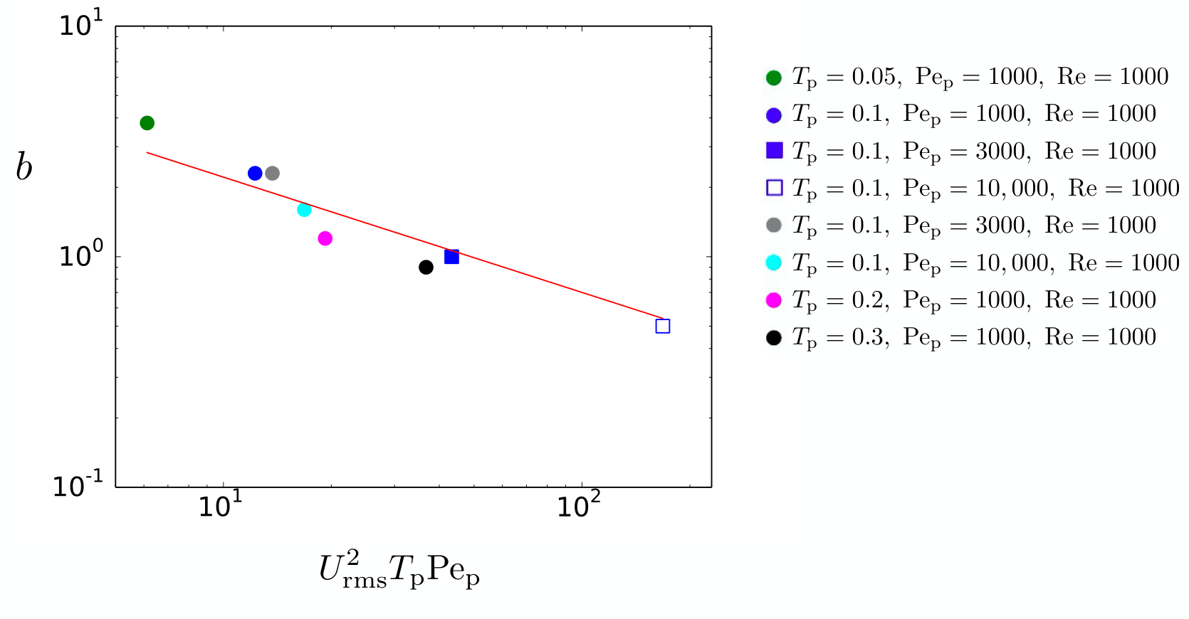
We have fitted an exponential function to the tail of the PDF for each of the cases described above. Figure 18 shows as a function of (where and are computed at the same times). We find that , which is the same scaling for . This is perhaps not a coincidence, since the rms of would be equal to if the distribution was exactly exponential with slope .
7 Summary, applications, and discussion
7.1 Summary
In this work, we studied preferential concentration in a two-way coupled particle-laden flow subject to the particle-driven convective instability, using DNSs of the two-fluid equations. We constructed an estimate of the typical turbulent eddy velocity in the mixing event as (written here dimensionally), where is the ratio of the typical particle mass density excess in the layer to the fluid density, is gravity, and is the unstable layer height. Using this, we then constructed an estimate of the particle Stokes number as , where is the dimensional particle stopping time. We found that for , the system properties are indistinguishable from those obtained using the equilibrium Eulerian formalism, while for , preferential concentration can cause an increase in the particle density in regions of low vorticity or high strain rate, as predicted by (Maxey 1987). The maximum particle concentration enhancement over the local mean, , can be predicted from simple arguments of dominant balance to scale as , where is the dimensional particle diffusivity used in the two-fluid model. We verified that this scaling holds for a range of simulations with varying input parameters, as long as , and . In this regime, we also found that the probability distribution function of the quantity has a root mean square value that scales as and an exponential tail whose slope scales as .
7.2 Applications
We can use the model proposed in Section 5 to predict the maximum particle concentration enhancement over the mean for several applications, where the main source of turbulence is the particle-driven convective instability. We first look at ash created by volcanic eruptions, droplets in stratus clouds, and sediments suspended in turbidity currents. In all these cases, the particle stopping time is given by
| (61) |
where is the particle radius, and so, the terminal settling velocity is given by
| (62) |
Ash particles are generated by volcanic eruptions and have widespread environmental and health implications. Ash particles are transported upwards in the volcanic plume, and eventually spread laterally to form an umbrella cloud in the stratosphere (Sparks & Wilson 1976; Woods 1995). In recent years, there has been renewed interest in predicting the rate of sedimentation of the ash, which is known to depend on preferential concentration (Cerminara et al. 2016; Carazzo & Jellinek 2013; Webster et al. 2012). Suspended ash particles vary widely in radius, especially between the volcanic plume (where ranges from 0.1 mm to 1 mm (Harris & Rose Jr 1983)) and the umbrella cloud (where ranges from 0.1 to 10 m, since the larger particles have settled out (Carazzo & Jellinek 2013; Webster et al. 2012)). Similarly, the typical particle concentration ranges from g/m3 to 1 mg/m3 (see (Carazzo & Jellinek 2013) and references therein) within the umbrella cloud with larger concentration values closer to the eruption site (observed to be mg/m3 from (Harris & Rose Jr 1983), for instance). We therefore estimate the Stokes number from (61) as given by
| (63) |
To arrive at this formula, we have used commonly accepted values for certain parameters, i.e. (, m2/s, and m/s2. We see that for values characteristic of the umbrella cloud, namely of order 1 mg/m3, of order 1 km and of order 10 m, . Such a small value of does not fall in the inertial regime of our model, and thus the effects of preferential concentration due to particle-driven convective instability are negligible. Closer to the volcanic plume, mm and mg/m3. Keeping the remaining parameters as before, we find that , which lies at the boundary of the inertial regime, suggesting that preferential concentration is possible in this case. To determine the maximum particle concentration enhancement, we then use
| (64) |
where is calculated from (26) and (see (Ham & Homsy 1988; Nicolai et al. 1995; Segre et al. 2001)). Thus, from equation (64) for conditions closer to the volcano with 0.25 mm ash particle and mg/m3, we obtain , and so, the inertial concentration mechanism may be important in this case.
We also considered other geophysical applications in which particle-driven convection could be relevant, such as stratus clouds and turbidity currents. Using commonly accepted values for these systems, we found that the estimated Stokes number is always very small, and therefore does not fall under the inertial regime where preferential concentration takes place (see Appendix B for details).
A more interesting application of our model can be found in the astrophysical context of a collapsing protostar, i.e. a contracting cloud composed of a mixture of gas and dust particles that will eventually lead to the formation of a star. The contraction is usually slow and quasi-hydrostatic, and the gas is generally stably stratified. However, we expect that waves or shocks propagating through it would create inhomogeneities in the dust concentration, that are conceivably gravitationally unstable to particle-driven convective instabilities. With this in mind, we consider typical interstellar dust particles to have a radius of size m and solid density kg/m3. The gas density within a cloud of radius astronomical units (AU, where 1 AU = m) is typically of order kg/m3. The dust-to-gas mass ratio in these clouds is of order , and we anticipate large-scale perturbations above this mean value driven by waves or shocks to be of the same order of magnitude.
Given that the size of the dust particles in this case is much smaller than the mean free path of the gas, the stopping time is now given by
| (65) |
where is the sound speed (i.e. , where m2 kg s-2 K-1 is the Boltzmann constant, kg is the mass of a hydrogen molecule, and is the local temperature, which is of the order 10 K in clouds (Tobin et al. 2012)). Using in (65), where m3 kg-1 s-2 is the gravitational constant and is the mass of the core of the protostar, we then find that the non-dimensional stopping time is given by
where kg is the mass of the Sun. Here, we see that by using typical values for a protostar and assuming that the particle density inhomogeneities are initially of size AU, then lies within the inertial regime. The relative maximum particle concentration can be then written as
While this relative enhancement is huge, it is not sufficient to bring particles in contact with one another. Indeed, the associated volume fraction of particles would be . Nevertheless, this does imply that the particle collision rate within these enhanced regions would dramatically increase, suggesting that preferential concentration due to particle-driven convective instabilities could play a role in star and planet formation.
7.3 Discussion
Assuming that the model described in Section 5 and summarized in 7.1 is generally valid in particle-laden turbulent flows, it provides a very simple way of estimating the expected enhancement in the local particle density due to preferential concentration, which could be very useful for predicting its impact on other processes, such as particle growth or enhanced settling, as demonstrated in 7.2. However, several caveats of the model need to be kept in mind before doing so. First and foremost is the fact that the maximum particle concentration enhancement over the local mean depends explicitly on the particle diffusivity , which is derived from a simplistic model of the interaction between the particles and the fluid, as well as among the particles themselves. In the limit where Brownian motion is the dominant contribution to the particle diffusivity, then the model is likely to be valid. This is the case for instance in astrophysical applications. However, when the interaction of the particle with its own wake or with the wakes of other particles dominates, then the simple diffusion model presumably fails to capture some of their more subtle consequences and should only be used with considerable caution. Comparisons of the model with particle-resolving simulations will help elucidate whether any of our results still holds for more realistic situations.
Another caveat of the model is the fact that it has only been validated so far in moderately turbulent flows, for which the inertial range is fairly limited. In more turbulent systems, where the inertial range spans many orders of magnitude in scales, the Stokes number at the injection scale could be quite different from the Stokes number at the Kolmogorov scale. Assuming a Kolmogorov power spectrum for the kinetic energy, for instance, it is easy to show that the Stokes number increases weakly with wavenumber, and can be substantially larger at the Kolmogorov scale than at the injection scale when the Reynolds number is very large. This raises the question of whether the model remains applicable when this is the case. Finally, we note that the model has so far only been tested in the context of particle-driven convection, where the two-way coupling between the particles and the fluid likely influence the turbulent cascade. It remains to be determined whether the same scalings are found in flows where the source of the turbulence is independent of the particles (such as mechanically driven turbulence, or thermal convection, for instance). If this is the case, our findings may have further implications for engineering or geophysical flows. Both of these questions will be the subject of future work.
There are also several other questions that remain to be answered. The simulations presented in Section 4.3, for instance, clearly show that the particle Péclet number influences the typical width and separation of the regions of high particle density, but this effect remains to be explained and modeled. This will require a better understanding of the influence of the two-way coupling between the particles and the fluid on the turbulent energy cascade from the injection scale to the dissipation scale. In particular, it is clear from a cursory inspection of the kinetic energy spectrum (see Figure 9) that the extent of the inertial range depends equally on the Reynolds number and on the Péclet number, suggesting that this two-way coupling dominates the flow dynamics at small scales. Although this is perhaps not surprising, it deserves to be investigated further. Moreover, it would be interesting to see whether the same effect occurs in a system in which the turbulence is not driven by the particles themselves.
S.N. acknowledges funding by NSF AST-1517927 grant. S.N. was also partially supported by the NSF-MSGI summer program at Lawrence Berkeley Laboratory under the supervision of A. Myers and A. Almgren. Simulations were run on a modified version of the PADDI code, originally written by S. Stellmach, on the UCSC Hyades cluster and the NERSC Cori supercomputer. The authors thank Eckart Meiburg and Doug Lin for helpful discussions.
Appendix A Properties of PADDI
The governing equations are solved in spectral space using a third-order semi-implicit Adams-Bashforth backward-differencing scheme. Diffusive terms are treated implicitly. Nonlinear terms and drag terms are first computed in real space, then transformed into spectral space using FFTW libraries, and advanced explicitly. Drag terms are tracked and computed in a way that ensures the total momentum is conserved (other than the dissipation terms) throughout the simulations.
We encountered various numerical obstacles during the implementation of the two-fluid equations in PADDI-2F that are worth mentioning here. Due to the fact that particle inertia tends to increase particle concentration in certain regions for large enough , one must use a very high spatial resolution to avoid numerical instability. Even when the resolution is large enough to ensure numerical stability, a slight under-resolution can result in the particle concentration being slightly over- or underestimated, resulting in the total mass not being exactly conserved. Indeed, in a spectral code, low resolution can induce the Gibbs phenomenon which can create regions of unphysical negative particle density near the edges of a particle front. In the code, we zero out the negative particle density regions and rescale the particle concentration at every point in space to ensure that the total particle mass is equal to its initial value at each time step. Note that this “fix” is generally not necessary as long as the simulations are well-resolved, but is introduced to reduce errors in the rare occasions where the system does become slightly under-resolved.
Appendix B Other geophysical applications
We looked at the applicability of our model for the preferential concentration of water droplets found in stratus clouds. These clouds are a more relevant application of our model than convective clouds (i.e. cumulus and cumulonimbus) in which turbulence is primarily driven by thermal convection rather than particle-driven convection. We estimate and by
| (66) | ||||
| (67) |
where here is otherwise known as the liquid water content which is typically of the order of 0.25 g/m3 for stratus clouds (Frisch et al. 2000). We have also applied commonly accepted values for certain parameters for these formulas (i.e. , m2/s, m/s2). According to (67), we see that for any reasonable droplet size, is in the regime where preferential concentration would not occur due to the particle-driven convective instability.
We now look at particle concentration in the context of turbidity currents which play a vital role in the global sediment cycle. We consider sediments consisting of clay, silt, or sand that vary in radius from cm (where clay is found at the lower end of this range, while sand particles are found at the larger end) with solid density typically around kg/m3. For a particle volume fraction in the dilute regime, and so, , and
| (68) |
in which we have assumed that . We therefore see that even for the largest particle size and for the maximum volume fraction allowable, for any reasonable value of , so preferential concentration due to particle-driven convective instabilities is again negligible.
| Definition | Description |
|---|---|
| Horizontal average of the particle concentration at a given height at time . | |
| Maximum value of the particle concentration at a given height at time . | |
| Typical enhancement over at a given height at time . | |
| Root mean square of the component of the fluid velocity at a given height at time . | |
| Relative particle concentration at time . | |
| Extracted in the bulk of the particle layer: | |
| Height corresponding to the maximum value of at time . | |
| Maximum value of at time . | |
| Value of measured at at time . | |
| Maximum particle concentration in the domain at time . | |
| Maximum value of the horizontal velocity of the fluid at time . |
References
- Aliseda et al. (2002) Aliseda, Alberto, Cartellier, Alain, Hainaux, F & Lasheras, Juan C 2002 Effect of preferential concentration on the settling velocity of heavy particles in homogeneous isotropic turbulence. Journal of Fluid Mechanics 468, 77–105.
- Bakhtyar et al. (2009) Bakhtyar, Roham, Yeganeh-Bakhtiary, Abbas, Barry, David Andrew & Ghaheri, Abbas 2009 Two-phase hydrodynamic and sediment transport modeling of wave-generated sheet flow. Advances in Water Resources 32 (8), 1267–1283.
- Balachandar & Eaton (2010) Balachandar, S & Eaton, John K 2010 Turbulent dispersed multiphase flow. Annual review of fluid mechanics 42, 111–133.
- Bosse et al. (2006) Bosse, Thorsten, Kleiser, Leonhard & Meiburg, Eckart 2006 Small particles in homogeneous turbulence: settling velocity enhancement by two-way coupling. Physics of Fluids 18 (2), 027102.
- Boussinesq (1903) Boussinesq, Joseph 1903 Comptes rendus de l’àcad. des sciences* t. 132, 1901. Theorie analytique de la chaleur 2, 172.
- Burns & Meiburg (2012) Burns, P & Meiburg, E 2012 Sediment-laden fresh water above salt water: linear stability analysis. Journal of Fluid Mechanics 691, 279–314.
- Burns & Meiburg (2015) Burns, P & Meiburg, E 2015 Sediment-laden fresh water above salt water: nonlinear simulations. Journal of Fluid Mechanics 762, 156–195.
- Cao et al. (2000) Cao, Z-M, Nishino, Koichi, Mizuno, S & Torii, K 2000 Piv measurement of internal structure of diesel fuel spray. Experiments in fluids 29 (1), S211–S219.
- Carazzo & Jellinek (2013) Carazzo, G & Jellinek, AM 2013 Particle sedimentation and diffusive convection in volcanic ash-clouds. Journal of Geophysical Research: Solid Earth 118 (4), 1420–1437.
- Cerminara et al. (2016) Cerminara, Matteo, Ongaro, Tomaso Esposti & Neri, Augusto 2016 Large eddy simulation of gas–particle kinematic decoupling and turbulent entrainment in volcanic plumes. Journal of Volcanology and Geothermal Research 326, 143–171.
- Chambers (2010) Chambers, JE 2010 Planetesimal formation by turbulent concentration. Icarus 208 (2), 505–517.
- Chou & Shao (2016) Chou, Yi-Ju & Shao, Yun-Chuan 2016 Numerical study of particle-induced rayleigh-taylor instability: Effects of particle settling and entrainment. Physics of Fluids 28 (4), 043302.
- Chou et al. (2014) Chou, Yi-Ju, Wu, Fu-Chun & Shih, Wu-Rong 2014 Toward numerical modeling of fine particle suspension using a two-way coupled euler–euler model. part 1: Theoretical formulation and implications. International Journal of Multiphase Flow 64, 35–43.
- Coleman & Vassilicos (2009) Coleman, SW & Vassilicos, JC 2009 A unified sweep-stick mechanism to explain particle clustering in two-and three-dimensional homogeneous, isotropic turbulence. Physics of Fluids 21 (11), 113301.
- Crowe et al. (1996) Crowe, CT, Troutt, TR & Chung, JN 1996 Numerical models for two-phase turbulent flows. Annual review of fluid mechanics 28 (1), 11–43.
- Csanady (1963) Csanady, GT 1963 Turbulent diffusion of heavy particles in the atmosphere. Journal of the Atmospheric Sciences 20 (3), 201–208.
- Cuzzi et al. (2001) Cuzzi, Jeffrey N, Hogan, Robert C, Paque, Julie M & Dobrovolskis, Anthony R 2001 Size-selective concentration of chondrules and other small particles in protoplanetary nebula turbulence. The Astrophysical Journal 546 (1), 496.
- Cuzzi et al. (2008) Cuzzi, Jeffrey N, Hogan, Robert C & Shariff, Karim 2008 Toward planetesimals: Dense chondrule clumps in the protoplanetary nebula. The Astrophysical Journal 687 (2), 1432.
- Delhaye & Achard (1976) Delhaye, JM & Achard, JL 1976 On the averaging operators introduced in two-phase flow modeling. Centre d’études nucléaires de Grenoble.
- Druzhinin & Elghobashi (1998) Druzhinin, OA & Elghobashi, S 1998 Direct numerical simulations of bubble-laden turbulent flows using the two-fluid formulation. Physics of Fluids 10 (3), 685–697.
- Eaton & Fessler (1994) Eaton, John K & Fessler, JR 1994 Preferential concentration of particles by turbulence. International Journal of Multiphase Flow 20, 169–209.
- Eisma (1991) Eisma, D 1991 Particle size of suspended matter in estuaries. Geo-Marine Letters 11 (3-4), 147–153.
- Elghobashi (1994) Elghobashi, Said 1994 On predicting particle-laden turbulent flows. Applied scientific research 52 (4), 309–329.
- Elghobashi & Abou-Arab (1983) Elghobashi, SE & Abou-Arab, TW 1983 A two-equation turbulence model for two-phase flows. The Physics of Fluids 26 (4), 931–938.
- Elghobashi & Truesdell (1992) Elghobashi, S & Truesdell, GC 1992 Direct simulation of particle dispersion in a decaying isotropic turbulence. Journal of Fluid Mechanics 242, 655–700.
- Falkovich et al. (2002) Falkovich, G, Fouxon, A & Stepanov, MG 2002 Acceleration of rain initiation by cloud turbulence. Nature 419 (6903), 151.
- Ferry & Balachandar (2002) Ferry, Jim & Balachandar, S 2002 Equilibrium expansion for the eulerian velocity of small particles. Powder Technology 125 (2), 131 – 139, the fourth international conference on multiphase Flow.
- Ferry et al. (2003) Ferry, Jim, Rani, Sarma L. & Balachandar, S. 2003 A locally implicit improvement of the equilibrium eulerian method. International Journal of Multiphase Flow 29 (6), 869 – 891.
- Fessler et al. (1994) Fessler, John R, Kulick, Jonathan D & Eaton, John K 1994 Preferential concentration of heavy particles in a turbulent channel flow. Physics of Fluids 6 (11), 3742–3749.
- Frisch et al. (2000) Frisch, A Shelby, Martner, Brooks E, Djalalova, Irina & Poellot, Michael R 2000 Comparison of radar/radiometer retrievals of stratus cloud liquid-water content profiles with in situ measurements by aircraft. Journal of Geophysical Research: Atmospheres 105 (D12), 15361–15364.
- Garaud & Kulenthirarajah (2016) Garaud, Pascale & Kulenthirarajah, Logithan 2016 Turbulent transport in a strongly stratified forced shear layer with thermal diffusion. The Astrophysical Journal 821 (1), 49.
- Goto & Vassilicos (2006) Goto, Susumu & Vassilicos, JC 2006 Self-similar clustering of inertial particles and zero-acceleration points in fully developed two-dimensional turbulence. Physics of Fluids 18 (11), 115103.
- Goto & Vassilicos (2008) Goto, Susumu & Vassilicos, JC 2008 Sweep-stick mechanism of heavy particle clustering in fluid turbulence. Physical review letters 100 (5), 054503.
- Ham & Homsy (1988) Ham, JM & Homsy, GM 1988 Hindered settling and hydrodynamic dispersion in quiescent sedimenting suspensions. International journal of multiphase flow 14 (5), 533–546.
- Harris & Rose Jr (1983) Harris, David M & Rose Jr, William I 1983 Estimating particle sizes, concentrations, and total mass of ash in volcanic clouds using weather radar. Journal of Geophysical Research: Oceans 88 (C15), 10969–10983.
- Hoyal et al. (1999) Hoyal, David CJD, Bursik, Marcus I & Atkinson, Joseph F 1999 Settling-driven convection: A mechanism of sedimentation from stratified fluids. Journal of Geophysical Research: Oceans 104 (C4), 7953–7966.
- Hsu et al. (2004) Hsu, Tian-Jian, Jenkins, James T & Liu, Philip L-F 2004 On two-phase sediment transport: sheet flow of massive particles. Proceedings of the Royal Society of London. Series A: Mathematical, Physical and Engineering Sciences 460 (2048), 2223–2250.
- Ishii & Hibiki (2010) Ishii, Mamoru & Hibiki, Takashi 2010 Thermo-fluid dynamics of two-phase flow. Springer Science & Business Media.
- Ishii & Mishima (1984) Ishii, M & Mishima, K 1984 Two-fluid model and hydrodynamic constitutive relations. Nuclear Engineering and design 82 (2-3), 107–126.
- Klahr & Henning (1997) Klahr, H Hubertus & Henning, Thomas 1997 Particle-trapping eddies in protoplanetary accretion disks. Icarus 128 (1), 213–229.
- Kulick et al. (1994) Kulick, Jonathan D, Fessler, John R & Eaton, John K 1994 Particle response and turbulence modification in fully developed channel flow. Journal of Fluid Mechanics 277, 109–134.
- Maxey (1987) Maxey, MR 1987 The gravitational settling of aerosol particles in homogeneous turbulence and random flow fields. Journal of Fluid Mechanics 174, 441–465.
- Maxey & Riley (1983) Maxey, Martin R & Riley, James J 1983 Equation of motion for a small rigid sphere in a nonuniform flow. The Physics of Fluids 26 (4), 883–889.
- Maxey & Corrsin (1986) Maxey, MR t & Corrsin, S 1986 Gravitational settling of aerosol particles in randomly oriented cellular flow fields. Journal of the atmospheric sciences 43 (11), 1112–1134.
- Maxworthy (1999) Maxworthy, T 1999 The dynamics of sedimenting surface gravity currents. Journal of Fluid Mechanics 392, 27–44.
- Meek & Jones (1973) Meek, Charles C & Jones, Barclay G 1973 Studies of the behavior of heavy particles in a turbulent fluid flow. Journal of the Atmospheric Sciences 30 (2), 239–244.
- Mei (1994) Mei, R 1994 Effect of turbulence on the particle settling velocity in the nonlinear drag range. International journal of multiphase flow 20 (2), 273–284.
- Meiburg & Kneller (2010) Meiburg, Eckart & Kneller, Ben 2010 Turbidity currents and their deposits. Annual Review of Fluid Mechanics 42, 135–156.
- Mittal & Iaccarino (2005) Mittal, Rajat & Iaccarino, Gianluca 2005 Immersed boundary methods. Annu. Rev. Fluid Mech. 37, 239–261.
- Moll et al. (2016) Moll, Ryan, Garaud, Pascale & Stellmach, Stephan 2016 A new model for mixing by double-diffusive convection (semi-convection). iii. thermal and compositional transport through non-layered oddc. The Astrophysical Journal 823 (1), 33.
- Monchaux et al. (2010) Monchaux, Romain, Bourgoin, Mickaël & Cartellier, Alain 2010 Preferential concentration of heavy particles: a voronoï analysis. Physics of Fluids 22 (10), 103304.
- Monchaux et al. (2012) Monchaux, Romain, Bourgoin, Mickael & Cartellier, Alain 2012 Analyzing preferential concentration and clustering of inertial particles in turbulence. International Journal of Multiphase Flow 40, 1–18.
- Morel (2015) Morel, Christophe 2015 Mathematical modeling of disperse two-phase flows. Springer.
- Nakagawa et al. (1986) Nakagawa, Yoshitsugu, Sekiya, Minoru & Hayashi, Chushiro 1986 Settling and growth of dust particles in a laminar phase of a low-mass solar nebula. Icarus 67 (3), 375–390.
- Nicolai et al. (1995) Nicolai, H, Herzhaft, B, Hinch, EJ, Oger, L & Guazzelli, E 1995 Particle velocity fluctuations and hydrodynamic self-diffusion of sedimenting non-brownian spheres. Physics of Fluids 7 (1), 12–23.
- Obligado et al. (2014) Obligado, Martin, Teitelbaum, Tomas, Cartellier, Alain, Mininni, Pablo & Bourgoin, Mickael 2014 Preferential concentration of heavy particles in turbulence. Journal of Turbulence 15 (5), 293–310.
- Parsons et al. (2001) Parsons, Jeffrey D, Bush, John WM & Syvitski, James PM 2001 Hyperpycnal plume formation from riverine outflows with small sediment concentrations. Sedimentology 48 (2), 465–478.
- Pinsky & Khain (2002) Pinsky, MB & Khain, AP 2002 Effects of in-cloud nucleation and turbulence on droplet spectrum formation in cumulus clouds. Quarterly Journal of the Royal Meteorological Society: A journal of the atmospheric sciences, applied meteorology and physical oceanography 128 (580), 501–533.
- van der Poel et al. (2013) van der Poel, Erwin P, Stevens, Richard JAM & Lohse, Detlef 2013 Comparison between two-and three-dimensional rayleigh–bénard convection. Journal of fluid mechanics 736, 177–194.
- Raju & Meiburg (1995) Raju, N & Meiburg, E 1995 The accumulation and dispersion of heavy particles in forced two-dimensional mixing layers. part 2: The effect of gravity. Physics of Fluids 7 (6), 1241–1264.
- Reali et al. (2017) Reali, JF, Garaud, P, Alsinan, A & Meiburg, E 2017 Layer formation in sedimentary fingering convection. Journal of Fluid Mechanics 816, 268–305.
- Revil-Baudard & Chauchat (2013) Revil-Baudard, Thibaud & Chauchat, Julien 2013 A two-phase model for sheet flow regime based on dense granular flow rheology. Journal of Geophysical Research: Oceans 118 (2), 619–634.
- Riemer & Wexler (2005) Riemer, Nicole & Wexler, AS 2005 Droplets to drops by turbulent coagulation. Journal of the atmospheric sciences 62 (6), 1962–1975.
- Segre et al. (2001) Segre, Philip N, Liu, Fang, Umbanhowar, Paul & Weitz, David A 2001 An effective gravitational temperature for sedimentation. Nature 409 (6820), 594.
- Shao et al. (2017) Shao, Yun-Chuan, Hung, Chen-Yen & Chou, Yi-Ju 2017 Numerical study of convective sedimentation through a sharp density interface. Journal of Fluid Mechanics 824, 513.
- Shotorban & Balachandar (2006) Shotorban, Babak & Balachandar, S 2006 Particle concentration in homogeneous shear turbulence simulated via lagrangian and equilibrium eulerian approaches. Physics of Fluids 18 (6), 065105.
- Sparks & Wilson (1976) Sparks, RSJ & Wilson, Lionel 1976 A model for the formation of ignimbrite by gravitational column collapse. Journal of the Geological Society 132 (4), 441–451.
- Spiegel & Veronis (1960) Spiegel, EA & Veronis, G 1960 On the boussinesq approximation for a compressible fluid. The Astrophysical Journal 131, 442.
- Squires & Eaton (1991) Squires, Kyle D & Eaton, John K 1991 Preferential concentration of particles by turbulence. Physics of Fluids A: Fluid Dynamics 3 (5), 1169–1178.
- Stellmach et al. (2011) Stellmach, Stephan, Traxler, A, Garaud, Pascale, Brummell, N & Radko, T 2011 Dynamics of fingering convection. part 2 the formation of thermohaline staircases. Journal of Fluid Mechanics 677, 554–571.
- Tobin et al. (2012) Tobin, John J, Hartmann, Lee, Chiang, Hsin-Fang, Wilner, David J, Looney, Leslie W, Loinard, Laurent, Calvet, Nuria & D’alessio, Paola 2012 A 0.2-solar-mass protostar with a keplerian disk in the very young l1527 irs system. Nature 492 (7427), 83.
- Toschi & Bodenschatz (2009) Toschi, Federico & Bodenschatz, Eberhard 2009 Lagrangian properties of particles in turbulence. Annual Review of Fluid Mechanics 41 (1), 375–404, arXiv: https://doi.org/10.1146/annurev.fluid.010908.165210.
- Traxler et al. (2011) Traxler, A, Stellmach, Stephan, Garaud, Pascale, Radko, T & Brummell, N 2011 Dynamics of fingering convection. part 1 small-scale fluxes and large-scale instabilities. Journal of Fluid Mechanics 677, 530–553.
- Vié et al. (2015) Vié, Aymeric, Franzelli, Benedetta, Gao, Yang, Lu, Tianfeng, Wang, Hai & Ihme, Matthias 2015 Analysis of segregation and bifurcation in turbulent spray flames: A 3d counterflow configuration. Proceedings of the Combustion Institute 35 (2), 1675–1683.
- Völtz et al. (2001) Völtz, C, Pesch, W & Rehberg, I 2001 Rayleigh-taylor instability in a sedimenting suspension. Physical Review E 65 (1), 011404.
- Voulgaris & Meyers (2004) Voulgaris, George & Meyers, Samuel T. 2004 Temporal variability of hydrodynamics, sediment concentration and sediment settling velocity in a tidal creek. Continental Shelf Research 24 (15), 1659 – 1683.
- Wang & Maxey (1993) Wang, Lian-Ping & Maxey, Martin R 1993 Settling velocity and concentration distribution of heavy particles in homogeneous isotropic turbulence. Journal of fluid mechanics 256, 27–68.
- Webster et al. (2012) Webster, HN, Thomson, DJ, Johnson, BT, Heard, IPC, Turnbull, K, Marenco, F, Kristiansen, NI, Dorsey, J, Minikin, A, Weinzierl, B & others 2012 Operational prediction of ash concentrations in the distal volcanic cloud from the 2010 eyjafjallajökull eruption. Journal of Geophysical Research: Atmospheres 117 (D20).
- Woods (1995) Woods, Andrew W 1995 The dynamics of explosive volcanic eruptions. Reviews of geophysics 33 (4), 495–530.
- Yang & Lei (1998) Yang, CY & Lei, U 1998 The role of the turbulent scales in the settling velocity of heavy particles in homogeneous isotropic turbulence. Journal of Fluid Mechanics 371, 179–205.
- Youdin & Goodman (2005) Youdin, Andrew N & Goodman, Jeremy 2005 Streaming instabilities in protoplanetary disks. The Astrophysical Journal 620 (1), 459.
- Zaichik & Alipchenkov (2005) Zaichik, LI & Alipchenkov, VM 2005 Statistical models for predicting particle dispersion and preferential concentration in turbulent flows. International Journal of Heat and Fluid Flow 26 (3), 416–430.