The Error Probability of Maximum-Likelihood Decoding over Two Deletion Channels
Abstract
This paper studies the problem of reconstructing a word given several of its noisy copies. This setup is motivated by several applications, among them is reconstructing strands in DNA-based storage systems. Under this paradigm, a word is transmitted over some fixed number of identical independent channels and the goal of the decoder is to output the transmitted word or some close approximation. The main focus of this paper is the case of two deletion channels and studying the error probability of the maximum-likelihood (ML) decoder under this setup. First, it is discussed how the ML decoder operates. Then, we observe that the dominant error patterns are deletions in the same run or errors resulting from alternating sequences. Based on these observations, it is derived that the error probability of the ML decoder is roughly , when the transmitted word is any -ary sequence and is the channel’s deletion probability. We also study the cases when the transmitted word belongs to the Varshamov Tenengolts (VT) code or the shifted VT code. Lastly, the insertion channel is studied as well. These theoretical results are verified by corresponding simulations.
I Introduction
Reconstruction of sequences refers to a large class of problems in which there are several noisy copies of the information and the goal is to decode the information, either with high probability or in the worst case. One of the more relevant models to the study in this paper is the trace reconstruction problem [5, 31, 29, 18, 17], where it is assumed that a sequence is transmitted through multiple deletion channels, so each bit is deleted with some fixed probability . Under this setup, the goal is to determine the minimum number of traces, i.e., channels, required to reconstruct the sequence with high probability. Other examples include the sequence reconstruction problem which was first studied by Levenshtein [24, 25, 13, 42, 41, 32, 26, 23]. One of the dominant motivating applications of the sequence reconstruction problems is DNA storage [9, 30, 43, 14, 2], where every DNA strand has several noisy copies.
Many of the reconstruction problems are focused on studying the minimum number of channels required for successful decoding. However, in many cases, the number of channels is fixed and then the goal is to find the best code construction that is suitable for this channels setup. Motivated by this important observation, the goal of this paper is to study the error probability of maximum-likelihood decoding when a word is transmitted over two deletion or insertion channels. This study is also motivated by the recent works of Srinivasavaradhan et. al. [35, 36], where reconstruction algorithms for the maximum-likelihood have been studied. Abroshan et al. presented in [1] a new coding scheme for sequence reconstruction which is based on the Varshamov Tenegolts (VT) code [40] and in a parallel work [22] it is studied how to design codes for the worst case, when the number of channels is given.
When a word is transmitted over the deletion channel, the channel output is necessary a subsequence of the transmitted word. Hence, when transmitting the same word over multiple deletion channels, the possible candidate words for decoding are the so-called common supersequences of all channels’ outputs. Hence, an important part of the decoding process is to find the set of all possible common supersequences and in particular the shortest common supersequences (SCS) [21]. Even though this problem is in general NP hard [6] for an arbitrary number of sequences, for two words a dynamic programming algorithm exists with quadratic complexity; see [21] for more details and further improvements and approximations for two or more sequences [20, 15, 38, 39]. The case of finding the longest common subsequences (LCS) is no less interesting and has been extensively studied in several previous works; see e.g. [16, 3, 19, 27, 33, 8]. Most of these works focused on improving the complexity of the dynamic programming algorithm suggested in [3] and presented heuristics and approximations for the LCS.
When a sequence is transmitted over two (or more) deletion channels, the first step in the ML decoding algorithm is to build upon the algorithm for finding the SCS to generate all possible candidate words, i.e., all shortest common supersequences. However, if there is more than one candidate, it is necessary to find the one that maximizes the probability that it was sent over all channels. It is shown that this problem is directly related to finding the embedding number between two sequences [4, 12]. This value is the number of times a sequence can be generated by deletions from its supersequence.
These two steps are in fact the process in which the ML decoder operates. Thus, the main goal of this paper is to determine the error probability of the ML decoder. Assume the deletion probability of every channel is . If there are channels, then a lower bound on the error probability is at least since if a bit is deleted in all channels, then it will also be deleted at the ML decoder’s output. However, it will be observed that this lower bound is not tight. For example, if there are two channels and a bit is deleted in a run in both channels (i.e., not necessarily the same bit), then this run will have a deletion error as well. This indeed will be one of the main error patterns of the ML decoder. Furthermore, it will be observed that alternating subsequences in the word are also error prone and these two will be the only dominant error patterns. Thus, we will show that for arbitrary -ary sequences, the error decoding probability for the runs is , while for the alternating sequences is , independently of the field size.
The rest of the paper is organized as follows. Section II presents the notations and the formal definition of transmission over multiple channels which will be studied in the paper. Section III studies this problem for the insertion and deletion channels. In Section IV, we present our main results for the case of two channels. We consider the average decoding failure probability of the ML decoder and its average decoding error probability when the code is the entire space, the VT code, and the shifted VT code. We then continue in Section V to study the equivalent problem for insertions. Section VI concludes the paper and discusses open problems. Due to the lack of space, some of the proofs in the paper are omitted.
II Definitions and Preliminaries
We denote by the alphabet of size and . The length of is denoted by . The Levenshtein distance between two words , denoted by , is the minimum number of insertions and deletions required to transform into , and denotes the Hamming distance between and , when . A word will be referred as an alternating sequence if it cyclically repeats all symbols in in the same order. For example, for , the two alternating sequences are and , and in general there are alternating sequences. For , the set is abbreviated by .
For a word and a set of indices , the word is the projection of on the indices of which is the subsequence of received by the symbols in the entries of . A word is called a supersequence of , if can be obtained by deleting symbols from , that is, there exists a set of indices such that . In this case, it is also said that is a subsequence of . Furthermore, is called a common supersequence, subsequence of some words if is a supersequence, subsequence of each one of these words. The set of all common supersequences of is denoted by and is the length of the shortest common supersequence (SCS) of , that is, . Similarly, is the set of all subsequences of and is the length of the longest common subsequence (LCS) of , that is, .
We consider a channel that is characterized by a conditional probability , which is defined by
for every pair . Note that it is not assumed that the lengths of the input and output words are the same as we consider also deletions and insertions of symbols, which is the main topic of this work. As an example, it is well known that if is the binary symmetric channel (BSC) with crossover probability , denoted by , it holds that
for all , and otherwise (the lengths of and is not the same) this probability equals 0. Similarly, for the -channel, denoted by , it is assumed that only a 0 can change to a 1 with probability and so
for all such that , and otherwise this probability equals 0.
In the deletion channel with deletion probability , denoted by , every symbol of the word is deleted with probability . Similarly, in the insertion channel with insertion probability , denoted by , a symbol is inserted in each of the possible positions of the word with probability , while the probability to insert each of the symbols in is the same and equals .
A decoder for a code with respect to the channel is a function . Its average decoding failure probability is defined by , where
We will also be interested in the average decoding error probability which is the average normalized distance between the transmitted word and the decoder’s output. The distance will depend upon the channel of interest. For example, for the BSC we will consider the Hamming distance, while for the deletion and insertion channels, the Levenshtein distance will be of interest. Hence, for a channel , distance function , and a decoder , we let , where
The maximum-likelihood (ML) decoder for with respect to , denoted by , outputs a codeword that maximizes the probability . That is, for ,
It is well known that for the BSC, the ML decoder simply chooses the closet codeword with respect to the Hamming distance. The channel capacity is referred as the maximum information rate that can be reliably transmitted over the channel and is denoted by . For example, , where is the binary entropy function.
The conventional setup of channel transmission is extended to the case of more than a single instance of the channel. Assume a word is transmitted over some identical channels of and the decoder receives all channel outputs . This setup is characterized by the conditional probability
The definitions of a decoder, the ML decoder and the error probabilities are extended similarly. The input to the ML decoder is the words and the output is the codeword which maximizes the probability . The average decoding failure probability, average decoding error probability is generalized in the same way and is denoted by , , respectively. The capacity of this channel is denoted by , so .
The case of the BSC was studied by Mitzenmacher in [28], where he showed that
On the other hand, the channel is significantly easier to solve and it is possible to verify that . It is also possible to calculate the average decoding error and failure probabilities for the BSC and channels. For example, when , one can verify that
and if is odd then
Similarly, and . However, calculating these probabilities for the deletion and insertion channels is a far more challenging task. The goal of this paper is to study in depth the special case of and estimate the average error and failure probabilities, when the code is the entire space, the Varshamov Tenengolts (VT) code [40], and the shifted VT (SVT) code [34].
This model is closely connected to several related problems. In the reconstruction problem studied by Levenshtein [24, 25], it was assumed that the word is transmitted over several noisy channels and the goal of the decoder is to decode the transmitted word in the worst case, assuming that all channels’ outputs are different from each other. Several extensions of these problems have been studied; see e.g. [13, 42, 41, 32, 26, 23], however in all of them the goal is to find the number of channel that guarantees unique decoding in the worst case. The most relevant case of the reconstruction problem to our work is the one studied in [7], where it was shown how the shifted VT codes can be used for the two single-deletion channels case. In our parallel work [22] the dual problem is studied where the number of channels is given and then the goal is to find the best code which guarantees successful decoding in the worst case. Hence, the problem studied in this paper can be regarded as the probabilistic variant of the dual problem of the reconstruction problem. Yet another a highly related problem is the one of the trace reconstruction problem [5, 10, 11, 17, 18, 29, 31]. The most relevant works to our study are the recent ones [35, 36], where decoding algorithms for maximum likelihood are presented for a fixed number of channels.
III The Deletion and Insertion Channels
In this section we establish several basic results for the deletion channel with multiple instances. We start with several useful definitions. For two words , the number of times that can be received as a subsequence of is called the embedding number of in and is defined by
Note that if is not a subsequence of then . The embedding number has been studied in several previous works; see e.g. [4, 12] and in [35] it was referred as the binomial coefficient. In particular, this value can be computed with quadratic complexity [12].
While the calculation of the conditional probability is a rather simple task for many of the known channels, it is not straightforward for channels which introduce insertions and deletions. The following basic lemma is well known and was also stated in [35], however it is presented here for the completeness of the results in the paper and since it will be used in our derivations to follow.
Claim 1
. For all , it holds that
According to Claim 1, it is possible to explicitly characterize the ML decoder for the deletion and insertion channels as described also in [35].
Claim 2
. Assume is the transmitted word and is the output of the deletion channel , then
Similarly, for the insertion channel , for ,
In case there is more than a single instance of the deletion channel, the following claim follows.
Claim 3
. Assume is the transmitted word and are the output words from , then
and for the insertion channel , for ,
Proof:
Every candidate to be considered in the ML decoder is a common supersequence of . Hence, where maximizes _(p){ y_1,…,y_t rec. — c trans.} = ∏_i=1^tp^—c—-—y_i—⋅(c;y_i). Since is the same for all candidates , the statement holds. A similar proof holds for the insertion channel. ∎
Note that since there is more a single channel, when the goal is to minimize the average decoding error probability, the ML decoder does not necessarily have to output a codeword but any word that minimizes the average decoding error probability. Thus, for the rest of the paper, when discussing the average decoding error probability it is assumed that the ML decoder can output any word and not necessarily a codeword from . Thus, we get the following claim.
Claim 4
. Assume is the transmitted word and are the output words from , then
and for the insertion channel , for ,
Assume is . The average decoding failure probability of the ML decoder over the deletion channel with instances is denoted by and shortly . Similarly, the average decoding error probability is and shortly . If it will be removed from the notations.
Our main goal in the rest of the paper is to calculate close approximations for and when . Note that a lower bound on these probabilities is since if the same symbol is deleted in all of the channels, then it is not possible to recover its value and thus it will be deleted also in the output of the ML decoder. This was already observed in [35] and in their simulation results. In the next section, we will analyze these probabilities for the special case of , when the code is , the VT code[40], and the SVT code [34].
IV Two Deletion Channels
In this section we consider only the case of two deletion channels and prove in Theorem 8 an approximation for the average decoding error probability in the form of
As mentioned in Section III, a lower bound on the value of is . This lower bound is indeed not tight since if symbols from the same run are deleted then the outputs of the two channels of this run are the same and it is impossible to recover that this run experienced a deletion in both of its copies. The probability of deletions due to runs is denoted by and the next lemma approximates this probability.
Lemma 5
. For the deletion channel , it holds that
Proof:
Given a run of length , the probability that both of its copies have experienced a deletion is at roughly . Furthermore, the occurrence probability of a run of length exactly is . Thus, for large enough, the error probability is approximated by
The expected length of a run is given by ∑_r=1^∞ r ( 1 q )^r-1⋅ q-1 q = q-1 q ∑_r=1^∞ r ( 1 q )^r-1 = q q-1 . Hence, the expected number of runs in a vector of length is and thus the approximated number of deletions due to runs is n⋅ q-1 q ⋅p^2⋅ q(q+1) (q-1) 2 = n p^2⋅ q+1 q-1 , which verifies the statement in the lemma. ∎
However, runs are not the only source of errors in the output of the ML decoder. For example, assume the -th, -st symbols are deleted from the two channels. If the transmitted word is of the form , then the two channels’ outputs are and . However, these two outputs could also be received upon deletions exactly in the same positions if the transmitted word is . Hence, the ML decoder can output the correct word only in one of these two cases. Longer alternating sequences cause the same problem as well and the occurrence probability of this event, denoted by , will be estimated in the next lemma.
Lemma 6
. For the deletion channel , it holds that
Proof:
Assume there is a deletion in the first channel in the -th position and the closest deletion in the second channel is positions apart, i.e., either in position or . For simplicity assume it is in -th position and is an alternating sequence . Then, the same outputs from the two channels could be received if the transmitted word is the same as but with changing the order of the alternating sequence, that is, the symbols of the word in the positions of are . Therefore, the occurrence probability of this event can be approximated by 2p^2⋅∑_j=1^∞ q-1 q ⋅ 1 q j-1 = 2p^2, where is the probability that is any alternating sequence and the multiplication by 2 takes into account the cases of deletion in either position or . ∎
At this point one may ask whether these two error events are the only dominant ones and indeed this question is answered in the affirmative, as stated in the following lemma.
Lemma 7
. If there is a deletion in the first, second channel in position , where , respectively, and the sequence is neither a run nor an alternating sequence, then these deletions are corrected successfully by the ML decoder.
We are now ready to show the following theorem on the Levenshtein error rate for the case of two channels.
Theorem 8
. The Levenshtein error rate for two deletion channels is approximated by
Proof:
The proof follows from the above few lemmas. Note that each run error translates to an increase of the Levenshtein distance by one. On each occurrence of the alternating event the decoder chooses the correct subsequence with probability 0.5 and every error increases the Levenshtein distance by two since it translates to one insertion and one deletion. Lastly, the expression compensates for all other less dominant error events which introduce more than two deletions at that are close to each other at least in one of the channels. ∎
Using these observations, we are also able to approximate the average decoding failure probability.
Theorem 9
. The average decoding failure probability is
Proof:
This is the probability that there was neither a deletion error because of the runs nor errors because of the alternating sequences. Hence, this probability becomes
∎
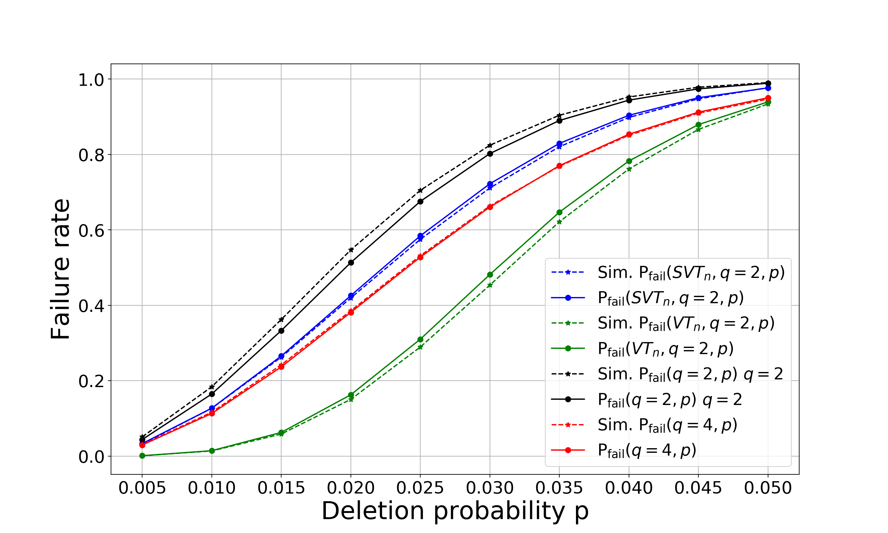
So far we have discussed only the case in which the code is the entire space. However, the most popular deletion-correcting code is theVT code [40]. Recently, SVT, an extension of the VT code has been proposed in [34] for the correction of burst deletions, where the goal of this code construction was to correct a deletion error that its location is known up to some roughly consecutive locations. However, this construction has been recently used in [7] to build a code that is specifically targeted for the reconstruction of a word that is transmitted through two single-deletion channels. Due to the relevance of correcting deletion and alternating errors, the decoding failure probabilities of these two codes is investigated in this work. We abbreviate the notation of by , respectively. The following theorem summarizes these results.
Theorem 10
. The average decoding failure probabilities for the VT and SVT codes are given by
Proof:
The proof follows from the observation that the VT code is capable of decoding either a single run error or a single alternating error. On the other hand, the shifted VT code is capable of only correcting a single alternating error; see [7] for more details. ∎
We verified the theoretical results presented in this section by the following simulations. These simulations were tested over words of length which were used to create two noisy copies given a fixed deletion probability . Then, the two copies were decoded by the ML decoder as described in Claim 4. Finally, we calculated the Levenshtein error rate of the decoded word as well as the average decoding failure probability (referred here as failure rate). Fig. 1 plots the results of the Levenshtein error rate which confirms the probability expression from Theorem 8. Similarly, in Fig. 2 we present separately the error probability , along with the corresponding value as calculated in Lemma 5, 6, respectively. Lastly, in Fig. 3, we simulated the ML decoder for the VT codes and the SVT codes and calculated the failure rate . The implementation of the VT code was taken from [37], and we modified this implementation for SVT codes.


V Two Insertion Channels
This section continues the two-channel study but for for insertion case. In a similar manner to the deletion case, also here the dominant errors result from increasing the length of a run and error that results from the occurrence of an alternating sequence. We denote by the Levenshtein error rate of the ML decoder upon two instances of the insertion channel . Similarly, is the average decoding failure probability and lastly is the insertion probability due to runs, occurrence probability due to alternate sequences, respectively. The following theorem summarizes the results of this section.
Theorem 11
. For the insertion channel , it holds that
Since the proof of this theorem repeats the same ideas as the ones for the deletion case we omit its details here.
The theoretical results of Theorem 11 have also been verified by simulation results over words of length , which were used to create two noisy copies with a given fixed insertion probability . Then, the two copies were decoded with the ML decoder according to Claim 4. Lastly, we calculated and plotted in Fig. 4 the Levenshtein error rate as well as the error rates from runs and alternating sequences.

VI Conclustion
The main contribution of this paper is the study of the decoding error probability of the ML decoder for two deletion or insertion channels. While the results in the paper provide a significant contribution in the area of codes for insertions and deletions and sequence reconstruction, there are still several interesting problems which are left open. Some of them are summarized as follows:
- 1.
Study the non-identical channels case. For example two deletion channels with different probabilities and .
- 2.
Study the decoding error probability for more than two channels, both for insertions and deletions.
- 3.
Study channels which introduce insertions, deletions, and substitutions.
- 4.
Design coding schemes as well as complexity-efficient algorithms for the ML decoder in each case.
References
- [1] M. Abroshan, R. Venkataramanan, L. Dolecek, and A. G. i Fàbregas. Coding for deletion channels with multiple traces. CoRR, abs/1905.08197, 2019.
- [2] L. Anavy, I. Vaknin, O. Atar, R. Amit, and Z. Yakhini. Data storage in dna with fewer synthesis cycles using composite dna letters. Nature biotechnology, 37(10):1229–1236, 2019.
- [3] A. Apostolico, S. Browne, and C. Guerra. Fast linear-space computations of longest common subsequences. Theoretical Computer Science, 92(1):3–17, 1992.
- [4] A. Atashpendar, M. Beunardeau, A. Connolly, R. Géraud, D. Mestel, A. W. Roscoe, and P. Y. A. Ryan. From clustering supersequences to entropy minimizing subsequences for single and double deletions. CoRR, abs/1802.00703, 2018.
- [5] T. Batu, S. Kannan, S. Khanna, and A. McGregor. Reconstructing strings from random traces. In Proceedings of the fifteenth annual ACM-SIAM symposium on Discrete algorithms, pages 910–918. Society for Industrial and Applied Mathematics, 2004.
- [6] A. Blum, T. Jiang, M. Li, J. Tromp, and M. Yannakakis. Linear approximation of shortest superstrings. Journal of the ACM, 41, 12 1993.
- [7] Y. M. Chee, H. M. Kiah, A. Vardy, V. K. Vu, and E. Yaakobi. Coding for racetrack memories. IEEE Transactions on Information Theory, 64(11):7094–7112, Nov 2018.
- [8] Y. Chen, A. Wan, and W. Liu. A fast parallel algorithm for finding the longest common sequence of multiple biosequences. BMC bioinformatics, 7(4):S4, 2006.
- [9] G. M. Church, Y. Gao, and S. Kosuri. Next-generation digital information storage in DNA. Science, 337(6102):1628–1628, 2012.
- [10] A. De, R. O’Donnell, and R. A. Servedio. Optimal mean-based algorithms for trace reconstruction. In Proceedings of the 49th Annual ACM SIGACT Symposium on Theory of Computing, pages 1047–1056. ACM, 2017.
- [11] J. Duda, W. Szpankowski, and A. Grama. Fundamental bounds and approaches to sequence reconstruction from nanopore sequencers. arXiv preprint arXiv:1601.02420, 2016.
- [12] C. Elzinga, S. Rahmann, and H. Wang. Algorithms for subsequence combinatorics. Theoretical Computer Science, 409(3):394–404, 2008.
- [13] R. Gabrys and E. Yaakobi. Sequence reconstruction over the deletion channel. IEEE Transactions on Information Theory, 64(4):2924–2931, 2018.
- [14] R. N. Grass, R. Heckel, M. Puddu, D. Paunescu, and W. J. Stark. Robust chemical preservation of digital information on DNA in silica with error-correcting codes. Angewandte Chemie International Edition, 54(8):2552–2555, 2015.
- [15] D. S. Hirschberg. A linear space algorithm for computing maximal common subsequences. Communications of the ACM, 18(6):341–343, 1975.
- [16] D. S. Hirschberg. Algorithms for the longest common subsequence problem. Journal of the ACM (JACM), 24(4):664–675, 1977.
- [17] N. Holden, R. Pemantle, and Y. Peres. Subpolynomial trace reconstruction for random strings and arbitrary deletion probability. arXiv preprint arXiv:1801.04783, 2018.
- [18] T. Holenstein, M. Mitzenmacher, R. Panigrahy, and U. Wieder. Trace reconstruction with constant deletion probability and related results. In Proceedings of the nineteenth annual ACM-SIAM symposium on Discrete algorithms, pages 389–398. Society for Industrial and Applied Mathematics, 2008.
- [19] W. Hsu and M. Du. Computing a longest common subsequence for a set of strings. BIT Numerical Mathematics, 24(1):45–59, 1984.
- [20] R. W. Irving and C. B. Fraser. Maximal common subsequences and minimal common supersequences. In M. Crochemore and D. Gusfield, editors, Combinatorial Pattern Matching, pages 173–183, Berlin, Heidelberg, 1994. Springer Berlin Heidelberg.
- [21] S. Y. Itoga. The string merging problem. BIT Numerical Mathematics, 21(1):20–30, 1981.
- [22] H. M. Kiah, T. T. Nguyen, and E. Yaakobi. Coding for sequence reconstruction for single edits. In submitted to IEEE International Symposium on Information Theory, arXiv preprint arXiv:2001.01376, 2020.
- [23] V. Levenshtein, E. Konstantinova, E. Konstantinov, and S. Molodtsov. Reconstruction of a graph from 2-vicinities of its vertices. Discrete Applied Mathematics, 156(9):1399–1406, 2008.
- [24] V. I. Levenshtein. Efficient reconstruction of sequences. IEEE Transactions on Information Theory, 47(1):2–22, 2001.
- [25] V. I. Levenshtein. Efficient reconstruction of sequences from their subsequences or supersequences. Journal of Combinatorial Theory, Series A, 93(2):310–332, 2001.
- [26] V. I. Levenshtein and J. Siemons. Error graphs and the reconstruction of elements in groups. Journal of Combinatorial Theory, Series A, 116(4):795–815, 2009.
- [27] W. J. Masek and M. S. Paterson. A faster algorithm computing string edit distances. Journal of Computer and System sciences, 20(1):18–31, 1980.
- [28] M. Mitzenmacher. On the theory and practice of data recovery with multiple versions. In 2006 IEEE International Symposium on Information Theory, pages 982–986, July 2006.
- [29] F. Nazarov and Y. Peres. Trace reconstruction with exp (o (n 1/3)) samples. In Proceedings of the 49th Annual ACM SIGACT Symposium on Theory of Computing, pages 1042–1046. ACM, 2017.
- [30] L. Organick, S. D. Ang, Y.-J. Chen, R. Lopez, S. Yekhanin, K. Makarychev, M. Z. Racz, G. Kamath, P. Gopalan, B. Nguyen, C. N. Takahashi, S. Newman, H.-Y. Parker, C. Rashtchian, K. Stewart, G. Gupta, R. Carlson, J. Mulligan, D. Carmean, G. Seelig, L. Ceze, and K. Strauss. Random access in large-scale DNA data storage. Nature Biotechnology, 36:242 EP –, 02 2018.
- [31] Y. Peres and A. Zhai. Average-case reconstruction for the deletion channel: subpolynomially many traces suffice. In 2017 IEEE 58th Annual Symposium on Foundations of Computer Science (FOCS), pages 228–239. IEEE, 2017.
- [32] F. Sala, R. Gabrys, C. Schoeny, and L. Dolecek. Three novel combinatorial theorems for the insertion/deletion channel. In 2015 IEEE International Symposium on Information Theory (ISIT), pages 2702–2706. IEEE, 2015.
- [33] D. Sankoff. Matching sequences under deletion/insertion constraints. Proceedings of the National Academy of Sciences, 69(1):4–6, 1972.
- [34] C. Schoeny, A. Wachter-Zeh, R. Gabrys, and E. Yaakobi. Codes correcting a burst of deletions or insertions. IEEE Transactions on Information Theory, 63(4):1971–1985, April 2017.
- [35] S. R. Srinivasavaradhan, M. Du, S. Diggavi, and C. Fragouli. On maximum likelihood reconstruction over multiple deletion channels. In 2018 IEEE International Symposium on Information Theory (ISIT), pages 436–440. IEEE, 2018.
- [36] S. R. Srinivasavaradhan, M. Du, S. Diggavi, and C. Fragouli. Symbolwise map for multiple deletion channels. In 2019 IEEE International Symposium on Information Theory (ISIT), pages 181–185. IEEE, 2019.
- [37] K. Tatwawadi and S. Chandak. Tutorial on algebraic deletion correction codes. CoRR, abs/1906.07887, 2019.
- [38] Z. Tronicek. Problems related to subsequences and supersequences. In 6th International Symposium on String Processing and Information Retrieval. 5th International Workshop on Groupware (Cat. No. PR00268), pages 199–205. IEEE, 1999.
- [39] E. Ukkonen. A linear-time algorithm for finding approximate shortest common superstrings. Algorithmica, 5(1-4):313–323, 1990.
- [40] R. R. Varshamov and G. M. Tenenholtz. A code for correcting a single asymmetric error. Automatica i Telemekhanika, 26(2):288–292, 1965.
- [41] E. Yaakobi and J. Bruck. On the uncertainty of information retrieval in associative memories. In 2012 IEEE International Symposium on Information Theory Proceedings, pages 106–110. IEEE, 2012.
- [42] E. Yaakobi, M. Schwartz, M. Langberg, and J. Bruck. Sequence reconstruction for grassmann graphs and permutations. In 2013 IEEE International Symposium on Information Theory, pages 874–878. IEEE, 2013.
- [43] S. H. T. Yazdi, R. Gabrys, and O. Milenkovic. Portable and error-free DNA-based data storage. Scientific Reports, 7(1):5011, 2017.