Structure functions from the Compton amplitude
Abstract:
We have initiated a program to compute the Compton amplitude from lattice QCD with the Feynman-Hellman method. This amplitude is related to the structure function via a Fredholm integral equation of the first kind. It is known that these types of equations are inherently ill–posed - they are, e.g., extremely sensitive to perturbations of the system. We discuss two methods which are candidates to handle these problems: the model free inversion based on singular value decomposition and one Bayesian type approach. We apply the Bayesian method to currently available lattice data for the Compton amplitude.
16-22 June 2019
Wuhan, China
DESY 20-005
ADP-20-3/T1113
LTH-1222
1 Introduction
The determination of the hadronic structure from first principles belongs to the key investigation topics in lattice QCD. Central to our understanding of hadron structure are the structure functions which describe the distribution of quarks and gluons inside hadrons. In the last years some promising approaches have been proposed, among them the calculation of the quasi particle distribution functions (for a review see [1]). Our group has initiated a program to compute the structure functions from the forward Compton amplitude of the nucleon [2, 3]. A central motivation for this is to overcome the issues of renormalization, operator mixing and the restriction to light-cone operators.
The starting point is the forward Compton amplitude of the nucleon [4],
| (1) |
which involves the time ordered product of electromagnetic currents sandwiched between nucleon states of momentum and polarization , where is the momentum of the virtual photon and is the polarization density matrix. In view of our investigation below we consider only the unpolarized structure functions. In the unphysical region () the relation of to the structure functions is given by [4]
| (2) | |||||
with , discarding the subtraction term [2]. To simplify the numerical calculation, we may choose and . We then have
| (3) |
The matrix element can be computed most efficiently by a simple extension of the Feynman–Hellmann method [2, 5].
Performing a Taylor expansion of (3) leads to a simple relation between the moments of the structure function and the –dependent Compton amplitude
| (4) |
From these we then determine the moments of the parton distributions from neglecting logs and terms .
2 Problems and solutions of the Fredholm integral equation
Formula (3) is the basic relation for our investigation. It tells us how to extract the structure function given that we have available lattice data for the Compton amplitude . Unfortunately, it is a Fredholm integral equation of the first kind. Those equations are known to be ill–posed. E.g., they are extremely sensitive to very small perturbations of the data [6] – in our case to the lattice results of . Additionally, the solutions are not guaranteed to be unique. There is no general solution method available. If one finds a successful numerical strategy at all it depends always on the specific kernel . Therefore, a careful study of possible approaches is needed. An analogous problem arises in the reconstruction of Ioffe time pseudo particle distribution functions (pdf) and was investigated in great detail in [7].
In order to test some possible numerical methods we generate mock data for the Compton amplitude. As an example we choose a valence type up quark distribution
| (5) |
chosen to satisfy the momentum sum rule
| (6) |
This function is then used to generate the data via (3) and to compare with the results of our tested inversion algorithms.
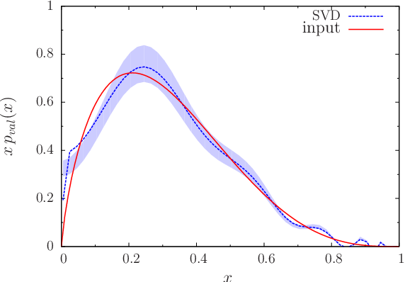
One basic method to solve (7) for the is the singular value decomposition (SVD) [8]. It has the advantage that one does not need to make any further input assumptions about the expected form of the wanted . On the other hand there is a certain freedom in omitting small singular values. Additionally, using our kernel (3) we have cancellations of very large numbers which increases with the number of included singular values. This demands very precise lattice data in order to get meaningful results. The result of the inversion is shown in the left panel of Fig. 1 for , and . One recognizes a trend around the the input distribution with some small oscillations . The integral using the mean value is
An alternative approach uses some prior model information concerning the distribution and tries to refine it according to the available data. It belongs to the class of Bayesian methods. One variant has been discussed in detail in [7]. We follow a slightly different procedure here (see also [3]). Our model assumption is the general form of a valence quark type distribution
| (8) |
We can determine the Compton amplitude from (3) analytically (for )
| (9) | |||||
| (10) |
where is a regularized hypergeometric function. The power expansion of is given in (10). We proceed by first generating Monte Carlo sets of model parameters . With these sets the quadratic deviations
| (11) |
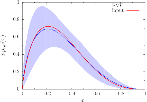
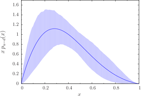
are computed. are the data for , whereas is (2.5) calculated for one triple at . is the inverse covariance matrix of the data. The set is used to make a weighted random choice out of the total set by the likelihood . This constitutes our sample parameter set from which we compute the means and the quantiles. Also in this case the model input is crucial: the final values are inside the MC sets and the should contain reasonable small minimal values. We call this method a Bayesian Monte Carlo (BMC) approach. The resulting distribution is shown in the right panel of Fig. 1. The initial values of the parameters are selected uniformly distributed around some suitable values. An analogous procedure can be used to determine the moments via relation (4). In this case the moments play the role of the parameters and are obtained directly from this approach.
Summarizing the SVD and the BMC approaches we favor the latter, because we recognize in the SVD solution oscillations around the exact result although we use ideal mock data. For real lattice data which are far more scattered and which often have more significant uncertainties the SVD inversion gives very unstable results.
3 First results from lattice data
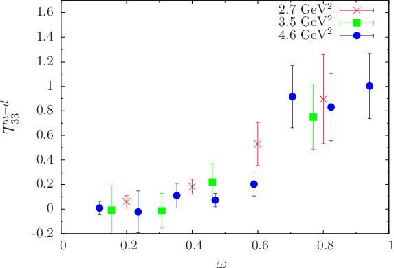
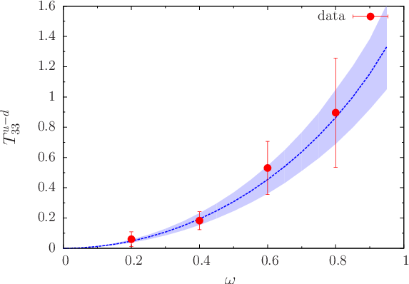
Now we investigate these methods with our latest lattice data for the nucleon Compton amplitude for the connected part of the combination . We use lattices at the SU(3)–flavour symmetric point and GeV. In this paper only data for GeV2 are included. They are shown in the left panel of Fig. 2.

As a first step we determine the first moments using (4) as the defining relation. In this paper we restrict ourselves to order . In order to get information about the –dependence we apply our BMC procedure to each of the three data sets mentioned above. We compute the values from (11), now with
| (12) |
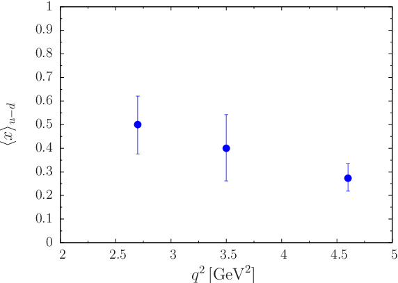
We select sets by sampling uniformly from intervals suggested by phenomenology and determine the moments according to their valence quark beavior. (A random selection with as discussed in [3] leads to very similar results.) We generate 100,000 MC data sets and from that we select a subset of 500 samples weighted by the likelihood . From this subset we compute the . The resulting Compton amplitude is given in the right panel of Fig. 2 for GeV2 where we observe a reasonable agreement with the data. The moments themselves are presented in Fig. 3. They show their expected behavior with increasing order. For the first moment we observe a slight dependence on .

In the same spirit we try to obtain the complete particle distribution function. As data we use the subset with GeV2. Concerning the priors, we are guided by the success of the moments determination above. We sample the first moment uniformly out of the interval and let the BMC method compute it from to the lattice data. This is supported by our model ansatz (8) since
| (13) |
For the parameters and we choose input intervals suggested by phenomenology. Other prior schemes will be investigated in a forthcoming paper.
We find using the mean curve and its quantile borders , consistent with the first moment given in Fig. 3. Additionally, inserting the resulting mean values of the parameters in (10) we find – also compatible with the moments. The results are shown in Fig. 4. One recognizes a strong similarity of the left panel in Fig. 4 with the right panel of Fig. 2 which proves the consistency of both approaches.
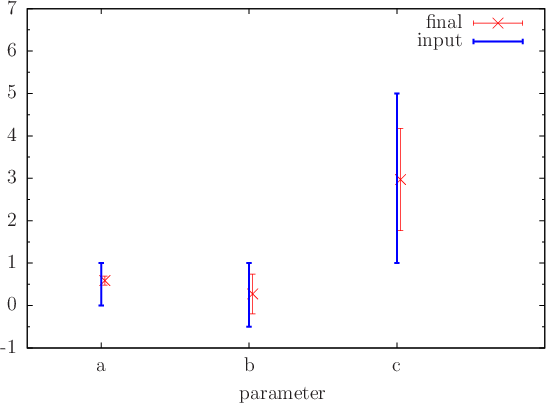
In order to demonstrate the effect of the BMC procedure we show in Fig. 5 the change of the parameters from the uniformly input values (blue) to the final values (red). The histogram in the right panel demonstrates the transition from uniform input to the peaked distribution triggered by the values. One recognizes that the procedure does not influence very much the values of the parameters and but significantly shrinks the range for parameter towards the first moment.

Acknowledgements
The numerical configuration generation (using the BQCD lattice QCD program [9])) and data analysis (using the Chroma software library [10]) was carried out on the IBM BlueGene/Q and HP Tesseract using DIRAC 2 resources (EPCC, Edinburgh, UK), the IBM BlueGene/Q (NIC, Jülich, Germany) and the Cray XC40 at HLRN (The North-German Supercomputer Alliance), the NCI National Facility in Canberra, Australia (supported by the Australian Commonwealth Government) and Phoenix (University of Adelaide). RH was supported by STFC through grant ST/P000630/1. HP was supported by DFG Grant No. PE 2792/2-1. PELR was supported in part by the STFC under contract ST/G00062X/1. GS was supported by DFG Grant No. SCHI 179/8-1. RDY and JMZ were supported by the Australian Research Council Grants DP140103067 and DP190100297. We thank all funding agencies
References
- [1] K. Cichy and M. Constantinou, Adv. High Energy Phys. 2019 (2019) 3036904 [arXiv:1811.07248 [hep-lat]].
- [2] A. J. Chambers et al., Phys. Rev. Lett. 118 (2017) no.24, 242001 [arXiv:1703.01153 [hep-lat]].
- [3] R. D. Young, PoS(LATTICE2019) 278.
- [4] R. Devenish and A. Cooper-Sarkar, Deep Inelastic Scattering, Oxford University Press (2003, Oxford, UK); A.V. Manohar, in Lake Louise 1992, Symmetry and Spin in the Standard Model, p. 1-46 [hep-ph/9204208]; K.-F. Liu, Phys. Rev. D 62 (2000) 074501 [hep-ph/9910306].
- [5] R. Horsley et al. Phys. Lett. B 714 (2012) 312 [arXiv:1205.6410 [hep-lat]]; A.J. Chambers et al. Phys. Rev. D 90 (2014) 014510 [arXiv:1405.3019 [hep-lat]]; A. J. Chambers et al. Phys. Rev. D 92 (2015) no.11, 114517 [arXiv:1508.06856 [hep-lat]]; A. J. Chambers et al. Phys. Rev. D 96 (2017) no.11, 114509 [arXiv:1702.01513 [hep-lat]].
- [6] P. C. Hansen, Inverse Problems 8 (1992) 849.
- [7] J. Karpie, K. Orginos, A. Rothkopf and S. Zafeiropoulos, JHEP 1904 (2019) 057 [arXiv:1901.05408 [hep-lat]].
- [8] W.H. Press, B.P. Flannery, S.A. Teukolsky and W.T. Vetterling, Numerical Recipes, Cambridge University Press (1989, Cambridge, UK).
- [9] T. R. Haar, Y. Nakamura and H. Stüben, EPJ Web Conf. 175 (2018) 14011 [arXiv:1711.03836 [hep-lat]].
- [10] R. G. Edwards et al. [SciDAC and LHPC and UKQCD Collaborations], Nucl. Phys. Proc. Suppl. 140 (2005) 832 [hep-lat/0409003].