跳到论文正文
W Papers独立论文阅读器 arXiv:2001.05344 论文正文 计算阅读时间 · 0%
引用这篇论文根据当前论文元数据生成,正式投稿前建议核对。


License: arXiv.org perpetual non-exclusive license
arXiv:2001.05344v2 [stat.ME] 06 Oct 2020

Nonparametric tests of the causal null
with non-discrete exposures

Ted Westling Note: We are grateful for helpful feedback on this project from Dylan Small, Marco Carone, the University of Pennsylvania Causal Inference Working Group, and three anonymous referees. Affiliation: Department of Mathematics and Statistics Affiliation: University of Massachusetts Amherst Email: twestling@math.umass.edu
Abstract

In many scientific studies, it is of interest to determine whether an exposure has a causal effect on an outcome. In observational studies, this is a challenging task due to the presence of confounding variables that affect both the exposure and the outcome. Many methods have been developed to test for the presence of a causal effect when all such confounding variables are observed and when the exposure of interest is discrete. In this article, we propose a class of nonparametric tests of the null hypothesis that there is no average causal effect of an arbitrary univariate exposure on an outcome in the presence of observed confounding. Our tests apply to discrete, continuous, and mixed discrete-continuous exposures. We demonstrate that our proposed tests are doubly-robust consistent, that they have correct asymptotic type I error if both nuisance parameters involved in the problem are estimated at fast enough rates, and that they have power to detect local alternatives approaching the null at the rate n−1/2n^{-1/2}. We study the performance of our tests in numerical studies, and use them to test for the presence of a causal effect of BMI on immune response in early-phase vaccine trials.

1 Introduction

1.1 Motivation and literature review

One of the central goals of many scientific studies is to determine whether an exposure of interest has a causal effect on an outcome. In some cases, researchers are able to randomly assign units to exposure values. Classical statistical methods for assessing the association between two random variables can then be used to determine whether there is a causal effect because randomization ensures that there are no common causes of the exposure and the outcome. However, random assignment of units to exposures is not feasible in some settings, and even when it is feasible, preliminary evidence is often needed to justify a randomized study. In either case, it is often of interest to use data from an observational study, in which the exposure is not assigned by the researcher but instead varies according to some unknown mechanism, to assess the evidence of a causal effect. This is a more difficult task due to potential confounding of the exposure-outcome relationship.

Here, we are interested in assessing whether a non-randomized exposure that occurs at a single time point has a causal effect on a subsequent outcome when it can be assumed that there are no unobserved confounders. Many methods have been proposed to test the null hypothesis that there is no causal effect in this setting when the exposure is discrete. For instance, matching estimators (Rubin 1973), inverse probability weighted (IPW) estimators (Horvitz and Thompson 1952), and doubly-robust estimators including augmented IPW (Scharfstein et al. 1999; Bang and Robins 2005) and targeted minimum loss-based estimators (TMLE) (van der Laan and Rose 2011) can all be used for this purpose.

Much less work exists in the context of non-discrete exposures—that is, exposures that may take an uncountably infinite number of values. In practice, researchers often discretize such an exposure in order to return to the discrete exposure setting. This simple approach has several drawbacks. First, since the results often vary with the choice of discretization, it may be tempting for researchers to choose a discretization based on the results. However, this can inflate type I error rate. Second, tests based on a discretized exposure typically have less power than tests based on the original exposure because discretizing discards possibly relevant information (see, e.g. Cox 1957; Cohen 1983; Fedorov et al. 2009). Finally, causal estimates based on a discretized exposure have a more complicated interpretation than those based on the original exposure (Young et al. 2019).

In the context of causal inference with a continuous exposure, one common estimand is the causal dose-response curve, which is defined for each value of the exposure as the average outcome were all units assigned to that exposure value. We say there is no average causal effect if the dose-response curve is flat; i.e. the average outcome does not depend on the assigned value of the exposure. One approach to estimating the dose-response curve is to assume the regression of the outcome on the exposure and confounders follows a linear model. If the model is correctly specified, the coefficient corresponding to the exposure is the slope of the dose-response curve, and the null hypothesis that the dose-response curve is flat can be assessed by testing whether this coefficient is zero. This approach can be generalized to other regression models, which can be marginalized using the G-formula to obtain the dose-response function (Robins 1986; Robins 2000; Zhang et al. 2016). However, if the regression model is mis-specified, then the resulting estimator of the causal dose-response curve is typically inconsistent, and the resulting test will not necessarily be calibrated or consistent. Inverse probability weighting may also be used to estimate the dose-response curve (Imai and van Dyk 2004; Hirano and Imbens 2005), but mis-specification of the propensity score model may again lead to unreliable inference.

Nonparametric methods make fewer assumptions about the data-generating mechanism than methods based on parametric models, and are therefore often more robust. In the context of nonparametric estimation of a causal dose-response curve, Neugebauer and van der Laan 2007 considered inference for the projection onto a parametric working model; Rubin and van der Laan 2006 and Díaz and van der Laan 2011 discussed the use of data-adaptive algorithms; Kennedy et al. 2017 and van der Laan et al. 2018 proposed estimators based on kernel smoothing; and Westling et al. 2020 proposed an isotonic estimator. However, none of these works considered tests of the null hypothesis that the dose-response curve is flat. We also note that tests of Granger causality (Granger 1980) have been developed in the context of time series (e.g. Granger and Lin 1995; Boudjellaba et al. 1992; Nishiyama et al. 2011). This is distinct from our goal, which is to test whether an exposure at a single time point has a causal effect on the average of a subsequent outcome.

1.2 Contribution and organization of the article

In this article, we focus on the problem of testing the null hypothesis that there is no average causal effect of a possibly non-discrete exposure on an outcome against the complementary alternative. To the best of our knowledge, no nonparametric test has yet been developed for this purpose. Specifically, we (1) propose a test based on a cross-fitted nonparametric estimator of an integral of the causal dose-response curve; (2) provide conditions under which our test has desirable large-sample properties, including (i) consistency under any alternative as long as either of two nuisance functions involved in the problem is estimated consistently (known as doubly-robust consistency), (ii) asymptotically correct type I error rate, and (iii) non-zero power under local alternatives approaching the null at the rate n−1/2n^{-1/2}; and (3) illustrate the practical performance of the tests through numerical studies and an analysis of the causal effect of BMI on immune response in early-phase vaccine trials.

Notably, the conditions we establish for consistency and validity of our test do not restrict the form of the marginal distribution of the exposure. Therefore, our test applies equally to discrete, continuous, and mixed discrete-continuous exposures. In the second set of numerical studies, we demonstrate that even in the context of discrete exposures, existing tests do not control type I error when the number of discrete components is moderate or large relative to sample size, while the tests proposed here are valid in all such circumstances.

The remainder of the article is organized as follows. In Section 2, we define our proposed procedure. In Section 3, we discuss the large-sample properties of our procedure. In Section 4, we illustrate the behavior of our method using numerical studies. In Section Additional results from analysis of the effect of BMI on immune response, we use our procedure to analyze the causal effect of BMI on immune response. Section 6 presents a brief discussion. Proofs of all theorems are provided in Supplementary Material. An R (R Core Team 2020) package implementing all the methods developed in this paper is available at https://github.com/tedwestling/ctsCausal.

2 Proposed methodology

2.1 Notation and null hypothesis of interest

We denote by A∈𝒜A\in\mathscr{A} the real-valued exposure of interest, whose support we denote by 𝒜0⊆ℝ\mathscr{A}_{0}\subseteq\mathbb{R}. Adopting the Neyman-Rubin potential outcomes framework, for each a∈𝒜0a\in\mathscr{A}_{0}, we denote by Y⁡(a)∈𝒴⊆ℝY(a)\in\mathscr{Y}\subseteq\mathbb{R} a unit’s potential outcome under an intervention setting exposure to A=aA=a. The causal parameter m⁡(a):=E⁡[Y⁡(a)]m(a):=E\left[Y(a)\right] represents the average outcome under assignment of the entire population to exposure level A=aA=a. The resulting curve m:𝒜→ℝm:\mathscr{A}\rightarrow\mathbb{R} is known as the causal dose-response curve.

We are interested in testing the null hypothesis that m⁡(a)=γ0m(a)=\gamma_{0} for all a∈𝒜0a\in\mathscr{A}_{0} and some γ0∈ℝ\gamma_{0}\in\mathbb{R}; that is, the dose-response curve is flat. This null hypothesis holds if and only if the average value of the potential outcome is unaffected by the value of the exposure to which units are assigned. However, Y⁡(a)Y(a) is not typically observed for all units in the population, but instead the outcome Y:=Y⁡(A)Y:=Y(A) corresponding to the exposure value actually received is observed. Thus, mm is not a mapping of the joint distribution of the pair (A,Y)(A,Y), so the null hypothesis that mm is flat cannot be tested using this data. The first step in developing a testing procedure is to translate the causal problem into a problem that is testable with the observed data, which is called identification in the causal inference literature.

We first assume that (i) each unit’s potential outcomes are independent of all other units’ exposures and (ii) the observed outcome YY almost surely equals Y⁡(A)Y(A). If (i)–(ii) hold and in addition (iii) Y⁡(a)⟂⁣⟂AY(a)\mathchoice{\mathrel{\hbox to0.0pt{$\displaystyle\perp$\hss}\mkern 2.0mu{\displaystyle\perp}}}{\mathrel{\hbox to0.0pt{$\textstyle\perp$\hss}\mkern 2.0mu{\textstyle\perp}}}{\mathrel{\hbox to0.0pt{$\scriptstyle\perp$\hss}\mkern 2.0mu{\scriptstyle\perp}}}{\mathrel{\hbox to0.0pt{$\scriptscriptstyle\perp$\hss}\mkern 2.0mu{\scriptscriptstyle\perp}}}A for all a∈𝒜0a\in\mathscr{A}_{0}, then m⁡(a)=E⁡[Y∣A=a]m(a)=E[Y\mid A=a] for all a∈𝒜0a\in\mathscr{A}_{0}. In this case, mm is identified with a univariate regression function, so the null hypothesis that mm is flat on 𝒜0\mathscr{A}_{0} can be tested using existing work from the nonparametric regression literature (see, e.g. Eubank and Spiegelman 1990; Andrews 1997; Horowitz and Spokoiny 2001, among many others). However, assumption (iii) typically only holds in experiments in which AA is randomly assigned. In observational studies, there are typically confounding variables that impact both AA and Y⁡(a)Y(a), thus invalidating (iii). In these settings, tests based on nonparametric regression may not have valid type I error rate, even asymptotically.

We suppose that a collection W∈𝒲⊆ℝpW\in\mathscr{W}\subseteq\mathbb{R}^{p} of possible confounders is recorded. If (i)–(ii) hold and in addition (iv) Y⁡(a)⟂⁣⟂A|WY(a)\mathchoice{\mathrel{\hbox to0.0pt{$\displaystyle\perp$\hss}\mkern 2.0mu{\displaystyle\perp}}}{\mathrel{\hbox to0.0pt{$\textstyle\perp$\hss}\mkern 2.0mu{\textstyle\perp}}}{\mathrel{\hbox to0.0pt{$\scriptstyle\perp$\hss}\mkern 2.0mu{\scriptstyle\perp}}}{\mathrel{\hbox to0.0pt{$\scriptscriptstyle\perp$\hss}\mkern 2.0mu{\scriptscriptstyle\perp}}}A\mid W for all a∈𝒜0a\in\mathscr{A}_{0}, known as no unmeasured confounding, and (v) all a∈𝒜0a\in\mathscr{A}_{0} are in the support of the conditional distribution of AA given W=wW=w for almost every ww, known as positivity, then m⁡(a)=θ0​(a):=E⁡[E⁡(Y∣A=a,W)]m(a)=\theta_{0}(a):=E[E(Y\mid A=a,W)], which is known as the G-computed regression function (Robins 1986; Gill and Robins 2001). Therefore, under (i)–(ii) and (iv)–(v), mm is flat on 𝒜0\mathscr{A}_{0} if and only if θ0\theta_{0} is flat on 𝒜0\mathscr{A}_{0}.

Here, we assume that we observe independent and identically distributed random vectors (Y1,A1,W1),…,(Yn,An,Wn)(Y_{1},A_{1},W_{1}),\dotsc,(Y_{n},A_{n},W_{n}) from a distribution P0P_{0} contained in the nonparametric model ℳN​P\mathscr{M}_{NP} consisting of all distributions on 𝒴×𝒜×𝒲\mathscr{Y}\times\mathscr{A}\times\mathscr{W}. For a distribution P∈ℳN​PP\in\mathscr{M}_{NP}, we denote by FPF_{P} the marginal distribution of AA under PP, 𝒜P\mathscr{A}_{P} the support of FPF_{P}, μP(a,w):=EP[Y∣A=a,W=w]\mu_{P}(a,w):=E_{P}[Y\mid A=a,W=w] the outcome regression function, and QPQ_{P} the marginal distribution of WW. Throughout, we use the subscript 00 to refer to evaluation at or under P0P_{0}; for example, we denote by F0F_{0} the marginal distribution function of AA under P0P_{0} and by 𝒜0\mathscr{A}_{0} the support of F0F_{0}. Denoting by Cb​(S)C_{b}(S) the class of continuous and bounded functions on a subset SS of ℝ\mathbb{R}, we assume that P0P_{0} is contained in the statistical model ℳ:={P∈ℳN​P:θP∈Cb​(𝒜P)}\mathscr{M}:=\{P\in\mathscr{M}_{NP}:\theta_{P}\in C_{b}(\mathscr{A}_{P})\}.

In this article, we focus on testing the null hypothesis H0:P0∈ℳ0⊂ℳH_{0}:P_{0}\in\mathscr{M}_{0}\subset\mathscr{M} for ℳ0:={P∈ℳ:θP(a)=θP(a′) for all a,a′∈𝒜P}\mathscr{M}_{0}:=\left\{P\in\mathscr{M}:\theta_{P}(a)=\theta_{P}(a^{\prime})\text{ for all }a,a^{\prime}\in\mathscr{A}_{P}\right\} versus the complementary alternative HA:P0∈ℳA:=ℳ\ℳ0H_{A}:P_{0}\in\mathscr{M}_{A}:=\mathscr{M}\backslash\mathscr{M}_{0}. This null hypothesis holds if and only if θ0​(a)=γ0\theta_{0}(a)=\gamma_{0} for all a∈𝒜0a\in\mathscr{A}_{0}, where γ0:=∫θ0​(a)​F0​(𝑑a)=∬μ0​(a,w)​Q0​(𝑑w)​F0​(𝑑a)\gamma_{0}:=\int\theta_{0}(a)\,F_{0}(da)=\iint\mu_{0}(a,w)\,Q_{0}(dw)\,F_{0}(da). As noted above, conditions (i)–(ii) and (iv)–(v) imply that H0H_{0} holds if and only if the exposure has no causal effect on the average outcome in the sense that setting AA to aa for all units in the population yields the same average outcome for all a∈𝒜0a\in\mathscr{A}_{0}. On the other hand, HAH_{A} holds if and only if at least two exposures in 𝒜0\mathscr{A}_{0} yield different average outcomes. Our null hypothesis is stated in terms of the possibly unknown 𝒜0\mathscr{A}_{0} because condition (v) does not hold for a∉𝒜0a\notin\mathscr{A}_{0}, and in fact m⁡(a)m(a) is not identified in the observed data for such aa without further assumptions.

A special case of our null hypothesis is that μ0​(a,w)=μ0​(a′,w)\mu_{0}(a,w)=\mu_{0}(a^{\prime},w) for all a,a′∈𝒜0a,a^{\prime}\in\mathscr{A}_{0} and almost all ww. In this case, γ0=E0​[Y]\gamma_{0}=E_{0}[Y]. Under conditions (i)–(ii) and (iv)–(v), this happens if and only if E0​[Y⁡(a)∣W=w]=E0​[Y⁡(a′)∣W=w]E_{0}[Y(a)\mid W=w]=E_{0}[Y(a^{\prime})\mid W=w] for almost all ww—i.e. there is no effect of the exposure on the average potential outcome for any strata of WW in the population. We shall refer to this case as the strong null hypothesis. We emphasize that our null hypothesis H0H_{0} can hold even if the strong null does not, since interactions between the exposure and covariates may average out to yield a flat G-computed regression curve. We note that Luedtke et al. 2019 recently proposed a general procedure for testing null hypotheses of the form R0​(O)=dS0​(O)R_{0}(O)\stackrel{{\scriptstyle d}}{{=}}S_{0}(O), where the generic observation OO follows distribution P0P_{0}, and the functions R0R_{0} and S0S_{0} may depend on P0P_{0}. Luedtke et al. 2019 demonstrated that their procedure can be used to consistently test the strong null hypothesis stated above, albeit with type I error rate tending to zero. Our null hypothesis may also be stated in their general form with R0​(Y,A,W):=θ0​(A)R_{0}(Y,A,W):=\theta_{0}(A) and S0​(Y,A,W):=γ0S_{0}(Y,A,W):=\gamma_{0}. However, their results do not apply to our null hypothesis because their Condition 3 does not hold for R0=θ0R_{0}=\theta_{0}.

For a measure λ\lambda, we define ‖h‖λ,p:=[∫|h⁡(x)|p​𝑑λ​(x)]1/p\|h\|_{\lambda,p}:=\left[\int|h(x)|^{p}\,d\lambda(x)\right]^{1/p} for p∈[1,∞)p\in[1,\infty), and ‖h‖λ,∞:=supx∈supp⁡(λ)|h⁡(x)|\|h\|_{\lambda,\infty}:=\sup_{x\in\mathrm{supp}(\lambda)}|h(x)|. For a probability measure PP and PP-integrable function hh, we define P​h:=∫h​𝑑PPh:=\int h\,dP. We define ℙn\mathbb{P}_{n} as the empirical distribution function of the observed data.

2.2 Testing in terms of the primitive function

Our procedure will be based on estimating a primitive parameter (i.e. an integral) of θ0\theta_{0}. A useful analogy to consider is testing that a density function hh is flat on [0,1][0,1]. A density function, like θ0\theta_{0}, is a challenging parameter to estimate in a nonparametric model, and the fastest attainable rate is slower than n−1/2n^{-1/2}. However, hh is flat if and only if the corresponding cumulative distribution function HH, which is the primitive of hh, is the identity function on [0,1][0,1], which is further equivalent to H⁡(x)−x=0H(x)-x=0 for all x∈[0,1]x\in[0,1]. In our setting, we define the primitive function as Γ0​(a):=∫−∞aθ0​(u)​d​F0​(u)\Gamma_{0}(a):=\int_{-\infty}^{a}\theta_{0}(u)\,dF_{0}(u). We integrate against the marginal distribution F0F_{0} of AA because θ0\theta_{0} is only estimable on the support of F0F_{0}. We then note that θ0​(a)=γ0\theta_{0}(a)=\gamma_{0} for all a∈𝒜0a\in\mathscr{A}_{0} if and only if Γ0​(a)=∫−∞aγ0​d​F0​(u)=γ0​F​(a)\Gamma_{0}(a)=\int_{-\infty}^{a}\gamma_{0}\,dF_{0}(u)=\gamma_{0}F(a). Therefore, our null hypothesis is equivalent to Ω0​(a):=Γ0​(a)−γ0​F0​(a)\Omega_{0}(a):=\Gamma_{0}(a)-\gamma_{0}F_{0}(a) equals 00 for all a∈𝒜0a\in\mathscr{A}_{0}. This is stated formally in the following result.

Proposition 1.

If θ0\theta_{0} is continuous on 𝒜0\mathscr{A}_{0}, then the following are equivalent: (1) P0∈ℳ0P_{0}\in\mathscr{M}_{0}; (2) θ0​(a)=γ0\theta_{0}(a)=\gamma_{0} for all a∈𝒜0a\in\mathscr{A}_{0}; (3) Ω0​(a)=0\Omega_{0}(a)=0 for all a∈ℝa\in\mathbb{R}; (4) ‖Ω0‖F0,p=0\|\Omega_{0}\|_{F_{0},p}=0 for all p≥1p\geq 1.

Refer to caption
Figure 1: Four hypothetical dose-response curves θ⁡(a)\theta(a) (left) and their corresponding primitives Ω⁡(a)\Omega(a) (right). The marginal distribution of the exposure is the standard normal.

For illustrative purposes, Figure 1 displays four hypothetical θ0\theta_{0}’s and their corresponding Ω0\Omega_{0}’s. We note that Ω0​(a)=0\Omega_{0}(a)=0 for all a∈ℝa\in\mathbb{R} if and only if Ω0​(a)=0\Omega_{0}(a)=0 for all a∈𝒜0a\in\mathscr{A}_{0}. This, combined with Proposition 1, indicates that in the model ℳ\mathscr{M}, testing H0H_{0} is equivalent to testing the null hypothesis ‖Ω0‖F0,p=0\|\Omega_{0}\|_{F_{0},p}=0 versus the alternative ‖Ω0‖F0,p>0\|\Omega_{0}\|_{F_{0},p}>0. In the case of testing uniformity of a density, this is analogous to testing that ‖H−Id‖[0,1],p=0\|H-\mathrm{Id}\|_{[0,1],p}=0 for Id⁡(x)=x\mathrm{Id}(x)=x the identity map, which is exactly what the Kolmogorov-Smirnov (in which p=∞p=\infty) and Anderson-Darling (in which p=2p=2) tests do. Furthermore, representing the problem as a test that ‖H−Id‖[0,1],p=0\|H-\mathrm{Id}\|_{[0,1],p}=0 is useful because HH is staightforward to estimate at the n−1/2n^{-1/2} rate, unlike a density function. In our case, Ω0\Omega_{0} is pathwise differentiable in the nonparametric model with an estimable influence function under standard conditions, unlike θ0\theta_{0}. Specifically, defining g0​(a,w):=G0​(d​a,w)/F0​(d​a)g_{0}(a,w):=G_{0}(da,w)/F_{0}(da), where G0​(a,w):=P0​(A≤a∣W=w)G_{0}(a,w):=P_{0}(A\leq a\mid W=w) is the conditional distribution of AA given W=wW=w evaluated at aa, we have the following result.

Proposition 2.

For each a0∈ℝa_{0}\in\mathbb{R}, Ω0​(a0)\Omega_{0}(a_{0}) is pathwise differentiable relative to the subset of ℳ\mathscr{M} in which gPg_{P} is almost surely bounded away from zero and EP​[Y2]<∞E_{P}\left[Y^{2}\right]<\infty, and its efficient influence function is

Da0,0∗​(y,a,w)\displaystyle D_{a_{0},0}^{*}(y,a,w) :=[I(−∞,a0](a)−F0(a0)][y−μ0​(a,w)g0​(a,w)+θ0(a)−γ0]\displaystyle:=\left[I_{(-\infty,a_{0}]}(a)-F_{0}(a_{0})\right]\left[\frac{y-\mu_{0}(a,w)}{g_{0}(a,w)}+\theta_{0}(a)-\gamma_{0}\right]
+∫[I(−∞,a0](u)−F0(a0)]μ0(u,w)F0(du)−2Ω0(a0).\displaystyle\qquad+\int\left[I_{(-\infty,a_{0}]}(u)-F_{0}(a_{0})\right]\mu_{0}(u,w)\,F_{0}(du)-2\Omega_{0}(a_{0})\ .

We note that g0​(a,w)=P0​(A=a∣W=w)/P0​(A=a)g_{0}(a,w)=P_{0}(A=a\mid W=w)/P_{0}(A=a) for aa such that P0​(A=a)>0P_{0}(A=a)>0, and g0​(a,w)=[dd​a​P0​(A≤a∣W=w)]/[dd​a​F0​(a)]g_{0}(a,w)=\left[\frac{d}{da}P_{0}(A\leq a\mid W=w)\right]/\left[\frac{d}{da}F_{0}(a)\right] for aa where F0F_{0} is absolutely continuous. Hence, g0g_{0} generalizes both the standardized generalized propensity score (GPS) and the standardized propensity score.

For any p∈[1,∞]p\in[1,\infty], Proposition 2 allows us to test H0H_{0} in the following manner: (1) construct a uniformly asymptotically linear estimator Ωn∘\Omega_{n}^{\circ} of Ω0\Omega_{0} for which {n1/2​[Ωn∘​(a)−Ω0​(a)]:a∈𝒜0}\{n^{1/2}[\Omega_{n}^{\circ}(a)-\Omega_{0}(a)]:a\in\mathscr{A}_{0}\} converges weakly to a Gaussian limit process, (2) use the estimated influence function of Ωn∘​(a)\Omega_{n}^{\circ}(a) to construct an estimator Tn,p,αT_{n,p,\alpha} of the 1−α1-\alpha quantile of n1/2​‖Ωn∘−Ω0‖F0,pn^{1/2}\|\Omega_{n}^{\circ}-\Omega_{0}\|_{F_{0},p}, and (3) reject H0H_{0} at level α\alpha if n1/2​‖Ωn∘‖Fn,p>Tn,p,αn^{1/2}\|\Omega_{n}^{\circ}\|_{F_{n},p}>T_{n,p,\alpha}. In the remainder of this section, we provide details for accomplishing each of these three steps.

2.3 Estimating the primitive function

The first step in our testing procedure is to construct an asymptotically linear estimator of Ω0​(a)\Omega_{0}(a) for each fixed aa. The four nuisance parameters present in the definition of Ω0​(a0)\Omega_{0}(a_{0}) and its nonparametric efficient influence function Da0,0∗D_{a_{0},0}^{*} are the outcome regression μ0\mu_{0}, the standardized propensity g0g_{0}, and the marginal distributions F0F_{0} and Q0Q_{0} corresponding to AA and WW, respectively. Given estimators μn\mu_{n} and gng_{n} of μ0\mu_{0} and g0g_{0}, respectively, we can construct an estimator Da0,n∗D_{a_{0},n}^{*} of the influence function by plugging in μn\mu_{n} for μ0\mu_{0}, gng_{n} for g0g_{0}, and the empirical marginal distributions FnF_{n} and QnQ_{n} for F0F_{0} and Q0Q_{0}. A one-step estimator of Ω0​(a0)\Omega_{0}(a_{0}) is then given by Ωn​(a0):=Ωμn,Fn,Qn​(a0)+ℙn​Da0,n∗\Omega_{n}(a_{0}):=\Omega_{\mu_{n},F_{n},Q_{n}}(a_{0})+\mathbb{P}_{n}D_{a_{0},n}^{*}, where Ωμn,Fn,Qn(a0):=∬[I(−∞,a0](a)−Fn(a0)]μn(a,w)dFn(a)dQn(w)\Omega_{\mu_{n},F_{n},Q_{n}}(a_{0}):=\iint\left[I_{(-\infty,a_{0}]}(a)-F_{n}(a_{0})\right]\mu_{n}(a,w)\,dF_{n}(a)\,dQ_{n}(w) is the plug-in estimator of Ω0\Omega_{0}. In expanding Ωn​(a0)\Omega_{n}(a_{0}), some terms cancel and we are left with

Ωn(a0)=1n∑i=1n[I(−∞,a0](Ai)−Fn(a0)][Yi−μn​(Ai,Wi)gn​(Ai,Wi)+∫μn(Ai,w)dQn(w)].\Omega_{n}(a_{0})=\frac{1}{n}\sum_{i=1}^{n}\left[I_{(-\infty,a_{0}]}(A_{i})-F_{n}(a_{0})\right]\left[\frac{Y_{i}-\mu_{n}(A_{i},W_{i})}{g_{n}(A_{i},W_{i})}+\int\mu_{n}(A_{i},w)\,dQ_{n}(w)\right]\ . (1)

If we were to base our test on Ωn\Omega_{n}, then, as we will see in Section 3, the large-sample properties of our test would depend on consistency of Ωn\Omega_{n} and on weak convergence of {n1/2​[Ωn​(a)−Ω0​(a)]:a∈𝒜0}\{n^{1/2}[\Omega_{n}(a)-\Omega_{0}(a)]:a\in\mathscr{A}_{0}\} as a process. Such statistical properties of asymptotically linear estimators of pathwise differentiable parameters depend on estimators of nuisance parameters in two important ways. First, negligibility of a so-called second-order remainder term requires negligibility of (μn−μ0)​(gn−g0)(\mu_{n}-\mu_{0})(g_{n}-g_{0}) in an appropriate sense. Second, negligibility of empirical process remainder terms can be guaranteed if the nuisance estimators fall in sufficiently small function classes. In observational studies, researchers can rarely specify a priori correct parametric models for μ0\mu_{0} or g0g_{0}, which motivates the use of data-adaptive (e.g. machine learning) estimation of these functions in order to achieve negligibility of the second-order remainder. However, data-adaptive estimators typically constitute large function classes. Hence, finding estimators that simultaneously satisfy these two requirements can require a delicate balance. Cross-fitting has been found to resolve this challenge by removing the need for nuisance estimators to fall in small function classes (Zheng and van der Laan 2011; Belloni et al. 2018; Kennedy 2019). Instead of basing our test on Ωn\Omega_{n}, we will therefore base our test on a cross-fitted version of Ωn\Omega_{n}, which we now define.

For a deterministic integer V∈{2,3,…,⌊n/2⌋}V\in\{2,3,\dotsc,\lfloor n/2\rfloor\}, we randomly partition the indices {1,…,n}\{1,\dotsc,n\} into VV disjoint sets 𝒱n,1,…,𝒱n,V\mathscr{V}_{n,1},\dotsc,\mathscr{V}_{n,V} with cardinalities N1,…,NVN_{1},\dotsc,N_{V}. We require that these sets be as close to equal sizes as possible, so that |Nv−n/V|≤1|N_{v}-n/V|\leq 1 for each vv, and that the number of folds VV be bounded as nn grows. For each v∈{1,…,V}v\in\{1,\dotsc,V\}, we define 𝒯n,v:={Oi:i∉𝒱n,v}\mathscr{T}_{n,v}:=\{O_{i}:i\notin\mathscr{V}_{n,v}\} as the training set for fold vv, and we define μn,v\mu_{n,v} and gn,vg_{n,v} as nuisance estimators that are estimated using only the observations from 𝒯n,v\mathscr{T}_{n,v}. Similarly, we define Fn,vF_{n,v} and Qn,vQ_{n,v} as the marginal empirical distributions of AA and WW, respectively, corresponding to the observations in 𝒯n,v\mathscr{T}_{n,v}. We then define the cross-fitted estimator Ωn∘\Omega_{n}^{\circ} of Ω0\Omega_{0} as

Ωn∘​(a0)\displaystyle\Omega_{n}^{\circ}(a_{0}) :=1V∑v=1V{1Nv∑i∈𝒱n,v[I(−∞,a0](Ai)−Fn,v(a0)]Yi−μn,v​(Ai,Wi)gn,v​(Ai,Wi)\displaystyle:=\frac{1}{V}\sum_{v=1}^{V}\left\{\frac{1}{N_{v}}\sum_{i\in\mathscr{V}_{n,v}}\left[I_{(-\infty,a_{0}]}(A_{i})-F_{n,v}(a_{0})\right]\frac{Y_{i}-\mu_{n,v}(A_{i},W_{i})}{g_{n,v}(A_{i},W_{i})}\right.
+1Nv2∑i,j∈𝒱n,v[I(−∞,a0](Ai)−Fn,v(a0)]μn,v(Ai,Wj)}.\displaystyle\qquad\qquad\qquad\left.+\frac{1}{N_{v}^{2}}\sum_{i,j\in\mathscr{V}_{n,v}}\left[I_{(-\infty,a_{0}]}(A_{i})-F_{n,v}(a_{0})\right]\mu_{n,v}(A_{i},W_{j})\right\}\ . (2)

In the next section, we indicate properties of the estimators μn,v\mu_{n,v} and gn,vg_{n,v} that imply certain large-sample properties of Ωn∘\Omega_{n}^{\circ}, which in turn imply properties of our testing procedure. In particular, we provide conditions under which Ωn∘​(a)\Omega_{n}^{\circ}(a) is uniformly asymptotically linear with influence function Da,0∗D_{a,0}^{*}, meaning that

Ωn∘​(a)−Ω0​(a)=ℙn​Da,0∗+Rn​(a),\Omega_{n}^{\circ}(a)-\Omega_{0}(a)=\mathbb{P}_{n}D_{a,0}^{*}+R_{n}(a)\ , (3)

where supa∈𝒜0|Rn(a)|=oP0(n−1/2)\sup_{a\in\mathscr{A}_{0}}|R_{n}(a)|=o_{P_{0}}(n^{-1/2}). If (3) holds and in addition the one-dimensional class of functions {Da,0∗:a∈𝒜0}\{D_{a,0}^{*}:a\in\mathscr{A}_{0}\} is P0P_{0}-Donsker, then {n1/2​[Ωn∘​(a)−Ω0​(a)]:a∈𝒜0}\{n^{1/2}[\Omega_{n}^{\circ}(a)-\Omega_{0}(a)]:a\in\mathscr{A}_{0}\} converges weakly in the space ℓ∞​(𝒜0)\ell^{\infty}(\mathscr{A}_{0}) of bounded real-valued functions on 𝒜0\mathscr{A}_{0} to a mean-zero Gaussian process Z0Z_{0} with covariance function Σ0​(s,t):=P0​[Ds,0∗​Dt,0∗]\Sigma_{0}(s,t):=P_{0}[D_{s,0}^{*}D_{t,0}^{*}]. Since the Lp​(F0)L_{p}(F_{0})-norm is a continuous functional on ℓ∞​(𝒜0)\ell^{\infty}(\mathscr{A}_{0}) for any p∈[1,∞]p\in[1,\infty], by the continuous mapping theorem we will then have n1/2∥Ωn∘−Ω0∥F0,p⟶d∥Z0∥F0,pn^{1/2}\|\Omega_{n}^{\circ}-\Omega_{0}\|_{F_{0},p}\indist\|Z_{0}\|_{F_{0},p}. Given an estimator Da,n,v∗D_{a,n,v}^{*} of Da,0∗D_{a,0}^{*} for each vv, we can approximate the distribution ‖Z0‖F0,p\|Z_{0}\|_{F_{0},p} by simulating sample paths of a mean-zero Gaussian process ZnZ_{n} with covariance function Σn​(s,t):=1V​∑v=1Vℙn,v​Ds,n,v∗​Dt,n,v∗\Sigma_{n}(s,t):=\frac{1}{V}\sum_{v=1}^{V}\mathbb{P}_{n,v}D_{s,n,v}^{*}D_{t,n,v}^{*}, and computing the Lp​(Fn)L_{p}(F_{n})-norm of these sample paths, where ℙn,v\mathbb{P}_{n,v} is the empirical distribution for the validation fold 𝒱n,v\mathscr{V}_{n,v}. Putting it all together, our fully specified procedure for testing the null hypotheses H0H_{0} is as follows:

Step 1:

Split the sample into VV sets 𝒱n,1,…,𝒱n,V\mathscr{V}_{n,1},\dotsc,\mathscr{V}_{n,V} of approximately equal size.

Step 2:

For each v∈{1,…,V}v\in\{1,\dotsc,V\}, construct estimates μn,v\mu_{n,v} and gn,vg_{n,v} of the nuisance functions μ0\mu_{0} and g0g_{0} based on the training set 𝒯n,v\mathscr{T}_{n,v} for fold vv.

Step 3:

For each aa in the observed values of the exposure 𝒜n:={A1,…,An}\mathscr{A}_{n}:=\{A_{1},\dotsc,A_{n}\}, use μn,v\mu_{n,v} and gn,vg_{n,v} to construct Ωn∘​(a)\Omega_{n}^{\circ}(a) as defined in (2).

Step 4:

Let Tn,α,pT_{n,\alpha,p} be the 1−α1-\alpha quantile of (1n​∑i=1n|Zn​(Ai)|p)1/p\left(\frac{1}{n}\sum_{i=1}^{n}|Z_{n}(A_{i})|^{p}\right)^{1/p} for p<∞p<\infty or maxa∈𝒜n⁡|Zn​(Ai)|\max_{a\in\mathscr{A}_{n}}|Z_{n}(A_{i})| for p=∞p=\infty, where, conditional on O1,…,OnO_{1},\dotsc,O_{n}, (Zn​(A1),…,Zn​(An))(Z_{n}(A_{1}),\dotsc,Z_{n}(A_{n})) is distributed according to a mean-zero multivariate normal distribution with covariances given by Σn(Ai,Aj):=E[Zn(Ai)Zn(Aj)∣O1,…,On]=1V∑v=1Vℙn,vDAi,n,v∗DAj,n,v∗\Sigma_{n}(A_{i},A_{j}):=E[Z_{n}(A_{i})Z_{n}(A_{j})\mid O_{1},\dotsc,O_{n}]=\frac{1}{V}\sum_{v=1}^{V}\mathbb{P}_{n,v}D_{A_{i},n,v}^{*}D_{A_{j},n,v}^{*} for

Da0,n,v∗​(y,a,w)\displaystyle D_{a_{0},n,v}^{*}(y,a,w) =[I(−∞,a0](a)−Fn,v(a0)][y−μn,v​(a,w)gn,v​(a,w)+θn,v(a)−γn,v]\displaystyle=\left[I_{(-\infty,a_{0}]}(a)-F_{n,v}(a_{0})\right]\left[\frac{y-\mu_{n,v}(a,w)}{g_{n,v}(a,w)}+\theta_{n,v}(a)-\gamma_{n,v}\right]
+∫[I(−∞,a0](u)−Fn,v(a0)]μn,v(u,w)Fn,v(du)−2Ωμn,v,Fn,v,Qn,v(a0),\displaystyle\qquad+\int\left[I_{(-\infty,a_{0}]}(u)-F_{n,v}(a_{0})\right]\mu_{n,v}(u,w)\,F_{n,v}(du)-2\Omega_{\mu_{n,v},F_{n,v},Q_{n,v}}(a_{0})\ ,

where θn,v​(a):=∫μn,v​(a,w)​d​Qn,v​(w)\theta_{n,v}(a):=\int\mu_{n,v}(a,w)\,dQ_{n,v}(w) and γn,v:=∬μn,v​(a,w)​d​Fn,v​(a)​d​Qn,v​(w)\gamma_{n,v}:=\iint\mu_{n,v}(a,w)\,dF_{n,v}(a)\,dQ_{n,v}(w).

Step 5:

Reject H0H_{0} at level α\alpha if n1/2​‖Ωn∘‖Fn,p>Tn,α,pn^{1/2}\|\Omega_{n}^{\circ}\|_{F_{n},p}>T_{n,\alpha,p}.

In practice, we recommend using p=∞p=\infty for several reasons. First, as illustrated in the numerical studies, tests based on p=∞p=\infty offer better finite-sample power for detecting non-linear alternatives than other pp, at no cost to test size. Relatedly, we expect tests based on p=∞p=\infty to be more sensitive to deviations from the null that are concentrated on a narrow region of the support of F0F_{0}. Second, unlike ‖Ω0‖F0,p\|\Omega_{0}\|_{F_{0},p} for p<∞p<\infty, ‖Ω0‖F0,∞\|\Omega_{0}\|_{F_{0},\infty} only depends on F0F_{0} through its support, which makes it a more interpretable and generalizable parameter.

3 Asymptotic properties of the proposed procedure

3.1 Doubly-robust consistency

In this section, we derive sufficient conditions for three large-sample properties of our proposed test: consistency under fixed alternatives, asymptotically correct type I error rate, and positive asymptotic power under local alternatives. Each of these three properties is established by first proving an accompanying result for the estimator Ωn∘\Omega_{n}^{\circ} upon which the test is based. We start by showing that the proposed test is doubly-robust consistent, meaning that it rejects any alternative hypothesis with probability tending to one as long as either of the two nuisance parameters involved in the problem is estimated consistently. We first introduce several conditions upon which our results rely.

(A1)

There exist K0,K1,K2∈(0,∞)K_{0},K_{1},K_{2}\in(0,\infty) such that, almost surely as n→∞n\to\infty and for all vv, μn,v\mu_{n,v} and μ0\mu_{0} are contained in a class of functions ℱ0\mathscr{F}_{0} and gn,vg_{n,v} and g0g_{0} are contained in a class of functions ℱ1\mathscr{F}_{1}, where |μ|≤K0|\mu|\leq K_{0} for all μ∈ℱ0\mu\in\mathscr{F}_{0} and K1≤g≤K2K_{1}\leq g\leq K_{2} for all g∈ℱ1g\in\mathscr{F}_{1}. Additionally, E0​[Y2]<∞E_{0}[Y^{2}]<\infty.

(A2)

There exist μ∞∈ℱ0\mu_{\infty}\in\mathscr{F}_{0} and g∞∈ℱ1g_{\infty}\in\mathscr{F}_{1} such that maxvP0(μn,v−μ∞)2⟶P00\max_{v}P_{0}(\mu_{n,v}-\mu_{\infty})^{2}\inprob 0 and maxvP0(gn,v−g∞)2⟶P00\max_{v}P_{0}(g_{n,v}-g_{\infty})^{2}\inprob 0.

(A3)

There exist subsets 𝒮1,𝒮2\mathscr{S}_{1},\mathscr{S}_{2} and 𝒮3\mathscr{S}_{3} of 𝒜0×𝒲\mathscr{A}_{0}\times\mathscr{W} such that P0​(𝒮1∪𝒮2∪𝒮3)=1P_{0}(\mathscr{S}_{1}\cup\mathscr{S}_{2}\cup\mathscr{S}_{3})=1 and:

  1. 1.

    μ∞​(a,w)=μ0​(a,w)\mu_{\infty}(a,w)=\mu_{0}(a,w) for all (a,w)∈𝒮1(a,w)\in\mathscr{S}_{1};

  2. 2.

    g∞​(a,w)=g0​(a,w)g_{\infty}(a,w)=g_{0}(a,w) for all (a,w)∈𝒮2(a,w)\in\mathscr{S}_{2};

  3. 3.

    μ∞​(a,w)=μ0​(a,w)\mu_{\infty}(a,w)=\mu_{0}(a,w) and g∞​(a,w)=g0​(a,w)g_{\infty}(a,w)=g_{0}(a,w) for all (a,w)∈𝒮3(a,w)\in\mathscr{S}_{3}.

Condition (A1) requires that the true nuisance functions as well as their estimators satisfy certain boundedness constraints. The requirement that g0≥K1>0g_{0}\geq K_{1}>0 is a type of overlap or positivity condition. For mass points a∈𝒜0a\in\mathscr{A}_{0}, this is equivalent to requiring that P0​(A=a0∣W=w)/P0​(A=a0)≥K1>0P_{0}(A=a_{0}\mid W=w)/P_{0}(A=a_{0})\geq K_{1}>0 for almost every ww and every such aa. If there are a finite number of mass points, then this condition is equivalent to the standard overlap condition used for n−1/2n^{-1/2}-rate estimation with a discrete exposure. However, if there are an infinite number of mass points, then the condition is weaker than the standard overlap condition. Similarly, for points a∈𝒜0a\in\mathscr{A}_{0} where F0F_{0} is absolutely continuous, (A1) is related to but strictly weaker than the standard overlap condition for estimation of a dose-response curve with a continuous exposure, which requires that the conditional density p0​(a∣w)p_{0}(a\mid w) be bounded away from zero for almost all ww (e.g. condition (e) of Theorem 2 of Kennedy et al. 2017). Instead, (A1) requires that p0​(a∣w)/f0​(a)p_{0}(a\mid w)/f_{0}(a) be bounded away from zero, which may hold even when p0​(a∣w)p_{0}(a\mid w) is arbitrarily close to zero. For example, if AA and WW are independent, so that p0​(a∣w)=f0​(a)p_{0}(a\mid w)=f_{0}(a), then (A1) is automatically satisfied, whereas the standard overlap condition would not necessarily be.

Condition (A2) requires that the nuisance estimators converge to some limits μ∞\mu_{\infty} and g∞g_{\infty}. Condition (A3) is known as a double-robustness condition, since it is satisfied if either μ∞=μ0\mu_{\infty}=\mu_{0} almost surely or g∞=g0g_{\infty}=g_{0} almost surely. Double-robustness has been studied for over two decades, and is now commonplace in causal inference (Robins et al. 1994; Rotnitzky et al. 1998; Scharfstein et al. 1999; van der Laan and Robins 2003; Neugebauer and van der Laan 2005; Bang and Robins 2005). However, condition (A3) is slightly more general than standard double-robustness, since it is satisfied if either μ∞​(a,w)=μ0​(a,w)\mu_{\infty}(a,w)=\mu_{0}(a,w) or g∞​(a,w)=g0​(a,w)g_{\infty}(a,w)=g_{0}(a,w) for almost all (a,w)(a,w), which can happen even if neither μ∞=μ0\mu_{\infty}=\mu_{0} nor g∞=g0g_{\infty}=g_{0} almost surely.

Under these conditions, we have the following result concerning consistency of Ωn∘\Omega_{n}^{\circ}.

Theorem 1 (Doubly-robust consistency of Ωn∘\Omega_{n}^{\circ}).

If (A1)–(A3) hold, then supa∈ℝ|Ωn∘​(a)−Ω0​(a)|⟶P00.\sup_{a\in\mathbb{R}}|\Omega_{n}^{\circ}(a)-\Omega_{0}(a)|\inprob 0.

It follows immediately from Theorem 1 that if (A1)–(A3) hold, then ∥Ωn∘∥F0,p⟶P0∥Ω0∥F0,p\|\Omega_{n}^{\circ}\|_{F_{0},p}\inprob\|\Omega_{0}\|_{F_{0},p} for any p∈[1,∞]p\in[1,\infty], so that P0​(‖Ωn∘‖F0,p>tn)⟶1P_{0}\left(\|\Omega_{n}^{\circ}\|_{F_{0},p}>t_{n}\right)\longrightarrow 1 for any tn⟶P00t_{n}\inprob 0 and P0∈ℳP_{0}\in\mathscr{M} such that HAH_{A} holds. In order to fully establish consistency of the proposed test, we need to justify using ∥⋅∥Fn,p\|\cdot\|_{F_{n},p} instead of ∥⋅∥F0,p\|\cdot\|_{F_{0},p}, and in addition we need to show that Tn,α,p/n1/2⟶P00T_{n,\alpha,p}/n^{1/2}\inprob 0. We do so in the next result, and conclude that the proposed test is doubly-robust consistent.

Theorem 2 (Doubly-robust consistency of proposed test).

If conditions (A1)–(A3) hold, then P0​(n1/2​‖Ωn∘‖Fn,p>Tn,α,p)⟶1P_{0}\left(n^{1/2}\|\Omega_{n}^{\circ}\|_{F_{n},p}>T_{n,\alpha,p}\right)\longrightarrow 1 for any P0∈ℳAP_{0}\in\mathscr{M}_{A}.

3.2 Asymptotically correct type I error rate

Next, we provide conditions under which the proposed test has asymptotically correct type I error rate. We start by introducing an additional condition that we will need.

(A4)

Both μ∞=μ0\mu_{\infty}=\mu_{0} and g∞=g0g_{\infty}=g_{0}, and rn:=maxv|P0(μn,v−μ0)(gn,v−g0)|=oP0(n−1/2)r_{n}:=\max_{v}\left|P_{0}(\mu_{n,v}-\mu_{0})(g_{n,v}-g_{0})\right|=o_{P_{0}}\left(n^{-1/2}\right).

In concert with Condition (A2), condition (A4) requires that both estimators are consistent. Furthermore, condition (A4) requires that the rate of convergence of the mean of the product of the nuisance errors tend to zero in probability faster than n−1/2n^{-1/2}. We note that rn2≤maxv⁡P0​(μn,v−μ0)2​P0​(gn,v−g0)2r_{n}^{2}\leq\max_{v}P_{0}(\mu_{n,v}-\mu_{0})^{2}P_{0}(g_{n,v}-g_{0})^{2}, so that rnr_{n} is bounded by the product of the L2​(P0)L_{2}(P_{0}) rates of convergence of the two estimators. Therefore, if in particular maxv∥μn,v−μ0∥P0,2=oP0(n−1/4)\max_{v}\|\mu_{n,v}-\mu_{0}\|_{P_{0},2}=o_{P_{0}}(n^{-1/4}) and maxv∥gn,v−g0∥P0,2=oP0(n−1/4)\max_{v}\|g_{n,v}-g_{0}\|_{P_{0},2}=o_{P_{0}}(n^{-1/4}), then (A4) is satisfied. For example, if μn\mu_{n} and gng_{n} are based on correctly-specified parametric models, then (A4) typically holds with room to spare. However, in many contexts, a priori correctly specified parametric models for μ0\mu_{0} and g0g_{0} are not available, which motivates the use of semiparametric and nonparametric estimators for μn\mu_{n} and gng_{n}. While we can expect such semi- or nonparametric estimators to be consistent for a larger class of true functions than parametric estimators, whether (A4) is satisfied depends on the adaptability of the estimators to the specific, often unknown nature of μ0\mu_{0} and g0g_{0}. For this reason, we suggest using ensemble methods based on cross-validation in practice: leveraging several parametric, semiparametric, and nonparametric estimators may give the best chance of minimizing bias and ensuring that (A4) is satisfied. These themes are prevalent throughout the doubly-robust estimation literature, and indeed they are fundamental to nonparametric estimation problems in causal inference (see, e.g. van der Laan and Robins 2003; Neugebauer and van der Laan 2005; Kennedy et al. 2017).

Under these conditions, we have the following result.

Theorem 3 (Weak convergence of n1/2​(Ωn∘−Ω0)n^{1/2}(\Omega_{n}^{\circ}-\Omega_{0})).

If (A1)–(A2) and (A4) hold, then

supa∈𝒜0|n1/2[Ωn∘(a)−Ω0(a)]−n1/2ℙnDa,0∗|⟶P00,\sup_{a\in\mathscr{A}_{0}}\left|n^{1/2}\left[\Omega_{n}^{\circ}(a)-\Omega_{0}(a)\right]-n^{1/2}\mathbb{P}_{n}D_{a,0}^{*}\right|\inprob 0\ ,

and in particular, {n1/2​[Ωn∘​(a)−Ω0​(a)]:a∈𝒜0}\left\{n^{1/2}\left[\Omega_{n}^{\circ}(a)-\Omega_{0}(a)\right]:a\in\mathscr{A}_{0}\right\} converges weakly as a process in ℓ∞​(𝒜0)\ell^{\infty}(\mathscr{A}_{0}) to a mean-zero Gaussian process Z0Z_{0} with covariance function given by Σ0​(s,t):=P0​[Ds,0∗​Dt,0∗]\Sigma_{0}(s,t):=P_{0}\left[D_{s,0}^{*}D_{t,0}^{*}\right].

As with the relationship between Theorems 1 and 2, Theorem 3 does not quite imply that the proposed test has asymptotically correct size due to the two additional approximations made in the proposed test. Specifically, it follows from Theorem 3 that P0​(‖Ωn∘‖F0,p>T0,α,p/n1/2)⟶αP_{0}\left(\left\|\Omega_{n}^{\circ}\right\|_{F_{0},p}>T_{0,\alpha,p}/n^{1/2}\right)\longrightarrow\alpha, where T0,α,pT_{0,\alpha,p} is the 1−α1-\alpha quantile of ‖Z0‖F0,p\|Z_{0}\|_{F_{0},p}. Validity of the proposed test follows if ‖Ωn∘‖Fn,p−‖Ωn∘‖F0,p=oP0(n−1/2)\left\|\Omega_{n}^{\circ}\right\|_{F_{n},p}-\left\|\Omega_{n}^{\circ}\right\|_{F_{0},p}=o_{P_{0}}(n^{-1/2}) and Tn,α,p⟶P0T0,α,pT_{n,\alpha,p}\inprob T_{0,\alpha,p}. Theorem 4 verifies these facts and concludes that the test has asymptotically valid size.

Theorem 4 (Asymptotic validity of proposed test).

If conditions (A1)–(A2) and (A4) hold and the distribution function of ‖Z0‖F0,p\|Z_{0}\|_{F_{0},p} is strictly increasing and continuous in a neighborhood of T0,α,pT_{0,\alpha,p}, then P0​(n1/2​‖Ωn∘‖Fn,p>Tn,α,p)⟶αP_{0}\left(n^{1/2}\|\Omega_{n}^{\circ}\|_{F_{n},p}>T_{n,\alpha,p}\right)\longrightarrow\alpha for any P0∈ℳ0P_{0}\in\mathscr{M}_{0}.

3.3 Asymptotic behavior under local alternatives

Finally, we demonstrate that the proposed test has power to detect local alternatives approaching the null at the rate n−1/2n^{-1/2}. We let h:𝒪→ℝh:\mathscr{O}\to\mathbb{R} be a score function satisfying P0​h=0P_{0}h=0 and P0​(h2)<∞P_{0}(h^{2})<\infty. We suppose that the local alternative distributions PnP_{n} satisfy

limn→∞∫[n1/2​(d​Pn1/2−d​P01/2)−12​h​d​P01/2]2=0\lim_{n\to\infty}\int\left[n^{1/2}\left(dP_{n}^{1/2}-dP_{0}^{1/2}\right)-\tfrac{1}{2}h\,dP_{0}^{1/2}\right]^{2}=0 (4)

for some P0∈ℳ0P_{0}\in\mathscr{M}_{0}. We then have the following result.

Theorem 5 (Weak convergence of n1/2​Ωn∘n^{1/2}\Omega_{n}^{\circ} under local alternatives).

If for each nn, (O1,…,On)(O_{1},\dotsc,O_{n}) are independent and identically distributed from PnP_{n} satisfying (4) and the conditions of Theorem 4 hold, then {n1/2​Ωn∘​(a):a∈𝒜0}\left\{n^{1/2}\Omega_{n}^{\circ}(a):a\in\mathscr{A}_{0}\right\} converges weakly under PnP_{n} in ℓ∞​(𝒜0)\ell^{\infty}(\mathscr{A}_{0}) to a Gaussian process Z¯0,h\overline{Z}_{0,h} with mean E⁡[Z¯0,h​(a)]=P0​(h​Da,0∗)E[\overline{Z}_{0,h}(a)]=P_{0}\left(hD_{a,0}^{*}\right) and covariance Σ0​(s,t):=P0​[Ds,0∗​Dt,0∗]\Sigma_{0}(s,t):=P_{0}\left[D_{s,0}^{*}D_{t,0}^{*}\right].

The limiting process Z¯0,h\overline{Z}_{0,h} in Theorem 5 is equal in distribution to {Z0​(a)+P0​(h​Da,0∗):a∈𝒜0}\{Z_{0}(a)+P_{0}\left(hD_{a,0}^{*}\right):a\in\mathscr{A}_{0}\}, where Z0Z_{0} is the limit Gaussian process when generating data under P0P_{0} from Theorem 3.

Theorem 5 leads to the following local power result for the proposed test.

Theorem 6 (Power under local alternatives).

If the conditions of Theorem 5 hold and T0,α,pT_{0,\alpha,p} is the 1−α1-\alpha quantile of ‖Z0‖F0,p\|Z_{0}\|_{F_{0},p}, then Pn​(n1/2​‖Ωn∘‖Fn,p>Tn,α,p)⟶P⁡(‖Z¯0,h‖F0,p>T0,α,p)P_{n}\left(n^{1/2}\|\Omega_{n}^{\circ}\|_{F_{n},p}>T_{n,\alpha,p}\right)\longrightarrow P\left(\|\overline{Z}_{0,h}\|_{F_{0},p}>T_{0,\alpha,p}\right).

We note that P0​(‖Z¯0,h‖F0,p>T0,α,p)>αP_{0}\left(\|\overline{Z}_{0,h}\|_{F_{0},p}>T_{0,\alpha,p}\right)>\alpha. Therefore, Theorem 6 implies that, if the two nuisance parameters converge fast enough to the true functions, our test has non-trivial asymptotic power to detect local alternatives approaching the null at the rate n−1/2n^{-1/2}.

4 Simulation studies

4.1 Simulation study I: mixed continuous-discrete exposure

We conducted two simulation studies to examine the finite-sample behavior of the proposed procedure under various null and alternative hypotheses. The general form of our first simulation procedure was as follows. We generated three continuous covariates W∈ℝ3W\in\mathbb{R}^{3} from a multivariate normal distribution with mean (0,0,1)T(0,0,1)^{T} and identity covariance. In order to generate AA given WW, we define λβ,κ​(w):=κ+2​(1−κ)​logit−1​(βT​w−β3)\lambda_{\beta,\kappa}(w):=\kappa+2(1-\kappa)\mathrm{logit}^{-1}\left(\beta^{T}w-\beta_{3}\right), where β∈ℝ3\beta\in\mathbb{R}^{3}, κ∈(0,1)\kappa\in(0,1), and logit⁡(x):=log⁡[x/(1−x)]\mathrm{logit}(x):=\log[x/(1-x)], and we define Gβ,κ​(u,w):=λβ,κ​(w)​u+[1−λβ,κ​(w)]​u2G_{\beta,\kappa}(u,w):=\lambda_{\beta,\kappa}(w)u+[1-\lambda_{\beta,\kappa}(w)]u^{2} and Gβ,κ−1G_{\beta,\kappa}^{-1} its inverse with respect to the first argument. Finally, we define the mixed discrete-continuous distribution function F0F_{0} as F0​(a):=0.2×[I[0,∞)​(a)+I[0.5,∞)​(a)+I[1,∞)​(a)]+0.4×B⁡(a,2,2)F_{0}(a):=0.2\times\left[I_{[0,\infty)}(a)+I_{[0.5,\infty)}(a)+I_{[1,\infty)}(a)\right]+0.4\times B(a;2,2), where BB is the distribution function of a beta random variable, and we define F0−F_{0}^{-} is the generalized inverse corresponding to F0F_{0}. Given WW, we then simulated AA as F0−∘Gβ,κ−1​(Z,W)F_{0}^{-}\circ G_{\beta,\kappa}^{-1}(Z,W), where ZZ was a Uniform(0,1)(0,1) random variable independent of WW, so that AA had marginal mass 0.20.2 each at 0,0.5,0,0.5, and 11, and the remaining 0.40.4 mass was distributed as Beta⁡(2,2)\mathrm{Beta}(2,2). For all data generating processes, we set κ=0.1\kappa=0.1 and β=(−1,1,−1)\beta=(-1,1,-1).

We generated YY given AA and WW from a linear model with possible interactions and a possible quadratic component. Defining μγ1,γ2,γ3​(a,w):=γ1T​w¯+(γ2T​w¯)​a+γ3​(a−0.5)2\mu_{\gamma_{1},\gamma_{2},\gamma_{3}}(a,w):=\gamma_{1}^{T}\bar{w}+\left(\gamma_{2}^{T}\bar{w}\right)a+\gamma_{3}(a-0.5)^{2}, where w¯:=(1,w)\bar{w}:=(1,w), γ1\gamma_{1} and γ2\gamma_{2} are elements of ℝ4\mathbb{R}^{4}, and γ3∈ℝ\gamma_{3}\in\mathbb{R}, we generated YY from a normal distribution with mean μγ1,γ2,γ3​(A,W)\mu_{\gamma_{1},\gamma_{2},\gamma_{3}}(A,W) and variance 1+|μγ1,γ2,γ3​(A,W)|1+\left|\mu_{\gamma_{1},\gamma_{2},\gamma_{3}}(A,W)\right|. Given these definitions, we then have θ0​(a)=γ1,1+γ1,4+(γ2,1+γ2,4)​a+γ3​(a−0.5)2\theta_{0}(a)=\gamma_{1,1}+\gamma_{1,4}+\left(\gamma_{2,1}+\gamma_{2,4}\right)a+\gamma_{3}(a-0.5)^{2}. Hence, H0H_{0} holds if and only if γ2,1=−γ2,4\gamma_{2,1}=-\gamma_{2,4} and γ3=0\gamma_{3}=0. We set γ1=(0,2,2,−2)T\gamma_{1}=(0,2,2,-2)^{T} for all simulations, and we considered five combinations of γ2\gamma_{2} and γ3\gamma_{3}. First, we set γ2=(2,2,2,−2)T\gamma_{2}=(2,2,2,-2)^{T} and γ3=0\gamma_{3}=0. We call this the weak null because μ0\mu_{0} depends on aa even though θ0\theta_{0} does not. Second, we simulated data under the strong null by setting γ2=(0,0,0,0)T\gamma_{2}=(0,0,0,0)^{T} and γ3=0\gamma_{3}=0, so that neither μ0\mu_{0} nor θ0\theta_{0} depend on aa. We also simulated data under four alternative hypotheses. In the first three alternative hypotheses, we set γ3=0\gamma_{3}=0, but varied γ2,1+γ2,4\gamma_{2,1}+\gamma_{2,4}, which is the slope of θ0\theta_{0}. We call these weak, moderate, and strong (linear) alternatives. Finally, we set γ3=2\gamma_{3}=2 and γ2=(1,1,−1,−1)T\gamma_{2}=(1,1,-1,-1)^{T}, which we call the quadratic alternative. These simulation settings are summarized for convenience in Table 1.

Setting name γ2\gamma_{2} γ3\gamma_{3} ‖Ω0‖F0,1\|\Omega_{0}\|_{F_{0},1} ‖Ω0‖F0,2\|\Omega_{0}\|_{F_{0},2} ‖Ω0‖F0,∞\|\Omega_{0}\|_{F_{0},\infty}
Weak null (2,2,2,−2)T(2,2,2,-2)^{T} 0 0 0 0
Strong null (0,0,0,0)T(0,0,0,0)^{T} 0 0 0 0
Weak alternative (0.5,1,−1,−0.25)T(0.5,1,-1,-0.25)^{T} 0 0.019 0.023 0.036
Moderate alternative (1,1,−1,−0.5)T(1,1,-1,-0.5)^{T} 0 0.043 0.050 0.070
Strong alternative (2,1,−1,−1)T(2,1,-1,-1)^{T} 0 0.10 0.11 0.14
Quadratic alternative (1,1,−1,−1)T(1,1,-1,-1)^{T} 2 0.03 0.04 0.06
Table 1: Summary of the six simulation settings used to generate the outcome. We note that γ2=(0,2,2,−2)T\gamma_{2}=(0,2,2,-2)^{T} for all settings. For context, Var⁡(Y)∈(4,4.5)\mathrm{Var}(Y)\in(4,4.5) for all alternative simulation settings.

For each sample size n∈{100,250,500,750,1000,2500,5000}n\in\{100,250,500,750,1000,2500,5000\} and each of the settings listed in Table 1, we generated 1000 datasets using the process described above. For each dataset, we estimated the pair of nuisance parameters (μn,gn)(\mu_{n},g_{n}) in the following ways. First, we estimated μn\mu_{n} using a correctly specified linear regression, and gng_{n} using maximum likelihood estimation with a correctly specified parametric model for β\beta with κ\kappa set to the true data-generating value. Second, we used the same correctly-specified procedure for gng_{n}, but used an incorrectly specified linear regression to estimate μn\mu_{n} by excluding the interactions between AA and WW and W3W_{3} from the regression. Third, we used the correctly specified linear regression to estimate μn\mu_{n}, but used an incorrectly specified parametric model for gng_{n} by maximizing the incorrectly specified likelihood (α1,α2)↦∑i=1nlog⁡{2​Ui+(1−2​Ui)​logit−1​(α1​W1+α2​W2)}(\alpha_{1},\alpha_{2})\mapsto\sum_{i=1}^{n}\log\left\{2U_{i}+\left(1-2U_{i}\right)\mathrm{logit}^{-1}\left(\alpha_{1}W_{1}+\alpha_{2}W_{2}\right)\right\} for Ui=Fn​(Ai)U_{i}=F_{n}(A_{i}). Fourth, we used the incorrectly specified parametric models for both μn\mu_{n} and gng_{n}. Fifth, we estimated μn\mu_{n} and gng_{n} nonparametrically. To estimate μn\mu_{n} nonparametrically, we used SuperLearner (van der Laan et al. 2007) with a library consisting of linear regression, linear regression with interactions, a generalized additive model, and multivariate adaptive regression splines. To estimate gng_{n} nonparametrically, we used an adaptation of the method described in Díaz and van der Laan 2011 that allows for mass points. For each of these five pairs of estimation strategies for μn\mu_{n} and gng_{n}, we used the method described in this article with p∈{1,2,∞}p\in\{1,2,\infty\} to test the null hypothesis. For nonparametric nuisance estimation, we used both the cross-fitted estimator Ωn∘\Omega_{n}^{\circ} and the non-cross-fitted estimator Ωn\Omega_{n} in order to assess the effect of cross-fitting on type I error. Finally, we compared our test to a test based on dichotomizing AA. Specifically, we defined A¯:=I[0.5,1]​(A)\bar{A}:=I_{[0.5,1]}(A), and used Targeted Minimum-Loss based Estimation (TMLE) (van der Laan and Rose 2011) to test the null hypothesis that E0​[E0​(Y∣A¯=0,W)]=E0​[E0​(Y∣A¯=1,W)]E_{0}[E_{0}(Y\mid\bar{A}=0,W)]=E_{0}[E_{0}(Y\mid\bar{A}=1,W)]. We used cross-fitted SuperLearners with the same library as above as the nuisance estimators for TMLE.

Refer to caption
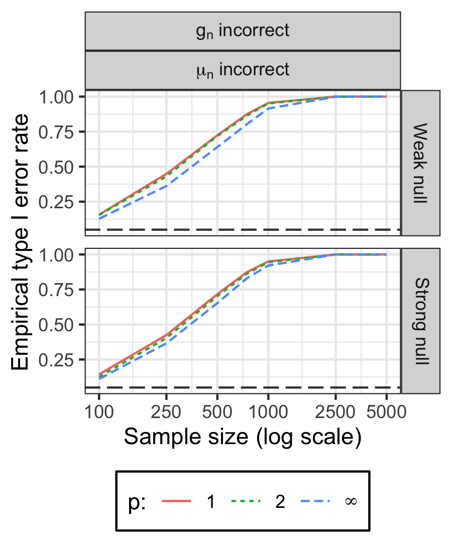
Figure 2: Empirical type I error rate of nominal α=0.05\alpha=0.05 level tests using the nonparametric nuisance estimators. The left column is our cross-fitted test with nonparametric nuisances estimators, the middle column is the same without cross-fitting, and the right column is a TMLE-based test using a dichotomized exposure. Horizontal wide-dash line indicates then nominal 0.05 test size, and horizontal dotted lines indicate expected sampling error bounds were the true size 0.05.

We now turn to the results of the simulation study. We focus on the results from the use of nonparametric nuisance estimators, since this is what we suggest to use in practice. The results from the use of parametric nuisance estimators were in line with expectations based on our theoretical results; full details of the results may be found in Supplementary Material. Figure 2 displays the empirical type I error rate for the three estimators with nonparametric nuisance estimators. Our tests with cross-fitted nuisance estimators (first column) had empirical error rates within Monte Carlo error of the nominal error rate at all sample sizes and under both the strong and weak nulls. This empirically validates the large-sample theoretical guarantee of Theorem 4, and also indicates that the type I error of the method is valid even for small sample sizes. However, the nonparametric nuisance estimators without cross-fitting (second column) had type I error significantly larger than 0.050.05 for n≤1000n\leq 1000. This suggests that the cross-fitting procedure reduced the bias of the estimator of Ω0\Omega_{0} and/or of the bias of the estimator of the quantile T0,α,pT_{0,\alpha,p} for small and moderate sample sizes, resulting in improved type I error rates. The TMLE-based test with a dichotomized exposure also had empirical error rates within Monte Carlo error of the nominal rate for all sample sizes under both types of null hypotheses, as expected.

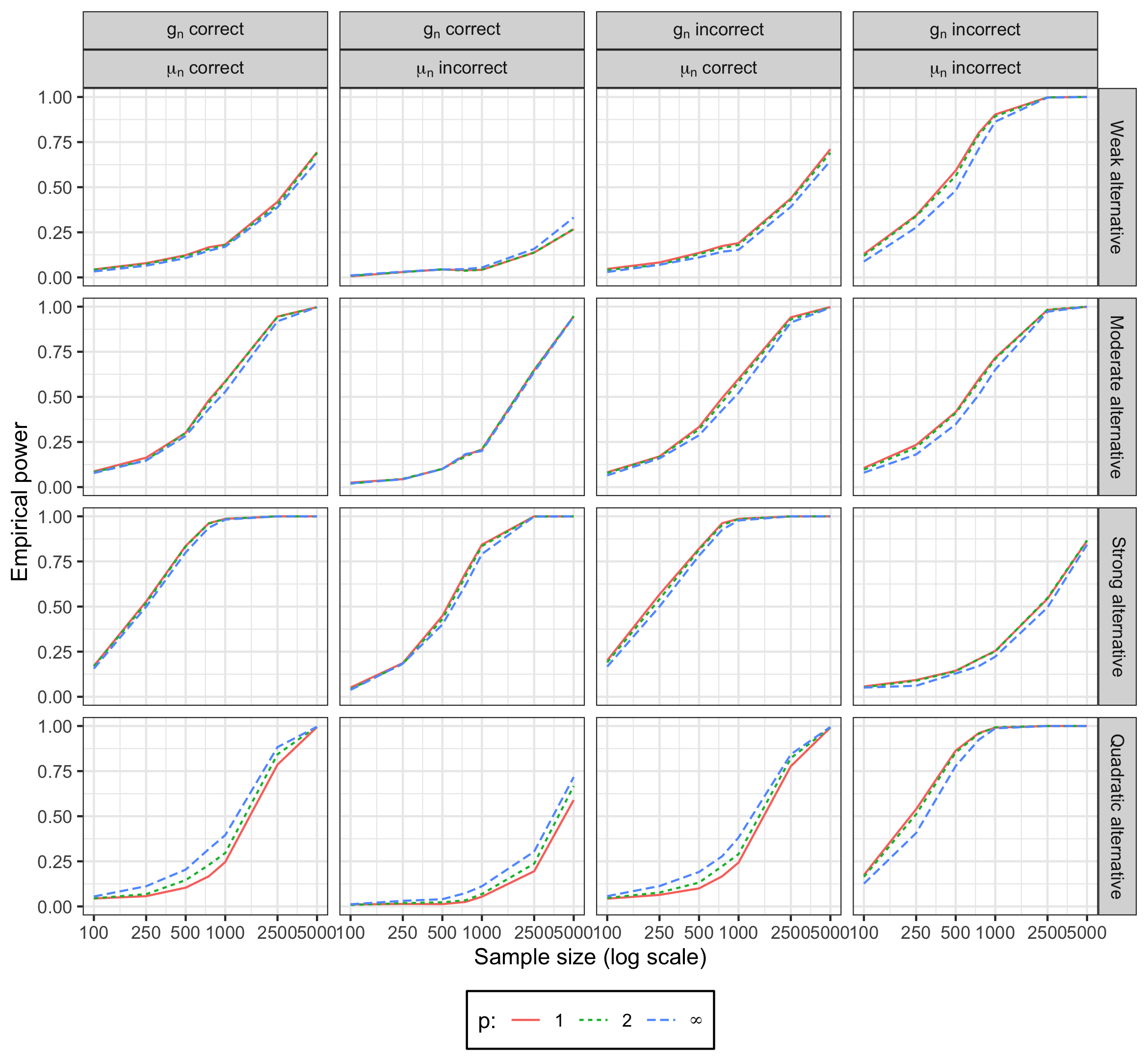
Figure 3 displays the empirical power using the nonparametric nuisance estimators. We omitted the estimator without cross-fitting, since this estimator had poor type I error control. Power was generally very low for n=100n=100, but increased with sample size and with distance from the null. For the three linear alternatives (first three rows), our test had only slightly (i.e. 5-10 percentage points) better power than the TMLE-based test using a dichotomized exposure. This makes sense, since the true effect size induced by dichotomization of the exposure increased with the slope of θ0\theta_{0} in the case that θ0\theta_{0} was linear. However, for the quadratic alternative, the test proposed here had substantially larger power than the TMLE-based test. For example, at sample size n=1000n=1000, the TMLE-based test had power 0.09, while our test had power between 0.25 and 0.35, and at sample size n=5000n=5000, the TMLE-based test had power 0.25, while our test had power near 0.85. This can be explained by the fact that the true effect size induced by dichotomization for the quadratic alternative was close to zero because the axis of symmetry for the parabolic effect curve was 0.5, the same as the point of dichotomization. This suggests that, as has been previously noted (e.g. Fedorov et al. 2009), dichotomization can result in substantial loss of power for certain types of data-generating mechanisms. Discretizing the exposure into more categories would increase the power of the TMLE-based test, but in practice it is hard to know what discretization will yield acceptable power without knowing the true form of θ0\theta_{0}.

Refer to caption
Figure 3: Empirical power of nominal α=0.05\alpha=0.05 level tests using nonparametric nuisance estimators. Columns indicate the alternative hypothesis used to generate the data, and rows indicate the method used to test the null hypothesis.

Overall, we observed little systematic difference in type I error rates between the three values of pp using either type of nuisance estimator for our test. For the linear alternatives, the test with p=∞p=\infty had consistently slightly smaller power than that with p=1p=1 or p=2p=2. However, for the quadratic alternative, the test with p=∞p=\infty had consistently larger power than the others. Therefore, which value of pp yields the greatest power depends on the shape of the true effect curve. As noted previously, we recommend using p=∞p=\infty in practice due in part to the improved power against nonlinear alternatives.

4.2 Simulation study II: discrete exposure with many levels

In a second simulation study, we assessed the effect of increasing the number of levels of a discrete exposure on the properties of tests of the null hypothesis of no average causal effect. We simulated three covariates W∈ℝ3W\in\mathbb{R}^{3} from independent uniform distributions on [−1,1][-1,1], [−1,1][-1,1], and [0,2][0,2], respectively. For a number of levels kk, we set P0​(A=a∣W=w)=logit−1​[(.5−a)​(βT​w)]/h⁡(w)P_{0}(A=a\mid W=w)=\mathrm{logit}^{-1}[(.5-a)(\beta^{T}w)]/h(w) for a∈{1/k,2/k,…,1}a\in\{1/k,2/k,\dotsc,1\}, and P0​(A=a∣W=w)=0P_{0}(A=a\mid W=w)=0 otherwise, where h⁡(w)h(w) is a normalizing constant. Given AA and WW, we simulated YY as in simulation study I described above. For each n∈{250,500,750}n\in\{250,500,750\}, we considered eight values of kk between k=5k=5 and k=n/2k=n/2, which allowed us to assess the effect of the number of discrete components of the exposure on the properties of testing procedures. For each setting, we simulated 1000 datasets, and used two methods to test the null hypothesis of no average causal effect of AA on YY. First, we used the method described here with p∈{1,2,∞}p\in\{1,2,\infty\}. Second, we used a chi-squared test based on an augmented IPW (AIPW) estimator of θ0​(aj)\theta_{0}(a_{j}) for each aja_{j} in the support of AA. Since the exposure was discrete, the AIPW-based test had asymptotically valid size for any fixed kk; our goal was to assess its finite-sample performance as a function of kk. For both tests, we used cross-fitted maximum likelihood estimators from correctly-specified parametric models for the nuisance estimators.

Refer to caption
Figure 4: Empirical type I error rate of nominal α=0.05\alpha=0.05 level tests in the second simulation study. The xx-axis is the ratio of kk, the number of levels of the exposure, to nn, the sample size. Columns indicate the null hypothesis used to generate the data, and rows indicate the method used to test the null hypothesis.

Figure 4 displays the empirical type I error of the two methods under the weak and strong null hypotheses. Our methods (bottom row) had type I error near 0.05 for all nn and kk considered. AIPW, on the other hand, only had valid type I error for the smallest value of kk considered (k=5k=5). As the number of levels of AA grew, the type I error rate of the AIPW-based test rapidly grew to 1. In Supplementary Material, we display the power of our test, which was constant in kk, and for all settings considered increased with nn. Therefore, use of the methods proposed here is not limited to exposures with a continuous component, but should be considered for all discrete exposures with more than a few values.

5 BMI and T-cell response in HIV vaccine studies

Numerous scientific studies have found a negative association between obesity or BMI and immune responses to vaccination. In Jin et al. 2015, the authors found that low BMI (<25<25) participants in early-phase HIV vaccine trials had a higher rate of CD4+ T cell response than high BMI (≥30\geq 30) participants. They also found a significant effect of BMI in a logistic regression of CD4+ responses on sex, age, BMI, vaccination dose, and number of vaccinations (OR: 0.92; 95% CI: 0.86–0.98; pp=0.007). However, as discussed in the introduction, this odds ratio only has a causal interpretation under strong parametric assumptions.

In Westling et al. 2020, the authors estimated the causal dose-response curve θ0\theta_{0}, adjusting for the same set of confounders as did Jin et al. 2015, under the assumption that it is decreasing. However, they did not assess the null hypothesis that the curve was flat. We note that Westling et al. 2020 estimated θ0​(20)−θ0​(35)\theta_{0}(20)-\theta_{0}(35), i.e. the difference between the probabilities of having a positive CD4+ immune response under assignment to BMIs of 20 and 35, to be 0.22, with 95% confidence interval 0.03–0.41. However, this confidence interval is only valid under the assumption that θ0​(20)>θ0​(35)\theta_{0}(20)>\theta_{0}(35), and hence cannot be used as evidence against the null hypothesis that θ0\theta_{0} is flat. Furthermore, the fact that the lower end of this confidence interval is relatively close to zero suggests that there may not actually be strong evidence against this null. Here, we formally assess this null hypothesis using the same data as Westling et al. 2020.

The data consist of pooled vaccine arms from 11 phase I/II clinical trials conducted through the HIV Vaccine Trials Network (HVTN). Descriptions of these trials may be found in Jin et al. 2015 and Westling et al. 2020. CD4+ and CD8+ T-cell responses at the first visit following administration of the last vaccine dose were measured using validated intracellular cytokine staining, and these continuous responses were converted to binary indicators of whether there was a significant change from baseline using the method described in Jin et al. 2015. After excluding three participants with missing BMI and participants with missing immune response, our analysis datasets consisted of a total of n=439n=439 participants for the analysis of CD4+ responses and n=462n=462 participants for CD8+ responses.

We tested the null hypotheses that there is a causal effect of BMI on CD4+ and CD8+ T-cell responses using the method developed in this paper with p=∞p=\infty and V=10V=10 folds. To estimate the outcome regression μ0\mu_{0} and the propensity score g0g_{0}, we used SuperLearner (van der Laan et al. 2007; Díaz and van der Laan 2011) with flexible libraries consisting of generalized linear models, generalized additive models, multivariate regression splines, random forests, and gradient boosting. For the analysis of the effect of BMI on CD4+ responses, we found p=0.16p=0.16, and for the analysis of the effect of BMI on CD8+ responses, we found p=0.22p=0.22. Hence, we do not find evidence of a causal effect of BMI on the probability of having a positive immune response in these data. Plots of Ωn\Omega_{n} are presented in Supplementary Material.

6 Discussion

We have presented a nonparametric method for testing the null hypothesis that a causal dose-response curve is flat, for use in observational studies with no unobserved confounding. The key idea behind our test was to translate the null hypothesis on the parameter of interest, which is not a pathwise differentiable parameter in the nonparametric model, into a null hypothesis on a primitive parameter, which is pathwise differentiable.

In addition to permitting the use of methods and theory for pathwise differentiable parameters, using the primitive function gives our tests non-trivial power to detect alternatives approaching the null at the rate n−1/2n^{-1/2}. However, results from the literature concerning tests of marginal regression functions suggest that any test able to detect n−1/2n^{-1/2}-rate alternatives must necessarily have low finite-sample power against certain smooth alternatives (Horowitz and Spokoiny 2001). Analogous results regarding causal dose-response functions are not to our knowledge available, but we conjecture that appropriate parallels can be established. Therefore, our tests may have poor finite-sample power against certain shapes of dose-response functions; in particular, functions that are nearly flat except for a sharp peak in a narrow range of the support of the exposure. We suggest that users conduct numerical studies on the power of our tests if they expect that their dose-response function may look like this. Tests based on an estimator of the dose-response function, which to our knowledge do not yet exist, may not have this problem, although such tests would also have slower than n−1/2n^{-1/2} rates of convergence. We leave further inquiry along these lines to future work.

An additional benefit of using the primitive function defined here is that it makes the test agnostic to the marginal distribution of the exposure: the test works equally well with discrete, continuous, and mixed discrete-continuous exposures. This was validated in numerical studies, where in particular we demonstrated that a traditional doubly-robust test of no average causal effect in the setting of a fully discrete exposure quickly became invalid as the number of levels of the exposure grew. We note that tests based on directly estimating the dose-response function, such as tests based on the local linear estimator, may only work in the context of fully continuous exposures.

Several modifications of the proposed test may be of interest in future research. Here, we studied the properties of the test for fixed values of pp. In numerical studies, we found little difference in the performance of the test for p∈{1,2,∞}p\in\{1,2,\infty\}, and we do not expect that the choice of pp would drastically change the results in most cases. However, the results presented herein were for fixed values of pp, and so if a researcher were to select a value of pp based on the results of the test, the test may no longer have asymptotically valid type I error. In future research, it would be of interest to adaptively select a value of pp to maximize power while retaining type I error control. In addition, here, we used the empirical distribution function as our weight function to assess whether the primitive parameter is flat. Alternative weight functions could be used to, for instance, place more emphasis in the tails or center of the distribution of the exposure, or a weight function could possibly be adaptively chosen to maximize power. Finally, while we used a one-step estimator of the primitive parameter, TMLE could be used instead.

Supplementary Material for:

Nonparametric tests of the causal null
with non-discrete exposures

Proof of Theorems

Proof of Proposition 1.

(1)⟹\implies(2): Let a∈𝒜0a\in\mathscr{A}_{0}. Then, since θ0​(u)=θ0​(a)\theta_{0}(u)=\theta_{0}(a) for all u∈𝒜0u\in\mathscr{A}_{0}, γ0=∫θ0​(u)​d​F0​(u)=∫θ0​(a)​d​F0​(u)=θ0​(a)\gamma_{0}=\int\theta_{0}(u)\,dF_{0}(u)=\int\theta_{0}(a)\,dF_{0}(u)=\theta_{0}(a).

(2)⟹\implies(1): trivial.

(2)⟹\implies(3): Let a∈ℝa\in\mathbb{R}. Then Γ0​(a)=∫−∞aθ0​(u)​d​F0​(u)=γ0​F0​(a)\Gamma_{0}(a)=\int_{-\infty}^{a}\theta_{0}(u)\,dF_{0}(u)=\gamma_{0}F_{0}(a), so Ω0​(a)=0\Omega_{0}(a)=0.

(3)⟹\implies(2): We proceed by contradiction: suppose that θ0​(a)≠γ0\theta_{0}(a)\neq\gamma_{0} for some a∈𝒜0a\in\mathscr{A}_{0}. We assume first that θ0​(a)−γ0=δ>0\theta_{0}(a)-\gamma_{0}=\delta>0. Then since by assumption θ0\theta_{0} is continuous on 𝒜0\mathscr{A}_{0}, there exists ε>0\varepsilon>0 such that |θ0​(u)−θ0​(a)|≤δ/2|\theta_{0}(u)-\theta_{0}(a)|\leq\delta/2 for all u∈𝒜0∩[a−ε,a+ε]u\in\mathscr{A}_{0}\cap[a-\varepsilon,a+\varepsilon], which implies that θ0​(u)−γ0≥δ/2\theta_{0}(u)-\gamma_{0}\geq\delta/2 for all such uu. We then have

0=Ω0​(a+ε)−Ω0​(a−ε)\displaystyle 0=\Omega_{0}(a+\varepsilon)-\Omega_{0}(a-\varepsilon) =∫a−εa+ε[θ0(u)−γ0]dF0(u)=∫(a−ε,a+ε]∩𝒜0[θ0(u)−γ0]dF0(u)\displaystyle=\int_{a-\varepsilon}^{a+\varepsilon}[\theta_{0}(u)-\gamma_{0}]\,dF_{0}(u)=\int_{(a-\varepsilon,a+\varepsilon]\cap\mathscr{A}_{0}}[\theta_{0}(u)-\gamma_{0}]\,dF_{0}(u)
≥(δ/2)​[F0​(a+ε)−F0​(a−ε)]>0,\displaystyle\geq(\delta/2)\left[F_{0}(a+\varepsilon)-F_{0}(a-\varepsilon)\right]>0\ ,

where the last inequality follows because aa is in the support of F0F_{0}. This is a contradiction, and therefore θ0​(a)≤γ0\theta_{0}(a)\leq\gamma_{0}. The argument if θ0​(a)<γ0\theta_{0}(a)<\gamma_{0} is essentially identical, and since a∈𝒜0a\in\mathscr{A}_{0} was arbitrary, this yields that θ0​(a)=γ0\theta_{0}(a)=\gamma_{0} for all a∈𝒜0a\in\mathscr{A}_{0}.

(3)⟹\implies(4): trivial.

(4)⟹\implies(3): We proceed again by contradiction. Suppose |Ω0​(a)|>0|\Omega_{0}(a)|>0 for some a∈ℝa\in\mathbb{R}. First suppose a∈𝒜0a\in\mathscr{A}_{0}. If aa is a mass point of F0F_{0}, then clearly ‖Ω0‖F0,1>0\|\Omega_{0}\|_{F_{0},1}>0, a contradiction. If aa is not a mass point of F0F_{0}, then for any ε>0\varepsilon>0

|Ω0​(a+ε)−Ω0​(a)|≤∫aa+ε|θ0​(u)−γ0|​d​F0​(u)≤c⁡[F0​(a+ε)−F0​(a)]\left|\Omega_{0}(a+\varepsilon)-\Omega_{0}(a)\right|\leq\int_{a}^{a+\varepsilon}\left|\theta_{0}(u)-\gamma_{0}\right|\,dF_{0}(u)\leq c[F_{0}(a+\varepsilon)-F_{0}(a)]

for c<∞c<\infty, and since F0​(a+ε)→F0​(a)F_{0}(a+\varepsilon)\to F_{0}(a) as ε→0\varepsilon\to 0, Ω0\Omega_{0} is right-continuous at aa. An analogous argument shows that Ω0\Omega_{0} is also left-continuous at aa. This implies that |Ω0||\Omega_{0}| is positive in a neighborhood of aa, which implies since a∈𝒜0a\in\mathscr{A}_{0} that ‖Ω0‖F0,1>0\|\Omega_{0}\|_{F_{0},1}>0, a contradiction. Finally, if a∈ℝa\in\mathbb{R} is not an element of 𝒜0\mathscr{A}_{0}, then Ω0​(a)=Ω0​(a0)\Omega_{0}(a)=\Omega_{0}(a_{0}) for a0:=sup{u∈𝒜0:u<a}a_{0}:=\sup\{u\in\mathscr{A}_{0}:u<a\}, so that |Ω0​(a)|>0|\Omega_{0}(a)|>0 implies |Ω0​(a0)|>0|\Omega_{0}(a_{0})|>0, and since a0∈𝒜0a_{0}\in\mathscr{A}_{0} (because 𝒜0\mathscr{A}_{0} is closed), this leads to a contradiction.

∎

Proof of Proposition 2.

We let {Pε:|ε|≤δ}\left\{P_{\varepsilon}:|\varepsilon|\leq\delta\right\} be any one-dimensional differentiable in quadratic mean (DQM) path in ℳ∘\mathscr{M}^{\circ} such that Pε=0=P0P_{\varepsilon=0}=P_{0}, where ℳ∘\mathscr{M}^{\circ} be the subset of P∈ℳP\in\mathscr{M} such that there exists η>0\eta>0 such that gP​(a,w)≥ηg_{P}(a,w)\geq\eta for PP-a.e. (a,w)}(a,w)\} and EP​[Y2]<∞E_{P}[Y^{2}]<\infty. We let (y,a,w)↦ℓ˙0​(y,a,w)(y,a,w)\mapsto\dot{\ell}_{0}(y,a,w) be the score function of the path at ε=0\varepsilon=0, We note that P0​ℓ˙0=0P_{0}\dot{\ell}_{0}=0 and P0​ℓ˙02<∞P_{0}\dot{\ell}_{0}^{2}<\infty (Bickel et al. 1998). Furthermore, we define ℓ˙0(a,w):=E0[ℓ˙0∣A=a,W=w]\dot{\ell}_{0}(a,w):=E_{0}[\dot{\ell}_{0}\mid A=a,W=w] and analogously ℓ˙0​(a)\dot{\ell}_{0}(a) and ℓ˙0​(w)\dot{\ell}_{0}(w) as the marginal score functions and ℓ˙0​(y∣a,w):=ℓ˙0​(y,a,w)−ℓ˙0​(a,w)\dot{\ell}_{0}(y\mid a,w):=\dot{\ell}_{0}(y,a,w)-\dot{\ell}_{0}(a,w) as the conditional score function, which has mean zero conditional given A,WA,W under P0P_{0}.

The nonparametric efficient influence function Da0,0∗D_{a_{0},0}^{*} of Ω0​(a0)\Omega_{0}(a_{0}) can be derived by showing that ∂∂ε​Ωε​(a0)|ε=0=P0​(Da0,0∗​ℓ˙0)\left.\frac{\partial}{\partial\varepsilon}\Omega_{\varepsilon}(a_{0})\right|_{\varepsilon=0}=P_{0}\left(D_{a_{0},0}^{*}\dot{\ell}_{0}\right). We have by definition of Ω0\Omega_{0} and ordinary rules of calculus that

∂∂ε​Ωε​(a0)|ε=0\displaystyle\left.\frac{\partial}{\partial\varepsilon}\Omega_{\varepsilon}(a_{0})\right|_{\varepsilon=0} =∂∂ε​Γε​(a0)|ε=0−∂∂ε​γε|ε=0​F0​(a0)−γ0​∂∂ε​Fε​(a0)|ε=0.\displaystyle=\left.\frac{\partial}{\partial\varepsilon}\Gamma_{\varepsilon}(a_{0})\right|_{\varepsilon=0}-\left.\frac{\partial}{\partial\varepsilon}\gamma_{\varepsilon}\right|_{\varepsilon=0}F_{0}(a_{0})-\gamma_{0}\left.\frac{\partial}{\partial\varepsilon}F_{\varepsilon}(a_{0})\right|_{\varepsilon=0}. (5)

We first note that since FP​(a0)=EP​[I⁡(A≤a0)]=∫I⁡(a≤a0)​𝑑P​(Y,A,W)F_{P}(a_{0})=E_{P}[I(A\leq a_{0})]=\int I(a\leq a_{0})\,dP(Y,A,W) for any PP,

∂∂ε​Fε​(a0)|ε=0\displaystyle\left.\frac{\partial}{\partial\varepsilon}F_{\varepsilon}(a_{0})\right|_{\varepsilon=0} =∂∂ε​∫I⁡(a≤a0)​d​Pε​(y,a,w)|ε=0=∫I⁡(a≤a0)​ℓ˙0​(y,a,w)​d​P0​(y,a,w)\displaystyle=\left.\frac{\partial}{\partial\varepsilon}\int I(a\leq a_{0})dP_{\varepsilon}(y,a,w)\right|_{\varepsilon=0}=\int I(a\leq a_{0})\dot{\ell}_{0}(y,a,w)dP_{0}(y,a,w)
=E0​[I⁡(A≤a0)​ℓ˙0​(Y,A,W)].\displaystyle=E_{0}\left[I(A\leq a_{0})\dot{\ell}_{0}(Y,A,W)\right].

Therefore, the term γ0​∂∂ε​Fε​(a0)|ε=0\gamma_{0}\left.\frac{\partial}{\partial\varepsilon}F_{\varepsilon}(a_{0})\right|_{\varepsilon=0} in (5) contributes −γ0​I​(a≤a0)-\gamma_{0}I(a\leq a_{0}) to the uncentered influence function.

Next, by definitions of ΓP\Gamma_{P} and γP\gamma_{P} and the product rule,

∂∂ε​Γε​(a0)|ε=0−∂∂ε​γε|ε=0​F0​(a0)\displaystyle\left.\frac{\partial}{\partial\varepsilon}\Gamma_{\varepsilon}(a_{0})\right|_{\varepsilon=0}-\left.\frac{\partial}{\partial\varepsilon}\gamma_{\varepsilon}\right|_{\varepsilon=0}F_{0}(a_{0}) =∂∂ε​∬I⁡(a≤a0)​με​(a,w)​d​Fε​(a)​d​Qε​(w)|ε=0\displaystyle=\left.\frac{\partial}{\partial\varepsilon}\iint I(a\leq a_{0})\mu_{\varepsilon}(a,w)\,dF_{\varepsilon}(a)\,dQ_{\varepsilon}(w)\right|_{\varepsilon=0}
−∂∂ε∬με(a,w)dFε(a)dQε(w)|ε=0F0(a0)\displaystyle\qquad-\left.\frac{\partial}{\partial\varepsilon}\iint\mu_{\varepsilon}(a,w)\,dF_{\varepsilon}(a)\,dQ_{\varepsilon}(w)\right|_{\varepsilon=0}F_{0}(a_{0})
=∂∂ε​∬[I⁡(a≤a0)−F0​(a0)]​με​(a,w)​d​Fε​(a)​d​Qε​(w)|ε=0\displaystyle=\left.\frac{\partial}{\partial\varepsilon}\iint\left[I(a\leq a_{0})-F_{0}(a_{0})\right]\mu_{\varepsilon}(a,w)\,dF_{\varepsilon}(a)\,dQ_{\varepsilon}(w)\right|_{\varepsilon=0}
=∂∂ε​∭[I⁡(a≤a0)−F0​(a0)]​y​d​Pε​(y∣a,w)​d​F0​(a)​d​Q0​(w)|ε=0\displaystyle=\left.\frac{\partial}{\partial\varepsilon}\iiint\left[I(a\leq a_{0})-F_{0}(a_{0})\right]y\,dP_{\varepsilon}(y\mid a,w)\,dF_{0}(a)\,dQ_{0}(w)\right|_{\varepsilon=0}
+∂∂ε∬[I(a≤a0)−F0(a0)]μ0(a,w)dFε(a)dQ0(w)|ε=0\displaystyle\qquad+\left.\frac{\partial}{\partial\varepsilon}\iint\left[I(a\leq a_{0})-F_{0}(a_{0})\right]\mu_{0}(a,w)\,dF_{\varepsilon}(a)\,dQ_{0}(w)\right|_{\varepsilon=0}
+∂∂ε∬[I(a≤a0)−F0(a0)]μ0(a,w)dF0(a)dQε(w)|ε=0.\displaystyle\qquad+\left.\frac{\partial}{\partial\varepsilon}\iint\left[I(a\leq a_{0})-F_{0}(a_{0})\right]\mu_{0}(a,w)\,dF_{0}(a)\,dQ_{\varepsilon}(w)\right|_{\varepsilon=0}.

Now using basic properties of score functions, we have

∂∂ε​∭[I⁡(a≤a0)−F0​(a0)]​y​d​Pε​(y∣a,w)​d​F0​(a)​d​Q0​(w)|ε=0\displaystyle\left.\frac{\partial}{\partial\varepsilon}\iiint\left[I(a\leq a_{0})-F_{0}(a_{0})\right]y\,dP_{\varepsilon}(y\mid a,w)\,dF_{0}(a)\,dQ_{0}(w)\right|_{\varepsilon=0}
=∭[I⁡(a≤a0)−F0​(a0)]​y​ℓ˙0​(y∣a,w)​d​P0​(y∣a,w)​d​F0​(a)​d​Q0​(w)\displaystyle\qquad=\iiint\left[I(a\leq a_{0})-F_{0}(a_{0})\right]y\dot{\ell}_{0}(y\mid a,w)\,dP_{0}(y\mid a,w)\,dF_{0}(a)\,dQ_{0}(w)
=E0​{[I⁡(A≤a0)−F0​(a0)]​Yg0​(A,W)​ℓ˙0​(Y∣A,W)}\displaystyle\qquad=E_{0}\left\{\left[I(A\leq a_{0})-F_{0}(a_{0})\right]\frac{Y}{g_{0}(A,W)}\dot{\ell}_{0}(Y\mid A,W)\right\}
=E0​{[I⁡(A≤a0)−F0​(a0)]​Yg0​(A,W)​[ℓ˙0​(Y,A,W)−ℓ˙0​(A,W)]}\displaystyle\qquad=E_{0}\left\{\left[I(A\leq a_{0})-F_{0}(a_{0})\right]\frac{Y}{g_{0}(A,W)}\left[\dot{\ell}_{0}(Y,A,W)-\dot{\ell}_{0}(A,W)\right]\right\}
=E0​{[I⁡(A≤a0)−F0​(a0)]​Yg0​(A,W)​ℓ˙0​(Y,A,W)}\displaystyle\qquad=E_{0}\left\{\left[I(A\leq a_{0})-F_{0}(a_{0})\right]\frac{Y}{g_{0}(A,W)}\dot{\ell}_{0}(Y,A,W)\right\}
−E0​{[I⁡(A≤a0)−F0​(a0)]​E0[Y∣A,W]g0​(A,W)​ℓ˙0​(A,W)}\displaystyle\qquad\qquad-E_{0}\left\{\left[I(A\leq a_{0})-F_{0}(a_{0})\right]\frac{E_{0}\left[Y\mid A,W\right]}{g_{0}(A,W)}\dot{\ell}_{0}(A,W)\right\}
=E0​{[I⁡(A≤a0)−F0​(a0)]​Yg0​(A,W)​ℓ˙0​(Y,A,W)}\displaystyle\qquad=E_{0}\left\{\left[I(A\leq a_{0})-F_{0}(a_{0})\right]\frac{Y}{g_{0}(A,W)}\dot{\ell}_{0}(Y,A,W)\right\}
−E0​{[I⁡(A≤a0)−F0​(a0)]​μ0​(A,W)g0​(A,W)​ℓ˙0​(Y,A,W)}\displaystyle\qquad\qquad-E_{0}\left\{\left[I(A\leq a_{0})-F_{0}(a_{0})\right]\frac{\mu_{0}(A,W)}{g_{0}(A,W)}\dot{\ell}_{0}(Y,A,W)\right\}
=E0​{[I⁡(A≤a0)−F0​(a0)]​Y−μ0​(A,W)g0​(A,W)​ℓ˙0​(Y,A,W)}\displaystyle\qquad=E_{0}\left\{\left[I(A\leq a_{0})-F_{0}(a_{0})\right]\frac{Y-\mu_{0}(A,W)}{g_{0}(A,W)}\dot{\ell}_{0}(Y,A,W)\right\}

since E0​[h⁡(A,W)​ℓ˙0​(A,W)]=E0​[h⁡(A,W)​ℓ˙0​(Y,A,W)]E_{0}[h(A,W)\dot{\ell}_{0}(A,W)]=E_{0}[h(A,W)\dot{\ell}_{0}(Y,A,W)] for any suitable hh. Note that we have used the assumption that g0g_{0} is almost surely positive in the above derivation. We also have

∂∂ε​∬[I⁡(a≤a0)−F0​(a0)]​μ0​(a,w)​d​Fε​(a)​d​Q0​(w)|ε=0\displaystyle\left.\frac{\partial}{\partial\varepsilon}\iint\left[I(a\leq a_{0})-F_{0}(a_{0})\right]\mu_{0}(a,w)\,dF_{\varepsilon}(a)\,dQ_{0}(w)\right|_{\varepsilon=0}
=∬[I⁡(a≤a0)−F0​(a0)]​μ0​(a,w)​ℓ˙0​(a)​d​F0​(a)​d​Q0​(w)\displaystyle\qquad=\iint\left[I(a\leq a_{0})-F_{0}(a_{0})\right]\mu_{0}(a,w)\dot{\ell}_{0}(a)\,dF_{0}(a)\,dQ_{0}(w)
=∫[I⁡(a≤a0)−F0​(a0)]​θ0​(a)​ℓ˙0​(a)​d​F0​(a)\displaystyle\qquad=\int\left[I(a\leq a_{0})-F_{0}(a_{0})\right]\theta_{0}(a)\dot{\ell}_{0}(a)\,dF_{0}(a)
=E0​{[I⁡(A≤a0)−F0​(a0)]​θ0​(A)​ℓ˙0​(A)}\displaystyle\qquad=E_{0}\left\{\left[I(A\leq a_{0})-F_{0}(a_{0})\right]\theta_{0}(A)\dot{\ell}_{0}(A)\right\}
=E0​{[I⁡(A≤a0)−F0​(a0)]​θ0​(A)​ℓ˙0​(Y,A,W)}\displaystyle\qquad=E_{0}\left\{\left[I(A\leq a_{0})-F_{0}(a_{0})\right]\theta_{0}(A)\dot{\ell}_{0}(Y,A,W)\right\}

by an analogous argument, and similarly

∂∂ε​∬[I⁡(a≤a0)−F0​(a0)]​μ0​(a,w)​d​F0​(a)​d​Qε​(w)|ε=0\displaystyle\left.\frac{\partial}{\partial\varepsilon}\iint\left[I(a\leq a_{0})-F_{0}(a_{0})\right]\mu_{0}(a,w)\,dF_{0}(a)\,dQ_{\varepsilon}(w)\right|_{\varepsilon=0}
=∬[I⁡(a≤a0)−F0​(a0)]​μ0​(a,w)​ℓ˙0​(w)​d​F0​(a)​d​Q0​(w)\displaystyle\qquad=\iint\left[I(a\leq a_{0})-F_{0}(a_{0})\right]\mu_{0}(a,w)\dot{\ell}_{0}(w)\,dF_{0}(a)\,dQ_{0}(w)
=E0​{∫[I⁡(a≤a0)−F0​(a0)]​μ0​(a,W)​d​F0​(a)​ℓ˙0​(W)}\displaystyle\qquad=E_{0}\left\{\int\left[I(a\leq a_{0})-F_{0}(a_{0})\right]\mu_{0}(a,W)\,dF_{0}(a)\dot{\ell}_{0}(W)\right\}
=E0​{∫[I⁡(a≤a0)−F0​(a0)]​μ0​(a,W)​d​F0​(a)​ℓ˙0​(Y,A,W)}.\displaystyle\qquad=E_{0}\left\{\int\left[I(a\leq a_{0})-F_{0}(a_{0})\right]\mu_{0}(a,W)\,dF_{0}(a)\dot{\ell}_{0}(Y,A,W)\right\}.

Putting it together, the uncentered influence function is

[I⁡(a≤a0)−F0​(a0)]​[y−μ0​(a,w)g0​(a,w)+θ0​(a)]+∫[I⁡(u≤a0)−F0​(a0)]​μ0​(u,w)​d​F0​(u)−γ0​I​(a≤a0).\displaystyle\left[I(a\leq a_{0})-F_{0}(a_{0})\right]\left[\frac{y-\mu_{0}(a,w)}{g_{0}(a,w)}+\theta_{0}(a)\right]+\int\left[I(u\leq a_{0})-F_{0}(a_{0})\right]\mu_{0}(u,w)\,dF_{0}(u)-\gamma_{0}I(a\leq a_{0}).

Influence functions have mean zero, so we need to subtract the mean under P0P_{0} of this uncentered function to obtain the centered influence function. The mean under P0P_{0} of this function is 2​Ω0​(a0)+γ0​F0​(a0)2\Omega_{0}(a_{0})+\gamma_{0}F_{0}(a_{0}), so the centered influence function is

[I⁡(a≤a0)−F0​(a0)]​[y−μ0​(a,w)g0​(a,w)+θ0​(a)−γ0]\displaystyle\left[I(a\leq a_{0})-F_{0}(a_{0})\right]\left[\frac{y-\mu_{0}(a,w)}{g_{0}(a,w)}+\theta_{0}(a)-\gamma_{0}\right]
+∫[I(u≤a0)−F0(a0)]μ0(u,w)dF0(u)−2Ω0(a0),\displaystyle\qquad+\int\left[I(u\leq a_{0})-F_{0}(a_{0})\right]\mu_{0}(u,w)\,dF_{0}(u)-2\Omega_{0}(a_{0}),

which equals Da0,0∗​(y,a,w)D_{a_{0},0}^{*}(y,a,w) as claimed. When g0g_{0} is almost surely bounded away from zero and E0​[Y2]<∞E_{0}[Y^{2}]<\infty, this function has finite variance. ∎

Before proving our main results, we derive a first-order expansion of Ωn∘​(a)\Omega_{n}^{\circ}(a). We define

Da0,n,v​(y,a,w)\displaystyle D_{a_{0},n,v}(y,a,w) :=[I(−∞,a0](a)−Fn,v(a0)][y−μn,v​(a,w)gn,v​(a,w)+θμn,v,Qn,v(a)−γμn,v,Fn,v,Qn,v]\displaystyle:=\left[I_{(-\infty,a_{0}]}(a)-F_{n,v}(a_{0})\right]\left[\frac{y-\mu_{n,v}(a,w)}{g_{n,v}(a,w)}+\theta_{\mu_{n,v},Q_{n,v}}(a)-\gamma_{\mu_{n,v},F_{n,v},Q_{n,v}}\right]
+∫[I(−∞,a0](a~)−F0(a0)]μn,v(a~,w)F0(da~)−Ωμn,v,F0,Qn,v(a0),\displaystyle\qquad+\int\left[I_{(-\infty,a_{0}]}(\tilde{a})-F_{0}(a_{0})\right]\mu_{n,v}(\tilde{a},w)F_{0}(d\tilde{a})-\Omega_{\mu_{n,v},F_{0},Q_{n,v}}(a_{0})\ ,
Da0,μ,g​(y,a,w)\displaystyle D_{a_{0},\mu,g}(y,a,w) :=[I(−∞,a0](a)−F0(a0)][y−μ⁡(a,w)g⁡(a,w)+θμ,Q0(a)−γμ,F0,Q0]\displaystyle:=\left[I_{(-\infty,a_{0}]}(a)-F_{0}(a_{0})\right]\left[\frac{y-\mu(a,w)}{g(a,w)}+\theta_{\mu,Q_{0}}(a)-\gamma_{\mu,F_{0},Q_{0}}\right]
+∫[I(−∞,a0](a~)−F0(a0)]μ(a~,w)F0(da~)−Ωμ,F0,Q0(a0)\displaystyle\qquad+\int\left[I_{(-\infty,a_{0}]}(\tilde{a})-F_{0}(a_{0})\right]\mu(\tilde{a},w)F_{0}(d\tilde{a})-\Omega_{\mu,F_{0},Q_{0}}(a_{0})
Da0,n,v∘​(y,a,w)\displaystyle D_{a_{0},n,v}^{\circ}(y,a,w) :=[I(−∞,a0](a)−Fn,v(a0)][y−μn,v​(a,w)gn,v​(a,w)+θμn,v,Q0(a)]\displaystyle:=\left[I_{(-\infty,a_{0}]}(a)-F_{n,v}(a_{0})\right]\left[\frac{y-\mu_{n,v}(a,w)}{g_{n,v}(a,w)}+\theta_{\mu_{n,v},Q_{0}}(a)\right]
+∫[I(−∞,a0](a~)−F0(a0)]μn,v(a~,w)F0(da~)\displaystyle\qquad+\int\left[I_{(-\infty,a_{0}]}(\tilde{a})-F_{0}(a_{0})\right]\mu_{n,v}(\tilde{a},w)F_{0}(d\tilde{a})
Da0,∞∘​(y,a,w)\displaystyle D_{a_{0},\infty}^{\circ}(y,a,w) :=[I(−∞,a0](a)−F0(a0)][y−μ∞​(a,w)g∞​(a,w)+θμ∞,Q0(a)]\displaystyle:=\left[I_{(-\infty,a_{0}]}(a)-F_{0}(a_{0})\right]\left[\frac{y-\mu_{\infty}(a,w)}{g_{\infty}(a,w)}+\theta_{\mu_{\infty},Q_{0}}(a)\right]
+∫[I(−∞,a0](a~)−F0(a0)]μ∞(a~,w)F0(da~)\displaystyle\qquad+\int\left[I_{(-\infty,a_{0}]}(\tilde{a})-F_{0}(a_{0})\right]\mu_{\infty}(\tilde{a},w)F_{0}(d\tilde{a})
Da0,∞\displaystyle D_{a_{0},\infty} :=Da0,μ∞,g∞\displaystyle:=D_{a_{0},\mu_{\infty},g_{\infty}}
Da0,∞∗\displaystyle D_{a_{0},\infty}^{*} :=Da0,∞−Ω0​(a0)\displaystyle:=D_{a_{0},\infty}-\Omega_{0}(a_{0})

and

Rn,a0,v,1\displaystyle R_{n,a_{0},v,1} :=(ℙn,v−P0)​(Da0,n,v∘−Da0,∞∘),\displaystyle:=(\mathbb{P}_{n,v}-P_{0})\left(D_{a_{0},n,v}^{\circ}-D_{a_{0},\infty}^{\circ}\right)\ ,
Rn,a0,v,2\displaystyle R_{n,a_{0},v,2} :=(γμn,v,F0,Q0−γμn,v,F0,Qn,v−γμ0,F0,Q0+γμ∞,F0,Q0)​[Fn,v​(a0)−F0​(a0)]\displaystyle:=\left(\gamma_{\mu_{n,v},F_{0},Q_{0}}-\gamma_{\mu_{n,v},F_{0},Q_{n,v}}-\gamma_{\mu_{0},F_{0},Q_{0}}+\gamma_{\mu_{\infty},F_{0},Q_{0}}\right)\left[F_{n,v}(a_{0})-F_{0}(a_{0})\right]
Rn,a0,v,3\displaystyle R_{n,a_{0},v,3} :=∬[I(−∞,a0](a)−Fn,v(a0)]μn,v(a,w)(Fn,v−F0)(da)(Qn,v−Q0)(dw)\displaystyle:=\iint\left[I_{(-\infty,a_{0}]}(a)-F_{n,v}(a_{0})\right]\mu_{n,v}(a,w)\,(F_{n,v}-F_{0})(da)\,(Q_{n,v}-Q_{0})(dw)
Rn,a0,v,4\displaystyle R_{n,a_{0},v,4} :=∬[I(−∞,a0](a)−Fn,v(a0)][μn,v(a,w)−μ0(a,w)][1−g0​(a,w)gn,v​(a,w)]F0(da)Q0(dw)\displaystyle:=\iint\left[I_{(-\infty,a_{0}]}(a)-F_{n,v}(a_{0})\right]\left[\mu_{n,v}(a,w)-\mu_{0}(a,w)\right]\left[1-\frac{g_{0}(a,w)}{g_{n,v}(a,w)}\right]\,F_{0}(da)\,Q_{0}(dw)
Rn,a0,v,5\displaystyle R_{n,a_{0},v,5} :=(1−V​Nvn)​ℙn,v​Da0,∞∗.\displaystyle:=\left(1-\frac{VN_{v}}{n}\right)\mathbb{P}_{n,v}D_{a_{0},\infty}^{*}\ .
Lemma 1 (First-order expansion of estimator).

If condition (A3) or (A4) holds, then Ωn∘​(a0)−Ω0​(a0)=ℙn​Da0,∞∗+1V​∑v=1V∑j=15Rn,a0,v,j.\Omega_{n}^{\circ}(a_{0})-\Omega_{0}(a_{0})=\mathbb{P}_{n}D_{a_{0},\infty}^{*}+\frac{1}{V}\sum_{v=1}^{V}\sum_{j=1}^{5}R_{n,a_{0},v,j}.

Proof of Lemma 1.

We recall that θμ,Q​(a):=∫μ⁡(a,w)​Q​(𝑑w)\theta_{\mu,Q}(a):=\int\mu(a,w)\,Q(dw),

Ωμ,F,Q(a):=∬[I(−∞,a0](a)−F(a0)]μ(a,w)F(da)Q(dw),\Omega_{\mu,F,Q}(a):=\iint\left[I_{(-\infty,a_{0}]}(a)-F(a_{0})\right]\mu(a,w)\,F(da)\,Q(dw)\ ,

and γμ,F,Q:=∬μ⁡(a,w)​F​(𝑑a)​Q​(𝑑w)\gamma_{\mu,F,Q}:=\iint\mu(a,w)\,F(da)\,Q(dw). We thus have Ωn∘​(a0)=1V​∑v=1Vℙn,v​Da0,n,v\Omega_{n}^{\circ}(a_{0})=\frac{1}{V}\sum_{v=1}^{V}\mathbb{P}_{n,v}D_{a_{0},n,v}. If (A3) or (A4) hold, then

P0​Da0,∞\displaystyle P_{0}D_{a_{0},\infty} =Ω0(a0)+∬[I(−∞,a0](a)−F0(a0)][μ∞(a,w)−μ0(a,w)][1−g0​(a,w)g∞​(a,w)]F0(da)Q0(dw)\displaystyle=\Omega_{0}(a_{0})+\iint\left[I_{(-\infty,a_{0}]}(a)-F_{0}(a_{0})\right]\left[\mu_{\infty}(a,w)-\mu_{0}(a,w)\right]\left[1-\frac{g_{0}(a,w)}{g_{\infty}(a,w)}\right]\,F_{0}(da)\,Q_{0}(dw)
=Ω0​(a0).\displaystyle=\Omega_{0}(a_{0})\ .

Thus, we have the first-order expansion Ωn∘​(a0)−Ω0​(a0)=ℙn​Da0,∞∗+1V​∑v=1VRn,a0,v\Omega_{n}^{\circ}(a_{0})-\Omega_{0}(a_{0})=\mathbb{P}_{n}D_{a_{0},\infty}^{*}+\frac{1}{V}\sum_{v=1}^{V}R_{n,a_{0},v}, where

Rn,a0,v:=(ℙn,v−P0)​(Da0,n,v−Da0,∞)+[P0​Da0,n,v−Ω0​(a0)]+(1−V​Nvn)​ℙn,v​Da0,∞∗.R_{n,a_{0},v}:=(\mathbb{P}_{n,v}-P_{0})(D_{a_{0},n,v}-D_{a_{0},\infty})+\left[P_{0}D_{a_{0},n,v}-\Omega_{0}(a_{0})\right]+\left(1-\frac{VN_{v}}{n}\right)\mathbb{P}_{n,v}D_{a_{0},\infty}^{*}\ .

Straightforward algebra shows that the remainder term Rn,a0,vR_{n,a_{0},v} can be further decomposed as ∑j=15Rn,a0,v,j\sum_{j=1}^{5}R_{n,a_{0},v,j}. ∎

Lemma 2.

Conditions (A1) and (A2) imply that maxvsupa0∈𝒜0|𝔾n,v(Da0,n,v∘−Da0,∞∘)|⟶P00\max_{v}\sup_{a_{0}\in\mathscr{A}_{0}}|\mathbb{G}_{n,v}(D_{a_{0},n,v}^{\circ}-D_{a_{0},\infty}^{\circ})|\inprob 0.

Proof of Lemma 2.

We define ℱn,v:={Da0,n,v∘−Da0,∞∘:a0∈𝒜0}\mathscr{F}_{n,v}:=\{D_{a_{0},n,v}^{\circ}-D_{a_{0},\infty}^{\circ}:a_{0}\in\mathscr{A}_{0}\}, so that we can write max⁡supa0∈𝒜0v⁡|𝔾n,v​(Da0,n,v∘−Da0,∞∘)|=max⁡supf∈ℱn,vv⁡|𝔾n,v​f|\max_{v}\sup_{a_{0}\in\mathscr{A}_{0}}|\mathbb{G}_{n,v}(D_{a_{0},n,v}^{\circ}-D_{a_{0},\infty}^{\circ})|=\max_{v}\sup_{f\in\mathscr{F}_{n,v}}|\mathbb{G}_{n,v}f|. By the tower property, we have

E0​[supf∈ℱn,v|𝔾n,v​f|]=E0​[E0​(supf∈ℱn,v|𝔾n,v​f||𝒯n,v)].E_{0}\left[\sup_{f\in\mathscr{F}_{n,v}}\left|\mathbb{G}_{n,v}f\right|\right]=E_{0}\left[E_{0}\left(\sup_{f\in\mathscr{F}_{n,v}}\left|\mathbb{G}_{n,v}f\right|\Bigg|\mathscr{T}_{n,v}\right)\right]\ .

The inner expectation is taken with respect to the distribution of the observations with indices in the validation sample 𝒱n,v\mathscr{V}_{n,v}, while the outer expectation is with respect to the observations in the training sample 𝒯n,v\mathscr{T}_{n,v}. By construction, the functions μn,v\mu_{n,v} and gn,vg_{n,v} depend only upon the observations in the training sample 𝒯n,v\mathscr{T}_{n,v}, so that they are fixed with respect to the inner expectation. We note that supf∈ℱn,v|f⁡(y,a,w)|≤Fn,v​(y,a,w)\sup_{f\in\mathscr{F}_{n,v}}|f(y,a,w)|\leq F_{n,v}(y,a,w) for all y,a,wy,a,w, where

Fn,v(y,a,w)|\displaystyle F_{n,v}(y,a,w)| =[(|y|+K0)​K1−1+K0]​supa0∈𝒜0|Fn,v​(a0)−F0​(a0)|\displaystyle=\left[\left(|y|+K_{0}\right)K_{1}^{-1}+K_{0}\right]\sup_{a_{0}\in\mathscr{A}_{0}}\left|F_{n,v}(a_{0})-F_{0}(a_{0})\right|
+K1−2​(|y|+K0)​|gn,v​(a,w)−g∞​(a,w)|+K1−1​|μn,v​(a,w)−μ∞​(a,w)|\displaystyle\qquad+K_{1}^{-2}\left(|y|+K_{0}\right)\left|g_{n,v}(a,w)-g_{\infty}(a,w)\right|+K_{1}^{-1}\left|\mu_{n,v}(a,w)-\mu_{\infty}(a,w)\right|
+∫|μn,v(a,w~)−μ∞(a,w~)|Q0(dw~)+∫|μn,v(u,w)−μ∞(u,w)|F0(du).\displaystyle\qquad+\int\left|\mu_{n,v}\left(a,\tilde{w}\right)-\mu_{\infty}\left(a,\tilde{w}\right)\right|\,Q_{0}\left(d\tilde{w}\right)+\int\left|\mu_{n,v}(u,w)-\mu_{\infty}(u,w)\right|\,F_{0}(du)\ .

We then have by Theorem 2.14.1 of van der Vaart and Wellner 1996 that

E0​(supf∈ℱn,v|𝔾n,v​f||𝒯n,v)≤C​{E0​[Fn,v​(Y,A,W)2|𝒯n,v]}1/2​J​(1,ℱn,v),E_{0}\left(\sup_{f\in\mathscr{F}_{n,v}}\left|\mathbb{G}_{n,v}f\right|\Bigg|\mathscr{T}_{n,v}\right)\leq C\left\{E_{0}\left[F_{n,v}(Y,A,W)^{2}\Bigg|\mathscr{T}_{n,v}\right]\right\}^{1/2}J\left(1,\mathscr{F}_{n,v}\right)\ ,

for a constant C not depending on ℱn,v\mathscr{F}_{n,v}, where JJ is the uniform entropy integral as defined in Chapter 2.14 of van der Vaart and Wellner 1996. The class ℱn,v\mathscr{F}_{n,v} is a convex combination of the classes (1) {I(−∞,a0](a):a0∈𝒜0}\{I_{(-\infty,a_{0}]}(a):a_{0}\in\mathscr{A}_{0}\}, (2) {∫I(−∞,a0](a)F(da):a0∈𝒜0}\{\int I_{(-\infty,a_{0}]}(a)F(da):a_{0}\in\mathscr{A}_{0}\} for F=Fn,vF=F_{n,v} and F=F∞F=F_{\infty}, (3) {∫I(−∞,a0](a)μ(a,w)F0(da):a0∈𝒜0}\{\int I_{(-\infty,a_{0}]}(a)\mu(a,w)F_{0}(da):a_{0}\in\mathscr{A}_{0}\} for μ=μ∞\mu=\mu_{\infty} and μ=μn,v\mu=\mu_{n,v}, and various fixed functions with finite second moments. Class (1) is well-known to possess polynomial covering numbers. Classes (2) and (3) therefore do as well by Lemma 1 of Westling et al. 2020. Thus, maxv⁡J⁡(1,ℱn,v)=O⁡(1)\max_{v}J\left(1,\mathscr{F}_{n,v}\right)=O(1). Hence, we now have

E0​[supf∈ℱn,v|𝔾n,v​f|]\displaystyle E_{0}\left[\sup_{f\in\mathscr{F}_{n,v}}\left|\mathbb{G}_{n,v}f\right|\right] ≤C′​E0​({E0​[Fn,v​(Y,A,W)2|𝒯n,v]}1/2)=C′​E0​[‖Fn,v‖P0,2],\displaystyle\leq C^{\prime}E_{0}\left(\left\{E_{0}\left[F_{n,v}(Y,A,W)^{2}\Bigg|\mathscr{T}_{n,v}\right]\right\}^{1/2}\right)=C^{\prime}E_{0}\left[\|F_{n,v}\|_{P_{0},2}\right]\ ,

The triangle inequality and conditions (A1) and (A2) imply that ∥Fn,v∥P0,2⟶P00\|F_{n,v}\|_{P_{0},2}\inprob 0 for each vv, and also that ‖Fn,v‖P0,2\|F_{n,v}\|_{P_{0},2} is uniformly bounded for all nn and vv. This implies that E0​[‖Fn,v‖P0,2]⟶0E_{0}\left[\|F_{n,v}\|_{P_{0},2}\right]\longrightarrow 0. Therefore supf∈ℱn,v|𝔾n,vf|=supa0∈𝒜0|𝔾n(Da0,n,v∘−Da0,∞∘)|⟶P00\sup_{f\in\mathscr{F}_{n,v}}\left|\mathbb{G}_{n,v}f\right|=\sup_{a_{0}\in\mathscr{A}_{0}}\left|\mathbb{G}_{n}(D_{a_{0},n,v}^{\circ}-D_{a_{0},\infty}^{\circ})\right|\inprob 0 for each vv, which implies that

maxvsupa0∈𝒜0|𝔾n(Da0,n,v∘−Da0,∞∘)|⟶P00\max_{v}\sup_{a_{0}\in\mathscr{A}_{0}}\left|\mathbb{G}_{n}(D_{a_{0},n,v}^{\circ}-D_{a_{0},\infty}^{\circ})\right|\inprob 0

since V=O⁡(1)V=O(1). ∎

Lemma 3.

Condition (A1) implies that

maxvsupa0∈𝒜0|∬[I(−∞,a0](a)−Fn,v(a0)]μn,v(a,w)(Fn,v−F0)(da)(Qn,v−Q0)(dw)|=OP0(n−1).\max_{v}\sup_{a_{0}\in\mathscr{A}_{0}}\left|\iint\left[I_{(-\infty,a_{0}]}(a)-F_{n,v}(a_{0})\right]\mu_{n,v}(a,w)(F_{n,v}-F_{0})(da)(Q_{n,v}-Q_{0})(dw)\right|=O_{P_{0}}(n^{-1})\ .
Proof of Lemma 3.

We have

∬[I(−∞,a0](a)−Fn,v(a0)]μn(a,w)(Fn,v−F0)(da)(Qn,v−Q0)(dw)\displaystyle\iint\left[I_{(-\infty,a_{0}]}(a)-F_{n,v}(a_{0})\right]\mu_{n}(a,w)(F_{n,v}-F_{0})(da)(Q_{n,v}-Q_{0})(dw)
=∬I(−∞,a0](a)μn,v(a,w)(Fn,v−F0)(da)(Qn,v−Q0)(dw)\displaystyle\qquad=\iint I_{(-\infty,a_{0}]}(a)\mu_{n,v}(a,w)(F_{n,v}-F_{0})(da)(Q_{n,v}-Q_{0})(dw)
−Fn,v(a0)∬μn,v(a,w)(Fn,v−F0)(da)(Qn,v−Q0)(dw).\displaystyle\qquad\qquad-F_{n,v}(a_{0})\iint\mu_{n,v}(a,w)(F_{n,v}-F_{0})(da)(Q_{n,v}-Q_{0})(dw)\ .

Controlling these two terms is almost identical, and in fact the second term can be controlled by setting a0=+∞a_{0}=+\infty. Therefore, we focus only on the first term.

We write

∬I(−∞,a0](a)μn,v(a,w)(Fn,v−F0)(da)(Qn,v−Q0)(dw)=Rn,a0,v,6+Rn,a0,v,7+Rn,a0,v,8\iint I_{(-\infty,a_{0}]}(a)\mu_{n,v}(a,w)(F_{n,v}-F_{0})(da)(Q_{n,v}-Q_{0})(dw)=R_{n,a_{0},v,6}+R_{n,a_{0},v,7}+R_{n,a_{0},v,8}

where

Rn,a0,v,6\displaystyle R_{n,a_{0},v,6} =12​Nv2​∑i,j∈𝒱n,vi≠jγμn,v,a0​(Oi,Oj)\displaystyle=\frac{1}{2N_{v}^{2}}\sum_{\stackrel{{\scriptstyle i\neq j}}{{i,j\in\mathscr{V}_{n,v}}}}\gamma_{\mu_{n,v},a_{0}}(O_{i},O_{j})
Rn,a0,v,7\displaystyle R_{n,a_{0},v,7} =Nv−3/2𝔾n,vωμn,v,a0\displaystyle=N_{v}^{-3/2}\mathbb{G}_{n,v}\omega_{\mu_{n,v},a_{0}}
Rn,a0,v,8\displaystyle R_{n,a_{0},v,8} =Nv−1E0[I(−∞,a0](A)μn,v(A,W)],\displaystyle=N_{v}^{-1}E_{0}[I_{(-\infty,a_{0}]}(A)\mu_{n,v}(A,W)]\ ,

where we have defined ωμ,a0(y,a,w):=I(−∞,a0](a)μ(a,w)\omega_{\mu,a_{0}}(y,a,w):=I_{(-\infty,a_{0}]}(a)\mu(a,w) and

γμ,a0​(oi,oj)\displaystyle\gamma_{\mu,a_{0}}(o_{i},o_{j}) :=I(−∞,a0](ai)μ(ai,wj)+I(−∞,a0](aj)μ(aj,wi)\displaystyle:=I_{(-\infty,a_{0}]}(a_{i})\mu(a_{i},w_{j})+I_{(-\infty,a_{0}]}(a_{j})\mu(a_{j},w_{i})
−∫[I(−∞,a0](ai)μ(ai,w)+I(−∞,a0](aj)μ(aj,w)]Q0(dw)\displaystyle\qquad-\int\left[I_{(-\infty,a_{0}]}(a_{i})\mu(a_{i},w)+I_{(-\infty,a_{0}]}(a_{j})\mu(a_{j},w)\right]Q_{0}(dw)
−∫−∞a0[μ(a,wi)+μ(a,wj)]F0(da)+2∫I(−∞,a0](a)μ(a,w)F0(da)Q0(dw).\displaystyle\qquad-\int_{-\infty}^{a_{0}}\left[\mu(a,w_{i})+\mu(a,w_{j})\right]F_{0}(da)+2\int I_{(-\infty,a_{0}]}(a)\mu(a,w)F_{0}(da)Q_{0}(dw)\ .

For Rn,a0,6R_{n,a_{0},6}, we define 𝒢n,v:={γμn,v,a0(Oi,Oj):a0:𝒜0}\mathscr{G}_{n,v}:=\{\gamma_{\mu_{n,v},a_{0}}(O_{i},O_{j}):a_{0}:\mathscr{A}_{0}\} and Sn,v​(γ):=∑i,j∈𝒱n,vi≠jγ⁡(Oi,Oj)S_{n,v}(\gamma):=\sum_{\stackrel{{\scriptstyle i\neq j}}{{i,j\in\mathscr{V}_{n,v}}}}\gamma(O_{i},O_{j}). As in the proof of Lemma 2, we begin by conditioning on 𝒯n,v\mathscr{T}_{n,v} using the tower property:

E0​[supγ∈𝒢n,v|Sn,v​(γ)|]=E0​{E0​[supγ∈𝒢n,v|Sn,v​(γ)||𝒯n,v]}.E_{0}\left[\sup_{\gamma\in\mathscr{G}_{n,v}}\left|S_{n,v}(\gamma)\right|\right]=E_{0}\left\{E_{0}\left[\sup_{\gamma\in\mathscr{G}_{n,v}}\left|S_{n,v}(\gamma)\right|\Bigg|\mathscr{T}_{n,v}\right]\right\}\ .

The function μn,v\mu_{n,v} is fixed with respect to the inner expectation, so we apply Lemma 2 of Westling et al. 2020 to bound this inner expectation. The class 𝒢n,v\mathscr{G}_{n,v} is uniformly bounded and satisfies the uniform entropy condition since it is a convex combination of the class {a↦I(−∞,a0](a):a0∈𝒜0}\{a\mapsto I_{(-\infty,a_{0}]}(a):a_{0}\in\mathscr{A}_{0}\}, various fixed functions, and integrals of the two. Therefore, Lemma 2 of Westling et al. 2020 implies that

E0​[supγ∈𝒢n,v|Sn,v​(γ)||𝒯n,v]≤C​[Nv​(Nv−1)]1/2E_{0}\left[\sup_{\gamma\in\mathscr{G}_{n,v}}\left|S_{n,v}(\gamma)\right|\Bigg|\mathscr{T}_{n,v}\right]\leq C\left[N_{v}(N_{v}-1)\right]^{1/2}

for some C<∞C<\infty not depending on nn. We thus have that supa0∈𝒜0|Rn,a0,v,6|≤(C/2)​Nv−1\sup_{a_{0}\in\mathscr{A}_{0}}\left|R_{n,a_{0},v,6}\right|\leq(C/2)N_{v}^{-1}, and since maxv⁡Nv−1=O⁡(n−1)\max_{v}N_{v}^{-1}=O(n^{-1}), we then have max⁡supa0∈𝒜0v⁡|Rn,a0,v,6|=OP0​(n−1)\max_{v}\sup_{a_{0}\in\mathscr{A}_{0}}\left|R_{n,a_{0},v,6}\right|=O_{P_{0}}(n^{-1}).

For Rn,a0,7R_{n,a_{0},7}, since the class of functions {ωμn,v,a0:a0∈𝒜0}\{\omega_{\mu_{n,v},a_{0}}:a_{0}\in\mathscr{A}_{0}\} is uniformly bounded almost surely for all nn large enough, max⁡supa0∈𝒜0v⁡|𝔾n,v​ωμn,v,a0|=OP0​(1)\max_{v}\sup_{a_{0}\in\mathscr{A}_{0}}\left|\mathbb{G}_{n,v}\omega_{\mu_{n,v},a_{0}}\right|=O_{P_{0}}(1) by an analogous conditioning argument to that used above. Therefore, maxvsupa0∈𝒜0|Rn,a0,v,7|=OP0(n−3/2)\max_{v}\sup_{a_{0}\in\mathscr{A}_{0}}\left|R_{n,a_{0},v,7}\right|=O_{P_{0}}\left(n^{-3/2}\right).

Finally, max⁡supa0∈𝒜0v⁡|Rn,a0,v,8|=OP0​(n−1)\max_{v}\sup_{a_{0}\in\mathscr{A}_{0}}|R_{n,a_{0},v,8}|=O_{P_{0}}(n^{-1}) since maxv⁡|μn,v|≤K0\max_{v}|\mu_{n,v}|\leq K_{0} almost surely for all nn large enough. This completes the proof ∎

Proof of Theorem 1.

By Lemma 1, we have that

supa0∈𝒜0|Ωn∘​(a0)−Ω0​(a0)|≤supa0∈𝒜0|ℙn​Da0,∞∗|+∑j=15max⁡supa0∈𝒜0v⁡|Rn,a0,v,j|.\sup_{a_{0}\in\mathscr{A}_{0}}\left|\Omega_{n}^{\circ}(a_{0})-\Omega_{0}(a_{0})\right|\leq\sup_{a_{0}\in\mathscr{A}_{0}}\left|\mathbb{P}_{n}D_{a_{0},\infty}^{*}\right|+\sum_{j=1}^{5}\max_{v}\sup_{a_{0}\in\mathscr{A}_{0}}\left|R_{n,a_{0},v,j}\right|\ .

The class {Da0,∞∗:a0∈ℝ}\{D_{a_{0},\infty}^{*}:a_{0}\in\mathbb{R}\} is P0P_{0}-Donsker because it is a convex combination of the class {I(−∞,a0](a):a0∈𝒜0}\{I_{(-\infty,a_{0}]}(a):a_{0}\in\mathscr{A}_{0}\}, which is well-known to have polynomial covering numbers, and integrals thereof, which thus also have polynomial covering numbers by Lemma 1 of Westling et al. 2020. Since P0​Da0,∞∗=0P_{0}D_{a_{0},\infty}^{*}=0 for all a0a_{0} by (A3), we then have

supa0∈𝒜0|ℙnDa0,∞∗|=n−1/2supa0∈𝒜0|𝔾nDa0,∞∗|=OP0(n−1/2).\sup_{a_{0}\in\mathscr{A}_{0}}\left|\mathbb{P}_{n}D_{a_{0},\infty}^{*}\right|=n^{-1/2}\sup_{a_{0}\in\mathscr{A}_{0}}\left|\mathbb{G}_{n}D_{a_{0},\infty}^{*}\right|=O_{P_{0}}\left(n^{-1/2}\right)\ .

Next, we have maxvsupa0∈𝒜0|Rn,a0,v,1|=n−1/2maxvsupa0∈𝒜0|𝔾n,v(Da0,n,v∘−Da0,∞∘)|=oP0(n−1/2)\max_{v}\sup_{a_{0}\in\mathscr{A}_{0}}|R_{n,a_{0},v,1}|=n^{-1/2}\max_{v}\sup_{a_{0}\in\mathscr{A}_{0}}|\mathbb{G}_{n,v}\left(D_{a_{0},n,v}^{\circ}-D_{a_{0},\infty}^{\circ}\right)|=o_{P_{0}}(n^{-1/2}) by Lemma 2. Since maxvsupa0∈𝒜0|Fn,v(a0)−F0(a0)|=OP0(n−1/2)\max_{v}\sup_{a_{0}\in\mathscr{A}_{0}}|F_{n,v}(a_{0})-F_{0}(a_{0})|=O_{P_{0}}(n^{-1/2}) and

maxv⁡|γμn,v,F0,Q0−γμn,v,F0,Qn,v−γμ0,F0,Q0+γμ∞,F0,Q0|=OP0​(1),\max_{v}\left|\gamma_{\mu_{n,v},F_{0},Q_{0}}-\gamma_{\mu_{n,v},F_{0},Q_{n,v}}-\gamma_{\mu_{0},F_{0},Q_{0}}+\gamma_{\mu_{\infty},F_{0},Q_{0}}\right|=O_{P_{0}}(1)\ ,

maxvsupa0∈ℝ|Rn,a0,v,2|=OP0(n−1/2)\max_{v}\sup_{a_{0}\in\mathbb{R}}|R_{n,a_{0},v,2}|=O_{P_{0}}(n^{-1/2}). Additionally, maxvsupa0∈𝒜0|Rn,a0,v,3|=oP0(n−1/2)\max_{v}\sup_{a_{0}\in\mathscr{A}_{0}}|R_{n,a_{0},v,3}|=o_{P_{0}}(n^{-1/2}) by Lemma 3.

For Rn,a0,v,4R_{n,a_{0},v,4} we first have

max⁡supa0∈𝒜0v⁡|Rn,a0,v,4|\displaystyle\max_{v}\sup_{a_{0}\in\mathscr{A}_{0}}|R_{n,a_{0},v,4}| ≤2​K1−2​max⁡∬v⁡|μn,v​(a,w)−μ0​(a,w)|​|gn,v​(a,w)−g0​(a,w)|​d​P0​(a,w)\displaystyle\leq 2K_{1}^{-2}\max_{v}\iint\left|\mu_{n,v}(a,w)-\mu_{0}(a,w)\right|\left|g_{n,v}(a,w)-g_{0}(a,w)\right|dP_{0}(a,w)
=2​K1−2​rn.\displaystyle=2K_{1}^{-2}r_{n}\ .

Finally, for Rn,a0,v,5R_{n,a_{0},v,5}, since |Nv−n/V|≤1|N_{v}-n/V|\leq 1, |1−V​Nv/n|=O⁡(n−1)\left|1-VN_{v}/n\right|=O(n^{-1}), so that max⁡supa0∈𝒜0v⁡|Rn,a0,v,5|=oP0​(n−1)\max_{v}\sup_{a_{0}\in\mathscr{A}_{0}}|R_{n,a_{0},v,5}|=o_{P_{0}}(n^{-1}).

We therefore have that

supa0∈𝒜0|Ωn∘(a0)−Ω0(a0)|≤OP0(n−1/2)+2rn=OP0(max{n−1/2,rn}).\sup_{a_{0}\in\mathscr{A}_{0}}\left|\Omega_{n}^{\circ}(a_{0})-\Omega_{0}(a_{0})\right|\leq O_{P_{0}}\left(n^{-1/2}\right)+2r_{n}=O_{P_{0}}\left(\max\left\{n^{-1/2},r_{n}\right\}\right)\ .

This establishes the first statement in the proof. For the second statement, it suffices to show that rn⟶P00r_{n}\inprob 0. For this, we have by (A3) that

K122​rn\displaystyle\frac{K_{1}^{2}}{2}r_{n} ≤max⁡∫𝒮1v⁡|μn,v−μ∞|​|gn,v−g0|​d​P0+max⁡∫𝒮2v⁡|μn,v−μ0|​|gn,v−g∞|​d​P0\displaystyle\leq\max_{v}\int_{\mathscr{S}_{1}}\left|\mu_{n,v}-\mu_{\infty}\right|\left|g_{n,v}-g_{0}\right|dP_{0}+\max_{v}\int_{\mathscr{S}_{2}}\left|\mu_{n,v}-\mu_{0}\right|\left|g_{n,v}-g_{\infty}\right|dP_{0}
+∫𝒮3|μn,v−μ∞||gn,v−g∞|dP0\displaystyle\qquad+\int_{\mathscr{S}_{3}}\left|\mu_{n,v}-\mu_{\infty}\right|\left|g_{n,v}-g_{\infty}\right|dP_{0}
≤[P0​(μn,v−μ∞)2​P0​(gn,v−g0)2]1/2+[P0​(μn,v−μ0)2​P0​(gn,v−g∞)2]1/2\displaystyle\leq\left[P_{0}(\mu_{n,v}-\mu_{\infty})^{2}P_{0}\left(g_{n,v}-g_{0}\right)^{2}\right]^{1/2}+\left[P_{0}(\mu_{n,v}-\mu_{0})^{2}P_{0}\left(g_{n,v}-g_{\infty}\right)^{2}\right]^{1/2}
+[P0​(μn,v−μ∞)2​P0​(gn,v−g∞)2]1/2.\displaystyle\qquad+\left[P_{0}(\mu_{n,v}-\mu_{\infty})^{2}P_{0}\left(g_{n,v}-g_{\infty}\right)^{2}\right]^{1/2}\ .

Condition (A2) states that maxvP0(μn,v−μ∞)2⟶P00\max_{v}P_{0}(\mu_{n,v}-\mu_{\infty})^{2}\inprob 0 and maxvP0(gn,v−g∞)2⟶P00\max_{v}P_{0}(g_{n,v}-g_{\infty})^{2}\inprob 0, which implies in addition that maxv⁡P0​(μn,v−μ0)2=OP0​(1)\max_{v}P_{0}(\mu_{n,v}-\mu_{0})^{2}=O_{P_{0}}(1), and maxv⁡P0​(gn,v−g0)2=OP0​(1)\max_{v}P_{0}(g_{n,v}-g_{0})^{2}=O_{P_{0}}(1) by the boundedness condition (A1). Therefore, (A1)–(A3) imply that rn⟶P00r_{n}\inprob 0. ∎

Proof of Theorem 2.

The proof proceeds in two steps. First, we show that under the stated conditions, ∥Ωn∘∥Fn,p⟶P0∥Ω0∥F0,p\|\Omega_{n}^{\circ}\|_{F_{n},p}\inprob\|\Omega_{0}\|_{F_{0},p} for any p∈[1,∞]p\in[1,\infty]. Second, we show that Tn,α,p/n1/2⟶P00T_{n,\alpha,p}/n^{1/2}\inprob 0. Then we will have that ∥Ωn∘∥Fn,p−Tn,α,p/n1/2⟶P0∥Ω0∥F0,p\|\Omega_{n}^{\circ}\|_{F_{n},p}-T_{n,\alpha,p}/n^{1/2}\inprob\|\Omega_{0}\|_{F_{0},p}, which is strictly positive by Proposition 1 since HAH_{A} holds. The result follows.

To see that ∥Ωn∘∥Fn,p⟶P0∥Ω0∥F0,p\|\Omega_{n}^{\circ}\|_{F_{n},p}\inprob\|\Omega_{0}\|_{F_{0},p}, we first write

|‖Ωn∘‖Fn,p−‖Ω0‖F0,p|\displaystyle\left|\|\Omega_{n}^{\circ}\|_{F_{n},p}-\|\Omega_{0}\|_{F_{0},p}\right| ≤|‖Ωn∘‖Fn,p−‖Ω0‖Fn,p|+|‖Ω0‖Fn,p−‖Ω0‖F0,p|\displaystyle\leq\left|\|\Omega_{n}^{\circ}\|_{F_{n},p}-\|\Omega_{0}\|_{F_{n},p}\right|+\left|\|\Omega_{0}\|_{F_{n},p}-\|\Omega_{0}\|_{F_{0},p}\right|

The first term is bounded above by supa∈ℝ|Ωn∘​(a)−Ω0​(a)|\sup_{a\in\mathbb{R}}\left|\Omega_{n}^{\circ}(a)-\Omega_{0}(a)\right|, which by Theorem 1 tends to zero in probability under (A1)–(A3). For the second term, for p<∞p<\infty, ∥Ω0∥Fn,pp⟶P0∥Ω0∥F0,pp\|\Omega_{0}\|_{F_{n},p}^{p}\inprob\|\Omega_{0}\|_{F_{0},p}^{p} by the law of large numbers since |Ω0|p|\Omega_{0}|^{p} is bounded, which implies by the continuous mapping theorem that |∥Ωn∘∥Fn,p−∥Ω0∥F0,p|⟶P00\left|\|\Omega_{n}^{\circ}\|_{F_{n},p}-\|\Omega_{0}\|_{F_{0},p}\right|\inprob 0. For p=∞p=\infty, we have ‖Ω0‖Fn,p=supa∈𝒜n|Ω0|≤‖Ω0‖F0,p=supa∈𝒜0|Ω0|\|\Omega_{0}\|_{F_{n},p}=\sup_{a\in\mathscr{A}_{n}}|\Omega_{0}|\leq\|\Omega_{0}\|_{F_{0},p}=\sup_{a\in\mathscr{A}_{0}}|\Omega_{0}| for all nn. Let ε>0\varepsilon>0, and let a0∈𝒜0a_{0}\in\mathscr{A}_{0} be such that |Ω0​(a0)|>supa∈𝒜0|Ω0​(a)|−ε/2|\Omega_{0}(a_{0})|>\sup_{a\in\mathscr{A}_{0}}|\Omega_{0}(a)|-\varepsilon/2. If a0a_{0} is a mass point of F0F_{0}, then a0∈𝒜na_{0}\in\mathscr{A}_{n} with probability tending to one, so that

P0​(supa∈𝒜n|Ω0|>supa∈𝒜0|Ω0|−ε/2)→1,P_{0}\left(\sup_{a\in\mathscr{A}_{n}}|\Omega_{0}|>\sup_{a\in\mathscr{A}_{0}}|\Omega_{0}|-\varepsilon/2\right)\to 1\ ,

which implies that P0​(|‖Ω0‖Fn,∞−‖Ω0‖F0,∞|<ε)→1P_{0}\left(\left|\|\Omega_{0}\|_{F_{n},\infty}-\|\Omega_{0}\|_{F_{0},\infty}\right|<\varepsilon\right)\to 1. If a0a_{0} is not a mass point of F0F_{0}, then Ω0\Omega_{0} must be continuous at a0a_{0}, so that there exists a δ>0\delta>0 such that |Ω0​(a)−Ω0​(a0)|<ε/2|\Omega_{0}(a)-\Omega_{0}(a_{0})|<\varepsilon/2 for all aa such that |a−a0|<δ|a-a_{0}|<\delta. Then |Ω0​(a)|>‖Ω0‖F0,∞−ε|\Omega_{0}(a)|>\|\Omega_{0}\|_{F_{0},\infty}-\varepsilon for all such aa. Since P0​(𝒜n∩(a0−δ,a0+δ)=∅)→0P_{0}(\mathscr{A}_{n}\cap(a_{0}-\delta,a_{0}+\delta)=\emptyset)\to 0, we then have P0​(|‖Ω0‖Fn,∞−‖Ω0‖F0,∞|<ε)→1P_{0}\left(\left|\|\Omega_{0}\|_{F_{n},\infty}-\|\Omega_{0}\|_{F_{0},\infty}\right|<\varepsilon\right)\to 1. In either case, since ε\varepsilon was arbitrary, we have that |∥Ωn∘∥Fn,p−∥Ω0∥F0,p|⟶P00\left|\|\Omega_{n}^{\circ}\|_{F_{n},p}-\|\Omega_{0}\|_{F_{0},p}\right|\inprob 0.

We have now shown that ∥Ωn∘∥Fn,p⟶P0∥Ω0∥F0,p\|\Omega_{n}^{\circ}\|_{F_{n},p}\inprob\|\Omega_{0}\|_{F_{0},p}, and it remains to show that Tn,α,p/n1/2⟶P00T_{n,\alpha,p}/n^{1/2}\inprob 0. We recall that Tn,α,pT_{n,\alpha,p} is defined as Tn,α,p:=inf{t:P0​(‖Zn‖Fn,p≤t∣O1,…,On)≥1−α}T_{n,\alpha,p}:=\inf\left\{t:P_{0}\left(\|Z_{n}\|_{F_{n},p}\leq t\mid O_{1},\dotsc,O_{n}\right)\geq 1-\alpha\right\}, where ZnZ_{n} is a mean-zero Gaussian process on 𝒜n:={A1,…,An}\mathscr{A}_{n}:=\{A_{1},\dotsc,A_{n}\} with covariance given by

Σn(s,t):=E0[Zn(s)Zn(t)∣O1,…,On]=1V∑v=1Vℙn,v(Ds,n,v∗Dt,n,v∗).\Sigma_{n}(s,t):=E_{0}\left[Z_{n}(s)Z_{n}(t)\mid O_{1},\dotsc,O_{n}\right]=\frac{1}{V}\sum_{v=1}^{V}\mathbb{P}_{n,v}\left(D_{s,n,v}^{*}D_{t,n,v}^{*}\right)\ .

(The dependence on O1,…,OnO_{1},\dotsc,O_{n} in the probability is due to Σn\Sigma_{n} depending on O1,…,OnO_{1},\dotsc,O_{n}.) Therefore, Tn,α,p/n1/2>εT_{n,\alpha,p}/n^{1/2}>\varepsilon implies that P0​(‖Zn‖Fn,p/n1/2>ε∣O1,…,On)≥αP_{0}\left(\|Z_{n}\|_{F_{n},p}/n^{1/2}>\varepsilon\mid O_{1},\dotsc,O_{n}\right)\geq\alpha, which further implies that P0​(supa∈𝒜n|Zn​(a)/n1/2|>ε∣O1,…,On)≥αP_{0}\left(\sup_{a\in\mathscr{A}_{n}}\left|Z_{n}(a)/n^{1/2}\right|>\varepsilon\mid O_{1},\dotsc,O_{n}\right)\geq\alpha since supa∈𝒜n|Zn​(a)|≥‖Zn‖Fn,p\sup_{a\in\mathscr{A}_{n}}\left|Z_{n}(a)\right|\geq\|Z_{n}\|_{F_{n},p} for all p∈[1,∞]p\in[1,\infty]. By Markov’s inequality, we then have

P0(Tn,α,p/n1/2>ε)≤P0(E0[supa∈𝒜n|Zn(a)/n1/2||O1,…,On]≥εα).P_{0}\left(T_{n,\alpha,p}/n^{1/2}>\varepsilon\right)\leq P_{0}\left(E_{0}\left[\sup_{a\in\mathscr{A}_{n}}\left|Z_{n}(a)/n^{1/2}\right|\Bigg|O_{1},\dotsc,O_{n}\right]\geq\varepsilon\alpha\right)\ .

We define ρn​(s,t):=[Σn​(s,s)−2​Σn​(s,t)+Σn​(t,t)]1/2/n1/2\rho_{n}(s,t):=\left[\Sigma_{n}(s,s)-2\Sigma_{n}(s,t)+\Sigma_{n}(t,t)\right]^{1/2}/n^{1/2}. Then, since Zn/n1/2Z_{n}/n^{1/2} is a Gaussian process with covariance Σn/n\Sigma_{n}/n, it is sub-Gaussian with respect to its intrinsic semimetric ρn\rho_{n}, so that

E0[supa∈𝒜n|Zn(a)/n1/2||O1,…,On]\displaystyle E_{0}\left[\sup_{a\in\mathscr{A}_{n}}\left|Z_{n}(a)/n^{1/2}\right|\Bigg|O_{1},\dotsc,O_{n}\right] ≤C⁡{Σn​(a0,a0)1/2/n1/2+∫0∞[log⁡N⁡(ε,𝒜n,ρn)]1/2​𝑑ε}\displaystyle\leq C\left\{\Sigma_{n}(a_{0},a_{0})^{1/2}/n^{1/2}+\int_{0}^{\infty}\left[\log N(\varepsilon,\mathscr{A}_{n},\rho_{n})\right]^{1/2}\,d\varepsilon\right\}

for any a0∈𝒜na_{0}\in\mathscr{A}_{n} by Corollay 2.2.8 of van der Vaart and Wellner 1996. Here, N⁡(ε,𝒜n,ρn)N(\varepsilon,\mathscr{A}_{n},\rho_{n}) is the minimal number of ρn\rho_{n} balls of radius ε\varepsilon required to cover 𝒜n\mathscr{A}_{n}. We note that for ε≥(‖Σn‖∞/n)1/2\varepsilon\geq\left(\|\Sigma_{n}\|_{\infty}/n\right)^{1/2}, N⁡(ε,𝒜n,ρn)=1N(\varepsilon,\mathscr{A}_{n},\rho_{n})=1, since it only takes one ρn\rho_{n} ball of radius (‖Σn‖∞/n)1/2\left(\|\Sigma_{n}\|_{\infty}/n\right)^{1/2} to cover 𝒜n\mathscr{A}_{n}. For ε≤(‖Σn‖∞/n)1/2\varepsilon\leq\left(\|\Sigma_{n}\|_{\infty}/n\right)^{1/2}, we have the trivial inequality N⁡(ε,𝒜n,ρn)≤nN(\varepsilon,\mathscr{A}_{n},\rho_{n})\leq n, since |𝒜n|≤n|\mathscr{A}_{n}|\leq n. Thus, we have almost surely for all nn large enough that

∫0∞[log⁡N⁡(ε,𝒜n,ρn)]1/2​𝑑ε\displaystyle\int_{0}^{\infty}\left[\log N(\varepsilon,\mathscr{A}_{n},\rho_{n})\right]^{1/2}\,d\varepsilon ≤∫0(M/n)1/2[log⁡n]1/2​𝑑ε=(M​n−1​log⁡n)1/2.\displaystyle\leq\int_{0}^{\left(M/n\right)^{1/2}}\left[\log n\right]^{1/2}\,d\varepsilon=\left(Mn^{-1}\log n\right)^{1/2}\ .

Therefore,

P0(E0[supa∈𝒜n|Zn(a)/n1/2||O1,…,On]≥εα)\displaystyle P_{0}\left(E_{0}\left[\sup_{a\in\mathscr{A}_{n}}\left|Z_{n}(a)/n^{1/2}\right|\Bigg|O_{1},\dotsc,O_{n}\right]\geq\varepsilon\alpha\right)
≤P0​(C​Σn​(a0,a0)1/2/n1/2+C​(‖Σn‖∞​n−1​log⁡n)1/2≥ε​α).\displaystyle\qquad\leq P_{0}\left(C\Sigma_{n}(a_{0},a_{0})^{1/2}/n^{1/2}+C\left(\|\Sigma_{n}\|_{\infty}n^{-1}\log n\right)^{1/2}\geq\varepsilon\alpha\right)\ .

It is straightforward to see that condition (A1) implies that sups,t∈𝒜0|Σn​(s,t)|=OP0​(1)\sup_{s,t\in\mathscr{A}_{0}}|\Sigma_{n}(s,t)|=O_{P_{0}}(1), so that the last probability tends to zero. for any ϵ,α>0\epsilon,\alpha>0. Therefore, P0​(Tn,α,p/n1/2>ε)⟶0P_{0}\left(T_{n,\alpha,p}/n^{1/2}>\varepsilon\right)\longrightarrow 0 for any ε>0\varepsilon>0, so that Tn,α,p/n1/2⟶P00T_{n,\alpha,p}/n^{1/2}\inprob 0. This completes the proof. ∎

Proof of Theorem 3.

As in the proof of Theorem 1, maxvsupa0∈𝒜0|Rn,a0,v,1|=oP0(n−1/2)\max_{v}\sup_{a_{0}\in\mathscr{A}_{0}}|R_{n,a_{0},v,1}|=o_{P_{0}}(n^{-1/2}) by Lemma 2, maxvsupa0∈𝒜0|Rn,a0,v,3|=oP0(n−1/2)\max_{v}\sup_{a_{0}\in\mathscr{A}_{0}}|R_{n,a_{0},v,3}|=o_{P_{0}}(n^{-1/2}) by Lemma 3, maxvsupa0∈𝒜0|Rn,a0,v,4|=OP0(rn)=oP0(n−1/2)\max_{v}\sup_{a_{0}\in\mathscr{A}_{0}}|R_{n,a_{0},v,4}|=O_{P_{0}}(r_{n})=o_{P_{0}}(n^{-1/2}) by assumption, and max⁡supa0∈𝒜0v⁡|Rn,a0,v,5|=oP0​(n−1)\max_{v}\sup_{a_{0}\in\mathscr{A}_{0}}|R_{n,a_{0},v,5}|=o_{P_{0}}(n^{-1}). For Rn,a0,v,2R_{n,a_{0},v,2}, since μ∞=μ0\mu_{\infty}=\mu_{0}, we have

Rn,a0,v,2=(γμn,v,F0,Q0−γμn,v,F0,Qn,v)[Fn,v(a0)−F0(a0)]=(Nv−1/2𝔾n,vημn,v,F0)OP0(n−1/2),R_{n,a_{0},v,2}=\left(\gamma_{\mu_{n,v},F_{0},Q_{0}}-\gamma_{\mu_{n,v},F_{0},Q_{n,v}}\right)\left[F_{n,v}(a_{0})-F_{0}(a_{0})\right]=\left(N_{v}^{-1/2}\mathbb{G}_{n,v}\eta_{\mu_{n,v},F_{0}}\right)O_{P_{0}}(n^{-1/2})\ ,

where we define ημ,F​(w):=∫μ⁡(a,w)​F​(𝑑a)\eta_{\mu,F}(w):=\int\mu(a,w)\,F(da). Since ημn,v,F0\eta_{\mu_{n,v},F_{0}} is a fixed function relative to 𝒱n,v\mathscr{V}_{n,v}, maxv⁡𝔾n,v​ημn,v,F0=OP0​(1)\max_{v}\mathbb{G}_{n,v}\eta_{\mu_{n,v},F_{0}}=O_{P_{0}}(1), so that max⁡supa0∈𝒜0v⁡|Rn,a0,v,2|=OP0​(n−1)\max_{v}\sup_{a_{0}\in\mathscr{A}_{0}}|R_{n,a_{0},v,2}|=O_{P_{0}}(n^{-1}).

We now have Ωn∘​(a)−Ω0​(a)=ℙn​Da,0∗+Rn,a,\Omega_{n}^{\circ}(a)-\Omega_{0}(a)=\mathbb{P}_{n}D_{a,0}^{*}+R_{n,a}, where supa∈𝒜0|Rn,a|=oP0(n−1/2)\sup_{a\in\mathscr{A}_{0}}|R_{n,a}|=o_{P_{0}}(n^{-1/2}). Since {Da,0∗:a∈𝒜0}\{D_{a,0}^{*}:a\in\mathscr{A}_{0}\} is a P0P_{0}-Donsker class, the result follows. ∎

Before proving Theorem 3, we introduce several additional Lemmas. First, we demonstrate that Σn\Sigma_{n} is a uniformly consistent estimator of the limiting covariance Σ0\Sigma_{0}.

Lemma 4.

If the conditions of Theorem 4 hold, then E0​[sup(s,t)∈𝒜02|Σn​(s,t)−Σ0​(s,t)|]⟶0E_{0}\left[\sup_{(s,t)\in\mathscr{A}_{0}^{2}}|\Sigma_{n}(s,t)-\Sigma_{0}(s,t)|\right]\longrightarrow 0.

Proof of Lemma 4.

We recall that Σn​(s,t):=1V​∑v=1Vℙn,v​[Ds,n,v∗​Dt,n,v∗]\Sigma_{n}(s,t):=\frac{1}{V}\sum_{v=1}^{V}\mathbb{P}_{n,v}[D_{s,n,v}^{*}D_{t,n,v}^{*}] and Σ0​(s,t):=P0​[Ds,0∗​Dt,0∗]\Sigma_{0}(s,t):=P_{0}[D_{s,0}^{*}D_{t,0}^{*}]. We can thus write

Σn​(s,t)−Σ0​(s,t)\displaystyle\Sigma_{n}(s,t)-\Sigma_{0}(s,t) =1V​∑v=1V[(ℙn,v−P0)​(Ds,n,v∗​Dt,n,v∗)+P0​(Ds,n,v∗​Dt,n,v∗−Ds,0∗​Dt,0∗)]\displaystyle=\frac{1}{V}\sum_{v=1}^{V}\left[(\mathbb{P}_{n,v}-P_{0})(D_{s,n,v}^{*}D_{t,n,v}^{*})+P_{0}(D_{s,n,v}^{*}D_{t,n,v}^{*}-D_{s,0}^{*}D_{t,0}^{*})\right]

Therefore,

E0​[sup(s,t)∈𝒜02|Σn​(s,t)−Σ0​(s,t)|]\displaystyle E_{0}\left[\sup_{(s,t)\in\mathscr{A}_{0}^{2}}|\Sigma_{n}(s,t)-\Sigma_{0}(s,t)|\right] ≤maxvNv−1/2E0[sup(s,t)∈𝒜02|𝔾n,v(Ds,n,v∗Dt,n,v∗)|]\displaystyle\leq\max_{v}N_{v}^{-1/2}E_{0}\left[\sup_{(s,t)\in\mathscr{A}_{0}^{2}}\left|\mathbb{G}_{n,v}(D_{s,n,v}^{*}D_{t,n,v}^{*})\right|\right]
+maxv⁡E0​[sup(s,t)∈𝒜02|P0​(Ds,n,v∗​Dt,n,v∗−Ds,0∗​Dt,0∗)|].\displaystyle\qquad+\max_{v}E_{0}\left[\sup_{(s,t)\in\mathscr{A}_{0}^{2}}\left|P_{0}(D_{s,n,v}^{*}D_{t,n,v}^{*}-D_{s,0}^{*}D_{t,0}^{*})\right|\right]\ . (6)

For the first term, a conditioning argument analogous to that in the proof of Lemma 2 in conjunction with Theorem 2.14.1 of van der Vaart and Wellner 1996 implies that

maxv⁡E0​[sup(s,t)∈𝒜02|𝔾n,v​(Ds,n,v∗​Dt,n,v∗)|]=O⁡(1),\max_{v}E_{0}\left[\sup_{(s,t)\in\mathscr{A}_{0}^{2}}\left|\mathbb{G}_{n,v}(D_{s,n,v}^{*}D_{t,n,v}^{*})\right|\right]=O(1)\ ,

since {Ds,n,v∗​Dt,n,v∗:(s,t)∈𝒜02}\{D_{s,n,v}^{*}D_{t,n,v}^{*}:(s,t)\in\mathscr{A}_{0}^{2}\} satisfies a suitable entropy bound conditional upon the nuisance function estimators by permanence properties of entropy bounds. Therefore, the first term is O(n−1/2)O(n^{-1/2}), and in particular is o⁡(1)o(1).

For the second term, we note that

P0​|Ds,n,v∗​Dt,n,v∗−Ds,0∗​Dt,0∗|\displaystyle P_{0}\left|D_{s,n,v}^{*}D_{t,n,v}^{*}-D_{s,0}^{*}D_{t,0}^{*}\right| ≤P0​|(Ds,n,v∗−Ds,0∗)​Dt,0∗|+P0​|(Dt,n,v∗−Dt,0∗)​Ds,n,v∗|\displaystyle\leq P_{0}\left|\left(D_{s,n,v}^{*}-D_{s,0}^{*}\right)D_{t,0}^{*}\right|+P_{0}\left|\left(D_{t,n,v}^{*}-D_{t,0}^{*}\right)D_{s,n,v}^{*}\right|
≤{P0​(Ds,n,v∗−Ds,0∗)2​P0​(Dt,0∗)2}1/2\displaystyle\leq\left\{P_{0}\left(D_{s,n,v}^{*}-D_{s,0}^{*}\right)^{2}P_{0}\left(D_{t,0}^{*}\right)^{2}\right\}^{1/2}
+{P0​(Dt,n,v∗−Dt,0∗)2​P0​(Ds,n,v∗)2}1/2.\displaystyle\qquad+\left\{P_{0}\left(D_{t,n,v}^{*}-D_{t,0}^{*}\right)^{2}P_{0}\left(D_{s,n,v}^{*}\right)^{2}\right\}^{1/2}\ .

Since P0​(Ds,n,v∗)2P_{0}(D_{s,n,v}^{*})^{2} and P0​(Dt,0∗)2P_{0}(D_{t,0}^{*})^{2} are uniformly bounded for all nn large enough by condition (A1), the preceding display is bounded up to a constant by P0​(Fn,v2)P_{0}\left(F_{n,v}^{2}\right) for Fn,vF_{n,v} defined in the proof of Lemma 2. This tends to zero in expectation uniformly over vv by an argument analogous to that proof of Lemma 2 and the assumption that rn=oP0(n−1/2)r_{n}=o_{P_{0}}(n^{-1/2}). This implies that the second term in (6) tends to zero. ∎

Given O1,…,OnO_{1},\dotsc,O_{n}, let ZnZ_{n} be distributed according to a mean-zero Gaussian process with covariance Σn\Sigma_{n} as defined in the main text. The next lemma shows that ZnZ_{n} converges weakly in ℓ∞​(𝒜0)\ell^{\infty}(\mathscr{A}_{0}) to the limiting Gaussian process Z0Z_{0} with covariance Σ0\Sigma_{0}.

Lemma 5.

If the conditions of Theorem 4 hold, then ZnZ_{n} converges weakly in ℓ∞​(𝒜0)\ell^{\infty}(\mathscr{A}_{0}) to the limiting Gaussian process Z0Z_{0}. Furthermore, ∥Zn∥Fn,p−∥Zn∥F0,p⟶P00\|Z_{n}\|_{F_{n},p}-\|Z_{n}\|_{F_{0},p}\inprob 0, so that ∥Zn∥Fn,p⟶d∥Z0∥F0,p\|Z_{n}\|_{F_{n},p}\indist\|Z_{0}\|_{F_{0},p} for any p∈[1,∞]p\in[1,\infty].

Proof of Lemma 5.

We first demonstrate that the finite-dimensional marginals of ZnZ_{n} converge in distribution to the finite-dimensional marginals of Z0Z_{0}. We let Σn,a\Sigma_{n,a} be the covariance matrix of (Zn​(a1),…,Zn​(am))(Z_{n}(a_{1}),\dotsc,Z_{n}(a_{m})) and Σ0,a\Sigma_{0,a} be the covariance matrix of Z0,a=(Z0​(a1),…,Z0​(am))Z_{0,a}=(Z_{0}(a_{1}),\dotsc,Z_{0}(a_{m})). We then have since ZnZ_{n} is a mean-zero Gaussian process conditional on O1,…,OnO_{1},\dotsc,O_{n} and Z0Z_{0} is a mean-zero Gaussian process that

|E0​[exp⁡{i​tT​Zn,a}]−E0​[exp⁡{i​tT​𝔾0,a}]|\displaystyle\left|E_{0}\left[\exp\{it^{T}Z_{n,a}\}\right]-E_{0}\left[\exp\{it^{T}\mathbb{G}_{0,a}\}\right]\right| =|E0{E[exp{itTZn,a}∣O1,…,On]}−E0[exp{itT𝔾0,a}]|\displaystyle=\left|E_{0}\left\{E\left[\exp\{it^{T}Z_{n,a}\}\mid O_{1},\dotsc,O_{n}\right]\right\}-E_{0}\left[\exp\{it^{T}\mathbb{G}_{0,a}\}\right]\right|
=|E0​[exp⁡{−12​tT​Σn,a​t}−exp⁡{−12​tT​Σ0,a​t}]|\displaystyle=\left|E_{0}\left[\exp\left\{-\tfrac{1}{2}t^{T}\Sigma_{n,a}t\right\}-\exp\left\{-\tfrac{1}{2}t^{T}\Sigma_{0,a}t\right\}\right]\right|
≤E0​|12​tT​(Σn,a−Σ0,a)​t|\displaystyle\leq E_{0}\left|\tfrac{1}{2}t^{T}\left(\Sigma_{n,a}-\Sigma_{0,a}\right)t\right|
≤E0​[sups,t|Σn​(s,t)−Σ0​(s,t)|]​∑i,j|ti​tj|,\displaystyle\leq E_{0}\left[\sup_{s,t}|\Sigma_{n}(s,t)-\Sigma_{0}(s,t)|\right]\sum_{i,j}|t_{i}t_{j}|\ ,

which tends to zero for every tt by Lemma 4. Therefore,

(Zn(a1),…,Zn(am))⟶d(Z0(a1),…,Z0(am))(Z_{n}(a_{1}),\dotsc,Z_{n}(a_{m}))\indist(Z_{0}(a_{1}),\dotsc,Z_{0}(a_{m}))

for any (a1,…,am)∈𝒜0m(a_{1},\dotsc,a_{m})\in\mathscr{A}_{0}^{m} and m∈{1,2,…}m\in\{1,2,\dotsc\}.

In order to show that ZnZ_{n} converges weakly in ℓ∞​(𝒜0)\ell^{\infty}(\mathscr{A}_{0}) to the limiting Gaussian process Z0Z_{0}, we need also to demonstrate asymptotic uniform mean-square equicontinuity, meaning that for all ε\varepsilon and η>0\eta>0, there exists δ>0\delta>0 such that

P0​(supd0​(s,t)<δ|Zn​(s)−Zn​(t)|>ε)<η,P_{0}\left(\sup_{d_{0}(s,t)<\delta}|Z_{n}(s)-Z_{n}(t)|>\varepsilon\right)<\eta\ ,

where d0​(s,t):=|F0​(s)−F0​(t)|1/2d_{0}(s,t):=|F_{0}(s)-F_{0}(t)|^{1/2}. We define dn​(s,t):=|Fn​(s)−Fn​(t)|1/2d_{n}(s,t):=|F_{n}(s)-F_{n}(t)|^{1/2}. Then sup(s,t)∈𝒜02|dn​(s,t)−d0​(s,t)|⟶P00\sup_{(s,t)\in\mathscr{A}_{0}^{2}}|d_{n}(s,t)-d_{0}(s,t)|\inprob 0. We note that since ZnZ_{n} is a Gaussian process conditional on O1,…,OnO_{1},\dotsc,O_{n} with covariance Σn\Sigma_{n}, it is sub-Gaussian with respect to the semi-metric ρn\rho_{n} given by ρn​(s,t):=[Σn​(s,s)+Σn​(t,t)−2​Σn​(s,t)]1/2\rho_{n}(s,t):=[\Sigma_{n}(s,s)+\Sigma_{n}(t,t)-2\Sigma_{n}(s,t)]^{1/2}. Furthermore, it is straightforward to verify that condition (A1) implies that ρn​(s,t)≤C​dn​(s,t)\rho_{n}(s,t)\leq Cd_{n}(s,t) for all (s,t)∈𝒜02(s,t)\in\mathscr{A}_{0}^{2} and some C<∞C<\infty not depending on nn, so that ZnZ_{n} is sub-Gaussian with respect to dnd_{n} as well. Therefore, by Corollary 2.2.8 of van der Vaart and Wellner 1996,

E[supdn​(s,t)<δ|Zn(s)−Zn(t)|∣O1,…On]≤C′∫0δ[logN(x,𝒜0,dn)]1/2dxE\left[\sup_{d_{n}(s,t)<\delta}|Z_{n}(s)-Z_{n}(t)|\mid O_{1},\dotsc O_{n}\right]\leq C^{\prime}\int_{0}^{\delta}\left[\log N(x,\mathscr{A}_{0},d_{n})\right]^{1/2}\,dx

for every δ>0\delta>0 and some C<∞C<\infty not depending on nn or δ\delta, where, as before, N⁡(x,𝒜0,d)N(x,\mathscr{A}_{0},d) is the minimal number of dd-balls of radius xx required to cover 𝒜0\mathscr{A}_{0}. For x<n−1/2x<n^{-1/2}, N⁡(x,𝒜0,dn)≤nN(x,\mathscr{A}_{0},d_{n})\leq n, and N⁡(x,𝒜0,dn)≤x−2N(x,\mathscr{A}_{0},d_{n})\leq x^{-2} otherwise, so that

E[supdn​(s,t)<δ|Zn(s)−Zn(t)|∣O1,…On]≤C′′[(logn)1/2n−1/2+h(δ)],E\left[\sup_{d_{n}(s,t)<\delta}|Z_{n}(s)-Z_{n}(t)|\mid O_{1},\dotsc O_{n}\right]\leq C^{\prime\prime}\left[\left(\log n\right)^{1/2}n^{-1/2}+h(\delta)\right]\ ,

where h⁡(x)=x​[log⁡(1/x)]1/2h(x)=x\left[\log(1/x)\right]^{1/2}, which tends to zero as x→0x\to 0. Thus, for any α>0\alpha>0 we have

P0​(supd0​(s,t)<δ|Zn​(s)−Zn​(t)|>ε)=E0​[P0​(supd0​(s,t)<δ|Zn​(s)−Zn​(t)|>ε∣O1,…​On)]\displaystyle P_{0}\left(\sup_{d_{0}(s,t)<\delta}|Z_{n}(s)-Z_{n}(t)|>\varepsilon\right)=E_{0}\left[P_{0}\left(\sup_{d_{0}(s,t)<\delta}|Z_{n}(s)-Z_{n}(t)|>\varepsilon\mid O_{1},\dotsc O_{n}\right)\right]
≤E0​[P0​(supd0​(s,t)<δ|Zn​(s)−Zn​(t)|>ε∣‖dn−d0‖∞<α,O1,…​On)]\displaystyle\qquad\qquad\leq E_{0}\left[P_{0}\left(\sup_{d_{0}(s,t)<\delta}|Z_{n}(s)-Z_{n}(t)|>\varepsilon\mid\|d_{n}-d_{0}\|_{\infty}<\alpha,O_{1},\dotsc O_{n}\right)\right]
+P0​(‖dn−d0‖∞≥α)\displaystyle\qquad\qquad\qquad+P_{0}\left(\|d_{n}-d_{0}\|_{\infty}\geq\alpha\right)
≤E0​[P0​(supdn​(s,t)<δ+α|Zn​(s)−Zn​(t)|>ε∣‖dn−d0‖∞<α,O1,…​On)]\displaystyle\qquad\qquad\leq E_{0}\left[P_{0}\left(\sup_{d_{n}(s,t)<\delta+\alpha}|Z_{n}(s)-Z_{n}(t)|>\varepsilon\mid\|d_{n}-d_{0}\|_{\infty}<\alpha,O_{1},\dotsc O_{n}\right)\right]
+P0​(‖dn−d0‖∞≥α)\displaystyle\qquad\qquad\qquad+P_{0}\left(\|d_{n}-d_{0}\|_{\infty}\geq\alpha\right)
≤ε−1C′′[(logn)1/2min{δ+α,n−1/2}+h(δ+α)]+P0(∥dn−d0∥∞≥α).\displaystyle\qquad\qquad\leq\varepsilon^{-1}C^{\prime\prime}\left[\left(\log n\right)^{1/2}\min\{\delta+\alpha,n^{-1/2}\}+h(\delta+\alpha)\right]+P_{0}\left(\|d_{n}-d_{0}\|_{\infty}\geq\alpha\right)\ .

We can choose δ\delta and α\alpha such that C′′​h​(δ+α)/ε<η/3C^{\prime\prime}h(\delta+\alpha)/\varepsilon<\eta/3. For any such fixed δ\delta and α\alpha, n−1/2<δ+αn^{-1/2}<\delta+\alpha and ε−1​C′′​(n−1​log⁡n)1/2<η/3\varepsilon^{-1}C^{\prime\prime}\left(n^{-1}\log n\right)^{1/2}<\eta/3 for all nn large enough. Finally, for any α>0\alpha>0, P0​(‖dn−d0‖∞≥α)<η/3P_{0}\left(\|d_{n}-d_{0}\|_{\infty}\geq\alpha\right)<\eta/3 for all nn large enough since ∥dn−d0∥∞⟶P00\|d_{n}-d_{0}\|_{\infty}\inprob 0. We thus have that the limit superior as n→∞n\to\infty of the preceding display is smaller than η\eta.

For the claim that ∥Zn∥Fn,p−∥Zn∥F0,p⟶P00\|Z_{n}\|_{F_{n},p}-\|Z_{n}\|_{F_{0},p}\inprob 0, we first note that Zn​(s)=Zn​(t)Z_{n}(s)=Z_{n}(t) almost surely for any s,ts,t such that Fn​(s)=Fn​(t)F_{n}(s)=F_{n}(t) since ρn​(s,t)2=E⁡{[Zn​(s)−Zn​(t)]2}≤C​|Fn​(s)−Fn​(t)|\rho_{n}(s,t)^{2}=E\left\{\left[Z_{n}(s)-Z_{n}(t)\right]^{2}\right\}\leq C|F_{n}(s)-F_{n}(t)|. Therefore, ZnZ_{n} is almost surely a right-continuous step function with steps at A1,…,AnA_{1},\dotsc,A_{n}, so that ‖Zn‖Fn,∞=‖Zn‖F0,∞\|Z_{n}\|_{F_{n},\infty}=\|Z_{n}\|_{F_{0},\infty} almost surely. For the case that p∈[1,∞)p\in[1,\infty), we let ε>0\varepsilon>0. Then, for any δ,γ>0\delta,\gamma>0 we have

P0​(|‖Zn‖Fn,p−‖Zn‖F0,p|>ε)\displaystyle P_{0}\left(\left|\|Z_{n}\|_{F_{n},p}-\|Z_{n}\|_{F_{0},p}\right|>\varepsilon\right) ≤P0​(|‖Zn‖Fn,p−‖Zn‖F0,p|>ε|supd0​(s,t)<δ|Zn​(s)−Zn​(t)|≤γ)\displaystyle\leq P_{0}\left(\left|\|Z_{n}\|_{F_{n},p}-\|Z_{n}\|_{F_{0},p}\right|>\varepsilon\,\Bigg|\,\sup_{d_{0}(s,t)<\delta}|Z_{n}(s)-Z_{n}(t)|\leq\gamma\right)
+P0​(supd0​(s,t)<δ|Zn​(s)−Zn​(t)|>γ).\displaystyle\qquad\qquad+P_{0}\left(\sup_{d_{0}(s,t)<\delta}|Z_{n}(s)-Z_{n}(t)|>\gamma\right)\ .

The second term tends to zero by the above. For the first term, we let 𝒜1+,…​𝒜m+\mathscr{A}_{1}^{+},\dotsc\mathscr{A}_{m}^{+} be intervals covering 𝒜0\mathscr{A}_{0} such that 𝒜0∩𝒜j+≠∅\mathscr{A}_{0}\cap\mathscr{A}_{j}^{+}\neq\emptyset and such that max1≤j≤m⁡F0​(𝒜j+)≤δ2\max_{1\leq j\leq m}F_{0}\left(\mathscr{A}_{j}^{+}\right)\leq\delta^{2}. This can be done with m≤2​δ−2m\leq 2\delta^{-2} intervals. We let aj∈𝒜j+∩𝒜0a_{j}\in\mathscr{A}_{j}^{+}\cap\mathscr{A}_{0} for each jj. We then define Zn+Z_{n}^{+} as the stochastic process on 𝒜0\mathscr{A}_{0} such that Zn+​(a)=Zn​(aj)Z_{n}^{+}(a)=Z_{n}(a_{j}) for all a∈𝒜j+a\in\mathscr{A}_{j}^{+} for each j∈{1,…,m}j\in\{1,\dotsc,m\}. Given that supd0​(s,t)<δ|Zn​(s)−Zn​(t)|≤γ\sup_{d_{0}(s,t)<\delta}|Z_{n}(s)-Z_{n}(t)|\leq\gamma, we then have

|‖Zn‖Fn,p−‖Zn+‖Fn,p|\displaystyle\left|\|Z_{n}\|_{F_{n},p}-\|Z_{n}^{+}\|_{F_{n},p}\right| ≤‖Zn−Zn+‖Fn,p=[∑j=1m∫𝒜j+|Zn​(a)−Zn+​(aj)|p​d​Fn​(a)]1/p≤γ\displaystyle\leq\|Z_{n}-Z_{n}^{+}\|_{F_{n},p}=\left[\sum_{j=1}^{m}\int_{\mathscr{A}_{j}^{+}}\left|Z_{n}(a)-Z_{n}^{+}(a_{j})\right|^{p}\,dF_{n}(a)\right]^{1/p}\leq\gamma

and

|‖Zn‖F0,p−‖Zn+‖F0,p|\displaystyle\left|\|Z_{n}\|_{F_{0},p}-\|Z_{n}^{+}\|_{F_{0},p}\right| ≤‖Zn−Zn+‖F0,p=[∑j=1m∫𝒜j+|Zn​(a)−Zn+​(aj)|p​d​F0​(a)]1/p≤γ.\displaystyle\leq\|Z_{n}-Z_{n}^{+}\|_{F_{0},p}=\left[\sum_{j=1}^{m}\int_{\mathscr{A}_{j}^{+}}\left|Z_{n}(a)-Z_{n}^{+}(a_{j})\right|^{p}\,dF_{0}(a)\right]^{1/p}\leq\gamma\ .

Therefore, if supd0​(s,t)<δ|Zn​(s)−Zn​(t)|≤γ\sup_{d_{0}(s,t)<\delta}|Z_{n}(s)-Z_{n}(t)|\leq\gamma, then

|‖Zn‖Fn,p−‖Zn‖F0,p|\displaystyle\left|\|Z_{n}\|_{F_{n},p}-\|Z_{n}\|_{F_{0},p}\right| ≤2​γ+|‖Zn+‖Fn,p−‖Zn+‖F0,p|≤2​γ+|∑j=1m∫𝒜j+|Zn+​(a)|p​(Fn−F0)​(𝑑a)|1/p.\displaystyle\leq 2\gamma+\left|\|Z_{n}^{+}\|_{F_{n},p}-\|Z_{n}^{+}\|_{F_{0},p}\right|\leq 2\gamma+\left|\sum_{j=1}^{m}\int_{\mathscr{A}_{j}^{+}}\left|Z_{n}^{+}(a)\right|^{p}(F_{n}-F_{0})(da)\right|^{1/p}\ .

Now, since Zn+​(a)=Zn​(aj)Z_{n}^{+}(a)=Z_{n}(a_{j}) for all a∈𝒜ja\in\mathscr{A}_{j},

∫𝒜j+|Zn+​(a)|p​(Fn−F0)​(𝑑a)=|Zn​(aj)|p​[Fn​(𝒜j+)−F0​(𝒜j+)].\int_{\mathscr{A}_{j}^{+}}\left|Z_{n}^{+}(a)\right|^{p}(F_{n}-F_{0})(da)=|Z_{n}(a_{j})|^{p}\left[F_{n}\left(\mathscr{A}_{j}^{+}\right)-F_{0}\left(\mathscr{A}_{j}^{+}\right)\right]\ .

Furthermore, |Fn​(𝒜j)−F0​(𝒜j+)|≤2​‖Fn−F0‖∞\left|F_{n}\left(\mathscr{A}_{j}\right)-F_{0}\left(\mathscr{A}_{j}^{+}\right)\right|\leq 2\|F_{n}-F_{0}\|_{\infty} since 𝒜j+\mathscr{A}_{j}^{+} is an interval. Therefore,

|∑j=1m∫𝒜j+|Zn+​(a)|p​(Fn−F0)​(𝑑a)|1/p≤(2​m​‖Zn‖∞p​‖Fn−F0‖∞)1/p≤(4​δ−2)1/p​‖Zn‖∞​‖Fn−F0‖∞1/p,\left|\sum_{j=1}^{m}\int_{\mathscr{A}_{j}^{+}}\left|Z_{n}^{+}(a)\right|^{p}(F_{n}-F_{0})(da)\right|^{1/p}\leq\left(2m\|Z_{n}\|_{\infty}^{p}\|F_{n}-F_{0}\|_{\infty}\right)^{1/p}\leq\left(4\delta^{-2}\right)^{1/p}\|Z_{n}\|_{\infty}\|F_{n}-F_{0}\|_{\infty}^{1/p}\ ,

which implies that

|‖Zn‖Fn,p−‖Zn‖F0,p|≤2​γ+4​δ−2​‖Zn‖∞​‖Fn−F0‖∞1/p.\left|\|Z_{n}\|_{F_{n},p}-\|Z_{n}\|_{F_{0},p}\right|\leq 2\gamma+4\delta^{-2}\|Z_{n}\|_{\infty}\|F_{n}-F_{0}\|_{\infty}^{1/p}\ .

Hence, setting γ=ε/4\gamma=\varepsilon/4 and δ=ε\delta=\varepsilon, we have that

P0​(|‖Zn‖Fn,p−‖Zn‖F0,p|>ε|supd0​(s,t)<δ|Zn​(s)−Zn​(t)|≤γ)\displaystyle P_{0}\left(\left|\|Z_{n}\|_{F_{n},p}-\|Z_{n}\|_{F_{0},p}\right|>\varepsilon\,\Bigg|\,\sup_{d_{0}(s,t)<\delta}|Z_{n}(s)-Z_{n}(t)|\leq\gamma\right)
≤P0​(‖Zn‖∞​‖Fn−F0‖∞1/p>(ε/2)1+2/p|supd0​(s,t)<δ|Zn​(s)−Zn​(t)|≤γ).\displaystyle\qquad\leq P_{0}\left(\|Z_{n}\|_{\infty}\|F_{n}-F_{0}\|_{\infty}^{1/p}>(\varepsilon/2)^{1+2/p}\,\Bigg|\,\sup_{d_{0}(s,t)<\delta}|Z_{n}(s)-Z_{n}(t)|\leq\gamma\right)\ .

Since ‖Zn‖∞=OP0​(1)\|Z_{n}\|_{\infty}=O_{P_{0}}(1) and ‖Fn−F0‖∞1/p=oP0​(1)\|F_{n}-F_{0}\|_{\infty}^{1/p}=o_{P_{0}}(1), this tends to zero for any ε>0\varepsilon>0 and p∈[1,∞)p\in[1,\infty), which completes the proof.

Since ∥⋅∥F0,p\|\cdot\|_{F_{0},p} is a continuous mapping on ℓ∞​(𝒜0)\ell^{\infty}(\mathscr{A}_{0}), ∥Zn∥F0,p⟶d∥Z0∥F0,p\|Z_{n}\|_{F_{0},p}\indist\|Z_{0}\|_{F_{0},p} for any p∈[1,∞]p\in[1,\infty]. Therefore, ∥Zn∥Fn,p⟶d∥Z0∥F0,p\|Z_{n}\|_{F_{n},p}\indist\|Z_{0}\|_{F_{0},p} as well.

∎

Lemma 6.

If the conditions of Theorem 4 hold, then ∥Ωn∘∥Fn,p−∥Ωn∘∥F0,p=oP0(n−1/2)\|\Omega_{n}^{\circ}\|_{F_{n},p}-\|\Omega_{n}^{\circ}\|_{F_{0},p}=o_{P_{0}}\left(n^{-1/2}\right) for any p∈[1,∞]p\in[1,\infty].

Proof of Lemma 6.

We first note that Ωn∘\Omega_{n}^{\circ} is a right-continuous step function with steps at A1,…,AnA_{1},\dotsc,A_{n}, and that Ωn∘​(a)=0\Omega_{n}^{\circ}(a)=0 for a<mini⁡Aia<\min_{i}A_{i}. Therefore, since each Ai∈𝒜0A_{i}\in\mathscr{A}_{0}, ‖Ωn∘‖Fn,∞=‖Ωn∘‖F0,∞\|\Omega_{n}^{\circ}\|_{F_{n},\infty}=\|\Omega_{n}^{\circ}\|_{F_{0},\infty}. For p<∞p<\infty, we have

n1/2​|‖Ωn∘‖Fn,p−‖Ωn∘‖F0,p|\displaystyle n^{1/2}\left|\|\Omega_{n}^{\circ}\|_{F_{n},p}-\|\Omega_{n}^{\circ}\|_{F_{0},p}\right| =n1/2​|(∫|Ωn∘|p​d​Fn)1/p−(∫|Ωn∘|p​d​F0)1/p|\displaystyle=n^{1/2}\left|\left(\int|\Omega_{n}^{\circ}|^{p}\,dF_{n}\right)^{1/p}-\left(\int|\Omega_{n}^{\circ}|^{p}\,dF_{0}\right)^{1/p}\right|
≤|np/2​∫|Ωn∘|p​d​(Fn−F0)|1/p=|np−12​𝔾n​|Ωn∘|p|1/p.\displaystyle\leq\left|n^{p/2}\int|\Omega_{n}^{\circ}|^{p}\,d(F_{n}-F_{0})\right|^{1/p}=\left|n^{\frac{p-1}{2}}\mathbb{G}_{n}|\Omega_{n}^{\circ}|^{p}\right|^{1/p}\ .

Therefore, if we can demonstrate that |Ωn∘|p|\Omega_{n}^{\circ}|^{p} in contained in a class of functions 𝒢n,p\mathscr{G}_{n,p} such that E0​[supg∈𝒢n,p|𝔾n​g|]=o⁡(n−p−12)E_{0}\left[\sup_{g\in\mathscr{G}_{n,p}}|\mathbb{G}_{n}g|\right]=o\left(n^{-\frac{p-1}{2}}\right), then we will have that n1/2|∥Ωn∘∥Fn,p−∥Ωn∘∥F0,p|⟶P00n^{1/2}\left|\|\Omega_{n}^{\circ}\|_{F_{n},p}-\|\Omega_{n}^{\circ}\|_{F_{0},p}\right|\inprob 0. In order to show this, we will need boundedness which only holds in probability, but not almost surely for all nn large enough. Thus, for any η>0\eta>0, we write

P0​(|np−12​𝔾n​|Ωn∘|p|>η)\displaystyle P_{0}\left(\left|n^{\frac{p-1}{2}}\mathbb{G}_{n}|\Omega_{n}^{\circ}|^{p}\right|>\eta\right) ≤P0(|np−12𝔾n|Ωn∘|p|>η|‖Ωn∘‖∞≤n−α,1n∑i=1n|Yi|≤E0[|Y|]+1)\displaystyle\leq P_{0}\left(\left|n^{\frac{p-1}{2}}\mathbb{G}_{n}|\Omega_{n}^{\circ}|^{p}\right|>\eta\Bigg|\left\|\Omega_{n}^{\circ}\right\|_{\infty}\leq n^{-\alpha},\frac{1}{n}\sum_{i=1}^{n}|Y_{i}|\leq E_{0}[|Y|]+1\right)
+P0​(‖Ωn∘‖∞>n−α)+P0​(1n​∑i=1n|Yi|>E0​[|Y|]+1).\displaystyle\qquad+P_{0}\left(\left\|\Omega_{n}^{\circ}\right\|_{\infty}>n^{-\alpha}\right)+P_{0}\left(\frac{1}{n}\sum_{i=1}^{n}|Y_{i}|>E_{0}[|Y|]+1\right)\ .

The final probability on the right tends to zero since 1n∑i=1n|Yi|⟶P0E0[|Y|]\frac{1}{n}\sum_{i=1}^{n}|Y_{i}|\inprob E_{0}[|Y|]. The second probability on the right side tends to zero for any fixed α∈[0,1/2)\alpha\in[0,1/2) since ‖nα​Ωn∘‖∞=nα−1/2​‖n1/2​Ωn∘‖∞=OP0​(nα−1/2)\left\|n^{\alpha}\Omega_{n}^{\circ}\right\|_{\infty}=n^{\alpha-1/2}\left\|n^{1/2}\Omega_{n}^{\circ}\right\|_{\infty}=O_{P_{0}}\left(n^{\alpha-1/2}\right). Now we can focus on the first probability. We note that, with some rearranging, we can write Ωn∘​(a0)=∑i=1nωn,i​I[Ai,∞)​(a0)\Omega_{n}^{\circ}(a_{0})=\sum_{i=1}^{n}\omega_{n,i}I_{[A_{i},\infty)}(a_{0}), where

ωn,i\displaystyle\omega_{n,i} :=1V​Nvi​Yi−μn,vi​(Ai,Wi)gn,vi​(Ai,Wi)−∑Oj∈𝒯n,vi1V​Nvj​(n−Nvj)​Yj−μn,vj​(Aj,Wj)gn,vj​(Aj,Wj)\displaystyle:=\frac{1}{VN_{v_{i}}}\frac{Y_{i}-\mu_{n,v_{i}}(A_{i},W_{i})}{g_{n,v_{i}}(A_{i},W_{i})}-\sum_{O_{j}\in\mathscr{T}_{n,v_{i}}}\frac{1}{VN_{v_{j}}(n-N_{v_{j}})}\frac{Y_{j}-\mu_{n,v_{j}}(A_{j},W_{j})}{g_{n,v_{j}}(A_{j},W_{j})}
+1V​Nvi2∑j∈𝒱n,viμn,vi(Ai,Wj)−∑Ok∈𝒯n,vi∑j∈𝒱n,vkμn,vk​(Ak,Wj)V​Nvk2​(n−Nvk),\displaystyle\qquad+\frac{1}{VN_{v_{i}}^{2}}\sum_{j\in\mathscr{V}_{n,v_{i}}}\mu_{n,v_{i}}(A_{i},W_{j})-\sum_{O_{k}\in\mathscr{T}_{n,v_{i}}}\sum_{j\in\mathscr{V}_{n,v_{k}}}\frac{\mu_{n,v_{k}}(A_{k},W_{j})}{VN_{v_{k}}^{2}(n-N_{v_{k}})}\ ,

where viv_{i} is the unique element of {1,…,V}\{1,\dotsc,V\} such that i∈𝒱n,vii\in\mathscr{V}_{n,v_{i}}. Using the boundedness condition (A1) and the fact that 1V​Nv≤2n\frac{1}{VN_{v}}\leq\frac{2}{n} for each vv, it is straightforward to see that

|ωn,i|≤2n​[K1−1​|Yi|+(K1−1+1)​K0+∑Oj∈𝒯n,viK1−1​|Yj|+K0n−Nvj],|\omega_{n,i}|\leq\frac{2}{n}\left[K_{1}^{-1}|Y_{i}|+\left(K_{1}^{-1}+1\right)K_{0}+\sum_{O_{j}\in\mathscr{T}_{n,v_{i}}}\frac{K_{1}^{-1}|Y_{j}|+K_{0}}{n-N_{v_{j}}}\right]\ ,

which, if 1n​∑i=1n|Yi|≤E0​[|Y|]+1\frac{1}{n}\sum_{i=1}^{n}|Y_{i}|\leq E_{0}[|Y|]+1, implies that

∑i=1n|ωn,i|≤2​[2​K1−1​(E0​[|Y|]+1)+(K1−1+2)​K0]=:C.\sum_{i=1}^{n}|\omega_{n,i}|\leq 2\left[2K_{1}^{-1}\left(E_{0}[|Y|]+1\right)+\left(K_{1}^{-1}+2\right)K_{0}\right]=:C\ .

We then have that C−1​Ωn∘​(a0)=∑i=1nλn,i​I[Ai,∞)​(a0)C^{-1}\Omega_{n}^{\circ}(a_{0})=\sum_{i=1}^{n}\lambda_{n,i}I_{[A_{i},\infty)}(a_{0}), where λn,i:=ωn,i/C\lambda_{n,i}:=\omega_{n,i}/C satisfy ∑i=1n|λn,i|≤1\sum_{i=1}^{n}|\lambda_{n,i}|\leq 1. Thus, if 1n​∑i=1n|Yi|≤E0​[|Y|]+1\frac{1}{n}\sum_{i=1}^{n}|Y_{i}|\leq E_{0}[|Y|]+1, then C−1​Ωn∘C^{-1}\Omega_{n}^{\circ} is contained in the symmetric convex hull ℱ\mathscr{F} of the class {x↦I[a,∞)​(x):a∈ℝ}\{x\mapsto I_{[a,\infty)}(x):a\in\mathbb{R}\}. Since this latter class has VC index 2, by Theorem 2.6.9 of van der Vaart and Wellner 1996, ℱ\mathscr{F} satisfyies log⁡N⁡(ε,ℱ,L2​(Q))≤D​ε−1\log N(\varepsilon,\mathscr{F},L_{2}(Q))\leq D\varepsilon^{-1} for all probability measures QQ and for a constant DD not depending on ε\varepsilon or QQ. Thus, if both 1n​∑i=1n|Yi|≤E0​[|Y|]+1\frac{1}{n}\sum_{i=1}^{n}|Y_{i}|\leq E_{0}[|Y|]+1 and ‖Ωn∘‖∞≤n−α\left\|\Omega_{n}^{\circ}\right\|_{\infty}\leq n^{-\alpha}, we have that Ωn∘\Omega_{n}^{\circ} is contained in the class ℱn:={Cf:f∈ℱ,∥Cf∥∞≤n−α}\mathscr{F}_{n}:=\{Cf:f\in\mathscr{F},\|Cf\|_{\infty}\leq n^{-\alpha}\} with envelope function Rn​(x)=n−αR_{n}(x)=n^{-\alpha}. Since ℱn⊆C​ℱ\mathscr{F}_{n}\subseteq C\mathscr{F}, ℱn\mathscr{F}_{n} satisfies the same entropy bound as ℱ\mathscr{F} up to the constant DD. Hence |Ωn∘|p|\Omega_{n}^{\circ}|^{p} is contained in |ℱn|p:={|f|p:f∈ℱn}\left|\mathscr{F}_{n}\right|^{p}:=\{|f|^{p}:f\in\mathscr{F}_{n}\} with envelope Rnp=n−p​αR_{n}^{p}=n^{-p\alpha}. Since the function x↦|x|px\mapsto|x|^{p} is convex for p≥1p\geq 1, we have ||f|p−|g|p|≤|f−g|​p​Rnp−1\left||f|^{p}-|g|^{p}\right|\leq|f-g|pR_{n}^{p-1} for f,g∈ℱnf,g\in\mathscr{F}_{n}. By Theorem 2.10.20 of van der Vaart and Wellner 1996 (or Lemma 5.1 of van der Vaart and van der Laan 2006), we then have

supQlog⁡N⁡(ε​‖p​Rnp‖Q,2,|ℱn|p,L2​(Q))≤supQlog⁡N⁡(ε​‖Rn‖Q,2,ℱn,L2​(Q))≤D​(ε​n−α)−1.\sup_{Q}\log N\left(\varepsilon\|pR_{n}^{p}\|_{Q,2},\left|\mathscr{F}_{n}\right|^{p},L_{2}(Q)\right)\leq\sup_{Q}\log N\left(\varepsilon\|R_{n}\|_{Q,2},\mathscr{F}_{n},L_{2}(Q)\right)\leq D\left(\varepsilon n^{-\alpha}\right)^{-1}\ .

Theorem 2.14.1 of van der Vaart and Wellner 1996 then implies that for nn large enough

E0​|𝔾n​|Ωn∘|p|\displaystyle E_{0}\left|\mathbb{G}_{n}\left|\Omega_{n}^{\circ}\right|^{p}\right| ≤E0​[supg∈|ℱn|p|𝔾n​g|]≤C′|Rnp|∫01P,2⁡[1+supQlog⁡N⁡(ε​‖Rnp‖Q,2,|ℱn|p,L2​(Q))]1/2​𝑑ε\displaystyle\leq E_{0}\left[\sup_{g\in|\mathscr{F}_{n}|^{p}}\left|\mathbb{G}_{n}g\right|\right]\leq C^{\prime}\|R_{n}^{p}\|_{P,2}\int_{0}^{1}\left[1+\sup_{Q}\log N\left(\varepsilon\|R_{n}^{p}\|_{Q,2},\left|\mathscr{F}_{n}\right|^{p},L_{2}(Q)\right)\right]^{1/2}\,d\varepsilon
≤C′​n−p​α​∫01[1+D​(ε​n−α/p)−1]1/2​𝑑ε=C′​p​n(1−p)​α​∫0n−α/p[1+D/ε]1/2​𝑑ε\displaystyle\leq C^{\prime}n^{-p\alpha}\int_{0}^{1}\left[1+D\left(\varepsilon n^{-\alpha}/p\right)^{-1}\right]^{1/2}\,d\varepsilon=C^{\prime}pn^{(1-p)\alpha}\int_{0}^{n^{-\alpha}/p}\left[1+D/\varepsilon\right]^{1/2}\,d\varepsilon
≤C′​p​n(1−p)​α​∫0n−α/p[2​D/ε]1/2​𝑑ε\displaystyle\leq C^{\prime}pn^{(1-p)\alpha}\int_{0}^{n^{-\alpha}/p}\left[2D/\varepsilon\right]^{1/2}\,d\varepsilon
=C′′n(1−p)​αn−α/2=O(n(1/2−p)​α).\displaystyle=C^{\prime\prime}n^{(1-p)\alpha}n^{-\alpha/2}=O\left(n^{(1/2-p)\alpha}\right)\ .

Thus, we have np−12​𝔾n​|Ωn∘|p=OP0​(n(p−1)/2+(1/2−p)​α)n^{\frac{p-1}{2}}\mathbb{G}_{n}|\Omega_{n}^{\circ}|^{p}=O_{P_{0}}\left(n^{(p-1)/2+(1/2-p)\alpha}\right). Since (p−1)/2+(1/2−p)​α<0(p-1)/2+(1/2-p)\alpha<0 for any α>p−12​p−1\alpha>\frac{p-1}{2p-1} and p−12​p−1<12\frac{p-1}{2p-1}<\frac{1}{2} for all p≥1p\geq 1, we can choose an α\alpha to get np−12​𝔾n​|Ωn∘|p=oP0​(1)n^{\frac{p-1}{2}}\mathbb{G}_{n}|\Omega_{n}^{\circ}|^{p}=o_{P_{0}}(1) as desired. ∎

We can now prove Theorem 4.

Proof of Theorem 4.

Since Ω0=0\Omega_{0}=0 under H0H_{0}, Theorem 3 implies that n1/2​Ωn∘n^{1/2}\Omega_{n}^{\circ} converges weakly as a process in ℓ∞​(𝒜0)\ell^{\infty}(\mathscr{A}_{0}) to Z0Z_{0} Thus, n1/2∥Ωn∘∥F0,p⟶d∥Z0∥F0,pn^{1/2}\|\Omega_{n}^{\circ}\|_{F_{0},p}\indist\|Z_{0}\|_{F_{0},p} by the continuous mapping theorem. By Lemma 6, we have n1/2∥Ωn∘∥Fn,p⟶d∥Z0∥F0,pn^{1/2}\|\Omega_{n}^{\circ}\|_{F_{n},p}\indist\|Z_{0}\|_{F_{0},p} as well. By Lemma 5, ∥Zn∥Fn,p⟶d∥Z0∥F0,p\|Z_{n}\|_{F_{n},p}\indist\|Z_{0}\|_{F_{0},p}, and since by assumption the distribution function of ‖Z0‖F0,p\|Z_{0}\|_{F_{0},p} is strictly increasing in a neighborhood of T0,α,pT_{0,\alpha,p}, the quantile function of ‖Z0‖F0,p\|Z_{0}\|_{F_{0},p} is continuous at 1−α1-\alpha. Therefore, Tn,α,pT_{n,\alpha,p}, which is by definition the 1−α1-\alpha quantile of ‖Zn‖Fn,p\|Z_{n}\|_{F_{n},p}, converges in probability to the 1−α1-\alpha quantile of ‖Z0‖F0,p\|Z_{0}\|_{F_{0},p}. Therefore, n1/2∥Ωn∘∥Fn,p−Tn,α,p+T0,α,p⟶d∥Z0∥F0,pn^{1/2}\|\Omega_{n}^{\circ}\|_{F_{n},p}-T_{n,\alpha,p}+T_{0,\alpha,p}\indist\|Z_{0}\|_{F_{0},p}. Hence,

P0​(n1/2​‖Ωn∘‖Fn,p>Tn,α,p)\displaystyle P_{0}\left(n^{1/2}\|\Omega_{n}^{\circ}\|_{F_{n},p}>T_{n,\alpha,p}\right) =P0​(n1/2​‖Ωn∘‖Fn,p−Tn,α,p+T0,α,p>T0,α,p)\displaystyle=P_{0}\left(n^{1/2}\|\Omega_{n}^{\circ}\|_{F_{n},p}-T_{n,\alpha,p}+T_{0,\alpha,p}>T_{0,\alpha,p}\right)
⟶P0​(‖Z0‖F0,p>T0,α,p)≤α.\displaystyle\longrightarrow P_{0}\left(\|Z_{0}\|_{F_{0},p}>T_{0,\alpha,p}\right)\leq\alpha\ .

Since by assumption the distribution function of ‖Z0‖F0,p\|Z_{0}\|_{F_{0},p} is continuous at T0,α,pT_{0,\alpha,p}, P0​(‖Z0‖F0,p>T0,α,p)=αP_{0}\left(\|Z_{0}\|_{F_{0},p}>T_{0,\alpha,p}\right)=\alpha, which completes the proof.

∎

Proof of Theorem 5.

By Theorem 3 and since Ω0​(a)=0\Omega_{0}(a)=0 for all aa,

supa∈𝒜0|n1/2Ωn(a)−𝔾nDa,0∗|⟶P00.\sup_{a\in\mathscr{A}_{0}}\left|n^{1/2}\Omega_{n}(a)-\mathbb{G}_{n}D_{a,0}^{*}\right|\inprob 0\ .

The distribution PnP_{n} is contiguous to P0P_{0} by Lemma 3.10.11 of van der Vaart and Wellner 1996. Therefore, by Theorem 3.10.5 of van der Vaart and Wellner 1996,

supa∈𝒜0|n1/2​Ωn​(a)−𝔾n​Da,0∗|⟶Pn0.\sup_{a\in\mathscr{A}_{0}}\left|n^{1/2}\Omega_{n}(a)-\mathbb{G}_{n}D_{a,0}^{*}\right|\stackrel{{\scriptstyle\mathrm{P_{n}}}}{{\longrightarrow}}0\ .

Since {Da,0∗:a∈𝒜0}\{D_{a,0}^{*}:a\in\mathscr{A}_{0}\} is a P0P_{0}-Donsker class and supa∈𝒜0|P0​Da,0∗|<∞\sup_{a\in\mathscr{A}_{0}}|P_{0}D_{a,0}^{*}|<\infty, Theorem 3.10.12 of van der Vaart and Wellner 1996 implies that {𝔾n​Da,0∗:a∈𝒜0}\left\{\mathbb{G}_{n}D_{a,0}^{*}:a\in\mathscr{A}_{0}\right\} converges weakly in ℓ∞​(𝒜0)\ell^{\infty}(\mathscr{A}_{0}) to {Z0​(a)+P0​(h​Da,0∗):a∈𝒜0}\{Z_{0}(a)+P_{0}(hD_{a,0}^{*}):a\in\mathscr{A}_{0}\}. The result follows. ∎

Proof of Theorem 6.

By Lemma 6, n1/2(∥Ωn∘∥Fn,p−∥Ωn∘∥F0,p)⟶P00n^{1/2}\left(\|\Omega_{n}^{\circ}\|_{F_{n},p}-\|\Omega_{n}^{\circ}\|_{F_{0},p}\right)\inprob 0. Therefore, since PnP_{n} is contiguous to P0P_{0} by Lemma 3.10.11 of van der Vaart and Wellner 1996, Theorem 3.10.5 of van der Vaart and Wellner 1996 implies that n1/2​(‖Ωn∘‖Fn,p−‖Ωn∘‖F0,p)⟶Pn0n^{1/2}\left(\|\Omega_{n}^{\circ}\|_{F_{n},p}-\|\Omega_{n}^{\circ}\|_{F_{0},p}\right)\stackrel{{\scriptstyle\mathrm{P_{n}}}}{{\longrightarrow}}0. Hence, by the continuous mapping theorem and Theorem 5, n1/2​‖Ωn∘‖Fn,pn^{1/2}\|\Omega_{n}^{\circ}\|_{F_{n},p} converges in distribution under PnP_{n} to ‖Z¯0,h‖F0,p\|\bar{Z}_{0,h}\|_{F_{0},p}. In addition, since Tn,α,p⟶P0T0,α,pT_{n,\alpha,p}\inprob T_{0,\alpha,p} (as demonstrated in the proof of Theorem 4), Tn,α,p⟶PnT0,α,pT_{n,\alpha,p}\stackrel{{\scriptstyle\mathrm{P_{n}}}}{{\longrightarrow}}T_{0,\alpha,p}. Therefore, n1/2​‖Ωn∘‖Fn,p−Tn,α,p+T0,α,pn^{1/2}\|\Omega_{n}^{\circ}\|_{F_{n},p}-T_{n,\alpha,p}+T_{0,\alpha,p} converges in distribution under PnP_{n} to ‖Z¯0,h‖F0,p\|\bar{Z}_{0,h}\|_{F_{0},p}. Thus,

Pn​(n1/2​‖Ωn∘‖Fn,p>Tn,α,p)\displaystyle P_{n}\left(n^{1/2}\|\Omega_{n}^{\circ}\|_{F_{n},p}>T_{n,\alpha,p}\right) =Pn​(n1/2​‖Ωn∘‖Fn,p−Tn,α,p+T0,α,p>T0,α,p)\displaystyle=P_{n}\left(n^{1/2}\|\Omega_{n}^{\circ}\|_{F_{n},p}-T_{n,\alpha,p}+T_{0,\alpha,p}>T_{0,\alpha,p}\right)
⟶P⁡(‖Z¯0,h‖F0,p>T0,α,p).\displaystyle\longrightarrow P\left(\|\bar{Z}_{0,h}\|_{F_{0},p}>T_{0,\alpha,p}\right)\ .

∎

Additional simulation results

Here, we present the results of the first simulation study using parametric nuisance estimators. Figure 5 displays the empirical type I error rate (i.e. the fraction of tests with p<0.05p<0.05) of nominal α=0.05\alpha=0.05 level tests using the parametric nuisance estimators across the two types of null hypotheses and three sample sizes. The tests with correctly-specified parametric outcome regression estimators of the nuisances (first and third columns from the left) had empirical error rates within or slightly below Monte Carlo error of the nominal rate at all sample sizes and under both the strong and weak nulls. The fact that the tests with both nuisance estimators correctly specified yields correct size empirically validates the large-sample theoretical guarantee of Theorem 4. That the test achieved valid size when the propensity score estimator was mis-specified was not guaranteed by our theory, and we would not expect this to always be the case. The tests with μn\mu_{n} based on an incorrectly specified parametric model and gng_{n} based on a correctly specified parametric model (second column of Figure 5), had empirical type I error rates below the nominal rate. The tests with both μn\mu_{n} and gng_{n} based on incorrectly specified parametric models (second row of Figure 5), had empirical type I error rates far above the the nominal rate and converging to 1. These results align with our expectations that, in general, no guarantees with regard to type I error can be made when the nuisance estimators are inconsistent.

Figure 6 displays the empirical power (i.e. the fraction of tests with p<0.05p<0.05) of nominal α=0.05\alpha=0.05 level tests using the parametric nuisance estimators across the four types of alternative hypotheses and three sample sizes. Power increased with sample size in all cases. Given Theorem 2, this was expected for the first three columns, but not necessarily for the last column, in which both nuisance estimators were inconsistent. Under alternative data-generating mechanisms, the power under inconsistent estimation of both nuisance parameters may not increase to one as the sample size increases. The power of the test was generally better further away from the null hypothesis, except when μn\mu_{n} was based on a correctly specified parametric model and gng_{n} was based on an incorrectly specified parametric model (third column).
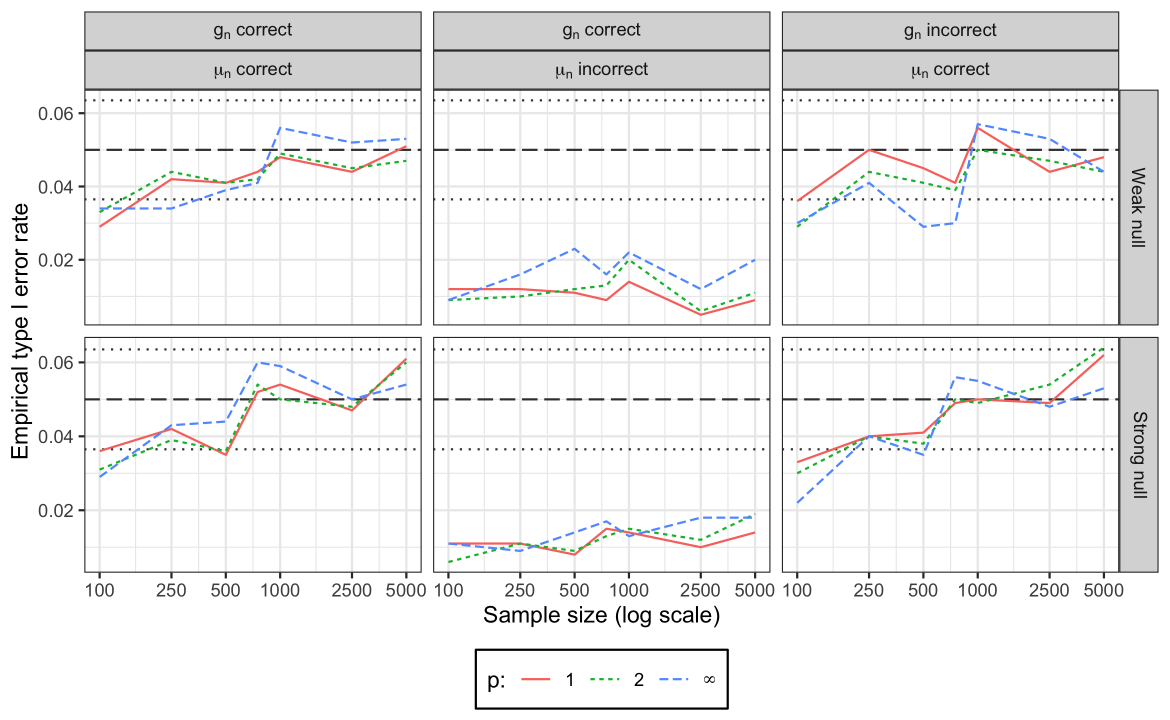
Refer to caption
Refer to caption
Figure 5: Empirical type I error rate (i.e. the fraction of tests with p<0.05p<0.05) of nominal α=0.05\alpha=0.05 level tests using the parametric nuisance estimators across the two types of null hypotheses and seven sample sizes. Panels in the top row were generated under the weak null where μ0\mu_{0} depends on aa, but θ0\theta_{0} does not. Panels in the bottom row were generated under the strong null where neither μ0\mu_{0} nor θ0\theta_{0} depends on aa. Columns indicate the type of nuisance estimators used. Horizontal wide-dash lines indicate the nominal 0.05 test size, and horizontal dotted lines indicate sampling error bounds were the true size 0.05. In the third and fourth columns from the left, the empirical sizes are off the scale of the figure, and in particular are larger than 0.5 in all cases.
Refer to caption
Figure 6: Empirical power (i.e. the fraction of tests with p<0.05p<0.05) of nominal α=0.05\alpha=0.05 level tests using the parametric nuisance estimators across the four types of alternative hypotheses and three sample sizes. Columns indicate the type of nuisance estimators used.

Figure 7 displays the empirical power of our tests in the second numerical study. We note that the number kk of levels of the exposure had little impact on the power of the tests for any sample or any under alternative hypothesis. In each case, the power increased with the sample size nn.

Refer to caption
Figure 7: Empirical power of nominal α=0.05\alpha=0.05 level tests in the second numerical study using our method with cross-fitted, correctly-specified parametric nuisance estimators. The xx-axis is the ratio of kk, the number of levels of the exposure, to nn, the sample size. Columns indicate the alternative hypothesis used to generate the data.

Additional results from analysis of the effect of BMI on immune response

Figure 8 shows the estimated primitive functions Ωn\Omega_{n} and 95% uniform confidence bands as a function of BMI for the analysis of CD4+ responses (left) and CD8+ responses (right).

Refer to caption
Figure 8: Estimated functions Ωn\Omega_{n} (solid line) and 95% uniform confidence band (dashed lines) for the analysis of CD4+ responses (left) and CD8+ responses (right) presented in the article.

References

  • Andrews (1997) Andrews, D. W. K. (1997). A Conditional Kolmogorov Test. Econometrica, 65(5):1097–1128.
  • Bang and Robins (2005) Bang, H. and Robins, J. M. (2005). Doubly robust estimation in missing data and causal inference models. Biometrics, 61(4):962–973.
  • Belloni et al. (2018) Belloni, A., Chernozhukov, V., Chetverikov, D., and Wei, Y. (2018). Uniformly valid post-regularization confidence regions for many functional parameters in Z-estimation framework. Ann. Statist., 46(6B):3643–3675.
  • Bickel et al. (1998) Bickel, P. J., Klaassen, C. A., Ritov, Y., and Wellner, J. A. (1998). Efficient and adaptive estimation for semiparametric models, volume 2. Springer New York.
  • Boudjellaba et al. (1992) Boudjellaba, H., Dufour, J.-M., and Roy, R. (1992). Testing causality between two vectors in multivariate autoregressive moving average models. Journal of the American Statistical Association, 87(420):1082–1090.
  • Cohen (1983) Cohen, J. (1983). The cost of dichotomization. Applied Psychological Measurement, 7(3):249–253.
  • Cox (1957) Cox, D. R. (1957). Note on grouping. Journal of the American Statistical Association, 52(280):543–547.
  • Díaz and van der Laan (2011) Díaz, I. and van der Laan, M. J. (2011). Super learner based conditional density estimation with application to marginal structural models. The International Journal of Biostatistics, 7(1):1–20.
  • Eubank and Spiegelman (1990) Eubank, R. L. and Spiegelman, C. H. (1990). Testing the goodness of fit of a linear model via nonparametric regression techniques. Journal of the American Statistical Association, 85(410):387–392.
  • Fedorov et al. (2009) Fedorov, V., Mannino, F., and Zhang, R. (2009). Consequences of dichotomization. Pharmaceutical Statistics, 8(1):50–61.
  • Gill and Robins (2001) Gill, R. D. and Robins, J. M. (2001). Causal inference for complex longitudinal data: The continuous case. The Annals of Statistics, 29(6):1785–1811.
  • Granger (1980) Granger, C. (1980). Testing for causality: A personal viewpoint. Journal of Economic Dynamics and Control, 2:329 – 352.
  • Granger and Lin (1995) Granger, C. W. J. and Lin, J.-L. (1995). Causality in the long run. Econometric Theory, 11(3):530–536.
  • Hirano and Imbens (2005) Hirano, K. and Imbens, G. W. (2005). The Propensity Score with Continuous Treatments, chapter 7, pages 73–84. John Wiley & Sons, Ltd.
  • Horowitz and Spokoiny (2001) Horowitz, J. L. and Spokoiny, V. G. (2001). An adaptive, rate-optimal test of a parametric mean-regression model against a nonparametric alternative. Econometrica, 69(3):599–631.
  • Horvitz and Thompson (1952) Horvitz, D. G. and Thompson, D. J. (1952). A Generalization of Sampling Without Replacement from a Finite Universe. Journal of the American Statistical Association, 47(260):663–685.
  • Imai and van Dyk (2004) Imai, K. and van Dyk, D. A. (2004). Causal inference with general treatment regimes. Journal of the American Statistical Association, 99(467):854–866.
  • Jin et al. (2015) Jin, X., Morgan, C., Yu, X., DeRosa, S., Tomaras, G. D., Montefiori, D. C., Kublin, J., Corey, L., Keefer, M. C., Network, N. H. V. T., et al. (2015). Multiple factors affect immunogenicity of dna plasmid hiv vaccines in human clinical trials. Vaccine, 33(20):2347–2353.
  • Kennedy (2019) Kennedy, E. H. (2019). Nonparametric Causal Effects Based on Incremental Propensity Score Interventions. Journal of the American Statistical Association, 114(526):645–656.
  • Kennedy et al. (2017) Kennedy, E. H., Ma, Z., McHugh, M. D., and Small, D. S. (2017). Non-parametric methods for doubly robust estimation of continuous treatment effects. Journal of the Royal Statistical Society: Series B (Statistical Methodology), 79(4):1229–1245.
  • Luedtke et al. (2019) Luedtke, A., Carone, M., and van der Laan, M. J. (2019). An omnibus non-parametric test of equality in distribution for unknown functions. Journal of the Royal Statistical Society: Series B (Statistical Methodology), 81(1):75–99.
  • Neugebauer and van der Laan (2005) Neugebauer, R. and van der Laan, M. (2005). Why prefer double robust estimators in causal inference? Journal of Statistical Planning and Inference, 129(1-2):405–426.
  • Neugebauer and van der Laan (2007) Neugebauer, R. and van der Laan, M. J. (2007). Nonparametric causal effects based on marginal structural models. Journal of Statistical Planning and Inference, 137(2):419–434.
  • Nishiyama et al. (2011) Nishiyama, Y., Hitomi, K., Kawasaki, Y., and Jeong, K. (2011). A consistent nonparametric test for nonlinear causality–specification in time series regression. Journal of Econometrics, 165(1):112 – 127. Moment Restriction-Based Econometric Methods.
  • R Core Team (2020) R Core Team (2020). R: A Language and Environment for Statistical Computing. R Foundation for Statistical Computing, Vienna, Austria.
  • Robins (1986) Robins, J. (1986). A new approach to causal inference in mortality studies with a sustained exposure period – application to control of the healthy worker survivor effect. Mathematical Modelling, 7(9):1393 – 1512.
  • Robins (2000) Robins, J. M. (2000). Marginal structural models versus structural nested models as tools for causal inference. In Halloran, M. E. and Berry, D., editors, Statistical Models in Epidemiology, the Environment, and Clinical Trials, pages 95–133, New York, NY. Springer New York.
  • Robins et al. (1994) Robins, J. M., Rotnitzky, A., and Zhao, L. P. (1994). Estimation of regression coefficients when some regressors are not always observed. Journal of the American Statistical Association, 89(427):846–866.
  • Rotnitzky et al. (1998) Rotnitzky, A., Robins, J. M., and Scharfstein, D. O. (1998). Semiparametric regression for repeated outcomes with nonignorable nonresponse. Journal of the American Statistical Association, 93(444):1321–1339.
  • Rubin and van der Laan (2006) Rubin, D. and van der Laan, M. J. (2006). Extending marginal structural models through local, penalized, and additive learning. Working Paper 212, Division of Biostatistics, University of California at Berkeley, Berkeley, California.
  • Rubin (1973) Rubin, D. B. (1973). Matching to Remove Bias in Observational Studies. Biometrics, 29(1):159–183.
  • Scharfstein et al. (1999) Scharfstein, D. O., Rotnitzky, A., and Robins, J. M. (1999). Adjusting for nonignorable drop-out using semiparametric nonresponse models. Journal of the American Statistical Association, 94(448):1096–1120.
  • van der Laan et al. (2018) van der Laan, M. J., Bibaut, A., and Luedtke, A. R. (2018). CV-TMLE for nonpathwise differentiable target parameters. In van der Laan, M. J. and Rose, S., editors, Targeted Learning in Data Science: Causal Inference for Complex Longitudinal Studies, pages 455–481. Springer.
  • van der Laan et al. (2007) van der Laan, M. J., Polley, E. C., and Hubbard, A. E. (2007). Super learner. Statistical Applications in Genetics and Molecular Biology, 6(1).
  • van der Laan and Robins (2003) van der Laan, M. J. and Robins, J. M. (2003). Unified methods for censored longitudinal data and causality. Springer Science & Business Media.
  • van der Laan and Rose (2011) van der Laan, M. J. and Rose, S. (2011). Targeted learning: causal inference for observational and experimental data. Springer-Verlag New York.
  • van der Vaart and van der Laan (2006) van der Vaart, A. W. and van der Laan, M. J. (2006). Estimating a survival distribution with current status data and high-dimensional covariates. The International Journal of Biostatistics, 2(1).
  • van der Vaart and Wellner (1996) van der Vaart, A. W. and Wellner, J. A. (1996). Weak Convergence and Empirical Processes. Springer.
  • Westling et al. (2020) Westling, T., Gilbert, P., and Carone, M. (2020). Causal isotonic regression. Journal of the Royal Statistical Society: Series B (Statistical Methodology), 82(3):719–747.
  • Young et al. (2019) Young, J. G., Logan, R. W., Robins, J. M., and Hernán, M. A. (2019). Inverse Probability Weighted Estimation of Risk Under Representative Interventions in Observational Studies. Journal of the American Statistical Association, 114(526):938–947.
  • Zhang et al. (2016) Zhang, Z., Zhou, J., Cao, W., and Zhang, J. (2016). Causal inference with a quantitative exposure. Statistical Methods in Medical Research, 25(1):315–335. PMID: 22729475.
  • Zheng and van der Laan (2011) Zheng, W. and van der Laan, M. J. (2011). Cross-validated targeted minimum loss based estimation. In van der Laan, M. and Rose, S., editors, Targeted learning: causal inference for observational and experimental data, chapter 27, pages 459–473. Springer-Verlag New York, New York.