A Tree Adjoining Grammar Representation for Models Of Stochastic Dynamical Systemsfootnoteinfofootnoteinfo2
Abstract
Model structure and complexity selection remains a challenging problem in system identification, especially for parametric non-linear models. Many Evolutionary Algorithm (EA) based methods have been proposed in the literature for estimating model structure and complexity. In most cases, the proposed methods are devised for estimating structure and complexity within a specified model class and hence these methods do not extend to other model structures without significant changes. In this paper, we propose a Tree Adjoining Grammar (TAG) for stochastic parametric models. TAGs can be used to generate models in an EA framework while imposing desirable structural constraints and incorporating prior knowledge. In this paper, we propose a TAG that can systematically generate models ranging from FIRs to polynomial NARMAX models. Furthermore, we demonstrate that TAGs can be easily extended to more general model classes, such as the non-linear Box-Jenkins model class, enabling the realization of flexible and automatic model structure and complexity selection via EA.
keywords
System identification, tree adjoining grammar, evolutionary algorithmsfootnoteinfo]This research is supported by the Dutch Organization for Scientific Research (NWO, domain TTW, grant: 13852) which is partly funded by the Ministry of Economic Affairs of The Netherlands. footnoteinfo2]Corresponding author D. Khandelwal.
, ,
1 Introduction
In recent years, there has been a resurgence in the use of Evolutionary Algorithms (EAs) for data-driven modelling of dynamical systems. Undoubtedly, one of the main driving forces for this is the steady growth of computation power. EAs are being increasingly used in a multitude of engineering domains and life science (Eiben et al. 2003; Arias-Montano et al. 2012). Across several domains, EAs have generated results that are competitive and, sometimes, even surprising (Eiben et al. 2003). Another factor contributing to the growing popularity of EAs is that these algorithms can be used to generate solutions for complex problems for which no systematic solution approach exists in general. In parametric system identification, the estimation of model structure and model complexity is one such problem.
Model structure selection is a classical problem in system identification. Over the years, a variety of methods for system identification have been developed. Each of these methods adopt different approaches to solve the problem of model structure selection. While methods like Prediction Error Minimization (PEM) treat model structure selection as a user’s choice (Ljung 1999), other methods (for example, Pillonetto et al. 2011, Laurain et al. 2020) rely on a flexible model structure, and attempt to estimate or control the complexity of the model-to-be-estimated via regularization. Furthermore, the appropriate model complexity is often chosen by ranking models based on an information metric, such as AIC, BIC, or based on a user-defined complexity measure (Rojas et al. 2014). In cases where the number of candidate models grows combinatorially with respect to the length (or the complexity) of the model, a ranking-based complexity selection strategy becomes intractable, restricting model structure selection to regularization or shrinkage based methods.
As a consequence of the aforementioned challenges, heuristics-based methods such as EAs have been used to estimate model structure and complexity, with a fair amount of success. However, the application of EAs have been, to some extent, superficial. The premise of the biologically-inspired heuristics used in EAs is that the solutions of a given problem can be constructed from fundamental building blocks, and these fundamental components can be interchanged between different solutions. In the system identification literature, the proposed EA-based approaches to model structure and complexity selection can be categorized as follows:
- i)
approaches that choose a fixed model structure and use EAs to determine the appropriate model complexity (or model terms), and
- ii)
approaches that use EAs to explore model structure and model complexity.
In the first category of EA-based approaches, the basic building blocks of an EA are chosen such that only models with a specific model structure can be generated. Hence, these approaches cannot be typically extended to other model structures without significant modifications. This approach can be found in Fonseca and Fleming 1996; Rodriguez-Vazquez et al. 2004; Rodríguez-Vázquez and Fleming 2000, where the authors use EAs to perform term selection within a chosen model structure. This approach is also used in Kristinsson and Dumont 1992, where the authors use GAs to estimate pole-zero locations for ARMAX models.
In the second category of EA-based approaches, more generic set of building blocks are used in the EA, allowing the generation of models with arbitrary model structures. In this case, EAs are used to determine not just the appropriate complexity of the model, but also the approprite model structure (e.g., in terms of the non-linear functions to be included in the model). However, unrestrained generation of arbitrary model structures using EA may result in models that are not well-posed, e.g., models with discontinuities, non-causality, or finite escape-time. Typically, these problems are avoided by using arbitrary ad-hoc solutions, e.g, setting all discontinuities to 0. Another common drawback of EA-based approaches that fall in the second category is that prior knowledge of the dynamical system cannot be incorporated systematically in the identification procedure. In Madár et al. 2005, the authors use GP to identify NARMAX models that may contain arbitrary non-linearities. While the authors are interested in models that are linear-in-the-parameters, GP may return models that do not belong to that class. Consequently, the authors use an ad-hoc solution to ensure that the candidate model structures generated by GP are linearly parameterized. A similar approach was used in Quade et al. 2016 with a larger set of mathematical operations. Again, the proposed approach does not allow for systematic inclusion of model structure constraints or prior knowledge of the system. A slightly different approach is used in Gray et al. 1998, where the authors use GP to construct linear or non-linear models from basic elements like SIMULINK blocks and static non-linearities. Again, the combination of various SIMULINK blocks cannot be systematically structured to avoid ill-posed models.
In this paper, we propose a generative grammar based representation of stochastic parametric dynamical systems. The proposed representation allows for the generation of complex, yet well-posed dynamical models by combining a set of fundamental building blocks in well-specified ways. The resulting generative declaration of models defines a notion of model set that is more generalized than that conventionally used, for example, in Ljung 1999. The generative grammar used in this work is called Tree Adjoining Grammar (TAG) (Joshi and Schabes 1997). The use of TAG in an EA-based approach makes it possible to develop a system identification framework where EAs are used to automatically determine the structure and complexity of a model from a generic, well-posed class of dynamical models, while systematically incorporating model structure constraints and prior knowledge. A preliminary concept of the proposed framework (without proofs) was presented in Khandelwal et al. 2019b. The proposed approach for grammar-based identification was found to produce results that were comparable to state-of-the-art non-linear system identification approaches, while using no specialized knowledge of the benchmark system being identified.
The main contributions of this paper are the following. We present a detailed discussion on the discrete-time input-output representation of dynamical systems using TAG, and introduce a new notion of a model set defined by the generative capacity of a TAG. Subsequently, we develop a TAG for the polynomial NARMAX model class. We prove that any model structure generated by the proposed TAG belongs to the class of polynomial NARMAX models, and conversely, any polynomial NARMAX model can be represented using the proposed TAG (for which an algorithm is also proposed). We demonstrate that the model set corresponding to the proposed TAG includes, as special cases, other commonly used model structures such as FIR, ARX and Truncated Volterra series models. We also demonstrate that the proposed representation can be easily extended to other model structures (namely polynomial Non-linear Box-Jenkins, or NBJ). Note that, while the TAG-based model set notion developed in this contribution is motivated by its applicability in an EA-based identification methodology, the identification approach itself is not in the scope of the present contribution. A preliminary version of such an identification methodology can be found in Khandelwal et al. 2019a and Khandelwal et al. 2019b.
The contributions in this paper differ from Khandelwal et al. 2019b in the following respects:
- •
we formulate a TAG for a larger class of dynamical systems (the polynomial NARMAX class), and prove their equivalence,
- •
we provide an algorithm to compute an equivalent TAG representation of a given polynomial NARMAX model,
- •
we illustrate, via examples, the restriction (and generalization) of the proposed TAG in order to generate models with more specific (or generic) structures.
The remainder of the paper is structured as follows. The concept of TAG is introduced, both informally and formally, in Sec. 2. In Sec. 3 we introduce the notion of model set as defined by a given TAG, and propose a TAG that generates the class of polynomial NARMAX models. Several examples are used to illustrate the concept in Sec. 4, followed by concluding statements in Sec. 5.
2 Tree Adjoining Grammar
To set the stage for the development of TAG for stochastic non-linear systems, first we introduce the basic concepts of TAG. Since TAG was initially developed from linguistic considerations, a linguistic example will be used to illustrate the methodology. This will be followed by formal definitions. To make the example illustrative, we first specify an example string, and then infer a TAG that would generate the given string. Conversely, for the formal definitions, we will begin with the basic components of a TAG and lead up to the definition of TAG and operations that can be performed on TAGs.
2.1 An informal description
Informally, a formal grammar can be described as a set of rules for generating strings. The resulting set of strings is called the language generated by the grammar. In contrast, TAG describes a set of rules for generating trees. The resulting set of trees is called the tree language of the TAG. The yield of all the trees in the tree set subsequently determines the corresponding language.
The following example has been derived from Joshi and Schabes 1997. Consider the sentence “A man saw Mary”. Simple grammatical constructs can be used to decompose the given sentence into its basic components. For example, the sentence consists of articles (“A”), nouns (“man”, “Mary”) and verbs (“saw”). Other underlining structures, such as subjects and predicates, can also be observed in the sentence. The sentence, together with the underlying grammatical structure can be represented in a single tree structure as shown in Fig. 1. The tree depicted in Fig. 1 is called a derived tree. The yield of a derived tree are the labels associated with the leaves of the tree. Hence, the yield of the derived tree in Fig. 1 is “A man saw Mary”.
The given derived tree can be obtained by combining basic building blocks that are constituents of the TAG. Fig. 2 depicts the set of initial trees and auxiliary trees , collectively known as elementary trees, that can be combined in specific ways to produce the derived tree in Fig. 1. The set of initial trees can be informally described as a set of non-recursive replacement rules that can be used to generate a set of trees. The set of auxiliary trees can be described as a set of recursive replacement rules. Consequently, each auxiliary tree has a terminal node with the same label as that of its root node.
The downward arrow symbol and the star symbol in Fig. 2 represent nodes in a tree that are available for a substitution and adjunction operation respectively. A substitution operation can be used to substitute an initial tree into, for instance, another initial tree, if and only if the latter has a terminal node (leaf) with a label that matches the label of the root node of the prior. On the other hand, adjunction can be loosely described as the operation of inserting an auxiliary tree into a syntactic tree. Adjunction of an auxiliary tree can take place on a non-terminal node of a syntactic tree if and only if the node has a label that matches the label of the root node of the auxiliary tree to be adjoined.
Consider the following sequence of operations. The initial tree can be substituted in at the location of the “sub” node. Let’s denote the resulting tree as . The tree is an example of a syntactic tree, a tree obtained by applying an arbitrary number of substitution and adjunction operations to a given initial tree. Again, the initial tree can be substituted to the syntactic tree at the location of the “pred” node. Let the result be denoted as . Note that has the same structure as the example in Fig. 1, upto the last level of the derived tree, where specific articles, nouns and verbs are substituted in the tree to obtain the yield “a man saw Mary”. Substitution can be performed on a initial tree or syntactic tree as long as there exist nodes available for substitution, marked by . A derived tree is a syntactic tree in which none of the terminal nodes (leaves) are available for substitution. The initial and auxiliary trees provide an alternative representation, the derivation tree, as shown in Fig. 3(a). Based on the TAG in Fig. 2, more complex sentences can also be generated. For example, the auxiliary tree can be adjoined to the root node of since both root nodes have the label “sentence”. This operation effectively adds an adverb before the sentence, yielding the sentence “yesterday a man saw Mary”. The resulting derivation tree is depicted in Fig. 3(b).
The set of all derived trees that can be obtained, by starting from a given start symbol, say “sentence”, and applying an arbitrary number of adjunctions and/or substitutions using elementary trees is called the tree language of the corresponding TAG. The string yield of all trees in the tree set is called the string language of the corresponding TAG.
We can now introduce the formal definitions of the concepts that were informally described in this example.
2.2 The formal definitions
The formal definitions of TAG and related concepts can be found in Joshi and Schabes 1997 and Kallmeyer 2009. These definitions are reproduced here for completeness.
Definition 1
A finite tree is a directed graph, denoted by , where, is the set of vertices, is the set of edges, and is the root node, such that
- -
contains no cycles,
- -
has in-degree (number of incoming edges) 0,
- -
All have in-degree 1,
- -
Every is accessible from ,
- -
A vertex with out-degree (i.e., number of outgoing edges) 0 is a leaf.
Definition 2
A labeling of a graph over a signature is a pair of functions and , with being a set of disjoint alphabets.
For the next definitions, assume and to be disjoint sets of non-terminals and terminals, respectively.
Definition 3
A syntactic tree is an ordered, labelled tree such that the label for each vertex with out-degree at least 1 and for each leaf .
Definition 4
An auxiliary tree is a syntactic tree such that there is a unique leaf , marked as foot node, with . An auxiliary tree is denoted as .
Definition 5
An initial tree is a non-auxiliary syntactic tree.
With the basic concepts defined, we can now define TAG, and the related operations.
Definition 6
A Tree Adjoining Grammar is a tuple , where
- -
are disjoint alphabets of non-terminals and terminals,
- -
is a start symbol,
- -
is a finite set of initial trees and is a finite set of auxiliary trees.
The set of trees is called elementary trees.

Definition 7 (Substitution)
Let be a syntactic tree and be an initial tree and . The result of substituting into at node , denoted as , is defined as follows
- -
If is not a leaf or is a foot node or , then is not defined,
- -
otherwise, with
(1) and
(2)
The substitution operation is illustrated in Fig. 4(a).
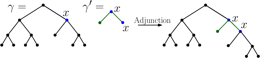
Definition 8 (Adjunction)
Let be a syntactic tree and be an auxiliary tree and with out-degree at least 1. The result of adjoining into at node , denoted as , is defined as follows
- -
if then is undefined,
- -
else with
(3) and
(4)
The adjunction operation is illustrated in Fig. 4(b).
Recall that a tree obtained by performing an arbitrary number of valid substitution and adjunction operations to an initial tree with is called a derived tree (for example, as in Fig. 1). Also recall that the substitution and adjunction operations performed can be represented in a tree representation called derivation tree (for example, as in Fig. 3). A derived tree is said to be saturated if all leaves of the derived tree belong to the set and cannot be further substituted. The corresponding derivation tree is also said to be saturated.
Definition 9 (Tree language and string language)
Let be a TAG. The tree language of grammar is defined as the set of all saturated derived trees in with root .
The string language of is the set of yields of the trees in .
3 TAG Description of Dynamical Systems
In this Section, we define a notion of model set based on TAG and propose a TAG for a generic class of dynamical models - the polynomial NARMAX class.
3.1 Model set
Consider the following discrete-time input-output representation of a non-linear dynamical model
| (5) |
where are the input and output signals at time-instant , is a noise signal independent of input , constants and are the corresponding maximum time-lags and the non-linear function belongs to an arbitrary set of functions . In PEM, the set of functions , also known as the model set, along with a specified choice for and , is determined by a user based on expert knowledge, prior information and informative experiments. It will be demonstrated in Sec. 3.2 that TAG can be used to generate trees that yield non-linear functions with desirable structural properties and varying choices of arguments (time lags of the involved and signals). This capability of TAG leads to a more generalized notion of model set . In order to formalize this concept, we introduce a function that maps from function to the right-hand-side expression in (5) (in string form). We can now define a new notion of model set, based on TAG, defined as follows.
Definition 10
For a given TAG , the corresponding model set is defined as the set of models in the form of (5) such that .
Note that this is a more generalized notion of model set as compared to that used in PEM. In PEM, a model set is typically determined by choosing a fixed model structure along with a suitable parameterization (i.e. model complexity). On the other hand, in this work, the choice of initial and auxiliary trees of a TAG automatically determines the model set. The advantage of such a declaration of a model set is that, when no prior information is available, the model set can be chosen to span a number of commonly used model classes without a prior specification of the model complexity. On the other hand, when prior information on the structure or complexity of the model is available, the grammar can be suitably refined to restrict the model set. In the subsequent sections, we propose a TAG for a generic model class, and demonstrate that the resulting model set spans a number of model structures commonly used in PEM.
3.2 The polynomial NARMAX model class
The NARMAX model class is a flexible class on non-linear input-output dynamical models, see Leontaritis and Billings 1985. The polynomial NARMAX model class is the set of all NARMAX models where the non-linear relationships are of the polynomial kind. Polynomial NARMAX is a convenient model representation since any continuous function on a closed space can be approximated arbitrary well using polynomial functions (based on Weierstrass’ theorem, see Stone 1948). Furthermore, the family of polynomial NARMAX models includes, as special cases, other commonly used model classes such as FIR and ARMAX. It will be shown that these models can be generated by suitably restricting the TAG presented here.
A discrete-time SISO polynomial NARMAX model can be represented as (see Billings 2013)
| (6) |
where is the order of the polynomial non-linearity, are the model parameters, and is a vector consisting of the past input, output and noise values building up the regressors
| (7) |
We will also use the following alternative and equivalent representation for polynomial NARMAX models:
| (8) |
where is the number of model terms, are the model parameters, are the exponents for output, input and noise terms.
3.3 Proposed TAG representation
In this section we propose a TAG for the polynomial NARMAX model class. The proposed TAG captures the structural relationships in (8). In the sequel, the time index will be dropped in the context of the proposed TAG, as will be used to denote a backward time shift. For convenience, introduce the following notation. For a given model in the form of (8), define , and . For the model term, the sequence of delays in the input, noise and output factors are denoted by , , respectively.
Theorem 1
PROOF.
For the first part of the proof, we show that for any polynomial NARMAX model in the form of (8), there exists a derivation tree such that the resulting derived tree has a yield that is equal to the RHS of (8). Algorithm 1 constructs such a derivation tree for a given polynomial NARMAX model. The procedure Delays adjoins auxiliary tree to the derivation tree at vertex . The algorithm constructs the derivation tree by introducing the first factor ( or ) of each of the model terms, and subsequently building each of the branches by introducing the remaining factors with the corresponding delays and exponents.
For the second part of the proof, it needs to be shown that all expressions in , i.e., yields of all possible trees generated by , are RHS expressions of polynomial NARMAX models. This is proven by structural induction. We first observe that the simplest tree in is the initial tree with the yield . This corresponds to the model
| (9) |
which belongs to the polynomial NARMAX class. Now, consider an arbitrary saturated derived tree whose yield is the RHS of a polynomial NARMAX model. This implies that the yield is a polynomial expression in terms of the factors , and . To complete the principle of induction, it must be shown that any possible adjunction to results in a new tree in whose yield is also a polynomial expression in terms of the aforementioned factors.
For convenience, the auxiliary trees are grouped based on the operators involved - are called additive-type auxiliary trees, are called multiplicative-type, and is called delay-type auxiliary tree. The following adjunctions be made on :
- •
adjunction of an additive-type tree. Such an adjuction introduces an input, output or noise term additively in the expression while respecting the causality of the expression. Hence the resulting expression is also a polynomial;
- •
adjunction of a multiplicative-type tree. This simply introduces multiplicative factors to an existing model term, and hence, the resulting expression is also a polynomial;
- •
adjunction of a delay-type tree. This operation simply adds delays to an existing monomial, and hence preserves the polynomial structure of the expression.
Since all possible operations yield a causal polynomial expression, it can be concluded that consists of only dynamical polynomial expressions in terms of the factors and which corresponds to a polynomial NARMAX model. This concludes the proof. ∎
Theorem 1 demonstrates that structural properties of a rich class of dynamical models can be captured within a compact set of trees of a TAG. The expansive representational capability of TAG can be exploited using EAs such as GP to identify models without prior specification of structure and complexity, as demonstrated in Khandelwal et al. 2019b. Furthermore, Algorithm 1 provides a method to compute the derivation tree representation of a given polynomial NARMAX model in terms of grammar . Consequently, available prior information about the model of the system can be translated to TAG representation (or incorporated in tree sets ), thereby making the evolutionary search more efficient. Hence, the use of TAG enables identification within a larger class of dynamical models without requiring user-interaction, while simultaneously allowing the user to restrict the evolutionary search effectively.
4 Illustrations
In this section we discuss aspects of TAG useful for EA-based SI. We demonstrate the use of TAG to generate polynomial NARMAX models. It is also shown that models belonging to simpler model classes can be generated by scaling down the set of elementary trees of appropriately. Furthermore, more flexible model classes can be represented by scaling up the set of elementary trees. This is demonstrated by extending the proposed TAG to generate Non-linear Box Jenkins (NBJ) models.
4.1 Model generation using
Three illustrative examples are used to demonstrate the generation of models using . The models generated belong to the ARX, polynomial NARX and polynomial NARMAX model classes. It will be demonstrated that by restricting the elementary trees and to subsets of the elementary trees in the proposed TAG , we can generate models that only belong to model sub-classes that are properly included in the set of polynomial NARMAX models, such as FIR and truncated Volterra series.
4.1.1 ARX example
ARX models can be described by the equation
| (10) |
where are coefficients. The grammar can be used to generate ARX models by restricting the auxiliary tree set as
| (11) |
Consider the example depicted in Fig. 7(a). Tree (A) is a derivation tree with initial tree at the root node, and auxiliary trees and in subsequent vertices. The edges are labelled with Gorn addresses of vertices in the auxilliary trees at which adjunctions take place. Performing the adjunctions results in derived tree (B) in Fig. 7(a). The RHS of the resulting model appears at the leaves of the derived tree, and the corresponding model is
| (12) |
4.1.2 NARX example
Polynomial NARX models can be described by the equation
| (13) |
By restricting auxiliary trees to the set
| (14) |
we can restrict the proposed grammar to generate polynomial NARX models only. Consider the example derivation tree (A) in Fig. 7(b), which is an extension of the previous example. The derivation tree consists of the initial tree , and auxiliary trees and . Performing the adjunctions described by the derivation tree results in the derived tree (B) in Fig. 7(b). The corresponding symbolic model is
| (15) |
4.1.3 NARMAX example
This example builds on the previous example by using the complete auxiliary tree set and adjoining trees and to the tree . The new derivation tree and derived tree are depicted in Fig. 7(c). The corresponding model,
| (16) |
is a polynomial NARMAX model.
4.2 Non-linear Box-Jenkins Extension
Just like the proposed grammar can be scaled down to generate specific dynamic sub-classes, it can also be extended to generate models that belong to a more generalized class of models. We illustrate this by extending the proposed grammar to a more generalized models structure - Non-linear Box Jenkins (NBJ).
In the case of linear systems, a Box-Jenkins model structure is an extension of the Output Error (OE) model structure, where the error is modelled as an ARMA process (Ljung 1999). The BJ class also includes, as special cases, other linear model structures such as ARMAX and OE. In the same spirit, NBJ model structure can be expressed as a Non-linear Output Error (NOE) model where the error is subsequently modelled as a NARMA process. The NBJ model structure is given by the following equations
| (17) |
where and are polynomial functions in terms of their arguments. Notice that the RHS expressions of the equations describing the process and noise dynamics have the same structure that was studied in Sec. 3.2 for NARMAX models (see (8)). Hence, the proposed TAG can be extended to generate NBJ models. Fig. 8 depicts the initial and auxiliary trees of the grammar for NBJ model structures . The structure of the initial tree ensures that all elements in contain two expressions, separated by a comma, that represent the functions and respectively. Each of these expressions can be expanded by adjoining auxiliary trees that ensure that the polynomial structure is maintained.
5 Conclusions
We presented a TAG based concept of a model set, that is more general than that commonly used in the system identification literature. A TAG was proposed that captures the dynamical structure of polynomial NARMAX models. It was demonstrated that sub-classes of the polynomial NARMAX class can be represented by choosing an appropriate subset of the elementary trees of . Similarly, more flexible model classes like Non-linear Box-Jenkins can be represented by extending the set of elementary trees. This illustrates that a compact set of elementary trees can be used to express the dynamical relationships across a variety of model classes, thereby enabling the design of TAG-based EA approaches for SI that require minimal user-interaction. The practical soundness of this concept has been demonstrated in Khandelwal et al. 2019b, where a TAG-based EA approach was used to identify a non-linear benchmark dataset with minimal user-interaction, and also in Khandelwal et al. 2019a, where the same TAG-based EA approach is used to identify multiple real physical systems and benchmark data set with minimal changes in the methodology itself.
References
- Arias-Montano et al. (2012) Arias-Montano, A., Coello, C. A. C., and Mezura-Montes, E. (2012). Multiobjective evolutionary algorithms in aeronautical and aerospace engineering. IEEE Transactions on Evolutionary Computation, 16(5):662–694.
- Billings (2013) Billings, S. A. (2013). Nonlinear system identification: NARMAX methods in the time, frequency, and spatio-temporal domains. John Wiley & Sons.
- Eiben et al. (2003) Eiben, A. E., Smith, J. E., et al. (2003). Introduction to evolutionary computing, volume 53. Springer.
- Fonseca and Fleming (1996) Fonseca, C. M. and Fleming, P. J. (1996). Non-linear system identification with multiobjective genetic algorithms. In Proc. of IFAC World Congress, pages 1169–1174, San Francisco, USA.
- Gorn (1965) Gorn, S. (1965). Explicit definitions and linguistic dominoes.
- Gray et al. (1998) Gray, G. J., Murray-Smith, D. J., Li, Y., Sharman, K. C., and Weinbrenner, T. (1998). Nonlinear model structure identification using genetic programming. Control Engineering Practice, 6(11):1341–1352.
- Joshi and Schabes (1997) Joshi, A. K. and Schabes, Y. (1997). Tree-adjoining grammars. In Handbook of formal languages, pages 69–123. Springer.
- Kallmeyer (2009) Kallmeyer, L. (2009). A declarative characterization of different types of multicomponent tree adjoining grammars. Research on Language and Computation, 7(1):55–99.
- Khandelwal et al. (2019a) Khandelwal, D., Schoukens, M., and Tóth, R. (2019a). Data-driven modelling of dynamical systems using tree adjoining grammar and genetic programming. In Proc. of the IEEE Congress on Evolutionary Computation, pages 2673–2680, Wellington, New Zealand.
- Khandelwal et al. (2019b) Khandelwal, D., Schoukens, M., and Tóth, R. (2019b). Grammar-based representation and identification of dynamical systems. In Proc. of the 18th European Control Conference (ECC), pages 1318–1323, Naples, Italy.
- Kristinsson and Dumont (1992) Kristinsson, K. and Dumont, G. A. (1992). System identification and control using genetic algorithms. IEEE Transactions on Systems, Man, and Cybernetics, 22(5):1033–1046.
- Laurain et al. (2020) Laurain, V., Tóth, R., Piga, D., and Darwish, M. A. H. (2020). Sparse rkhs estimation via globally convex optimization and its application in lpv-io identification. Automatica, 115:108914.
- Leontaritis and Billings (1985) Leontaritis, I. and Billings, S. A. (1985). Input-output parametric models for non-linear systems part i: deterministic non-linear systems. International journal of control, 41(2):303–328.
- Ljung (1999) Ljung, L., editor (1999). System Identification (2 Ed.): Theory for the User. Prentice Hall PTR.
- Madár et al. (2005) Madár, J., Abonyi, J., and Szeifert, F. (2005). Genetic programming for the identification of nonlinear input- output models. Industrial & engineering chemistry research, 44(9):3178–3186.
- Pillonetto et al. (2011) Pillonetto, G., Chiuso, A., and De Nicolao, G. (2011). Prediction error identification of linear systems: a nonparametric gaussian regression approach. Automatica, 47(2):291–305.
- Quade et al. (2016) Quade, M., Abel, M., Shafi, K., Niven, R. K., and Noack, B. R. (2016). Prediction of dynamical systems by symbolic regression. Physical Review E, 94(1):012214.
- Rodríguez-Vázquez and Fleming (2000) Rodríguez-Vázquez, K. and Fleming, P. J. (2000). Use of genetic programming in the identification of rational model structures. In Proc. of the European Conference on Genetic Programming, pages 181–192, Berlin, Heidelberg.
- Rodriguez-Vazquez et al. (2004) Rodriguez-Vazquez, K., Fonseca, C. M., and Fleming, P. J. (2004). Identifying the structure of nonlinear dynamic systems using multiobjective genetic programming. IEEE Transactions on Systems, Man, and Cybernetics-Part A: Systems and Humans, 34(4):531–545.
- Rojas et al. (2014) Rojas, C. R., Tóth, R., and Hjalmarsson, H. (2014). Sparse estimation of polynomial and rational dynamical models. IEEE Trans. Automat. Contr., 59(11):2962–2977.
- Stone (1948) Stone, M. H. (1948). The generalized weierstrass approximation theorem. Mathematics Magazine, 21(5):237–254.